Sufficient dimension reduction based on an ensemble of minimum average variance estimators

Abstract

We introduce a class of dimension reduction estimators based on an ensemble of the minimum average variance estimates of functions that characterize the central subspace, such as the characteristic functions, the Box–Cox transformations and wavelet basis. The ensemble estimators exhaustively estimate the central subspace without imposing restrictive conditions on the predictors, and have the same convergence rate as the minimum average variance estimates. They are flexible and easy to implement, and allow repeated use of the available sample, which enhances accuracy. They are applicable to both univariate and multivariate responses in a unified form. We establish the consistency and convergence rate of these estimators, and the consistency of a cross validation criterion for order determination. We compare the ensemble estimators with other estimators in a wide variety of models, and establish their competent performance.

and

t1Supported in part by NSF Grant DMS-08-06120.

t2Supported in part by NSF Grants DMS-07-04621 and DMS-08-06058.

1 Introduction

Sufficient dimension reduction [Li (1991, 1992), Cook and Weisberg (1991), Cook (1994, 1996)] is a methodology for reducing the dimension of predictors while preserving its regression relation with a response. The reduction is achieved by projecting the raw predictors on to a lower-dimensional subspace. Let $(X,Y)$ be a pair of random vectors of dimensions $p$ and $s$. In this section we tentatively assume $s=1$. Let ${\mathcal{S}}$ denote a subspace of $\mathbb{R}^{p}$, and let $P_{\mathcal{S}}$ denote the orthogonal projection on to ${\mathcal{S}}$. If $Y$ and $X$ are independent conditioning on $P_{\mathcal{S}}X$, then $P_{\mathcal{S}}X$ can be used as the predictor without loss of regression information. Such subspaces ${\mathcal{S}}$ are called dimension reduction subspaces. The intersection of all such subspaces ${\mathcal{S}}$, if itself satisfies the conditional independence, is called the central subspace [Cook (1994)], and is denoted by ${\mathcal{S}}_{Y|X}$. Under mild conditions [Cook (1996), Yin, Li and Cook (2008)], the central subspace is well defined and is unique.

A closely related concept is the notion of central mean subspace [Cook and Li (2002)], which is the intersection of all subspaces such that $E(Y|X)=E(Y|P_{\mathcal{S}}X)$. This subspace is written as ${\mathcal{S}}_{E(Y|X)}$. Evidently, if conditional distribution of $Y$ given $X$ depends on $X$ only through $E(Y|X)$, then ${\mathcal{S}}_{Y|X}={\mathcal{S}}_{E(Y|X)}$. However, if this conditional distribution also depends on other functions of $X$, such as $\operatorname{var}(Y|X)$, then ${\mathcal{S}}_{E(Y|X)}$ is a proper subspace of ${\mathcal{S}}_{Y|X}$. Cook and Li (2002) noted that several previously introduced dimension reduction methods, such as the ordinary least squares [Li and Duan (1989), Duan and Li (1991)] and principal Hessian directions [Li (1992), Cook (1998)], actually estimates the central mean subspaces; whereas some other pre-existing estimates, such as the sliced inverse regression (SIR), the SIR-II [Li (1991)] and the sliced average variance estimator (SAVE) [Cook and Weisberg (1991)], can recover additional directions in the central subspace.

Yin and Cook (2002) extended central mean subspace to central moment subspace, based on the relation $E(Y^{k}|X)=E(Y^{k}|P_{\mathcal{S}}X)$, which is written as ${\mathcal{S}}_{E(Y^{k}|X)}$. This provides us with a graduation between the central mean subspace and the central subspace. That is, for sufficiently large $k$, the subspace spanned by $\{{\mathcal{S}}_{E(Y^{\ell}|X)}$, $\ell=1,\ldots,k\}$ approaches the central subspace. Zhu and Zeng (2006) showed that the central mean subspaces for $E(e^{\iota tY}|X),t\in\mathbb{R}$, when put together, recovers the central subspace, and exploited this relation to develop a Fourier transformation method to estimate the central subspace. Here and throughout, we use $\iota$ to denote the imaginary unit $\sqrt{-1}$. More recently, Zeng and Zhu (2010) developed a general integral transform method. Both papers hint at the following fact: if one can estimate the central mean subspace of $E[f(X)|Y]$ for sufficiently many functions $f$, then one can recover the central subspace.

In a seminal paper, Xia et al. (2002) introduced a dimension reduction method, called the minimum average variance estimator (MAVE), based on estimation of the gradient of the conditional expectation $E(Y|X)$. This method has three main advantages: (1) it estimates the central mean subspaces exhaustively; (2) it does not impose strong assumptions on the distribution of $X$; (3) its computation can be broken down into iterations between two quadratic optimization steps, each of which having an explicit solution. However, a drawback of this method is that it cannot estimate directions outside the central mean subspace. For example, it cannot recover directions in the conditional variance function $\operatorname{var}(Y|X)$. To remedy this deficiency, Xia (2007) and Wang and Xia (2008), respectively, proposed density MAVE (DMAVE) and sliced regression (SR) that can exhaustively estimate the central subspace. The former is based the estimation of the gradients of the functions $E\{H[(Y-a)/b]|X\}$, where $H$ is a known probability density function, $a\in(-\infty,\infty)$ and $b\in(0,\infty)$. The latter is based on the estimation of the gradients of the functions $E[I(Y\leq c)|X]$, where $c$ is an arbitrary constant. Here, again, we see the echo of the same basic fact that estimating the central mean subspaces for a rich enough family of functions is equivalent to estimating the central subspace itself.

The ensemble approach introduced in this paper is based on the same fact, but it is more general, more flexible and, in the numerical examples we considered, more efficient. In broad outlines the procedure can be described as follows. Consider a general family $\mathfrak{F}$ of functions of $Y$. For each $f\in\mathfrak{F}$, let ${\mathcal{S}}_{E[f(Y)|X]}$ denote the central mean subspace for the conditional mean $E[f(Y)|X]$. We say that $\mathfrak{F}$ characterizes the central subspace if the subspace spanned by the collection of subspaces $\{{\mathcal{S}}_{E[f(Y)|X]}\dvtx f\in\mathfrak{F}\}$ is equal to the central subspace. We introduce a probability measure on $\mathfrak{F}$, and randomly sample functions $f_{1},\ldots,f_{m}$ from $\mathfrak{F}$ according to this probability. We then assemble the central mean subspaces ${\mathcal{S}}_{E[f_{\ell}(Y)|X]}$, $\ell=1,\ldots,m$, together to recover the central subspace.

In principle, the ensemble approach can be used in conjunction with any estimators of the central mean subspace to recover the central subspace, such as the ordinary least squares, the principal Hessian directions, MAVE and its two variants: the outer product of gradients (OPG) and the refined MAVE (RMAVE). In this paper we focus on its combination with MAVE and its variants, and refer to this combination the MAVE (OPG or RMAVE) ensemble. We show that these ensemble estimators exhaustively estimate the central subspace and that the RMAVE ensemble has the same convergence rate as RMAVE itself. We also introduce a cross validation criterion to determine the dimension of the central subspace, and establish its consistency. Through a number of simulation experiments, most of which are based on published models, we demonstrate the superb performance of the RMAVE ensemble based on the family $\mathfrak{F}=\{e^{\iota tY}\dvtx t\in\mathbb{R}\}$. We also explore other characterizing families, such as the Box–Cox transformations and wavelet basis.

The rest of the paper is organized as follows. In Section 2 we investigate what types of family $\mathfrak{F}$ can characterize the central subspace. We introduce the MAVE ensemble in Section 3 and outline the parallel developments for OPG ensemble and the RMAVE ensemble in Section 4. In Section 5 we introduce a cross validation criterion for order determination and discuss the choices of the characterizing family $\mathfrak{F}$, with emphasis on the characteristic function and the Box–Cox transformations. In Section 6 we establish the consistency and derive the convergence rate of the RMAVE ensemble, and establish the consistency of the cross validation estimator. In Section 7 we conduct simulation comparisons between the RMAVE ensemble and other estimators in a large variety of models. Some concluding remarks are made in Section 8.

2 Characterizing the central subspace

The basic fact that underlies our approach is that the dimension reduction subspaces for the conditional means $E[f(Y)|X]$, when combined in unison, can recover the dimension reduction subspace for $Y$ versus $X$. For this idea to work, the family of $f$ needs to be sufficiently rich, and in this section we rigorously pose and study this characterization problem.

Let $X$ be a $p$-dimensional random vector defined on $\Omega_{X}$ and $Y$ be an $s$-dimensional random vector defined on $\Omega_{Y}$. Let $\mathfrak{F}$ be a family of functions $f\dvtx\Omega_{Y}\to{\mathbb{F}}$, where $\mathbb{F}$ can be the set of real numbers $\mathbb{R}$ or complex numbers $\mathbb{C}$. Let ${\mathcal{S}}_{E[f(Y)|X]}$ denote the central mean subspace for the conditional mean $E[f(Y)|X]$, as defined in Cook and Li (2002) and Yin and Cook (2002). That is, ${\mathcal{S}}_{E[f(Y)|X]}$ is the intersection of all subspaces of $\mathbb{R}^{p}$ such that

$$E[f(Y)|X]=E[f(Y)|P_{\mathcal{S}}X].$$ (1)

Let ${\mathcal{S}}_{Y|X}$ denote the central subspace of $Y$ versus $X$ as defined in Cook (1994). That is, ${\mathcal{S}}_{Y|X}$ is the intersection of all linear subspaces of $\mathbb{R}^{p}$ such that

$$Y\perp\!\!\!\!\perp X|P_{\mathcal{S}}X.$$ (2)

Note that here we do allow $Y$ to be a random vector; whereas the mentioned previous works assume $Y$ to be a scalar. This relaxation is made possible by the transformation $f$, which takes value in the scalar field $\mathbb{F}$.

Definition 2.1.

Let $\mathfrak{F}$ be a family of measurable $\mathbb{F}$-valued functions defined on $\Omega_{Y}$. If

$$\operatorname{span}\bigl{\{}{\mathcal{S}}_{E[f(Y)|X]}\dvtx f\in\mathfrak{F}\bigr{\}}={\mathcal{S}}_{Y|X},$$ (3)

then we say the family $\mathfrak{F}$ characterizes the central subspace.

Let $F_{Y}$ denote the distribution of $Y$, and let $L_{2}(F_{Y})$ be the class of functions $f(Y)$ with finite variances, together with the inner product $\langle f_{1},f_{2}\rangle=E[f_{1}(Y)f_{2}(Y)]$. Let $L_{1}(F_{Y})$ be the class of functions $f(Y)$ such that$E|f(Y)|<\infty$, together with the norm $E|f(Y)|$. We denote the subspace on the left-hand side of (3) by ${\mathcal{S}}(\mathfrak{F})$. Note that $E[f(Y)|X]$ is finite if $f\in L_{1}(F_{Y})$.

Lemma 2.1

Suppose that $\mathfrak{F}\subseteq L_{1}(F_{Y})$. Then the following assertions hold: [(2)]

${\mathcal{S}}(\mathfrak{F})\subseteq{\mathcal{S}}_{Y|X}$.

If (1) being satisfied for all $f\in\mathfrak{F}$ implies (2), then ${\mathcal{S}}_{Y|X}\subseteq{\mathcal{S}}(\mathfrak{F})$.

Before proving this lemma we first note the following fact. If ${\mathcal{S}}$, ${\mathcal{S}}_{1}$ and ${\mathcal{S}}_{2}$ are linear subspaces of $\mathbb{R}^{p}$, then

$${\mathcal{S}}_{1}\subseteq{\mathcal{S}}_{2}\quad\mbox{if and only if}\quad\{{\mathcal{S}}\dvtx\mbox{${\mathcal{S}}$ contains ${\mathcal{S}}_{2}$}\}\subseteq\{{\mathcal{S}}\dvtx\mbox{${\mathcal{S}}$ contains ${\mathcal{S}}_{1}$}\}.$$ (4)

This can be easily seen by taking intersection on both sides of the equality. Proof of Lemma 2.1 (1) Let ${\mathcal{S}}$ be a subspace of $\mathbb{R}^{p}$ that contains ${\mathcal{S}}_{Y|X}$. Then (2) holds, and consequently (1) holds for all $f\in\mathfrak{F}$. This implies that ${\mathcal{S}}$ contains ${\mathcal{S}}_{E[f(Y)|X]}$ for all $f\in\mathfrak{F}$. Since ${\mathcal{S}}$ is a linear subspace, it must contain ${\mathcal{S}}(\mathfrak{F})$. Hence

$$\{{\mathcal{S}}\dvtx{\mathcal{S}}\mbox{ contains }{\mathcal{S}}_{Y|X}\}\subseteq\{{\mathcal{S}}\dvtx{\mathcal{S}}\mbox{ contains }{\mathcal{S}}(\mathfrak{F})\},$$

which, by (4), proves part 1.

(2) Let ${\mathcal{S}}$ be a subspace of $\mathbb{R}^{p}$ that contains ${\mathcal{S}}(\mathfrak{F})$. Then (1) holds for all $f\in\mathfrak{F}$. By assumption this implies (2), and consequently ${\mathcal{S}}$ contains ${\mathcal{S}}_{Y|X}$. Hence

$$\{{\mathcal{S}}\dvtx{\mathcal{S}}\mbox{ contains }{\mathcal{S}}(\mathfrak{F})\}\subseteq\{{\mathcal{S}}\dvtx{\mathcal{S}}\mbox{ contains }{\mathcal{S}}_{Y|X}\},$$

which, by (4), implies ${\mathcal{S}}_{Y|X}\subseteq{\mathcal{S}}(\mathfrak{F})$.

Let $\mathfrak{B}$ be the family of measurable indicator functions of $Y$. That is, $\mathfrak{B}=\{I_{B}\dvtx B\mbox{ is a Borel set in }\Omega_{Y}\}$. Note that $\mathfrak{B}\subseteq L_{2}(F_{Y})$.

Theorem 2.1.

If $\mathfrak{F}$ is a subset of $L_{2}(F_{Y})$ that is dense in $\mathfrak{B}$, then ${\mathfrak{F}}$ characterizes the central subspace.

Because $\mathfrak{F}$ is a subset of $L_{2}(F_{Y})$, it is also a subset of $L_{1}(F_{Y})$. Hence, by Lemma 2.1, it suffices to show that (1) being satisfied for all $f\in{\mathfrak{F}}$ implies (2).

Let ${\mathcal{S}}$ be a subspace such that (1) holds for all $f\in{\mathfrak{F}}$, and let $B$ be a Borel set in $\Omega_{Y}$. Because $\mathfrak{F}$ is dense in $\mathfrak{B}$ there is a sequence $\{f_{k}\}\subseteq{\mathfrak{F}}$ such that $\lim_{k\to\infty}E[I_{B}(Y)-f_{k}(Y)]^{2}=0.$ For any $g\in L_{2}(F_{X})$ we have

$$E\{g(X)[I_{B}(Y)-E(I_{B}(Y)|P_{\mathcal{S}}X)]\}$$

$$\qquad=E\{g(X)[I_{B}(Y)-E(f_{k}(Y)|P_{\mathcal{S}}X)]\}$$ (5)

$$\qquad\quad{}+E\{g(X)E[f_{k}(Y)-I_{B}(Y)|P_{\mathcal{S}}X]\}.$$

The square of the second term on the right is no more than

$$E[g^{2}(X)]E\{E^{2}[f_{k}(Y)-I_{B}(Y)|P_{\mathcal{S}}X]\}\leq E[g^{2}(X)]E\{E[f_{k}(Y)-I_{B}(Y)]^{2}\}\to 0.$$

Since $f_{k}\in{\mathfrak{F}}$ we have $E[f_{k}(Y)|P_{\mathcal{S}}X]=E[f_{k}(Y)|X]$. Hence the first term on the right-hand side of (2) can be rewritten as

$$E\{g(X)[I_{B}(Y)-E(I_{B}(Y)|X)]\}+E\{g(X)E[I_{B}(Y)-f_{k}(Y)|X]\}.$$ (6)

The first term is 0 by the definition of conditional expectation. The square of the second term in (6) is no more than

$$E[g^{2}(X)]E\{E^{2}[I_{B}(Y)-f_{k}(Y)|X]\}\leq E[g^{2}(X)]E\{[I_{B}(Y)-f_{k}(Y)]^{2}\}\to 0.$$

Since the left-hand side of (2) does not depend on $k$, and the right-hand side converges to $0$ as $k\to\infty$, we have $E\{g(X)[I_{B}(Y)-E(I_{B}(Y)|P_{\mathcal{S}}X)]\}=0.$ By the definition of conditional expectation the above being true for all $g\in L_{2}(F_{X})$ implies $E[I_{B}(Y)|P_{\mathcal{S}}X)]=E[I_{B}(Y)|X]$ almost surely. Since $B$ is an arbitrary Borel set in $\Omega_{X}$, this implies $Y\perp\!\!\!\!\perp X|P_{\mathcal{S}}X$.

This theorem synthesizes several recently developed methods in the literature, and also anticipates useful new ways to combine central mean subspaces into the central subspace. The following examples demonstrate its potential.

Example 2.1 ((Polynomials)).

Let $\mathfrak{F}\,{=}\,\{Y^{t}\dvtx t\,{=}\,1,2,\ldots\}$. Then ${\mathcal{S}}_{E[f(Y)|X]}\,{=}\break{\mathcal{S}}_{E(Y^{t}|X)}$. This is the type of dimension reduction subspaces studied by Cook and Li (2002), Yin and Cook (2002) and more recently Zhu and Zhu (2009). If the conditional moment generating function $E(e^{tY}|X)$ is finite in an open interval that contains 0, then $\mathfrak{F}$ is dense in $L_{2}(F_{Y})$, and hence characterizes ${\mathcal{S}}_{Y|X}$.

Example 2.2 ((Kernel density)).

Let $b>0$ and $H$ be a symmetric probability density function defined on $\mathbb{R}$. Let $\mathfrak{F}=\operatorname{span}\{b^{-1}H[(y-t)/b]\dvtx t\in\mathbb{R},b\in\mathbb{R}^{+}\}.$ Xia (2007) proposed a DMAVE method that, in effect, recovers ${\mathcal{S}}_{Y|X}$ by estimating ${\mathcal{S}}_{E[f(Y)|X]}$ for $f\in\mathfrak{F}$. This family is dense in $L_{2}(F_{Y})$ when $H$ is the normal density. See, for example, Fukumizu, Bach and Jordan (2009).

Example 2.3 ((Slices)).

Let $\mathfrak{F}=\{I_{(-\infty,t)}(y)\dvtx t\in\mathbb{R}\}$. Then $\mathfrak{F}$ is clearly dense in $\mathfrak{B}$. The method proposed by Wang and Xia (2008) is based on the estimation of ${\mathcal{S}}_{E[f(Y)|X]}$ for $f$ in this family.

Example 2.4 ((Box–Cox transformations)).

Let $Y$ be a nonnegative random variable, and consider the family of transformations

$$f_{t}(y)=\cases{\dfrac{y^{t}-1}{t},&\quad$t\neq 0$,\vspace*{2pt}\cr\log(y),&\quad$t=0$.}$$ (7)

This is the Box–Cox transformation [Box and Cox (1964)]. This family characterizes the central subspace because it contains the family in Example 2.1.

Example 2.5 ((Characteristic function)).

Let $\mathfrak{F}=\{e^{\iota ty}\dvtx t\in\mathbb{R}\}$, where $\iota=\sqrt{-1}$. Note that $E(e^{\iota tY}|X)$ is simply the conditional characteristic function of $Y|X$. It is well known that this family is dense in $L_{2}(F_{Y})$. It is used by Zhu and Zeng (2006) to recover the central mean subspace and central subspace, respectively, based on the assumption that $X$ is multivariate normal. This family is also our focus when we implement the ensemble estimators.

Example 2.6 ((Haar wavelets)).

Let

$$\psi(t)=\cases{1,&\quad$t\in[0,1/2)$,\cr-1,&\quad$t\in[1/2,1)$,\cr 0,&\quad otherwise.}$$

Consider the family $\mathfrak{F}=\{1\}\cup\{\psi(2^{n}y-k)\dvtx k=0,\ldots,2^{n}-1;n=1,2,\ldots\},$ where the 1 in $\{1\}$ represents the function of $y$ that always takes the value 1. This is the famous Haar basis often used in wavelet estimators. See, for example, Donoho and Johnstone (1994) and Antoniadis and Fan (2001). The Haar basis is obviously dense in $\mathfrak{B}$ and hence characterizes the central subspace.

In this paper we only consider parametric characterizing families $\mathfrak{F}$. That is, $\mathfrak{F}$ is of the form $\{f_{t}\dvtx t\in\Omega_{T}\}$ where $\Omega_{T}$ is a subset of a Euclidean space $\mathbb{R}^{q}$. All the characterizing families in the above examples are parametric. In the following, for a sequence of subspaces $\{{\mathcal{S}}_{k}\}$ and a subspace ${\mathcal{S}}$, we say $\lim_{k\to\infty}{\mathcal{S}}_{k}={\mathcal{S}}$ if ${\lim_{k\to\infty}}\|P_{{\mathcal{S}}_{k}}-P_{\mathcal{S}}\|=0$, where $\|\cdot\|$ is a matrix norm, such as the operator norm or the Frobenius matrix norm. The two norms are topologically equivalent, and makes no difference in asymptotic analysis. See, for example, Li, Zha and Chiaromonte (2005). Note that we are interested in ${\mathcal{S}}_{Y|X}$ via $\operatorname{span}\{{\mathcal{S}}_{E[f_{t}(Y)|X]}\dvtx t\in\Omega_{T}\}$, then a question arises is whether we can recover ${\mathcal{S}}_{Y|X}$ from a finite $t\in\Omega_{T}$. Indeed, we can. Theorem 2.2 below demonstrates that, with probability 1, the central subspace can be characterized by a finite number of functions in a characterizing family. In essence, it relies on the following fact: if a sequence of subspaces ${\mathcal{S}}_{m}$ converges to another subspace ${\mathcal{S}}$ from within, then the norm $\|{\mathcal{S}}_{m}-{\mathcal{S}}\|$ is discrete in nature; that is, if this norm converges to 0 then it must be identically 0 for large $m$. This phenomenon is also noticed in Yin, Li and Cook (2008). The next lemma, albeit simple, reveals this discrete nature of dimension reduction.

Lemma 2.2

Let ${\mathcal{S}}_{1}\subseteq{\mathcal{S}}_{2}$ be two subspaces of $\mathbb{R}^{p}$. Then $\|P_{{\mathcal{S}}_{2}}-P_{{\mathcal{S}}_{1}}\|$ is either 0 or no less than 1.

If ${\mathcal{S}}_{1}={\mathcal{S}}_{2}$, then $\|P_{{\mathcal{S}}_{2}}-P_{{\mathcal{S}}_{1}}\|=0$. If ${\mathcal{S}}_{1}\neq{\mathcal{S}}_{2}$, then direct difference ${\mathcal{S}}_{2}\ominus{\mathcal{S}}_{1}$ is nonempty. We know that in this case $P_{{\mathcal{S}}_{2}}-P_{{\mathcal{S}}_{1}}=P_{{\mathcal{S}}_{2}\ominus{\mathcal{S}}_{1}}$. Let $v$ be a unit vector in ${\mathcal{S}}_{2}\ominus{\mathcal{S}}_{1}$. Then

$$\|P_{{\mathcal{S}}_{2}\ominus{\mathcal{S}}_{1}}\|^{2}\geq\|vv^{\top}\|^{2}=\sum_{i=1}^{p}\sum_{j=1}^{p}(v_{i}v_{j})^{2}=\sum_{i=1}^{p}v_{i}^{2}\sum_{j=1}^{p}v_{j}^{2}=1.$$

This completes the proof.

Let $B_{0}\,{=}\,(\beta_{1},\ldots,\beta_{d_{0}})$ be an orthogonal basis for the central subspace, ${\mathcal{S}}_{Y|X}$, whose dimension is $d_{0}$. In the following, we will randomly sample $T_{1},\ldots,T_{m}$ from $\Omega_{T}$. In this setting, we assume that these random elements are defined on a measurable space $(\Omega,{\mathcal{A}})$. Then $\Omega_{T}$ is interpreted as the range of the mapping $T_{i}\dvtx\Omega\to\Omega_{T}$. We denote a generic member of $\Omega$ by $\omega$.

Theorem 2.2.

Suppose that $\mathfrak{F}$ characterizes the central subspace, $T_{1},\break T_{2},\ldots$ is an i.i.d. sequence of random variables supported on $\Omega_{T}$ and, for each integer $m$, $B(T_{1},\ldots,T_{m})$ is an orthogonal basis matrix of $\operatorname{span}\{{\mathcal{S}}_{E[f_{T_{i}}(Y)|X]}\dvtx\allowbreak i=1,\ldots,m\}$. Then the following event has probability 1:

$$\{\omega\in\Omega\mbox{: there is an integer $m_{0}(\omega)$ such that},$$

$$\qquad\mbox{for all }m\geq m_{0}(\omega),\operatorname{span}(B(T_{1}(\omega),\ldots,T_{m}(\omega))=\operatorname{span}(B_{0})\}.$$

For $u=1,\ldots,d_{0}$, let $\Lambda_{u}$ be a subset of $\{t\in\Omega_{T}\}$ such that $\beta_{u}\notin\operatorname{span}\{{\mathcal{S}}_{E[f_{t}(Y)|X]},t\in\Lambda_{u}\}$. If $P(T\in\Lambda_{u})=1$ for some $u$, then $\mathfrak{F}$ does not characterize ${\mathcal{S}}_{Y|X}$, which is a contradiction. Hence $P(T\in\Lambda_{u})<1$ for $u=1,\ldots,d_{0}$. Let

$$\delta(T_{1},\ldots,T_{m})=\|B(T_{1},\ldots,T_{m})B^{\top}(T_{1},\ldots,T_{m})-B_{0}B_{0}^{\top}\|.$$ (8)

Note that $\delta(T_{1},\ldots,T_{m})\neq 0$ if and only if, for some $u\in\{1,\ldots,d_{0}\}$, $T_{1},\ldots,T_{m}$ all belongs to $\Lambda_{u}$. This is the event $\bigcup_{u=1}^{d_{0}}\bigcap_{k=1}^{m}\{T_{k}\in\Lambda_{u}\}$, and has probability

$$P\Biggl{(}\bigcup_{u=1}^{d_{0}}\bigcap_{k=1}^{m}\{T_{k}\in\Lambda_{u}\}\Biggr{)}\leq\sum_{u=1}^{d_{0}}[P(T\in\Lambda_{u})]^{m}.$$

Since

$$\sum_{m=1}^{\infty}\sum_{u=1}^{d_{0}}[P(T\in\Lambda_{u})]^{m}=\sum_{u=1}^{d_{0}}\frac{P(T\in\Lambda_{u})}{1-P(T\in\Lambda_{u})}<\infty,$$

we have, by the first Borel–Cantelli lemma, with probability 1,

$$\lim_{m\to\infty}\delta(T_{1},\ldots,T_{m})=0.$$ (9)

Since $\operatorname{span}[B(T_{1},\ldots,T_{m})]\subseteq\operatorname{span}(B_{0})$, by Lemma 2.2, event (9) occurs if and only if $\delta(T_{1},\ldots,T_{m})$ becomes 0 for sufficiently large $m$. Thus, with probability 1, there exists an $m_{0}(\omega)$ such that for $m>m_{0}(\omega)$, $\operatorname{span}[B(T_{1}(\omega),\ldots,\allowbreak T_{m}(\omega))]=\operatorname{span}(B_{0})$.

3 MAVE ensemble

We first describe our method at the population level, and then develop the estimation procedure at the sample level. The idea underlying MAVE can be outlined as follows. Assume that the central mean subspace ${\mathcal{S}}_{E(Y|X)}$ has dimension $d_{0}<p$. Let $\beta$ be a $p\times d_{0}$ matrix such that $\operatorname{span}(\beta)={\mathcal{S}}_{E(Y|X)}$. Then

$$\partial E(Y|X=x)/\partial x=\beta[\partial E(Y|\beta^{\top}X=u)/\partial u].$$

Since the vector on the right always belongs to $\operatorname{span}(\beta)$, we can recover $\operatorname{span}(\beta)$ by estimating the gradient of $E(Y|X=x)$. This is achieved by local linear regression. Let $K_{h}$ be a probability density function defined on $\mathbb{R}^{p}$ where $h$ is proportional to the square root of the largest eigenvalue of the variance matrix under $K_{h}$. Let $f_{X}$ be the density of $X$. Consider the objective function

$$\int_{\Omega_{X}}E\{[Y-a(x)-b^{\top}(x)B^{\top}(X-x)]^{2}K_{h}(X-x)\}f_{X}(x)\,dx,$$

where $a\dvtx\Omega_{X}\to\mathbb{R}$, $b\dvtx\Omega_{X}\to\mathbb{R}^{d_{0}}$, $B\in\mathbb{R}^{p\times d_{0}}$. Let $(a_{h}^{*}(\cdot),b_{h}^{*}(\cdot),B_{h}^{*})$ be the minimizer of the above function over all possible functions $a,b$ and constant matrices $B$, then it can be shown that $\lim_{h\to 0}\operatorname{span}(B_{h}^{*})={\mathcal{S}}_{E(Y|X)}.$ See Xia et al. (2002).

We now describe at the population level how to assemble a collection of MAVEs to recover the central subspace. Let $\mathfrak{F}=\{f_{t}\dvtx t\in\Omega_{T}\}$ be a parametric characterizing family. Throughout we assume $\mathbb{F}=\mathbb{C}$, though the subsequent statements are true also for $\mathbb{F}=\mathbb{R}$ by simply discarding the imaginary part. Let $f_{t}(y,1)$ and $f_{t}(y,2)$ denote the real and imaginary parts of $f_{t}(y)$. That is, $f_{t}(y)=f_{t}(y,1)+\iota f_{t}(y,2).$ Let $T$ be a random vector defined on $\Omega_{T}$, with distribution $F_{T}$. Applying the MAVE procedure to the transformed response $f_{t}(Y)$ and integrating with respect to the distribution $F_{T}$ leads to the following population-level objective function:

$$\sum_{\ell=1}^{2}\int_{\Omega_{T}\times\Omega_{X}}E\{[f_{t}(Y,\ell)-a_{\ell}(x)$$

(10)

$$\hskip 69.0pt{}-b_{\ell}^{\top}(x)B^{\top}(X-x)]^{2}K_{h}(X-x)\}\,dF_{X}(x)\,dF_{T}(t).$$

We minimize this function over all $\mathbb{R}$-valued functions $a_{\ell}(\cdot)$, $\ell=1,2$, all $\mathbb{R}^{d_{0}}$-valued functions $b_{\ell}(\cdot)$, $\ell=1,2$ and all $p\times d_{0}$ constant matrices $B$.

At the sample level, suppose that $(X_{1},Y_{1}),\ldots,(X_{n},Y_{n})$ are independent copies of $(X,Y)$. Let $K_{0}(\cdot)$ be a symmetric probability density function define on $\mathbb{R}$. For any $v\in\mathbb{R}^{p}$ and $h\in\mathbb{R}^{+}$, let $K_{h}(v)=h^{-p}K_{0}(\|v\|/h)$. Let

$$w_{ij}(h)=K_{h}(X_{i}-X_{j})\Big{/}\sum_{u=1}^{n}K_{h}(X_{u}-X_{j}).$$

Let $T_{1},\ldots,T_{m}$ be an independent sample from $F_{T}$. Mimicking (3) we minimize the sample-level objective function

$$\quad\sum_{\ell=1}^{2}\sum_{k=1}^{m}\sum_{j=1}^{n}\sum_{i=1}^{n}\rho_{j}w_{ij}(h)[f_{T_{k}}(Y_{i},\ell)-a_{jk}(\ell)-b_{jk}^{\top}(\ell)B^{\top}(X_{i}-X_{j})]^{2}$$ (11)

over scalars $\{a_{jk}(\ell)\dvtx j=1,\ldots,n,k=1,\ldots,m,\ell=1,2\}$, $d_{0}$-dimensional vectors $\{b_{jk}(\ell)\dvtx j=1,\ldots,n;k=1,\ldots,m,\ell=1,2\}$ and $p\times d_{0}$ matrices $B$. The coefficients $\{{\rho}_{j}\dvtx j=1,\ldots,n\}$ are trimming constants. Their purpose is to exclude those $X$’s with too few observations around, which are unreliable. Let $\rho\dvtx\mathbb{R}\to\mathbb{R}$ be a function with a bounded second derivative such that $\rho(v)>0$ if $v>v_{0}$ and $\rho(v)=0$ if $v\leq v_{0}$, for some small $v_{0}>0$. We take $\rho_{j}=\rho(n^{-1}\sum_{i=1}^{n}K_{h}(X_{i}-X_{j}))$. The bandwidth $h$ is taken to be proportional to $n^{-1/(p+4)}$, which is the optimal bandwidth in the sense of mean integrated squared errors. For more details about the trimming constants and the bandwidth, see Xia et al. (2002), Fan, Yao and Cai (2003), Wang and Xia (2008).

A rather appealing aspect of this procedure is that the minimization of the objective function (11) can be broken down into iterations between two steps, each of which is a quadratic optimization problem having an explicit solution. More specifically, for a fixed $B\in\mathbb{R}^{p\times d_{0}}$, minimize (11) over $a_{jk}(\ell),b_{jk}(\ell)$ for $j=1,\ldots,n$, $k=1,\ldots,m,\ell=1,2$. Note that, for each triplet $(j,k,\ell)$, the summand of (11),

$$\sum_{i=1}^{n}\rho_{j}w_{ij}(h)[f_{T_{k}}(Y_{i},\ell)-a_{jk}(\ell)-b_{jk}^{\top}(\ell)B^{\top}(X_{i}-X_{j})]^{2}$$ (12)

depends on and only on $a_{jk}(\ell),b_{jk}(\ell)$. As a result, minimizing (11) jointly is equivalent to minimizing (12) individually. This is a least-squares problem whose solution is

$$\pmatrix{\hat{a}_{jk}(\ell)\vspace*{2pt}\cr\hat{b}_{jk}(\ell)}=\Biggl{[}\sum_{i=1}^{n}w_{ij}(h)\rho_{j}\Delta_{ij}(B)\Delta_{ij}^{\top}(B)\Biggr{]}^{-1}\Biggl{[}\sum_{i=1}^{n}w_{ij}\rho_{j}\Delta_{ij}(B)f_{T_{k}}(Y_{i})\Biggr{]},$$

where $\Delta_{ij}(B)=(1,(X_{i}-X_{j})^{\top}B)^{\top}$.

For fixed $a_{jk}(\ell),b_{jk}(\ell)$, $j=1,\ldots,n$, $k=1,\ldots,m$, $\ell=1,2$, the minimization of (11) is again a least-squares problem. The solution is

$$\operatorname{vec}(\hat{B}) = \Bigl{[}\sum\rho_{j}\omega_{ij}(h)\bigl{(}b_{jk}(\ell)\otimes(X_{i}-X_{j})\bigr{)}\bigl{(}b_{jk}(\ell)\otimes(X_{i}-X_{j})\bigr{)}^{\top}\Bigr{]}^{-1}$$

$${}\times\Bigl{[}\sum\rho_{j}w_{ij}\bigl{(}{b}_{jk}(\ell)\otimes(X_{i}-X_{j})\bigr{)}\bigl{(}f_{T_{k}}(Y_{i},\ell)-a_{jk}(\ell)\bigr{)}\Bigr{]},$$

where the summation is over

$$(i,j,k,\ell)\in\{1,\ldots,n\}\times\{1,\ldots,n\}\times\{1,\ldots,m\}\times\{1,2\}.$$ (13)

Thus, starting with an initial estimate of $\hat{B}_{0}$ of ${\mathcal{S}}_{Y|X}$, which, for example, can be the OPG ensemble described in the next section, we iterate between the above two steps until convergence. More specifically, let $\hat{B}^{(r)}$ be the estimate at the $r$th iteration. We stop when $\|P_{\hat{B}^{(r)}}-P_{\hat{B}^{(r+1)}}\|$ is smaller than some preassigned constant, such as $10^{-6}$. The subspace $\operatorname{span}(\hat{B}^{(r+1)})$ is the estimate of ${\mathcal{S}}_{Y|X}$. We call this procedure the MAVE ensemble and the integer $m$ the ensemble size.

4 Variations of MAVE ensemble

Besides MAVE, Xia et al. (2002) also introduced two companion estimators: the outer product of gradients (OPG) and a refinement of MAVE (RMAVE). The former only involves eigen decompositions and is very easy to compute. It is in general less accurate than MAVE, but can be used as an initial estimate for MAVE. The latter involves iterations of steps, each similar to MAVE. It is more accurate than MAVE, and can take MAVE as its initial estimate. In this section we develop parallel generalizations of these methods, which we call the OPG ensemble and the RMAVE ensemble.

4.1 OPG ensemble

Let $\mathfrak{F}$, $F_{T}$, $T_{1},\ldots,T_{m}$ and $w_{ij}(h)$ be as defined in previous sections. For each $j,k,\ell$, we minimize the objective function

$$\sum_{i=1}^{n}w_{ij}(h)[f_{T_{k}}(Y_{i},\ell)-a-b^{\top}(X_{i}-X_{j})]^{2}$$

over $(a,b)\in\mathbb{R}\times\mathbb{R}^{p}$ for each $j=1,\ldots,n$, $k=1,\ldots,m$ and $\ell=1,2$. This is a least-squares problem and its solution can be written down explicitly, as

$$\pmatrix{\hat{a}_{jk}(\ell)\vspace*{2pt}\cr\hat{b}_{jk}(\ell)}=\Biggl{[}\sum_{i=1}^{n}w_{ij}\Delta_{ij}(I_{p})\Delta_{ij}^{\top}(I_{p})\Biggr{]}^{-1}\Biggl{[}\sum_{i=1}^{n}w_{ij}f_{T_{k}}(Y_{i},\ell)\Delta_{ij}(I_{p})\Biggr{]}.$$

We then construct the following OPG matrix [Xia et al. (2002)]:

$$\sum_{\ell=1}^{2}\sum_{k=1}^{m}\sum_{j=1}^{n}{\rho}_{j}\hat{b}_{jk}(\ell)\hat{b}_{jk}^{\top}(\ell).$$

We use the $d_{0}$ eigenvectors of this matrix corresponding to its largest eigenvalues as an estimate of ${\mathcal{S}}_{Y|X}$. This estimate shares the desirable property of OPG. Numerically, all it needs is the calculation of least squares estimate and principal components, none of which involves numerical optimization. As such it is very easy to compute and does not run into local minimum problem, making it an ideal initial estimate for MAVE ensemble.

4.2 RMAVE ensemble

The idea of RMAVE is to use an existing consistent estimate of $\beta$ to reduce the dimension of the kernel function, so that smoothing is carried out over a $d_{0}$-dimensional, rather than a $p$-dimensional subspace. When $d_{0}$ is small, this can mitigate the effect of the curse of dimensionality. In particular, when $d_{0}\leq 3$, it achieves the $\sqrt{n}$-convergence rate.

Let $H_{h}\dvtx\mathbb{R}^{d_{0}}\to\mathbb{R}^{+}$ be the $d_{0}$-dimensional kernel function $h^{-d_{0}}K_{0}(\|v\|/h)$, where $v$ is a $d_{0}$-dimensional vector. We minimize the objective function

$$\sum\rho_{j}[f_{T_{k}}(Y_{i},\ell)-{a}_{jk}(\ell)-{b}_{jk}(\ell)^{\top}B^{\top}(X_{i}-X_{j})]^{2}H_{h}[B^{\top}(X_{i}-X_{j})],$$ (14)

where the summation is over the indices in (13). Notice that, if we fix the $B$ in the kernel $H_{h}$, then the objective function is similar to MAVE, and can be computed by iterations between two least squares problems, as described in Section 3. We can then substitute the updated $B$ and repeat the process until convergence. The algorithm for RMAVE ensemble is summarized as follows.

Let $\hat{B}_{0}$ be an initial estimate of ${\mathcal{S}}_{Y|X}$. For example, we can use the MAVE ensemble to calculate the initial estimate. Set $h_{0}\propto n^{-1/(p+4)}$ and $r=1$. [(4)]

At step $r$, let $h_{r}=\max\{\varsigma h_{r-1},\hbar\},$ where $\varsigma\in(1/2,1)$ and $\hbar=\hbar_{0}\times n^{-1/(d_{0}+4)}$. Note that $h_{r}$ is a decreasing sequence that converges to $\hbar$. So $\hbar$ is the final bandwidth. The purpose of starting with a wider bandwidth and narrowing it gradually is to avoid being trapped in a local minimum at an early stage, as well as to achieve a faster rate of consistency. The proportionality constant $\hbar_{0}$ can be selected by the rules as suggested by Scott (1992). Let

$$v_{ij}(h_{r})=H_{h_{r}}\bigl{[}\hat{B}^{(r)}(X_{i}-X_{j})\bigr{]}\Big{/}\sum_{i=1}^{n}H_{h_{r}}\bigl{[}\hat{B}^{(r)}(X_{i}-X_{j})\bigr{]}.$$

Let

$${\rho}_{jr}=\rho\Biggl{(}n^{-1}\sum_{i=1}^{n}H_{h_{r}}\bigl{[}\bigl{(}B^{(r)}\bigr{)}^{\top}(X_{i}-X_{j})\bigr{]}\Biggr{)},$$

where $\rho\dvtx\mathbb{R}\to\mathbb{R}$ is as defined in Section 3.

Use the two-stage iteration procedure described in Section 3,with $w_{ij}(h)$ and $\rho_{j}$ therein replaced by $v_{ij}(h_{r})$ and $\rho_{jr}$, respectively, to compute $\hat{B}^{(r)}$. Note that $w_{ij}$ in Section 3 is computed from a $p$-dimensional kernel, whereas $w_{ij}(h_{r})$ here is computed from a $d_{0}$-dimensional kernel.

Standardize $\hat{B}^{(r)}$ so that it is a semiorthogonal matrix. That is, let

$$\hat{B}^{(r)}\leftarrow\hat{B}^{(r)}\bigl{[}\hat{B}^{(r)}\bigl{(}\hat{B}^{(r)}\bigr{)}^{\top}\bigr{]}^{-1/2}.$$

If $\|\hat{B}^{(r)}(\hat{B}^{(r)})^{\top}-\hat{B}^{(r-1)}(\hat{B}^{(r-1)})^{\top}\|$ is less than a preassigned small number, say $10^{-6}$, then stop and set $\hat{B}=\hat{B}_{r}$. Otherwise set $r\leftarrow r+1$ and return to 1.

5 Order determination and choices of $\mathfrak{F}$

In describing the foregoing algorithms we have assumed $d_{0}$, the dimension of the central subspace, to be known. In practice this dimension must also be estimated. We now propose a cross validation method to estimate $d_{0}$. Let $\hat{B}$ be the estimate of ${\mathcal{S}}_{Y|X}$ for a fixed working dimension $d$. Then the leave-one-out fitted value of $f_{T_{k}}(Y_{j},\ell)$, for $j=1,\ldots,n$, $k=1,\ldots,m$ and $\ell=1,2$, is

$$\hat{\mu}_{kj}(d,\ell)={\sum_{i\not=j}K_{h}[\hat{B}^{\top}(X_{i}-X_{j})]f_{T_{k}}(Y_{i},\ell)\big{/}\sum_{i\not=j}K_{h}[\hat{B}^{\top}(X_{i}-X_{j})]}.$$

The corresponding cross validation value is

$$\operatorname{CV}(d)=\frac{1}{2mn}\sum_{\ell=1}^{2}\sum_{k=1}^{m}\sum_{j=1}^{n}[f_{T_{k}}(Y_{j},\ell)-\hat{\mu}_{kj}(d,\ell)]^{2}.$$

To include the trivial case of $d=0$, we define $\hat{\mu}_{kj}(0,\ell)$ to be

$$(n-1)^{-1}\sum_{i\not=j}f_{T_{k}}(Y_{j},\ell),$$

so that $\operatorname{CV}(d)$ is defined for all $d=0,\ldots,p$. The structural dimension $d_{0}$ is estimated by

$$\hat{d}_{0}=\arg\min\{\operatorname{CV}(d)\dvtx d=0,\ldots,p\}.$$

As we have mentioned in Section 2, there are many possible choices for $\mathfrak{F}$. In this paper we pay special attention to two families: the family determined by the characteristic function, as discussed in Example 2.5, and the family that corresponds to the Box–Cox transformations, as discussed in Example 2.4. That is,

$$\mathfrak{F}_{C}=\{e^{\iota t^{\top}y}\dvtx t\in\mathbb{R}\},\qquad\mathfrak{F}_{B}=\{f_{t}\dvtx t\in\mathbb{R}\},$$

where $f_{t}$ is as defined in (7). An advantage of the family $\mathfrak{F}_{C}$ is that its members are bounded functions, and as such are relatively robust against the outliers in $Y$. Moreover, it requires virtually no condition on the distribution of $Y$. Also note that when $t$ ranges over $\mathbb{R}^{s}$, the function $e^{\iota t^{\top}y}$ fully recovers the joint information of the random vector $Y$. In this respect the ensemble estimators are akin to Projective Resampling [Li, Wen and Zhu (2008)]. However, here the univariate and multivariate responses are treated in a unified manner: we simply replace $e^{\iota ty}$ by $e^{\iota t^{\top}y}$, whereas in projective resampling the multivariate response is treated differently from the univariate response.

The family $\mathfrak{F}_{B}$ requires $Y$ to be nonnegative. When $Y$ is not nonnegative, we make the transformation $Y_{i}-\min\{Y_{1},\ldots,Y_{n}\}+0.5$ before applying the Box–Cox transformation. An advantage of this family is that often a few fixed functions in $\mathfrak{F}_{B}$ would do a reasonably good job. In our simulation studies we have used $t\in\{-2,-1.5,-1,-0.5,0,0.5,1,1.5,2\}$, as one typically uses for Box–Cox transformation. Note, however, if one uses such a finite, fixed set, then the corresponding $\mathfrak{F}_{B}$ is not guaranteed to characterize the central subspace, unless the distribution of $Y$ satisfies some special conditions. Alternative transformations such as those proposed by Manly (1976), John and Draper (1980) and Bickel and Doksum (1981), for instance, that do not require $Y$ to be positive may be used to form different family $\mathfrak{F}$.

Henceforth we indicate an ensemble estimator based on a family $\mathfrak{F}$ by attaching-$\mathfrak{F}$ to the name of the original estimator, such as MAVE-$\mathfrak{F}_{C}$ or RMAVE-$\mathfrak{F}_{B}$. To implement RMAVE-$\mathfrak{F}_{C}$, we modify the code for the sliced regression in Wang and Xia (2008) based on a gradual descending algorithm; the random vectors $T_{1},\ldots,T_{m}$ are an independent sample from $N(0,I_{s})$. To implement RMAVE-$\mathfrak{F}_{B}$, we adopt the code for RMAVE by Xia et al. (2002) and use the fixed set of $t$ mentioned earlier.

6 Consistency and convergence rate

In this section we investigate the asymptotic behavior of RMAVE ensemble based on $\mathfrak{F}_{C}$. We will study the convergence rate, assuming the structural dimension $d_{0}$ is known, and then the consistency of the estimator of $d_{0}$. The asymptotic analysis proceeds in two steps. In the first step (Theorem 6.1), we establish the convergence rate for a fixed set of functions $\{f_{t_{1}},\ldots,f_{t_{m}}\}$ in $\mathfrak{F}$. In the second step (Theorem 6.2), we investigate the asymptotic behavior when $m\to\infty$. The first step is not fundamentally different from the asymptotic results for DMAVE and SR as developed in Xia (2007) and Wang and Xia (2008). We have therefore relegated the proof to an external Appendix. The second step is a novel development and is presented in detail. Although here we only consider RMAVE-$\mathfrak{F}_{C}$, we have no doubt that the development can be extended to other characterizing families. For any finite set $\{t_{1},\ldots,t_{m}\}\subseteq\Omega_{T}$, let $\hat{B}(t_{1},\ldots,t_{m})$ denote the RMAVE-$\mathfrak{F}_{C}$ estimator described in Section 4.2, and let $B(t_{1},\ldots,t_{m})$ be a basis matrix of $\operatorname{span}\{{\mathcal{S}}_{E[f_{t_{i}}(Y)|X]}\dvtx i=1,\ldots,m\}$ and $B$ be a generic matrix with $p$ rows. Without loss of generality, assume these matrices to be semiorthogonal.

We need to make the following regularity assumptions, which are similar to those made in Xia (2007) and Wang and Xia (2008).

[(C5)]

Marginal distribution of $X$: The random vector $X$ has a bounded support; its density function $g(x)$ has a bounded second derivative; the functions

$$(u,B)\mapsto E(X|B^{\top}X=u),\qquad(u,B)\mapsto E(XX^{\top}|B^{\top}X=u)$$

have bounded derivatives for $u\in\mathbb{R}^{d_{0}}$ and $B\in\{B\dvtx\|BB^{T}-B_{0}B_{0}^{T}\|\leq c\}$, where $c>0$.

Conditional distribution function of $Y$ given $B^{\top}X$: The conditional density function $g(y|u)$ of $Y$ given $B^{\top}X$ has a bounded fourth-order derivative with respect to $x$ and $u$ as $B$ is in a small neighbor of $B_{0}$.

Identifiability of minimum: For any semiorthogonal matrix $B\in\mathbb{R}^{p\times d}$, any constant $c>0$ and a set $\{t_{1},\ldots,t_{m}\}\subseteq\Omega_{T}$,

$$\inf_{\{B\dvtx\|BB^{\top}-B_{0}B_{0}^{\top}\|\geq c\}}\sum_{\ell=1}^{2}\sum_{k=1}^{m}E[E(f_{t_{k}}(Y,\ell)|B^{\top}X)-E(f_{t_{k}}(Y,\ell)|B_{0}^{\top}X)]^{2}>0.$$

Kernel function: The function $K_{0}$ is a symmetric univariate density with bounded second derivative and a compact support.

Bandwidth: For a working dimension $d$, the bandwidths $\{h_{r}\dvtx r=0,1,\ldots\}$ satisfy $h_{0}\propto n^{-1/(p+4)}$, $h_{r}=\max\{\varsigma h_{r-1},\hbar\}$ with $1/2<\varsigma<1$ and $\hbar\propto n^{-1/(d+4)}$.

The following theorem gives the convergence rate of RMAVE-$\mathfrak{F}_{C}$ for a fixed set of functions in $\mathfrak{F}$ and a fixed $d_{0}$. Let $d(t_{1},\ldots,t_{m})$ be the dimension of the space spanned by $\{{\mathcal{S}}_{E[f_{t_{i}}(Y)|X]}\dvtx i=1,\ldots,m\}$.

Theorem 6.1.

Suppose conditions (C1), (C2), (C4) and (C5) are satisfied, (C3) holds for $\{t_{1},\ldots,t_{m}\}\subseteq\Omega_{T}$ and set $d=d(t_{1},\ldots,t_{m})$. Then, as $n\to\infty$,

$$\|\hat{B}(t_{1},\ldots,t_{m})\hat{B}^{\top}(t_{1},\ldots,t_{m})-B(t_{1},\ldots,t_{m})B^{\top}(t_{1},\ldots,t_{m})\|$$

(15)

$$\qquad=O_{P}[\hbar^{4}+\log n/(n\hbar^{d_{0}})+n^{-1/2}].$$

Let

$$\hbar(t_{1},\ldots,t_{m})\propto n^{-1/[d(t_{1},\ldots,t_{m})+4]}.$$ (16)

Then, by arguments similar to those used in Xia et al. (2002), Xia (2007) and Wang and Xia (2008), it can be shown that

$$\|\hat{B}(t_{1},\ldots,t_{m})\hat{B}^{\top}(t_{1},\ldots,t_{m})-B(t_{1},\ldots,t_{m})B^{\top}(t_{1},\ldots,t_{m})\|$$

$$\qquad=O_{P}\bigl{(}\hbar^{4}(t_{1},\ldots,t_{m})+\log n/\bigl{[}n\hbar^{d(t_{1},\ldots,t_{m})}(t_{1},\ldots,t_{m})\bigr{]}+n^{-1/2}\bigr{)}.$$

See the external Appendix. By (16), the right-hand side is of the order

$$O_{P}\bigl{(}n^{-4/[d(t_{1},\ldots,t_{m})+4]}+(\log n)n^{-4/[d(t_{1},\ldots,t_{m})+4]}+n^{-1/2}\bigr{)}.$$

Since the function in $O_{P}(\cdot)$ is increasing in $d(t_{1},\ldots,d_{m})$, which is no more than $d_{0}$, relation (6.1) holds.

Note that we are interested in ${\mathcal{S}}_{Y|X}$ instead of $\operatorname{span}\{{\mathcal{S}}_{E[f_{t_{i}}(Y)|X]}\dvtx i=1,\ldots,m\}$. The next theorem shows that, under the conditions no stronger than Theorem 6.1, RMAVE-$\mathfrak{F}_{C}$ recovers the central subspace at the same rate as does RMAVE itself.

Theorem 6.2.

Suppose that conditions (C1)–(C5) hold, that $T_{1},\ldots,T_{m}$ are an independent sample from $\Omega_{T}$ and that they are independent of $(X_{1},Y_{1}),\allowbreak\ldots,(X_{n},Y_{n})$. Let $\hat{B}(T_{1},\ldots,T_{m})$ be the RMAVE-$\mathfrak{F}_{C}$ estimator of $B(T_{1},\ldots,\allowbreak T_{m})$. Then, for any $\varepsilon>0$,

$$\quad\lim_{m\to\infty}\lim_{n\to\infty}P\biggl{(}\frac{\|\hat{B}(T_{1},\ldots,T_{m})\hat{B}^{\top}(T_{1},\ldots,T_{m})-B_{0}B_{0}^{\top}\|}{\hbar^{4}+\log n/(n\hbar^{d_{0}})+n^{-1/2}}>\varepsilon\biggr{)}=0.$$ (17)

By Theorem 2.2, we have that $\delta(T_{1},\ldots,T_{m})$ becomes 0 for sufficiently large $m$. Consequently, $P(\liminf_{m\to\infty}\{\delta(T_{1},\ldots,T_{m})=0\})=1.$ By Fatou’s lemma,

$$\liminf_{m\to\infty}P\bigl{(}\delta(T_{1},\ldots,T_{m})=0\bigr{)}\geq P\Bigl{(}\liminf_{m\to\infty}\{\delta(T_{1},\ldots,T_{m})=0\}\Bigr{)}=1.$$ (18)

Thus we see that the bias term converges to 0 infinitely fast.

Next, let $a_{n}=\hbar^{4}+\log n/(n\hbar^{d_{0}})+n^{-1/2}$. We have

$$a_{n}^{-1}\bigl{\|}\bigl{(}\hat{B}(T_{1},\ldots,T_{m})\hat{B}^{\top}(T_{1},\ldots,T_{m})-B_{0}B_{0}^{\top}\bigr{)}\bigr{\|}$$

$$\qquad\leq a_{n}^{-1}\hat{\delta}_{n}(T_{1},\ldots,T_{m})+a_{n}^{-1}\delta(T_{1},\ldots,T_{m}),$$

where $\delta(T_{1},\ldots,T_{m})$ is as defined before and

$$\hat{\delta}_{n}(T_{1},\ldots,T_{m})$$

$$\qquad=\|\hat{B}(T_{1},\ldots,T_{m})\hat{B}^{\top}(T_{1},\ldots,T_{m})-B(T_{1},\ldots,T_{m})B^{\top}(T_{1},\ldots,T_{m})\|.$$

Since $a_{n}\neq 0$, we have, by (18),

$$P\bigl{(}a_{n}^{-1}\delta(T_{1},\ldots,T_{m})\neq 0\bigr{)}=P\bigl{(}\delta(T_{1},\ldots,T_{m})\neq 0\bigr{)}\to 0\qquad\mbox{as $m\to\infty$}.$$

Since, despite its appearance, the term on the left does not depend on $n$, the above limit can be rewritten as

$$\lim_{m\to\infty}\lim_{n\to\infty}P\bigl{(}a_{n}^{-1}\delta(T_{1},\ldots,T_{m})\neq 0\bigr{)}=0.$$ (19)

By Theorem 6.1, for a fixed set $t_{1},\ldots,t_{m}$, $\lim_{n\to\infty}P(a_{n}^{-1}\hat{\delta}_{n}(t_{1},\ldots,t_{m})>\varepsilon)=0.$ But because $T_{1},\ldots,T_{m}$ and $(X_{1},Y_{1}),\ldots,(X_{n},Y_{n})$ are independent, this implies

$$\lim_{n\to\infty}P\bigl{(}a_{n}^{-1}\hat{\delta}_{n}(T_{1},\ldots,T_{m})>\varepsilon|T_{1}=t_{1},\ldots,T_{m}=t_{m}\bigr{)}=0.$$

By the dominated convergence theorem, $\lim_{n\to\infty}P(a_{n}^{-1}\hat{\delta}_{n}(T_{1},\ldots,T_{m})>\varepsilon)=0,$ and hence

$$\lim_{m\to\infty}\lim_{n\to\infty}P\bigl{(}a_{n}^{-1}\hat{\delta}_{n}(T_{1},\ldots,T_{m})>\varepsilon\bigr{)}=0.$$ (20)

Now combine (19) and (20) to prove (17).

Theorem 6.2 implies that if $d_{0}\leq 3$, then $\sqrt{n}$-consistency can be achieved by taking $\hbar\propto n^{-1/(d_{0}+4)}$.

Next, we establish the consistency of the estimator of $d_{0}$ described in Section 5. Let $\hat{d}(t_{1},\ldots,t_{m})$ be the cross validation estimator of $d(t_{1},\ldots,t_{m})$. The proof of the following lemma can be found in the external Appendix.

Lemma 6.1

Suppose that conditions (C1), (C2), (C4) and (C5) hold, (C3) is satisfied for $\{t_{1},\ldots,t_{m}\}\subseteq\Omega_{T}$ and the bandwidth $\hbar_{d}$ used for different dimension $d$ satisfies $\hbar_{d}\propto n^{-1/(d+4)}$. Then we have

$$\lim_{n\to\infty}P\bigl{(}\hat{d}(t_{1},\ldots,t_{m})=d(t_{1},\ldots,t_{m})\bigr{)}=1.$$

We now consider the convergence to the structural dimension $d_{0}$ as $m\to\infty$. Let $\hat{d}(T_{1},\ldots,T_{m})$ be the cross validation estimator of $d(T_{1},\ldots,T_{m})$, which is the dimension for $B(T_{1},\ldots,T_{m})$.

Theorem 6.3.

Under the assumptions in Theorem 6.2 we have

$$\lim_{m\to\infty}\lim_{n\to\infty}P\bigl{(}\hat{d}(T_{1},\ldots,T_{m})=d_{0}\bigr{)}=1.$$

Following the same argument that leads to (18) in the proof of Theorem 6.2, we can show that

$$\qquad\lim_{m\to\infty}P\bigl{(}d(T_{1},\ldots,T_{m})=d_{0}\bigr{)}=\lim_{m\to\infty}\lim_{n\to\infty}P\bigl{(}d(T_{1},\ldots,T_{m})=d_{0}\bigr{)}=1.$$ (21)

As in the proof of Theorem 2.2, since $\operatorname{span}[B(T_{1},\ldots,T_{m})]\subseteq\operatorname{span}(B_{0})$, by Lemma 2.2, event (9) occurs if and only if $\delta(T_{1},\ldots,T_{m})$ becomes 0 for sufficiently large $m$. By the definition of $\delta(T_{1},\ldots,T_{m})$ in (8), for sufficiently large $m$, $d(T_{1},\ldots,T_{m})=d_{0}$. Consequently, $P(\liminf_{m\to\infty}\{d(T_{1},\ldots,T_{m})=d_{0}\})=1.$ By Fatou’s lemma,

$$\liminf_{m\to\infty}P\bigl{(}d(T_{1},\ldots,T_{m})=d_{0}\bigr{)}\geq P\Bigl{(}\liminf_{m\to\infty}\{d(T_{1},\ldots,T_{m})=d_{0}\}\Bigr{)}=1.$$

Thus $\lim_{m\to\infty}P(d(T_{1},\ldots,T_{m})=d_{0})=1.$ Since $d(T_{1},\ldots,T_{m})$ does not depend on $n$, (21) holds.

Since $T_{1},\ldots,T_{m}$ are independent of $(X_{1},Y_{1}),\ldots,(X_{n},Y_{n})$, Lemma 6.1 implies that $\lim_{n\to\infty}P(\hat{d}(T_{1},\ldots,T_{m})=d(T_{1},\ldots,T_{m})|T_{1}=t_{1},\ldots,T_{m}=t_{m})=1.$ By the dominated convergence theorem, $\lim_{n\to\infty}P(\hat{d}(T_{1},\ldots,T_{m})=d(T_{1},\ldots,\allowbreak T_{m}))=1$, which implies

$$\lim_{m\to\infty}\lim_{n\to\infty}P\bigl{(}\hat{d}(T_{1},\ldots,T_{m})=d(T_{1},\ldots,T_{m})\bigr{)}=1.$$ (22)

The desired assertion follows from (21) and (22).

Theorem 6.3 confirms that the proposed CV criterion is indeed consistent in selecting the dimension of the central subspace.

7 Simulation studies

In this section we compare the ensemble estimators, RMAVE-$\mathfrak{F}_{C}$ and RMAVE-${\mathfrak{F}_{B}}$, with existing methods such as SIR, SAVE, DMAVE, RMAVE and SR. For an estimate $\hat{B}$ of $B_{0}$, both assumed to be semiorthogonal without loss of generality, the estimation error is measured by $\Delta(\hat{B},B_{0})=\|\hat{B}\hat{B}^{\top}-B_{0}B_{0}^{\top}\|$, where $\|\cdot\|$ is the operator norm [Li, Zha and Chiaromonte (2005)]. For each setting, 100 replicates of the data are generated, unless stated otherwise.

Example 7.1.

The purpose of this example to demonstrate that the performance of RMAVE-$\mathfrak{F}_{C}$ is very stable as the ensemble size $m$ varies. Let

$$Y_{i}=\cos(2X_{i1})-\cos(X_{i2})+0.2\varepsilon_{i},\qquad i=1,\ldots,n,$$

where $\varepsilon_{i}$ is a standard normal random variable, and $X_{i}$ is a random vector in $\mathbb{R}^{10}$. The random vector $X_{i}$ is generated by $N(0,\Sigma_{X})$, where the $(i,j)$th entry of $\Sigma_{X}$ is $0.5^{|i-j|}$. For this model $d_{0}=2$ and $B_{0}=(e_{1},e_{2})\in\mathbb{R}^{10\times 2}$, where $e_{i}$ is a vector whose $i$th entry is 1 and other entries are 0. The model was used in Li (1992) and Wang and Xia (2008).

In Figure 1 we plot the averages of $\Delta(\hat{B},B_{0})$ over the 100 simulated samples

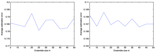
Figure 1: Averaged $\Delta(\hat{B},B_{0})$ versus ensemble size $m$ for Example 7.1. Left panel: $n=200$. Right panel: $n=400$.

versus different ensemble sizes $m$, ranging from 5 to 50. The left panel corresponds to $n=200$, and the right panel corresponds to $n=400$. We see that the average error is quite stable as $m$ varies: for $n=200$ it is between 0.1806 and 0.1922, and for $n=400$ it is between 0.1066 and 0.1086.

Example 7.2.

The following regression model is a modification of Example 3 of Wang and Xia (2008):

$$Y_{i}=\frac{X_{i1}}{0.5+(X_{i2}+1.5)^{2}}+X_{i3}\varepsilon_{i},$$

where $\varepsilon_{i}$ and $X_{i}$ are generated as in Example 7.1 with $n=400$. In this case $d_{0}=3$ and $B_{0}=(e_{1},e_{2},e_{3})\in\mathbb{R}^{p\times 3}$. We use $m=15$ for

Table 1: Comparisons for (Example 7.2). Entries are $\mbox{mean}\pm\mbox{standard error}$ of $\Delta(\hat{B}_{0},B_{0})$ calculated from 100 simulation samples

$\bolds{p}$	RMAVE-$\bolds{\mathfrak{F}_{C}}$	SR	RMAVE-$\bolds{{\mathfrak{F}_{B}}}$	RMAVE	DMAVE	SIR	SAVE
10	$0.388$	$0.513$	$0.878$	$0.750$	$0.409$	$0.851$	$0.903$
	$\mbox{$\pm$}0.134$	$\mbox{$\pm$}0.192$	$\mbox{$\pm$}0.136$	$\mbox{$\pm$}0.170$	$\mbox{$\pm$}0.153$	$\mbox{$\pm$}0.115$	$\mbox{$\pm$}0.117$
20	$0.638$	$0.844$	$0.954$	$0.880$	$0.719$	$0.947$	$0.977$
	$\mbox{$\pm$}0.150$	$\mbox{$\pm$}0.146$	$\mbox{$\pm$}0.060$	$\mbox{$\pm$}0.111$	$\mbox{$\pm$}0.159$	$\mbox{$\pm$}0.055$	$\mbox{$\pm$}0.034$

RMAVE-$\mathfrak{F}_{C}$ and the number of slices $H=5$ for SR, SIR and SAVE. Table 1 below indicates that RMAVE-$\mathfrak{F}_{C}$ is the best performer, followed by DMAVE and SR.

Example 7.3.

The following model is taken from Zhu and Zeng (2006), Example 3:

$$Y_{i}=I_{[\beta_{1}^{\top}X_{i}+\sigma\varepsilon_{i}>1]}+2I_{[\beta_{2}^{\top}X_{i}+\sigma\varepsilon_{i}>0]},$$

where $\varepsilon_{i}$ is a standard normal random variable, $\sigma=0.2$ and $X_{i}\sim N(0,I_{p})$. The regression coefficients are $\beta_{1}=e_{1}+\cdots+e_{4}$ and $\beta_{2}=e_{p-3}+\cdots+e_{p}$. Thus we have $d_{0}=2$ and $B_{0}=(\beta_{1},\beta_{2})$. The specifications for $n,m,H$ are the same as Example 7.2. Table 2 below

Table 2: Comparisons for (Example 7.3). Entries are $\mbox{mean}\pm\mbox{standard error}$ of $\Delta(\hat{B}_{0},B_{0})$ calculated from 100 simulation samples

$\bolds{p}$	RMAVE-$\bolds{\mathfrak{F}_{C}}$	SR	RMAVE-$\bolds{{\mathfrak{F}_{B}}}$	RMAVE	DMAVE	SIR	SAVE
10	$0.101$	$0.149$	$0.156$	$0.149$	$0.100$	$0.256$	$0.294$
	$\mbox{$\pm$}0.023$	$\mbox{$\pm$}0.044$	$\mbox{$\pm$}0.047$	$\mbox{$\pm$}0.041$	$\mbox{$\pm$}0.019$	$\mbox{$\pm$}0.048$	$\mbox{$\pm$}0.063$
20	$0.155$	$0.246$	$0.243$	$0.243$	$0.148$	$0.339$	$0.510$
	$\mbox{$\pm$}0.028$	$\mbox{$\pm$}0.059$	$\mbox{$\pm$}0.055$	$\mbox{$\pm$}0.098$	$\mbox{$\pm$}0.020$	$\mbox{$\pm$}0.046$	$\mbox{$\pm$}0.096$

=220pt Model $\bolds{n=100}$ $\bolds{n=200}$ $\bolds{n=400}$ A 0.95 1.00 1.00 B 0.83 1.00 1.00 C 0.39 0.60 0.79

Table 3: Percentage of correctly estimated $d_{0}$ using the CV criterion combined with RMAVE-$\mathfrak{F}_{C}$ (Example 7.4)

reports the results. In this case DMAVE is the top performer, with RMAVE-$\mathfrak{F}_{C}$ as a close second.

Example 7.4.

This example is to investigate the effectiveness of the CV criterion for order determination introduced in Section 5, as used in conjunction with RMAVE-$\mathfrak{F}_{C}$, in the spirit similar to Example 4 of Wang and Xia (2008). We consider the following three models:

$$\mbox{Model A:}\quad Y_{i} = (X_{i}^{\top}\beta)^{-1}+0.2\varepsilon_{i},\qquad\beta_{0}=e_{1}+\cdots+e_{4},$$

$$\mbox{Model B:}\quad Y_{i} = \cos(2X_{i1})-\cos(X_{i2})+0.2\varepsilon_{i},$$

$$\mbox{Model C:}\quad Y_{i} = {X_{i1}}/[0.5+(X_{i2}+1.5)^{2}]+X_{i3}^{2}\varepsilon_{i},$$

where $X$ is generated as in Example 7.1. We take $p=10$, $m=15$. Table 3 shows that, as the sample size $n$ increases, the percentages of correctly identified dimensions quickly approach to 100% for all three models, which is comparable with the results in Wang and Xia (2008). Our results for the first two models show substantial improvement over the corresponding results in Wang and Xia (2008) for $n=100$ and $n=200$. A possible explanation of this improvement is that RMAVE-$\mathfrak{F}_{C}$ allows us to make repeated use of the sample of responses, with each repetition exploring a different aspect of the central subspace. In other words the ensemble approach makes fuller use of the data than dividing them into slices.

Example 7.5.

The four models in this example are the same as those used in Example 5 of Wang and Xia (2008):

$$\mbox{Model D:}\quad Y_{i} = (X_{i}^{\top}\beta)^{-1}+0.2\varepsilon_{i},\qquad\beta=e_{1}+\cdots+e_{4};$$

$$\mbox{Model E:}\quad Y_{i} = 0.1(X_{i}^{\top}\beta+\varepsilon_{i})^{3},\qquad\beta=e_{1}+\cdots+e_{4};$$

$$\mbox{Model F:}\quad Y_{i} = \exp(X_{i}^{\top}\beta)\times\varepsilon_{i},\qquad\beta=e_{1}+0.5e_{2}+e_{3};$$

$$\mbox{Model G:}\quad Y_{i} = \operatorname{sign}(2X_{i1}+\varepsilon_{i1})\times{\log}|2X_{i2}+4+\varepsilon_{i2}|.$$

Here, $X,n,m,H$ are the same as specified in Example 7.1. Table 4 below reports the result for $n=400$.

Table 4: Comparisons for (Example 7.5). Entries are $\mbox{mean}\pm{\mbox{standard error}}$ of $\Delta(\hat{B}_{0},B_{0})$ calculated from 100 simulation samples

$\bolds{p}$	Model	RMAVE-$\bolds{\mathfrak{F}_{C}}$	SR	RMAVE-$\bolds{{\mathfrak{F}_{B}}}$	RMAVE	DMAVE	SIR	SAVE
10	D	$0.052$	$0.082$	$0.994$	$0.983$	$0.313$	$0.306$	$0.243$
		$\pm 0.014$	$\pm 0.024$	$\pm 0.008$	$\pm 0.067$	$\pm 0.412$	$\pm 0.072$	$\pm 0.075$
	E	$0.053$	$0.059$	$0.609$	$0.058$	$0.054$	$0.141$	$0.154$
		$\pm 0.016$	$\pm 0.015$	$\pm 0.173$	$\pm 0.015$	$\pm 0.014$	$\pm 0.037$	$\pm 0.040$
	F	$0.163$	$0.178$	$0.869$	$0.798$	$0.208$	$0.225$	$0.230$
		$\pm 0.043$	$\pm 0.055$	$\pm 0.979$	$\pm 0.141$	$\pm 0.073$	$\pm 0.056$	$\pm 0.067$
	G	$0.198$	$0.217$	$0.387$	$0.349$	$0.931$	$0.242$	$0.601$
		$\pm 0.053$	$\pm 0.059$	$\pm 0.178$	$\pm 0.109$	$\pm 0.084$	$\pm 0.058$	$\pm 0.230$
20	D	$0.080$	$0.122$	$0.955$	$0.996$	$0.501$	$0.399$	$0.363$
		$\pm 0.016$	$\pm 0.023$	$\pm 0.006$	$\pm 0.006$	$\pm 0.459$	$\pm 0.070$	$\pm 0.068$
	E	$0.068$	$0.092$	$0.694$	$0.085$	$0.075$	$0.179$	$0.236$
		$\pm 0.015$	$\pm 0.018$	$\pm 0.200$	$\pm 0.017$	$\pm 0.014$	$\pm 0.030$	$\pm 0.061$
	F	$0.250$	$0.281$	$0.927$	$0.879$	$0.323$	$0.303$	$0.414$
		$\pm 0.048$	$\pm 0.052$	$\pm 0.058$	$\pm 0.103$	$\pm 0.080$	$\pm 0.053$	$\pm 0.083$
	G	$0.299$	$0.321$	$0.507$	$0.535$	$0.973$	$0.312$	$0.957$
		$\pm 0.048$	$\pm 0.054$	$\pm 0.146$	$\pm 0.166$	$\pm 0.034$	$\pm 0.050$	$\pm 0.060$

We see that RMAVE-$\mathfrak{F}_{C}$ again consistently outperforms other estimators in all four models, though SR is quite close to it in some cases.

Example 7.6.

As we noted before, the family $\mathfrak{F}_{C}$ is particularly useful for recovering directions in the ${\mathcal{S}}_{Y|X}$ that do not belong to ${\mathcal{S}}_{E(Y|X)}$, and when $Y$ contains outliers. This example indicates that in the case where ${\mathcal{S}}_{Y|X}={\mathcal{S}}_{E(Y|X)}$ and $Y$ contains no outliers—conditions favorable to RMAVE. Consider the model

$$Y_{i}=\arcsin\bigl{(}1/(1+|0.5+X_{i1}|)\bigr{)}+0.2\varepsilon_{i},$$

where $\varepsilon_{i}$ and $X_{i}\in\mathbb{R}^{10}$ are generated as in Example 7.1. Note that in this case both ${\mathcal{S}}_{Y|X}$ and ${\mathcal{S}}_{E(Y|X)}$ are spanned by $e_{1}$. We take $m=15$, $n=400$ and the number of slices for SR, SIR and SAVE equal to 5. However, Table 5 indicates that RMAVE-$\mathfrak{F}_{C}$ is slightly better than RMAVE.

Example 7.7.

The main point of this example is to demonstrate numerically the $\sqrt{n}$-consistency of RMAVE-$\mathfrak{F}_{C}$, which we have shown analytically in Section 6 for $d_{0}\leq 3$. A secondary point is to reconfirm the stability of this estimator against the change of ensemble size $m$, for a wide range of sample sizes $n$, which we have demonstrated in Example 7.1 for two sample sizes ($n=200,400$). This second point also provides us intuition about the double limits, $\lim_{m\to\infty}\lim_{n\to\infty}$, we took in Section 6.

Table 5: Comparisons for (Example 7.6). Entries are $\mbox{mean}\pm\mbox{standard error}$ of $\Delta(\hat{B}_{0},B_{0})$ calculated from 100 simulation samples

$\bolds{p}$	RMAVE-$\bolds{\mathfrak{F}_{C}}$	SR	RMAVE-$\bolds{{\mathfrak{F}_{B}}}$	RMAVE	DMAVE	SIR	SAVE
10	$0.098$	$0.114$	$0.128$	$0.103$	$0.132$	$0.434$	$0.310$
	$\pm 0.023$	$\pm 0.031$	$\pm 0.035$	$\pm 0.026$	$\pm 0.031$	$\pm 0.134$	$\pm 0.086$
20	$0.131$	$0.155$	$0.180$	$0.143$	$0.207$	$0.590$	$0.547$
	$\pm 0.026$	$\pm 0.033$	$\pm 0.038$	$\pm 0.028$	$\pm 0.062$	$\pm 0.106$	$\pm 0.132$

Here we adopt the approach of Wang and Xia (2008), Example 8. We use model D in Example 7.5. In Figure 2 we plot the averaged $\Delta(\hat{B},B_{0})$

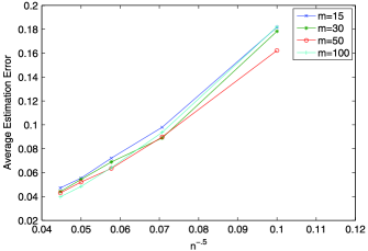
Figure 2: Numerical demonstration of $\sqrt{n}$-consistency for RMAVE-$\mathfrak{F}_{C}$, as described in Example 7.7.

against $1/\sqrt{n}$ for $m=15,30,50,100$. The value of $1/\sqrt{n}$ ranges from 0.045 to 0.1, corresponding to sample sizes $n=100,200,300,400,500$ in reverse order. We can see that the curves are roughly straight lines passing through the origin, which confirms the $\sqrt{n}$-consistency. We also see that the performance of RMAVE-$\mathfrak{F}_{C}$ is very stable as $m$ changes, across different sample sizes.

Example 7.8.

Finally, we investigate the performance of $\mathfrak{F}_{C}$ for multivariate responses. The model is taken from Li, Wen and Zhu (2008), Model 4.4. Here $p=6$, $s=5$. The predictor $X_{i}$ is generated from $N(0,I_{6})$. The error $\varepsilon_{i}$ is generated from $N(0,\Sigma)$, where $\Sigma=\operatorname{diag}(\Sigma_{1},\Sigma_{2})$, in which

$$\Sigma_{1}=\pmatrix{1&-1/2\cr-1/2&1/2},\qquad\Sigma_{2}=\pmatrix{1/2&0&0\cr 0&1/3&0\cr 0&0&1/4}.$$

The 5-dimensional response random vector $Y$ is generated as:

$$Y_{i1} = X_{i2}+{3X_{i2}}/[{0.5+(X_{i1}+1.5)^{2}}]+\varepsilon_{i},$$

$$Y_{i2} = X_{i1}+e^{0.5X_{i2}}+\varepsilon_{i2},$$

$$Y_{i3} = X_{i1}+X_{i2}+\varepsilon_{i3},$$

$$Y_{i4} = \varepsilon_{i4},$$

$$Y_{i5} = \varepsilon_{i5}.$$

For a fair comparison, we use the Frobenius norm instead of the operator norm for $\Delta(\hat{B},B_{0})$, the former of which was used by Li, Wen and Zhu (2008). Table 6 shows the results for $n=100$, averaged over 1,000 simulated samples.

=210pt PR-SIR RMAVE-$\bolds{\mathfrak{F}_{C}}$ PR-RMAVE $0.276\pm 0.088$ $0.248\pm 0.088$ $0.206\pm 0.071$

Table 6: Comparison of different estimators for multivariate $Y$ (Example 7.8, $n=100$)

The columns PR-SIR and PR-RMAVE refer to projective resampling used in conjunction with the SIR and RMAVE, respectively. See Li, Wen and Zhu (2008). The numbers in the PR-SIR column is taken from that paper. For RMAVE-$\mathfrak{F}_{C}$ we use $m=15\mbox{,}000$ random directions; for PR-RMAVE, we use 1,000 random directions.

In this case PR-RMAVE performs the best among the three estimators. Note that in this example the central subspace and the central mean subspace coincide, which is the most favorable scenario for methods derived from RMAVE.

8 Discussion

In this paper we introduce a general method for combining estimators of a family of central mean subspaces into a single estimator of the central subspace using the MAVE-type procedures as basic estimators for the central mean subspaces. Different combinations of the characterizing families and MAVE-type procedures result in a class of new estimators of the central subspace, which we call the ensemble estimators. Ensemble estimators exhaustively estimate the central subspace and are relatively easy to compute. The algorithm for estimation can be broken down into iterations of quadratic optimization steps, whose solutions have the least-square form. The ensemble estimators do not require special treatment for multivariate responses, because the characterizing nature of $\mathfrak{F}$ automatically takes into account the multivariate information in the response. Ensemble estimators allow repeated use of the available sample of responses, and by doing so enhance the estimation accuracy. They do not require dividing the sample into slices, which not only simplifies the operation but also avoid sensitivity to the number of slices. Ensemble estimators have the same convergence rates as their corresponding MAVE-type estimators. In particular, the RMAVE ensemble has the $\sqrt{n}$-rate when the structural dimension $d_{0}$ is no more than 4.

An important problem is the choice of $\mathfrak{F}$. At this stage we do not yet have a good theory to generate a universal criterion that can work across families. One theoretical difficulty in devising a general criterion to choose among different families $\mathfrak{F}$ is that different transformations of the response result in different scales that cannot be meaningfully compared. For example, if we use cross validation of prediction errors to choose among families, then we face the problem that the prediction errors in different families have different meanings. At this stage, we suspect that any general criterion capable of choosing among different families must be intrinsic to the probabilistic relation between $X$ and $Y$, as reflected in the conditional distribution of $Y$ given $X$, rather than specific to any form of transformation of the response.

Our empirical knowledge seems to indicate that bounded transformations, such as $\mathfrak{F}_{C}$ and SR, are preferable to unbounded transformations, such as power transformation (Example 2.1) and Box–Cox transformation (Example 2.4), especially when the model permits extreme values in the response. A bounded characterizing family of transformations serve the dual purposes of comprehensively describing the central subspace and decreasing the leverage of the extreme response values. In addition, the transformations in $\mathfrak{F}_{C}$ make full reuse of the data at each resampling. In this respect it is rather similar to the bootstrap, except that the resampling is done by random projection. Indeed, this is the very spirit of ensemble estimator we would like to advocate in this paper, and it is this aspect that distinguishes the ensemble estimators from other sufficient dimension reduction estimators. Finally, in the majority of examples we considered in Section 7, the $\mathfrak{F}_{C}$-ensemble estimator consistently outperforms other methods. In light of these empirical evidences, we regard the $\mathfrak{F}_{C}$-family as the overall best performer among the families we considered.

The choice of number $m$ is also important. Theorem 2.2 indicates that a large enough $m$ will guarantee the exhaustive recovering of the central subspace, regardless of the characterizing family used. In practice, however, different families require different choices of $m$. For the family $\mathfrak{F}_{C}$, we recommend to choose $m$ as large as computationally feasible, because adding a new function in $\mathfrak{F}_{C}$ amounts to reusing the data one more time. Since the functions in $\mathfrak{F}_{C}$ are bounded and smooth, the ensemble estimator is stable as more functions are included.

The general formulation of the ensemble estimators also provides a synthesis and fresh insights for many recently developed methods. In particular, it unifies the central mean subspace [Cook and Li (2002)], the central moment subspace [Yin and Cook (2002)], Fourier transform estimators [Zhu and Zeng (2006)], dMAVE [Xia (2007)] and sliced regression [Wang and Xia (2008)] in a coherent system. Although in this paper we have focussed on MAVE ensemble and its variations, the ensemble approach can potentially be combined with any estimator of the central mean subspaces to recover the central subspace, such as the OLS [Li and Duan (1989), Duan and Li (1991)], pHd [Li (1992), Cook (1998)] and Iterative Hessian Transformations [Cook and Li (2002, 2004)].

Finally, the ensemble approach can also be used with other characterizing families which we cannot fully explore within this paper, but which may be especially useful for some applications. One example is the wavelet basis, such as the Haar basis briefly described in Example 2.6. Such families are highly effective for handling response variables that have sharp discontinuities, which frequently arise in image analysis and pattern recognition [Donoho and Johnstone (1994)]. We leave further exploration of these possibilities to future research.

References

- Antoniadis and Fan (2001) {barticle}[mr] \bauthor\bsnmAntoniadis, \bfnmAnestis\binitsA. and \bauthor\bsnmFan, \bfnmJianqing\binitsJ. (\byear2001). \btitleRegularization of wavelet approximations. \bjournalJ. Amer. Statist. Assoc. \bvolume96 \bpages939–955. \bptokimsref \endbibitem
- Bickel and Doksum (1981) {barticle}[mr] \bauthor\bsnmBickel, \bfnmPeter J.\binitsP. J. and \bauthor\bsnmDoksum, \bfnmKjell A.\binitsK. A. (\byear1981). \btitleAn analysis of transformations revisited. \bjournalJ. Amer. Statist. Assoc. \bvolume76 \bpages296–311. \bidissn=0162-1459, mr=0624332 \bptokimsref \endbibitem
- Box and Cox (1964) {barticle}[mr] \bauthor\bsnmBox, \bfnmG. E. P.\binitsG. E. P. and \bauthor\bsnmCox, \bfnmD. R.\binitsD. R. (\byear1964). \btitleAn analysis of transformations. \bjournalJ. Roy. Statist. Soc. Ser. B \bvolume26 \bpages211–252. \bidissn=0035-9246, mr=0192611 \bptokimsref \endbibitem
- Cook (1994) {binproceedings}[auto:STB—2011/12/30—12:36:46] \bauthor\bsnmCook, \bfnmR. D.\binitsR. D. (\byear1994). \btitleUsing dimension reduction subspaces to identify important inputs in models of physical systems. In \bbooktitleProceedings of the Section on Physical and Engineering Sciences \bpages18–25. \bpublisherAmer. Statist. Assoc., \baddressAlexandra, VA. \bptokimsref \endbibitem
- Cook (1996) {barticle}[mr] \bauthor\bsnmCook, \bfnmR. Dennis\binitsR. D. (\byear1996). \btitleGraphics for regressions with a binary response. \bjournalJ. Amer. Statist. Assoc. \bvolume91 \bpages983–992. \bidissn=0162-1459, mr=1424601 \bptokimsref \endbibitem
- Cook (1998) {barticle}[mr] \bauthor\bsnmCook, \bfnmR. Dennis\binitsR. D. (\byear1998). \btitlePrincipal Hessian directions revisited (with discussion). \bjournalJ. Amer. Statist. Assoc. \bvolume93 \bpages84–100. \bidissn=0162-1459, mr=1614584 \bptokimsref \endbibitem
- Cook and Li (2002) {barticle}[mr] \bauthor\bsnmCook, \bfnmR. Dennis\binitsR. D. and \bauthor\bsnmLi, \bfnmBing\binitsB. (\byear2002). \btitleDimension reduction for conditional mean in regression. \bjournalAnn. Statist. \bvolume30 \bpages455–474. \biddoi=10.1214/aos/1021379861, issn=0090-5364, mr=1902895 \bptokimsref \endbibitem
- Cook and Li (2004) {barticle}[mr] \bauthor\bsnmCook, \bfnmR. Dennis\binitsR. D. and \bauthor\bsnmLi, \bfnmBing\binitsB. (\byear2004). \btitleDetermining the dimension of iterative Hessian transformation. \bjournalAnn. Statist. \bvolume32 \bpages2501–2531. \biddoi=10.1214/009053604000000661, issn=0090-5364, mr=2153993 \bptokimsref \endbibitem
- Cook and Weisberg (1991) {barticle}[mr] \bauthor\bsnmCook, \bfnmR. D.\binitsR. D. and \bauthor\bsnmWeisberg, \bfnmS.\binitsS. (\byear1991). \btitleDiscussion of “Sliced inverse regression for dimension reduction,” by K. C. Li. \bjournalJ. Amer. Statist. Assoc. \bvolume86 \bpages328–332. \bptokimsref \endbibitem
- Donoho and Johnstone (1994) {barticle}[mr] \bauthor\bsnmDonoho, \bfnmDavid L.\binitsD. L. and \bauthor\bsnmJohnstone, \bfnmIain M.\binitsI. M. (\byear1994). \btitleIdeal spatial adaptation by wavelet shrinkage. \bjournalBiometrika \bvolume81 \bpages425–455. \biddoi=10.1093/biomet/81.3.425, issn=0006-3444, mr=1311089 \bptokimsref \endbibitem
- Duan and Li (1991) {barticle}[mr] \bauthor\bsnmDuan, \bfnmNaihua\binitsN. and \bauthor\bsnmLi, \bfnmKer-Chau\binitsK.-C. (\byear1991). \btitleSlicing regression: A link-free regression method. \bjournalAnn. Statist. \bvolume19 \bpages505–530. \biddoi=10.1214/aos/1176348109, issn=0090-5364, mr=1105834 \bptokimsref \endbibitem
- Fan, Yao and Cai (2003) {barticle}[mr] \bauthor\bsnmFan, \bfnmJianqing\binitsJ., \bauthor\bsnmYao, \bfnmQiwei\binitsQ. and \bauthor\bsnmCai, \bfnmZongwu\binitsZ. (\byear2003). \btitleAdaptive varying-coefficient linear models. \bjournalJ. R. Stat. Soc. Ser. B Stat. Methodol. \bvolume65 \bpages57–80. \biddoi=10.1111/1467-9868.00372, issn=1369-7412, mr=1959093 \bptokimsref \endbibitem
- Fukumizu, Bach and Jordan (2009) {barticle}[mr] \bauthor\bsnmFukumizu, \bfnmKenji\binitsK., \bauthor\bsnmBach, \bfnmFrancis R.\binitsF. R. and \bauthor\bsnmJordan, \bfnmMichael I.\binitsM. I. (\byear2009). \btitleKernel dimension reduction in regression. \bjournalAnn. Statist. \bvolume37 \bpages1871–1905. \biddoi=10.1214/08-AOS637, issn=0090-5364, mr=2533474 \bptokimsref \endbibitem
- John and Draper (1980) {barticle}[auto:STB—2011/12/30—12:36:46] \bauthor\bsnmJohn, \bfnmJ. A.\binitsJ. A. and \bauthor\bsnmDraper, \bfnmN. R.\binitsN. R. (\byear1980). \btitleAn alternative family of transformations. \bjournalJ. Appl. Stat. \bvolume29 \bpages190–197. \bptokimsref \endbibitem
- Li (1991) {barticle}[mr] \bauthor\bsnmLi, \bfnmKer-Chau\binitsK.-C. (\byear1991). \btitleSliced inverse regression for dimension reduction. \bjournalJ. Amer. Statist. Assoc. \bvolume86 \bpages316–342. \bidissn=0162-1459, mr=1137117 \bptokimsref \endbibitem
- Li (1992) {barticle}[mr] \bauthor\bsnmLi, \bfnmKer-Chau\binitsK.-C. (\byear1992). \btitleOn principal Hessian directions for data visualization and dimension reduction: Another application of Stein’s lemma. \bjournalJ. Amer. Statist. Assoc. \bvolume87 \bpages1025–1039. \bidissn=0162-1459, mr=1209564 \bptokimsref \endbibitem
- Li and Duan (1989) {barticle}[mr] \bauthor\bsnmLi, \bfnmKer-Chau\binitsK.-C. and \bauthor\bsnmDuan, \bfnmNaihua\binitsN. (\byear1989). \btitleRegression analysis under link violation. \bjournalAnn. Statist. \bvolume17 \bpages1009–1052. \biddoi=10.1214/aos/1176347254, issn=0090-5364, mr=1015136 \bptokimsref \endbibitem
- Li, Wen and Zhu (2008) {barticle}[mr] \bauthor\bsnmLi, \bfnmBing\binitsB., \bauthor\bsnmWen, \bfnmSongqiao\binitsS. and \bauthor\bsnmZhu, \bfnmLixing\binitsL. (\byear2008). \btitleOn a projective resampling method for dimension reduction with multivariate responses. \bjournalJ. Amer. Statist. Assoc. \bvolume103 \bpages1177–1186. \biddoi=10.1198/016214508000000445, issn=0162-1459, mr=2462891 \bptokimsref \endbibitem
- Li, Zha and Chiaromonte (2005) {barticle}[mr] \bauthor\bsnmLi, \bfnmBing\binitsB., \bauthor\bsnmZha, \bfnmHongyuan\binitsH. and \bauthor\bsnmChiaromonte, \bfnmFrancesca\binitsF. (\byear2005). \btitleContour regression: A general approach to dimension reduction. \bjournalAnn. Statist. \bvolume33 \bpages1580–1616. \biddoi=10.1214/009053605000000192, issn=0090-5364, mr=2166556 \bptokimsref \endbibitem
- Manly (1976) {barticle}[auto:STB—2011/12/30—12:36:46] \bauthor\bsnmManly, \bfnmB. F.\binitsB. F. (\byear1976). \btitleExponential data transformation. \bjournalThe Statistician \bvolume25 \bpages37–42. \bptokimsref \endbibitem
- Scott (1992) {bbook}[mr] \bauthor\bsnmScott, \bfnmDavid W.\binitsD. W. (\byear1992). \btitleMultivariate Density Estimation: Theory, Practice, and Visualization. \bpublisherWiley, \baddressNew York. \biddoi=10.1002/9780470316849, mr=1191168 \bptokimsref \endbibitem
- Wang and Xia (2008) {barticle}[mr] \bauthor\bsnmWang, \bfnmHansheng\binitsH. and \bauthor\bsnmXia, \bfnmYingcun\binitsY. (\byear2008). \btitleSliced regression for dimension reduction. \bjournalJ. Amer. Statist. Assoc. \bvolume103 \bpages811–821. \biddoi=10.1198/016214508000000418, issn=0162-1459, mr=2524332 \bptokimsref \endbibitem
- Xia (2007) {barticle}[mr] \bauthor\bsnmXia, \bfnmYingcun\binitsY. (\byear2007). \btitleA constructive approach to the estimation of dimension reduction directions. \bjournalAnn. Statist. \bvolume35 \bpages2654–2690. \biddoi=10.1214/009053607000000352, issn=0090-5364, mr=2382662 \bptokimsref \endbibitem
- Xia et al. (2002) {barticle}[mr] \bauthor\bsnmXia, \bfnmYingcun\binitsY., \bauthor\bsnmTong, \bfnmHowell\binitsH., \bauthor\bsnmLi, \bfnmW. K.\binitsW. K. and \bauthor\bsnmZhu, \bfnmLi-Xing\binitsL.-X. (\byear2002). \btitleAn adaptive estimation of dimension reduction space (with discussion). \bjournalJ. R. Stat. Soc. Ser. B Stat. Methodol. \bvolume64 \bpages363–410. \biddoi=10.1111/1467-9868.03411, issn=1369-7412, mr=1924297 \bptokimsref \endbibitem
- Yin and Cook (2002) {barticle}[mr] \bauthor\bsnmYin, \bfnmXiangrong\binitsX. and \bauthor\bsnmCook, \bfnmR. Dennis\binitsR. D. (\byear2002). \btitleDimension reduction for the conditional th moment in regression. \bjournalJ. R. Stat. Soc. Ser. B Stat. Methodol. \bvolume64 \bpages159–175. \biddoi=10.1111/1467-9868.00330, issn=1369-7412, mr=1904698 \bptokimsref \endbibitem
- Yin, Li and Cook (2008) {barticle}[mr] \bauthor\bsnmYin, \bfnmXiangrong\binitsX., \bauthor\bsnmLi, \bfnmBing\binitsB. and \bauthor\bsnmCook, \bfnmR. Dennis\binitsR. D. (\byear2008). \btitleSuccessive direction extraction for estimating the central subspace in a multiple-index regression. \bjournalJ. Multivariate Anal. \bvolume99 \bpages1733–1757. \biddoi=10.1016/j.jmva.2008.01.006, issn=0047-259X, mr=2444817 \bptokimsref \endbibitem
- Zeng and Zhu (2010) {barticle}[mr] \bauthor\bsnmZeng, \bfnmPeng\binitsP. and \bauthor\bsnmZhu, \bfnmYu\binitsY. (\byear2010). \btitleAn integral transform method for estimating the central mean and central subspaces. \bjournalJ. Multivariate Anal. \bvolume101 \bpages271–290. \biddoi=10.1016/j.jmva.2009.08.004, issn=0047-259X, mr=2557633 \bptokimsref \endbibitem
- Zhu and Zeng (2006) {barticle}[mr] \bauthor\bsnmZhu, \bfnmYu\binitsY. and \bauthor\bsnmZeng, \bfnmPeng\binitsP. (\byear2006). \btitleFourier methods for estimating the central subspace and the central mean subspace in regression. \bjournalJ. Amer. Statist. Assoc. \bvolume101 \bpages1638–1651. \biddoi=10.1198/016214506000000140, issn=0162-1459, mr=2279485 \bptokimsref \endbibitem
- Zhu and Zhu (2009) {barticle}[mr] \bauthor\bsnmZhu, \bfnmLi-Ping\binitsL.-P. and \bauthor\bsnmZhu, \bfnmLi-Xing\binitsL.-X. (\byear2009). \btitleDimension reduction for conditional variance in regressions. \bjournalStatist. Sinica \bvolume19 \bpages869–883. \bidissn=1017-0405, mr=2514192 \bptokimsref \endbibitem