Generalized Elastic Model yields Fractional Langevin Equation

Abstract

Starting from a generalized elastic model which accounts for the stochastic motion of several physical systems such as membranes, (semi)flexible polymers and fluctuating interfaces among others, we derive the fractional Langevin equation (FLE) for a probe particle in such systems, in the case of thermal initial conditions. We show that this FLE is the only one fulfilling the fluctuation-dissipation (FD) relation within a new family of fractional Brownian motion (FBM) equations. The FLE for the time-dependent fluctuations of the donor-acceptor distance in a protein, is shown to be recovered. When the system starts from non-thermal conditions, the corresponding FLE, which does not fulfill FD relation, is derived.

Introduction.– Continuum elastic models have been extensively used in statistical mechanics to study the dynamics of real physical systems. Examples include: (semi)flexible polymers  Granek ; semiflexible ; Doi , membranes  membranes ; membranes-FLE ; Granek ; Zilman , growing interfaces interfaces ; Krug ; Edwards ; Gao ; DeGennes , fluctuating surfaces surfaces and diffusion-noise systems  VKampen . In this paper we consider the following Markovian equation for a generalization of the accounted elastic models (generalized elastic model)

$$\frac{\partial}{\partial t}\mathbf{h}\left(\vec{x},t\right)=\int d^{d}x^{\prime}\Lambda\left(\vec{x}-\vec{x}^{\prime}\right)\frac{\partial^{z}}{\partial\left|\vec{x}^{\prime}\right|^{z}}\mathbf{h}(\vec{x}^{\prime},t)+\boldsymbol{\eta}\left(\vec{x},t\right)$$ (1)

for the dynamics of the $D$-dimensional stochastic process $\mathbf{h}$ in the $d-$dimensional infinite space: the internal $d$ coordinates are represented by $\vec{x}$ and the Gaussian white noise satisfies the fluctuation-dissipation (FD) relation

$$\langle\eta_{j}\left(\vec{x},t\right)\eta_{k}\left(\vec{x}^{\prime},t^{\prime}\right)\rangle=2k_{B}T\Lambda\left(\vec{x}-\vec{x}^{\prime}\right)\delta_{j\,k}\delta(t-t^{\prime}).$$ (2)

with $j,k\in[1,D]$. The Riesz fractional operator is defined via its Fourier transform as ${\cal F}_{\vec{q}}\left\{\frac{\partial^{z}}{\partial\left|\vec{x}\right|^{z}}\right\}\equiv-\left|\vec{q}\right|^{z}$ ($z>0$)  Zazlawsky or, in terms of the Laplacian $\Delta$, as $\frac{\partial^{z}}{\partial\left|\vec{x}\right|^{z}}:=-\left(-\Delta\right)^{z/2}$  Samko . In the following analysis we study two classes of hydrodynamic interactions: long ranged, $\Lambda\left(\vec{r}\right)\sim\left|\vec{r}\right|^{-\alpha}$ as $\vec{r}\to\infty$, with $0<\alpha<d$, and local, $\Lambda\left(\vec{r}\right)=\delta^{d}\left(\vec{r}\right)$. In the non-local case, if $\alpha=d$ we take $\Lambda\left(\vec{r}\right)\sim\frac{1}{a+\left|\vec{r}\right|^{d}}$ where $a$ is a microscopic cutoff.

Long range hydrodynamic interactions. The hydrodynamic interactions are often represented by the equilibrium average of the Oseen tensor, which in an embedding $d_{e}$-dimensional space ($d_{e}\geq 3$) reads  Doi : $\Lambda\left(\vec{r}\right)\sim\left|\vec{r}\right|^{2-d_{e}}$. Examples are: (I) fluid membranes  membranes ; membranes-FLE ; Granek ; Zilman , whose height $h\left(\vec{x},t\right)$ of a point $\vec{x}$ on the 2-dimensional (planar) base surface is moving in time according to (1), with $\alpha=D+d-2=1$ and $z=4$ as derived from the Helfrich bending free energy for small deformations  Helfrich . (II) Semiflexible and flexible polymers’ models, where $\mathbf{h}$ represents the 3 spatial coordinates of a polymeric segment (bead), while $x$ is the strand’s 1-dimensional internal coordinate (curvilinear abscissa). For semiflexible filaments  Granek ; semiflexible the bending elastic energy associated with the chain’s deformation implies $z=4$  Harris and from the Oseen tensor formula we get $\alpha=D-2=1$; for the flexible polymers, often referred to as Zimm model  Doi , the free energy contribution solely comes from the elastic term, i.e. $z=2$, and $\alpha=1/2$ in $\Theta$ solvent.

Local hydrodynamic interactions. Examples of the case where hydrodynamic interactions are completely screened out are: (I) the Rouse model equation for polymer dynamics  Doi , once one sets $D=3$, $d=1$ and $z=2$. (II) Single file system: recently it has been shown  single_file that the dynamics of a gas of Brownian hard rods on a line can be mapped onto the harmonic chain problem ($z=2$), where $h(x,t)$ stands for the position of the $x$-th particle on the 1-dimensional substrate at time $t$. (III) Fluctuating interfaces  interfaces ; Krug , where $h$ plays the role of a scalar field (mostly the height of a rough surface in $d$ dimension) which is subjected to a non-standard elastic force embodied by the fractional derivative of order $z$. This is actually the generalization of the Edwards-Wilkinson equation for the fluctuating profile of a granular surface, for which $d=2$, $z=2$  Edwards . In systems such as crack propagation  Gao and contact line of a liquid meniscus  DeGennes $d=1$ and the restoring forces are characterized by $z=1$. If instead $h$ is meant to be a step, namely a line boundary at which the surface changes height by one or more atomic units, the value of $z$ in eq.(1) is found to be $z=2,3$ or $4$ ($d=1$) according to the character of the atomic diffusion  surfaces . (IV) Diffusion-noise equation  VKampen : in this case $h$ represents the density field on a $d$-dimensional surface $\vec{x}$ and $z=2$.

The aim of this manuscript is to derive the non-Markovian time-FLE for the field $h_{j}$ at a given position $\vec{x}$ (probe particle), given that the whole system’s dynamics obeys the space fractional Markovian equation (1). We interpret the FLE as a particular case of a broader class of stochastic equations for FBM, i.e. the generalized fractional Langevin equation.

Autocorrelation function.– We hereby calculate the $h$-autocorrelation function $\langle\delta h\left(\vec{x},t\right)\delta h\left(\vec{x},t^{\prime}\right)\rangle=\langle\left[h_{j}\left(\vec{x},t\right)-h_{j}\left(\vec{x},0\right)\right]\left[h_{j}\left(\vec{x},t^{\prime}\right)-h_{j}\left(\vec{x},0\right)\right]\rangle$. Defining the Fourier transform in space and time as $h_{j}\left(\vec{q},\omega\right)=\int d^{d}x\,dt\,e^{-i(\vec{q}\cdot\vec{x}-\omega t)}h_{j}\left(\vec{x},t\right)$, the solution of (1) is

$$h_{j}\left(\vec{q},\omega\right)=\frac{\eta_{j}\left(\vec{q},\omega\right)}{-i\omega+\Lambda\left(\vec{q}\right)\left|\vec{q}\right|^{z}},$$ (3)

where $\Lambda\left(\vec{q}\right)$ stands for the $d$-dimensional Fourier transform of the hydrodynamic interaction term, reading $\Lambda\left(\vec{q}\right)=\frac{(4\pi)^{d/2}}{2^{\alpha}}\frac{\Gamma\left((d-\alpha)/2\right)}{\Gamma\left(\alpha/2\right)}\left|\vec{q}\right|^{\alpha-d}=A\left|\vec{q}\right|^{\alpha-d}$; if $\alpha=d$ in first approximation we can neglect the logarithmic corrections in the hydrodynamic term’s Fourier transform  Granek , i.e. $\Lambda\left(\vec{q}\right)\sim const$. In the local hydrodynamic situation $\Lambda\left(\vec{q}\right)=1$, which corresponds to put $A=1$ and $\alpha=d$ in the long-ranged hydrodynamic expression: this substitution (which is not to be intended as a limit) allows us to easily shift from power-law to local hydrodynamics throughout the following analysis. Moreover, due to the isotropy of the problem under study, we can drop the label $j$ in (3). The $h$-autocorrelation function is readily obtained: the general expression looks like

$$\langle\delta h\left(\vec{x},t\right)\delta h\left(\vec{x},t^{\prime}\right)\rangle=K\left[t^{\beta}+t^{\prime\beta}-\left|t-t^{\prime}\right|^{\beta}\right]$$ (4)

where the anomlaous diffusion exponent $\beta$ and the diffusion constant $K$ are defined as

$$\left\{\begin{array}[]{l}\beta=\frac{z-d}{\alpha+z-d}\\ K=\frac{2k_{B}T\pi^{d/2}}{(2\pi)^{d}\Gamma\left(d/2\right)}\frac{A^{\beta}\Gamma\left(1-\beta\right)}{z-d}.\end{array}\right.$$ (5)

Henceforth we will concentrate on the case $z>d$, which does not need any regularization of the $\vec{q}$ integrals in the inverse Fourier transform. The cases $z<d$ and $z=d$ will be reported elsewhere. From (4) it is apparent that the probe particle placed at a given $\vec{x}$ performs a fractional Brownian motion (FBM) which is always subdiffusive, namely $\langle\delta^{2}h\left(\vec{x},t\right)\rangle=2Kt^{\beta}$.

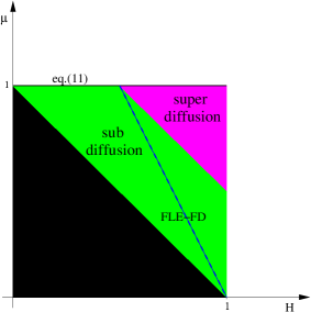
Figure 1: (Color online) Schematic picture of the GFLE ($\mu,H$) parameter space.

Fractional Langevin Equation.– We now proceed to derive the fractional Langevin equation (FLE) for a probe particle placed at position $\vec{x}$, which fulfills the FD relation. In what follows we show that this is the only fractional stochastic equation physically relevant for the considered system (1). We first include long-ranged hydrodynamic interactions. We multiply both sides of the Fourier solution (3) by $K^{+}(-i\omega)^{\beta}$, where $K^{+}=\frac{k_{B}T}{K}\,\frac{1}{\Gamma\left(1+\beta\right)}.$ We then define the following function

$$\Phi\left(\vec{x},\omega\right)=\int\frac{d^{d}q}{(2\pi)^{d}}\frac{e^{-i\vec{q}\cdot\vec{x}}\,(-i\omega)^{\beta}}{-i\omega+A\left|\vec{q}\right|^{z+\alpha-d}}.$$ (6)

Inverting the Fourier transforms in space gives

$$(-i\omega)^{\beta}K^{+}h\left(\vec{x},\omega\right)=\zeta\left(\vec{x},\omega\right)$$ (7)

where we have introduced the fractional Gaussian noise (fGN) $\zeta\left(\vec{x},\omega\right)=K^{+}\int d^{d}x^{\prime}\,\eta\left(\vec{x}-\vec{x}^{\prime},\omega\right)\Phi\left(\vec{x}^{\prime},\omega\right)$. In time domain the previous equation takes the final form of a FLE  Lutz ; single_file ; Taloni ; Kou ; membranes-FLE :

$$K^{+}D_{+}^{\beta}h\left(\vec{x},t\right)=\zeta\left(\vec{x},t\right),$$ (8)

where $D_{+}^{\beta}$ is the Caputo derivative defined as  Samko ; Podlubny

$$D_{+}^{\beta}f(t)=\frac{1}{\Gamma\left(1-\beta\right)}\int_{-\infty}^{t}dt^{\prime}\frac{1}{\left(t-t^{\prime}\right)^{\beta}}\frac{d}{dt^{\prime}}f\left(t^{\prime}\right),\ \ 0<\beta<1.$$ (9)

The noise in (8) can be shown to satisfy the FD relation,

$$\langle\zeta\left(\vec{x},t\right)\zeta\left(\vec{x},t^{\prime}\right)\rangle=k_{B}T\frac{K^{+}}{\Gamma\left(1-\beta\right)\left|t-t^{\prime}\right|^{\beta}}.$$ (10)

In the absence of any hydrodynamic interaction the anomalous diffusion exponent $\beta$ in (8) and (10) is $\beta=1-d/z$  Krug . Along these lines, the FLE for the case $d=1,\,z=2,\,\Lambda\left(x-x^{\prime}\right)=\delta\left(x-x^{\prime}\right)$ has been obtained in  single_file : our derivation can thus be viewed as a generalization of the technique used in such model. We emphasize that the spatial correlations appearing in the model (1) are translated into time correlations described by the fractional derivative (9), together with the space-time correlations of the noise $\zeta\left(\vec{x},t\right)$. As a consequence, any $h$-correlation function can be calculated starting from (8), e.g. $\langle\left[h\left(\vec{x},t\right)-h\left(\vec{x^{\prime}},0\right)\right]^{2}\rangle$ has been studied for fluctuating membranes  Zilman . We note that the underlying assumption in the expression (8) is that the system has reached the thermal equilibrium at $t=0$ and the system’s configuration is drawn from the stationary Gibbsian probability distribution $\sim e^{-\frac{1}{2\,k_{B}T}\int{d\vec{x}\left(\frac{\partial^{z/2}h\left(\vec{x},0\right)}{\partial\left|\vec{x}\right|^{z/2}}\right)^{2}}}$  Santachiara .

Now, it is possible to recast the result (10) in the same fashion as the fGn correlation function of a FBM  Mandelbroot : $\langle\zeta_{H}\left(t\right)\zeta_{H}\left(t^{\prime}\right)\rangle\propto\left|t-t^{\prime}\right|^{2H-2}$, with $H=1-\frac{\beta}{2}$. It stems from (4) and (5) that the $h$-autocorrelation function can be expressed as $\langle\delta h\left(\vec{x},t\right)\delta h\left(\vec{x},t^{\prime}\right)\rangle\propto t^{2-2H}+t^{\prime 2-2H}-\left|t-t^{\prime}\right|^{2-2H}$, which is at odd with the corresponding standard FBM quantity  Mandelbroot , whose the exponent is $2H$. However this is not surprising, since the two processes obey two different stochastic fractional equations: i) the FLE (8) for systems which fulfill the FD relation, and ii) the usual equation

$$\frac{dB_{H}(t)}{dt}=\zeta_{H}\left(t\right)$$ (11)

for FBM  Mandelbroot .

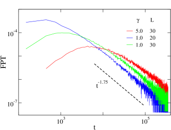
Figure 2: (Color online) First passage time (FPT) distribution of the tagged single file particle initially placed at distance L from the adsorbing boundary. The system consists of $2\times 10^{4}$ Brownian particles subjected to hard-core interaction. Simulation’ details can be found in  single_file ; Taloni . The parameters are: the file’s particle density $\rho=0.25$, the temperature $k_{B}T=1$ and the damping $\gamma$. The theoretical prediction $\sim t^{-1.75}$ has been drawn for the reader convenience (dashed line).

Generalized Fractional Langevin Equation.– Let us now generalize eq.(8) and (11). Consider a stochastic process $G(t)$ governed by the following dynamical equation

$$D_{+}^{\mu}G(t)=\zeta_{H}\left(t\right)$$ (12)

where $\zeta_{H}\left(t\right)$ is a fGn which satisfies $\langle\zeta_{H}\left(t\right)\rangle=0$ and $\langle\zeta_{H}\left(t\right)\zeta_{H}\left(t^{\prime}\right)\rangle\simeq C\left|t-t^{\prime}\right|^{2H-2}$ for $\left|t-t^{\prime}\right|\to\infty$ with $0<H<1$, $H\neq 1/2$; $C<0$ if $0<H<1/2$, and $C>0$ if $1/2<H<1$. For $H=1/2$ ($C>0$) $\zeta_{H}\left(t\right)$ is the white Gaussian noise  Kobelev . The fractional derivative has been defined in (9): it is immediate to recover equation (11) in the limiting case $\mu=1$, once that $D_{+}^{1}=d/dt$ and $C=2H(2H-1)$, and also the FLE (8), setting $K^{+}=1$, for systems satisfying the FD relation: $\mu=2-2H$ and $C=k_{B}T/\Gamma(2H-1)$. The autocorrelation function can be calculated to yield

$$\langle\delta G\left(t\right)\delta G\left(t^{\prime}\right)\rangle=\frac{C\sin\left(\pi H\right)\Gamma\left(2H-1\right)}{\sin\left(\pi\left(H+\mu-1\right)\right)\Gamma\left(2H+2\mu-1\right)}\times$$

$$\ \ \times\left[t^{2(H+\mu-1)}+t^{\prime 2(H+\mu-1)}-\left|t-t^{\prime}\right|^{2(H+\mu-1)}\right].$$ (13)

Expression (13) shows that $G(t)$ is a FBM with Hurst exponent $H_{FBM}=H+\mu-1$ ($1<H+\mu<2$  footnote ). As a consequence, systems for which $H+\mu<3/2$ exhibit subdiffusive motion, which instead is superdiffusive for $H+\mu>3/2$. It is interesting to note that the class of FBM for which the FD relation holds can be only subdiffusive. These results are summarized in Fig.[1].

An important corollary of (13) states that any statistical property which is shown to be valid for a given pair of values $\mu^{\prime}$ and $H^{\prime}$, is automatically valid for any other pair ($\mu^{\prime\prime},\,H^{\prime\prime}$) which satisfies $\mu^{\prime}+H^{\prime}=\mu^{\prime\prime}+H^{\prime\prime}$. The demonstration is straightforward: it is sufficient to note that, since $G(t)$ is a Gaussian process, it is fully specified by the correlation function (13). As an example, take the first passage time distribution (FPT) in a semi-infinite domain for a FBM, which decays asymptotically like $\sim t^{H_{FBM}-2}$  Krug ; Molchan . We immediately get that the FPT distribution for a process which is solution of (12) is given by $\sim t^{\mu+H-3}$, which in turn reads $\sim t^{\frac{\beta}{2}-2}$ for systems obeying to (1). We numerically support this result as shown in Fig.[2]. The FPT distribution of a tagged particle in single file system, which has been shown to be described by a FLE with $H=3/4$  single_file ; Taloni , since $\mu=2-2H$, attains the $\sim t^{-1.75}$ asymptotic behavior.

On the other hand, given an FBM process with $\langle\delta^{2}G(t)\rangle\sim t^{2H_{FBM}}$, there is no chance to determine the correct pair $(\mu,H)$ among the GFLEs (12) for which $\mu+H-1=H_{FBM}$. Nevertheless, introducing an external potential does the trick: for instance, adding a constant force $F$ on the right-hand side of (12) gives $\langle G(t)\rangle=F\frac{t^{\mu}}{\Gamma(\mu+1)}$, while an harmonic force $-\Omega^{2}G(t)$ leads to the relaxation $\langle G(t)\rangle/G(0)=\langle G(t)G(0)\rangle/\langle G^{2}(0)\rangle\to E_{\mu,1}\left[-\left(t/t_{0}\right)^{\mu}\right]$, in case of deterministic and thermal initial conditions respectively, where $t_{0}=\Omega^{-2/\mu}$ and $E_{\mu,\nu}$ stands for the Mittag-Leffler function  Podlubny .

One might question the uniqueness of the FLE (8) among the whole family of GFLEs for the probe particle $h\left(\vec{x},t\right)$. It is possible to show that eq.(8) is the unique GFLE for a process $h\left(\vec{x},t\right)$ whose dynamics is ruled by eq.(1). The demonstration deals with the introduction of a local constant force field $F_{j}\delta\left(\vec{x}-\vec{x}^{\star}\right)\theta(t)$ on the right-hand side of eq.(1). Since the system fulfills the FD relation (2), the connection between the average drift of $h\left(\vec{x}^{\star},t\right)$ and its mean square displacement in the absence of force is given by the Einstein relation

$$\langle h\left(\vec{x}^{\star},t\right)\rangle_{F}=F\frac{\langle\delta^{2}h\left(\vec{x}^{\star},t\right)\rangle}{2k_{B}T}.$$ (14)

The only GFLE which reproduces (14) is that which preserves the FD relation, i.e. the FLE (8).

Let’s now briefly discuss a practical example of the usefulness of the framework developed here. In Refs Kou ; Min Sunny Xie and coworkers succeeded in modeling the motion of the donor-acceptor (D-A) distance within a protein, as the coordinate of a fictitious particle diffusing in an harmonic potential according to a FLE with fractional derivative of order 1/2. In the spirit of Refs Tang ; Debnath , we consider an idealized Rouse chain as a model for the protein conformational dynamics. Therefore we take $D=3,\,d=1,\,z=2$ and $\Lambda\left(x-x^{\prime}\right)=\delta\left(x-x^{\prime}\right)$ in (1). The D-A distance vector can be expressed as $\mathbf{\Delta}_{D-A}(t)=\mathbf{h}\left(x_{A},t\right)-\mathbf{h}\left(x_{D},t\right)$, and its correlation function by  Debnath $\langle\mathbf{\Delta}_{D-A}(t)\cdot\mathbf{\Delta}_{D-A}(t^{\prime})\rangle=3\langle\Delta_{D-A}(t)\Delta_{D-A}(t^{\prime})\rangle$ due to the isotropy of the system. Hence, we can employ the result of Ref. single_file , which shows that the generalized Langevin equation for the single component $\Delta_{D-A}(t)$ is $1/2\,D_{+}^{1/2}\Delta_{D-A}(t)=-\omega^{2}_{0}\left[\Delta_{D-A}(t)-\Delta_{D-A}(0)\right]+\zeta_{D-A}(t)$ in the long time limit , with $\omega_{0}\propto(x_{A}-x_{D})^{-1/2}$ and $\zeta_{D-A}(t)$ satisfying the FD relation. However we point out here again that $\langle\Delta_{D-A}(t)\Delta_{D-A}(t^{\prime})\rangle$ can be evaluated directly from eq.(8).

Non-thermal initial conditions.– Let’s now assume that the initial conditions for the system in (1) are given by

$$h\left(\vec{x},0\right)=0$$ (15)

without loss of generality. For systems such as fluctuating interfaces  interfaces ; Krug ; Edwards ; surfaces or membranes  membranes ; membranes-FLE ; Granek ; Zilman , eq.(15) assumes the interface to be flat at $t=0$. In the case of a polymer, we can imagine eq.(15) to be valid only for the $j$-th component, achieving an initial configuration which is randomly arranged within the plane $j=0$. For single file systems eq.(15) consists of taking particles equally spaced at $t=0$. The $h$-autocorrelation function can be obtained in the same fashion as in the case of thermal initial conditions by using Laplace transform in time instead of the Fourier transform. A straightforward calculation yields

$$\langle\delta h\left(\vec{x},t\right)\delta h\left(\vec{x},t^{\prime}\right)\rangle=K\left[\left(t+t^{\prime}\right)^{\beta}-\left|t-t^{\prime}\right|^{\beta}\right]$$ (16)

where the value of $K$ and $\beta$ get the same expressions as in (5). For local hydrodynamics eq.(16) matches the result previously obtained by Krug et al. for fluctuating interfaces  Krug .

It is easy to show that the FLE expression (8) is still valid, with the Caputo derivative having its lower terminal at $t=0$  Caputo ; Podlubny . When attempting to recover the FD relation, however, one gets the following form of the noise correlation function

$$\langle\zeta\left(\vec{x},t\right)\zeta\left(\vec{x},t^{\prime}\right)\rangle=\frac{k_{B}T\,K^{+}}{\Gamma\left(1-\beta\right)}\left[\left|t-t^{\prime}\right|^{-\beta}-\left(t+t^{\prime}\right)^{-\beta}\right].$$ (17)

Expression (17) clearly shows that the noise $\zeta$ attains the stationarity (10) in the limit ($t,t^{\prime}\to\infty$).

Discussion.– In this Letter we presented the derivation of the FLE for a wide class of phenomena, whose stochastic dynamics is ruled by the generalized elastic model (1). The introduced framework offers theoretical and practical advantages. On one hand, different physical systems can be defined on the basis of a unique index: the fractional derivative order (universality class). On the other hand, the FLE allows to achieve the relevant statistical observable by simply solve/simulate a non-Markovian linear equation for the probe particle. Finally, from an experimental perspective, the FLE description allows the straightforward detection of the microscopical parameters characterizing the system (1).

A.C. and J.K. acknowledge the support of Marie Curie IIF programme, grant “LeFrac”. A.T. thanks A. Rosso, M. Lomholt, L. Lizana, T. Ambjörnsson and R. Granek for valuable comments.

References

- (1) M. Doi and S. F. Edwards, The Theory of Polymer Dynamics (Clarendon, Oxford, 1986).
- (2) R. Granek J. Phys. II France 7 1761 (1997).
- (3) E. Farge and A. C. Maggs Macromol. 26 5041 (1993). A. Caspi et al. Phys. Rev. Lett. 80 1106 (1998). F. Amblard et al. Phys. Rev. Lett. 77 4470 (1996).
- (4) E. Freyssingeas, D. Roux, F. Nallet J. Phys. II France 7 913 (1997). E. Helfer et al. Phys. Rev. Lett. 85 457 (2000).
- (5) R. Granek and J. Klafter Europhys. Lett. 56 15 (2001).
- (6) A. G. Zilman and R. Granek Chem. Phys. 284 195 (2002).
- (7) S. N. Majumdar and A. Bray Phys. Rev. Lett. 86 3700 (2001).
- (8) J. Krug et al. Phys. Rev. E 56 2702 (1997).
- (9) S. F. Edwards and D. R. Wilkinson Proc. R. Soc. London A 381 17 (1982).
- (10) H. Gao and J. R. Rice J. Appl. Mech. 65 828 (1989).
- (11) J. F. Joanny and P. G. de Gennes J. Chem. Phys. 81 552 (1984).
- (12) Z. Toroczkai and E. D. Williams Phys. Today 52, No.12, 24 (1998).
- (13) N. G. van Kampen Stochastic Processes in Chemistry and Physics (North-Holland, Amsterdam, 1981).
- (14) A. Saichev M. Zazlawsky Chaos 7, 753 (1997).
- (15) S. G. Samko et al., Fractional Integrals and Derivatives, Theory and Applications (Gordon and Breach, Amsterdam, 1993).
- (16) W. F. Helfrich Z. Naturforsch. C 28 963 (1973)
- (17) R. Harris and J. E. Hearst J. Chem. Phys. 44 2595 (1966).
- (18) L. Lizana et al. Arxiv preprint arXiv:0909.0881 (2009).
- (19) E. Lutz, Phys. Rev. E 64, 051106 (2001). I. Goychuk and P. Hänggi, Phys. Rev. Lett. 99, 200601 (2007). S. Burov and E. Barkai Phys. Rev. Lett. 100, 070601 (2008).
- (20) I. Podlubny, Fractional Differential Equations. (Academic Press, New York, 1999).
- (21) R. Santachiara et al., J. Stat. Mech., (2007) P02009.
- (22) B. B. Mandelbrot and J. W. Van Ness, SIAM Rev. 10, 422 (1968).
- (23) V. Kobelev and E. Romanov, Prog. Theor. Phys. Suppl. 139, 470 (2000).
- (24) The case will be studied in a following publication.
- (25) M. Ding and W. Yang Phys. Rev. E 52 207 (1995). G. M. Molchan Commun. Math. Phys. 205 97 (1999).
- (26) A. Taloni and M. A. Lomholt Phys. Rev. E 78, 051116 (2008).
- (27) S. C. Kou and X. Sunney Xie Phys. Rev. Lett. 93 180603 (2004).
- (28) W. Min et al. Phys. Rev. Lett. 94 198302 (2005).
- (29) J. Tang and R. A. Marcus Phys. Rev. E 73 022102 (2006)
- (30) P. Debnath et al. J. Chem. Phys. 123 204903 (2005)
- (31) M. Caputo, Geophys. J. R. Astr. Soc. 13, 529 (1967).