Fifth Order Runge-Kutta-Nyström Methods with Complex Coefficients

Abstract

We present fifth order Runge-Kutta-Nyström methods, where we allow the timestep coefficients to assume complex values. Among the methods with complex timesteps, we focus on the ones with the coefficients that have positive real parts. This property makes them suitable for problems where a negative coefficient is not acceptable. In addition, the leading order terms in the error expansion of these methods are purely imaginary, effectively increasing the order of the methods by one for real variables.

1 Introduction

Splitting methods [5] provide a number of advantages for studying the evolution of Hamiltonian systems. Not only are they simple to implement, but also they can be fine tuned to exploit the structure of the problem at hand [17, 14]. A large class of physical problems are described by the separable Hamiltonian

$$H(q,p)=T(p)+V(q),$$ (1)

where the kinetic energy $T(p)=\frac{1}{2}p^{T}M^{-1}p$ is quadratic in momenta, and the potential energy $V(q)$ is only a function of the coordinates. For these problems, Hamilton’s equations

$$\frac{dq_{i}}{dt}=\frac{\partial H}{\partial p_{i}},\quad\frac{dp_{i}}{dt}=-\frac{\partial H}{\partial q_{i}}$$ (2)

lead to the second order differential equation

$$\frac{d^{2}q}{dt^{2}}=-M^{-1}\frac{\partial V(q)}{\partial q}=f(q)\,.$$ (3)

This equation can be efficiently integrated using Runge–Kutta–Nyström (RKN) methods [15].

RKN methods are particularly effective for orders higher than 4, since some of the terms in the error expansion vanish identically, thanks to the special structure in equation (3) [18, 8]. Zhu & Qin [22] and Okunbor & Skeel [19] found 5th order explicit canonical RKN methods with 5 stages, which is the minimum required by the order conditions. The stages in these methods have large (around unity) step size coefficients, some of which are negative . Large coefficients can lead to large factors for integrations errors [8], while negative coefficients can make the method unacceptable for the underlying problem [13]. Starting from a splitting scheme, Chambers [11] showed that these difficulties can be overcome by allowing the step size coefficients to be complex numbers, and found a third order splitting method with two stages. The coefficients for this method have small and positive real parts, leading to small errors. An interesting property of this method is that the leading order terms in the error expansion have purely imaginary coefficients. This makes the method effectively one order higher for real variables (see ref. [6], for other examples of such methods).

In this paper, we present multiple 5th order RKN methods with both real and complex step size coefficients. We put special emphasis on methods with coefficients that have small, positive real parts, and purely imaginary leading error terms.

2 5th Order Canonical RKN Methods

For a system with Hamiltonian (1), we can define “velocity” as $\dot{q}=M^{-1}p$. Then an $s$-stage RKN method is given by [18, 19]

$$\begin{split}y_{i}=q_{n}+c_{i}h\dot{q}_{n}+h^{2}\sum_{j=1}^{s}a_{ij}f(y_{j}),\quad i=1,2,\ldots,s\,,\\ q_{n+1}=q_{n}+h\dot{q}_{n}+h^{2}\sum_{i=1}^{s}b_{i}f(y_{i}),\quad\dot{q}_{n+1}=\dot{q}_{n}+h\sum_{i=1}^{s}B_{i}f(y_{i})\,,\end{split}$$ (4)

where $f(q)$ is defined in equation (3). This method is explicit, that is a step depends only on previous steps, if $a_{ij}=0$ for $j\geq i$. An explicit $s$-stage RKN method without redundant stages is canonical if [18, 19]

$$b_{i}=B_{i}(1-c_{i}),\quad 1 \leq i\leq s,$$ (5)

$$a_{ij}=B_{j}(c_{i}-c_{j}),\quad j <i\,.$$ (6)

For methods of order $5$, the following order conditions must hold [19, 22]:

$$t_{1}:\;\sum_{i}B_{i}=1, t_{6}: \;\sum_{i}\sum_{j<i}B_{i}B_{j}(c_{i}-c_{j})=\frac{1}{6},$$

$$t_{2}:\;\sum_{i}B_{i}c_{i}=\frac{1}{2}, t_{7}: \;\sum_{i}\sum_{j<i}B_{i}B_{j}c_{i}(c_{i}-c_{j})=\frac{1}{8},$$

$$t_{3}:\;\sum_{i}B_{i}c_{i}^{2}=\frac{1}{3}, t_{8}: \;\sum_{i}\sum_{j<i}B_{i}B_{j}c_{i}^{2}(c_{i}-c_{j})=\frac{1}{10},$$ (7)

$$t_{4}:\;\sum_{i}B_{i}c_{i}^{3}=\frac{1}{4}, t_{9}: \;\sum_{i}\sum_{j<i}B_{i}B_{j}c_{i}c_{j}(c_{i}-c_{j})=\frac{1}{30},$$

$$t_{5}:\;\sum_{i}B_{i}c_{i}^{4}=\frac{1}{5}, t_{10}: \;\sum_{i}\sum_{j<i}\sum_{l<i}B_{i}B_{j}B_{l}(c_{i}-c_{j})(c_{i}-c_{l})=\frac{1}{20}\,.$$

By solving these equations, we can obtain an RKN method of order $5$; note, however, that these equations by themselves do not give us the error behaviour.

3 Splitting Scheme

Since we will be using a Hamiltonian splitting scheme for implementing our integrators and error analysis, we now briefly review the basics of this technique using Lie algebra, in a manner similar to the treatment of Yoshida [21].

First we write Hamilton’s equations for a state $w(t)\equiv(p(t),q(t))$ as

$$\frac{dw}{dt}=\{w,H\}=\left(\sum_{i}\frac{\partial H}{\partial p_{i}}\frac{\partial\>}{\partial q_{i}}-\frac{\partial H}{\partial q_{i}}\frac{\partial\>}{\partial p_{i}}\right)w=\mathbb{H}w=(\mathbb{T}+\mathbb{V})w\,,$$ (8)

where $\mathbb{H}$, $\mathbb{T}$, $\mathbb{V}$ are Lie operators [13] corresponding to the Hamiltonian, the kinetic energy and the potential energy, respectively. The solution for $w(t)$ can then be written as

$$w(\tau)=e^{\tau\mathbb{H}}w(0)\,,$$ (9)

and the exponential operator is approximated by

$$e^{\tau\mathbb{H}}\approx e^{\tau\mathbb{Z}}=\prod_{i}e^{\alpha_{i}\tau\mathbb{T}}e^{\beta_{i}\tau\mathbb{V}}\,.$$ (10)

The expansion for $\mathbb{Z}$ in terms of $\mathbb{T}$ and $\mathbb{V}$ can be obtained by repeatedly applying the Baker-Campbell-Hausdorff (BCH) formula (for BCH expressions with minimum number of terms, see [4, 9]). The coefficients $\alpha_{i}$, $\beta_{i}$ are chosen such that $\tau\mathbb{Z}=\tau\mathbb{H}+O(\tau^{n+1})$, for a method of order $n$. Note that the expansion of $\mathbb{Z}$ can be considerably simplified, since the commutator $[\mathbb{V},[\mathbb{V},[\mathbb{T},\mathbb{V}]]]$ vanishes for the systems described by equation (3).

The evolution due to the exponential operators on the right hand side of equation (10) is given by simple displacements

$$e^{\alpha_{i}\tau\mathbb{T}}(q,p)=(q+\alpha_{i}\tau p,p)\quad\mathrm{and}\quad e^{\beta_{i}\tau\mathbb{V}}(q,p)=(q,p+\beta_{i}\tau f(q))\,.$$ (11)

The relation between the coefficients of an RKN method and a splitting scheme is given by [18]:

$$\alpha_{i}=c_{i}-c_{i-1},\>\alpha_{s+1}=1-c_{s},\beta_{i}=B_{i},\>\beta_{s+1}=0\,,$$ (12)

(where $1\leq i\leq s$, $c_{0}=0$), leading to the following procedure for the method [18]:

$$\begin{split}&y_{0}=q_{n},\\ &\dot{y}_{0}=\dot{q}_{n},\\ &\mathsf{for}\;i=1,2,\ldots,s\\ &\quad y_{i}=y_{i-1}+h(c_{i}-c_{i-1})\dot{y}_{i-1},\qquad\qquad\qquad\qquad\qquad\qquad\qquad\qquad\\ &\quad\dot{y}_{i}=\dot{y}_{i-1}+hB_{i}f(y_{i}),\\ &q_{n+1}=y_{s}+h(1-c_{s})\dot{y}_{s}\\ &\dot{q}_{n+1}=\dot{y}_{s}\,.\end{split}$$

This corresponds to a splitting scheme with the structure

$$e^{\tau\mathbb{H}}\approx e^{\tau\mathbb{Z}}=e^{\alpha_{6}\tau\mathbb{T}}e^{\beta_{5}\tau\mathbb{V}}e^{\alpha_{5}\tau\mathbb{T}}\ldots e^{\beta_{1}\tau\mathbb{V}}e^{\alpha_{1}\tau\mathbb{T}}\,,$$ (13)

to which we will refer as RKNA scheme. Another method with the structure

$$e^{\tau\mathbb{H}}\approx e^{\tau\mathbb{Z}}=e^{\beta_{6}\tau\mathbb{V}}e^{\alpha_{5}\tau\mathbb{T}}e^{\beta_{5}\tau\mathbb{V}}\ldots e^{\alpha_{1}\tau\mathbb{T}}e^{\beta_{1}\tau\mathbb{V}}\,,$$ (14)

to which we will refer as RKNB scheme, would have similar computational cost. However, because of the special structure of the RKN methods, the coefficients for the latter scheme would be entirely different [8]. To obtain the coefficients from the same order conditions, we rewrite equation (14) as

$$e^{\tau\mathbb{H}}\approx e^{\tau\mathbb{Z}}=e^{\alpha_{7}\tau\mathbb{T}}e^{\beta_{6}\tau\mathbb{V}}e^{\alpha_{6}\tau\mathbb{T}}e^{\beta_{5}\tau\mathbb{V}}\ldots e^{\alpha_{2}\tau\mathbb{T}}e^{\beta_{1}\tau\mathbb{V}}e^{\alpha_{1}\tau\mathbb{T}}\,,$$ (15)

i.e., as a 6 stage method. Since $\alpha_{7}=\alpha_{1}=0$, we have $c_{1}=0$ and $c_{6}=1$. Hence, the number of unknowns is again equal to the number of equations.

4 Constructing the Methods

We solved the order conditions, eq. (2), using fsolve routine of MAPLE, with complex optional keyword. We started from a large number of random initial guesses for $B_{i}$ and $c_{i}$ in the rectangle $-2\leq\mathfrak{Re}(z),\mathfrak{Im}(z)\leq 2$. This yielded both of the previously known real solutions for RKNA scheme, along with their adjoints; as well as three real solutions for RKNB scheme that seems to have not been discovered before. In addition, we found a large number of complex solutions for both schemes.

Once the coefficients are calculated, we repeatedly applied BCH formula to calculate the leading order error terms as nested commutators of $\mathbb{T}$ and $\mathbb{V}$. Because of the Jacobi identity and the simplification $[\mathbb{V},[\mathbb{V},[\mathbb{T},\mathbb{V}]]]=0$, not all commutators are independent. Also, to calculate the leading order error of the method, we are only interested in terms with up to 6 operators; so, we worked in a Philip Hall basis [9] with 2 generators and nilpotency 7, leading to 23 terms. Denoting our generators by $X_{1}=\mathbb{T}$ and $X_{2}=\mathbb{V}$, we constructed a “multiplication table”:

$$\begin{split}&[X_{1},X_{2}]=X_{3};\,[X_{1},X_{3}]=X_{4};\,[X_{1},X_{4}]=X_{6};\,[X_{1},X_{5}]=X_{7};\,\\ &[X_{1},X_{6}]=X_{12};\,[X_{1},X_{7}]=X_{9}+X_{13};\,[X_{1},X_{9}]=X_{16};\,\\ &[X_{1},X_{10}]=X_{11}+X_{17};\,[X_{1},X_{12}]=X_{19};\,[X_{1},X_{13}]=X_{16}+X_{20};\,\\ &[X_{1},X_{14}]=-X_{11}-X_{17};\,[X_{2},X_{3}]=X_{5};\,[X_{2},X_{4}]=X_{7};\,[X_{2},X_{6}]=X_{13};\,\\ &[X_{2},X_{7}]=-X_{10};\,[X_{2},X_{9}]=-X_{11}+X_{17};\,[X_{2},X_{12}]=X_{20};\,\\ &[X_{2},X_{13}]=-3X_{17};\,[X_{3},X_{4}]=X_{9};\,[X_{3},X_{5}]=X_{10};\,[X_{3},X_{6}]=X_{16};\,\\ &[X_{3},X_{7}]=X_{17};\,[X_{4},X_{5}]=X_{11};\quad\mathrm{with}\quad[X_{i},X_{j}]=-[X_{j},X_{i}]\,.\end{split}$$ (16)

Apart from the commutators given in this table, all commutators of the basis operators vanish. Using this table, we wrote a Python program, using the SymPy package, to obtain the expansion for $\mathbb{Z}$ up to and including 6 operator terms. This allowed us to validate the methods and calculate the coefficients for the leading order error.

For RKNA scheme, we found two previously published methods with real coefficients. For RKNB scheme, we found three methods with real coefficients that we did not find elsewhere in the literature. We give the coefficients for these methods in Table 1.

We also found a large number of methods with complex coefficients. Among these, ten for RKNA scheme and five for RKNB scheme had coefficients with positive real parts and purely imaginary leading order errors. We give the coefficients for two methods with smallest error coefficients for each scheme in Table 2.

The leading order errors are given by the coefficients in front of the six-term commutators in the expansion of $\mathbb{Z}$. These coefficients, for the methods presented, are given in Table 3.

Table 1: Coefficients for real fifth order splitting schemes. The adjoint methods are also valid and can be obtained by reversing the order of the coefficients. The coefficients are not entirely independent since $\sum\alpha_{i}=\sum\beta_{i}=1$.

	$\alpha_{i}$	$\beta_{i}$
AR1	0.96172990014645096	0.39682804502722538
	-0.09525408032034999	-0.824377563589592
	-0.73942683539212613	0.2042028689314904
	0.62730935078241887	1.0021847152077973
	-0.52506178465602220	0.22116193442307898
	0.77070344943962849	–
AR2	0.69883375727545265	0.40090379269659899
	-0.49469565362085154	0.95997088013405985
	0.81641946634957295	0.0884951581272243
	-0.65762956677338285	1.2214390923487315
	-0.057841894299102682	-1.6708089233066146
	0.69491389106831146	–
BR1	0.54200976680171613	0.24566294009066009
	-0.04060817665564392	1.1433587581365421
	-0.87779698530109766	-1.3796706973507000
	0.86474236062251646	-0.019611260781217307
	0.51165303453250898	0.87087215441178844
	–	0.13938810549292669
BR2	0.42637413177222316	0.15102308452230116
	-0.82438794434938248	0.72768821316253478
	-0.63140077574154094	-0.26217627934521390
	0.38590710518893978	-0.044211509719803855
	1.6435074831297605	0.23596222045571453
	–	0.19171427092446728
BR3	1.0413749845202060	0.12696076271851077
	-0.61784769849171965	-1.4166626058695677
	0.62570540985789957	-0.62172666654176438
	-0.63446409452971410	0.69301448863793809
	0.58523139864332822	1.2079876026916669
	–	1.0104264183632164

Table 2: Coefficients for a selection of complex fifth order splitting schemes, with purely imaginary leading order error terms. All the methods are skew-symmetric, i.e., reversing the order of the coefficients gives their complex conjugates. This property and $\sum_{i}\alpha_{i}=\sum_{i}\beta=1$ can be used to calculate the missing coefficients. The adjoints of the methods, obtained by reversing the order of the coefficients, are also valid.

		$\mathfrak{Re}$	$\mathfrak{Im}$
AC1	$\alpha_{1}$	0.087808410045663212	0.028523844251341822
	$\alpha_{2}$	0.17916539354193987	-0.067857083007249973
	$\alpha_{3}$	0.23302619641239692	-0.097952003128893425
	$\beta_{1}$	0.17526734338348050	0.057642040076250593
	$\beta_{2}$	0.18488007701471166	-0.19410647329733509
AC2	$\alpha_{1}$	0.087634204536037057	0.028807372065269351
	$\alpha_{2}$	0.18007104463252914	-0.068253589313355443
	$\alpha_{3}$	0.23229475083143381	-0.097060961378624794
	$\beta_{1}$	0.17526840907207411	0.057614744130538702
	$\beta_{2}$	0.18487368019298416	-0.19412192275724959
BC1	$\beta_{1}$	0.093106790861751605	-0.026812950639104607
	$\beta_{2}$	0.14578332225686154	0.076033669531385746
	$\beta_{3}$	0.26110988688138685	0.10851236434561279
	$\alpha_{1}$	0.15950063058390336	-0.060127448366782494
	$\alpha_{2}$	0.19085044206705213	0.20369642527600502
BC2	$\beta_{1}$	0.10625796854753310	-0.037213537431233983
	$\beta_{2}$	0.35767992721948460	-0.022169204268009056
	$\beta_{3}$	0.036062104232982296	0.057072185585748646
	$\alpha_{1}$	0.26934942679787788	-0.093675141997563700
	$\alpha_{2}$	0.14580813747862993	0.49930185549019606

Table 3: Coefficients of the terms in the expansion $\mathbb{H}-\mathbb{Z}$, for the methods given in Tables 1 and 2.

	$X_{11}$	$X_{16}$	$X_{17}$	$X_{19}$	$X_{20}$	$\left(\sum_{i}|X_{i}|^{2}\right)^{1/2}$
AR1	$-3.1\!\times\!10^{-3}$	$4.5\!\times\!10^{-4}$	$5.6\!\times\!10^{-3}$	$1.8\!\times\!10^{-5}$	$-6.3\!\times\!10^{-5}$	$6.44\!\times\!10^{-3}$
AR2	$5.0\!\times\!10^{-3}$	$-3.1\!\times\!10^{-4}$	$-5.7\!\times\!10^{-3}$	$1.5\!\times\!10^{-5}$	$2.5\!\times\!10^{-4}$	$7.58\!\times\!10^{-3}$
BR1	$1.5\!\times\!10^{-4}$	$6.2\!\times\!10^{-5}$	$-4.1\!\times\!10^{-4}$	$5.7\!\times\!10^{-5}$	$1.6\!\times\!10^{-4}$	$4.71\!\times\!10^{-4}$
BR2	$-7.0\!\times\!10^{-5}$	$9.7\!\times\!10^{-4}$	$2.7\!\times\!10^{-4}$	$5.2\!\times\!10^{-4}$	$5.2\!\times\!10^{-4}$	$1.25\!\times\!10^{-3}$
BR3	$3.5\!\times\!10^{-2}$	$1.9\!\times\!10^{-4}$	$-3.5\!\times\!10^{-2}$	$-3.0\!\times\!10^{-5}$	$-1.0\!\times\!10^{-4}$	$4.90\!\times\!10^{-2}$
AC1	$-i2.5\!\times\!10^{-6}$	$i7.3\!\times\!10^{-6}$	$-i5.0\!\times\!10^{-6}$	$i8.3\!\times\!10^{-7}$	$i4.2\!\times\!10^{-6}$	$1.02\!\times\!10^{-5}$
AC2	$i3.0\!\times\!10^{-6}$	$-i7.9\!\times\!10^{-6}$	$i6.0\!\times\!10^{-6}$	$-i9.4\!\times\!10^{-7}$	$-i4.7\!\times\!10^{-6}$	$1.15\!\times\!10^{-5}$
BC1	$i1.2\!\times\!10^{-5}$	$-i1.3\!\times\!10^{-5}$	$i8.4\!\times\!10^{-6}$	$i2.2\!\times\!10^{-7}$	$-i4.2\!\times\!10^{-6}$	$1.96\!\times\!10^{-5}$
BC2	$-i4.1\!\times\!10^{-5}$	$i4.9\!\times\!10^{-5}$	$-i1.2\!\times\!10^{-4}$	$i7.7\!\times\!10^{-6}$	$i5.0\!\times\!10^{-5}$	$1.49\!\times\!10^{-4}$

5 Numerical Experiments

As a simple validation, we first compare the behaviour of two of these methods (RKNAC1 and RKNBR1) with other methods from the literature, for the gravitational two-body problem. We integrated the equations of motion of two equal point masses, on orbit around each other with eccentricity $e=0.2$, for fifty orbital periods. To follow the orbit, we used a Gragg-Bulirsch-Stoer (GBS) integrator [15]. At each timestep, we also calculated the expected position and velocity for each of the methods we tested. The difference between the outcomes of GBS integrator and the method gives an estimate of the error made, as long as they are not dominated by the truncation errors arising from limited machine accuracy ($\sim 10^{-15}$). We then calculated $0.25$ and $0.75$ quantile and took their difference, to get the interquartile range. This is a robust statistic that gives a measure of the dispersion in data.

In figure 1, we plot the interquartile range of position error, for various step sizes and different methods. For implementing the method of Chambers [11] and our methods, we chose to throw away the imaginary part of the positions and the velocities after each step. This destroys the symplecticness of the methods (or rather reduces the order for which the methods are symplectic) but leads to good error behaviour [6].

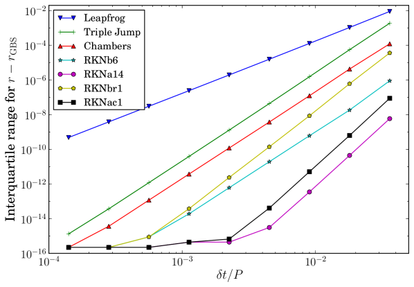
Fig. 1: Comparison of the behaviour of various methods with respect to changing step size, for gravitational two-body problem. $x$-axis the logarithm of the time step measured in orbital periods, $y$-axis is the logarithm of the interquartile range for position error. Leapfrog (down-triangles) is the standard second order Störmer-Verlet scheme, Triple jump (pluses) is the fourth order scheme of Yoshida [21], Chambers (up-triangles) is the complex third order scheme of Chambers [11],RKNb6 (stars) and RKNa14 (circles) are optimized fourth and sixth order methods by Blanes & Moan [7, 8], RKNbr1 (pentagons) and RKNac1 (squares) are two of the methods presented in this work.

The comparison indicates that, for this problem, method of Chambers [11] shows fourth order and method AC1 shows sixth order behaviour, even though they are formally third and fifth order, respectively. Analogous results were obtained by Chambers [11] for similar problems. It is interesting to see that the optimized 4th order method RKNb6 [8] outperforms a method of higher order, RKNbr1, down to machine accuracy level.

To make a more comprehensive and meaningful test, we also developed integrators for the gravitational $N$-body problem, based on various methods. We simulated the evolution of a Plummer sphere with 400 equal mass particles (see ref. [1] for a procedure for constructing a Plummer sphere). We followed the same procedure to estimate the errors and calculated the interquartile range for various methods and stepsizes. The dependence of errors on step size is given in figure 2.

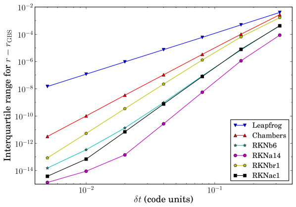
Fig. 2: Comparison of the behaviour of various methods with respect to changing step size, for gravitational 400-body problem. $x$-axis the logarithm of the time step in code units, $y$-axis is the logarithm of the interquartile range for position error. The symbols correspond to the same methods as figure 1, except Triple Jump is omitted, since it nearly coincides with Chambers for this problem.

Since complex arithmetic requires more operations than real arithmetic, we also made a comparison of CPU times for various methods. It was not possible to calculate CPU times for two-body or 400-body problems accurately, since each step took too little time. Consequently, we setup a system of 10000 particles and integrated over a few steps. While calculating the CPU time, we subtracted off the time spent for the last substep for an integration step, since all the schemes we consider have the so called first-same-as-last property. For example, in RKNA schemes (equation 13) $e^{\alpha_{1}\tau\mathbb{T}}$ substep can be combined with $e^{\alpha_{6}\tau\mathbb{T}}$ substep of the next step. We present the CPU times per step for various methods in table 4.

Table 4: CPU times spent at each step for various methods. Values are normalized to Leapfrog method’s CPU time.

Leapfrog	1
Chambers	12
Triple Jump	3
RKNb6	6
RKNa14	14
RKNbr1	5
RKNac1	28

The data here show that the integration time is proportional to the number of stages and using complex arithmetic increases the computation cost by about a factor of 6. This last factor surely depends on the problem, the implementation and the compiler. We present the error vs. CPU time, based on these findings in figure 3.

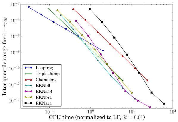
Fig. 3: CPU time spent vs. error for various methods applied to gravitational 400-body problem. $x$-axis the logarithm of the CPU time, normalized to time spent for Leapfrog method at time step $\delta t=0.01$, $y$-axis is the logarithm of the interquartile range for position error. The symbols correspond to the same methods as figure 1.

6 Discussion

In this work we constructed fifth order RKN methods with complex coefficients. Some of the methods we found have much smaller timesteps than the previously known methods, leading to smaller leading order errors. In addition, many of them have positive real coefficients, making them suitable for problems where negative real timesteps are not acceptable [12, 3, 13]. Similar methods, satisfying this requirement, were also developed by Bandrauk et al. [2]. Other high order methods with complex coefficients with small positive real parts were developed and analyzed by Hansen & Ostermann [16] and Castella et al. [10]; however these authors did not specifically study the RKN case, which allows considerable simplification for high order schemes.

For problems where complex arithmetic and/or positive real parts of the coefficients is a necessity, we expect these methods to be already competitive with lower order methods. However, the results of Blanes & Moan [8] and Sofroniou & Spaletta [20] suggest that there is room for improvement by increasing the number of stages. We consider finding fully optimized methods with more stages beyond the scope of this paper; such an effort would require developing new software and would need spending considerable computational power. However, the methods found here can be improved by readily available tools. The idea is to turn a 5-stage method into a 6-stage one by adding an additional stage.

$$e^{\alpha_{6}\tau\mathbb{T}}e^{\beta_{5}\tau\mathbb{V}}e^{\alpha_{5}\tau\mathbb{T}}\ldots e^{\beta_{1}\tau\mathbb{V}}e^{\alpha_{1}\tau\mathbb{T}}\rightarrow\\ e^{\beta^{\prime}_{7}\tau\mathbb{V}}e^{\alpha_{6}\tau\mathbb{T}}e^{\beta^{\prime}_{6}\tau\mathbb{V}}\ldots e^{\alpha_{1}\tau\mathbb{T}}e^{\beta^{\prime}_{1}\tau\mathbb{V}}\,,$$ (17)

and set $\beta^{\prime}_{7}=\beta^{\prime}_{1}=0$. We can then start in the vicinity of this solution and use MAPLE’s minimization routines. Starting from solution AC1 in table 2, we obtained the following skew-symmetric method:

$$\begin{split}\alpha_{1}&=.101907705405177865+i.130701756906677735\,,\\ \alpha_{2}&=.218628781976265590+i.0126440811480678494\,,\\ \alpha_{3}&=.179463512618556560-i.148112326926992222\,,\\ \beta^{\prime}_{1}&=.0489489561074426954+i.0669384556781967844\,,\\ \beta^{\prime}_{2}&=.166479171860817010+i.0764027877516731402\,,\\ \beta^{\prime}_{3}&=.192297943665939275-i.0835834606213808479\,,\\ \beta^{\prime}_{4}&=.184547856731601789\,.\end{split}$$ (18)

This method has an error $\left(\sum_{i}|X_{i}|^{2}\right)^{1/2}=2.6\times 10^{-7}$, about two orders of magnitude smaller than the other methods (see table 3).

Since we minimized the (imaginary) sixth order error terms, this optimization does not benefit the solutions of gravitational $N$-body problem. A possible venue for exploration is to increase the number of stages and minimize the (real part of) seventh order errors by using the extra variables. For this investigation, using a Lyndon basis would be more preferable, since the BCH expansion has much fewer terms in this basis [9] and the consequences of the simplification $[\mathbb{V},[\mathbb{V},[\mathbb{T},\mathbb{V}]]]=0$ is more straightforward. Here, we used a Philip Hall basis, since this allowed us to check our algebra by the “Lie Tools Package” of Miguel Torres-Torriti.

The source code of the MAPLE, Python and C programs used in this work are freely available online: https://github/atakan/Complex_Coeff_RKN

References

- [1] S. J. Aarseth, M. Henon, and R. Wielen, A comparison of numerical methods for the study of star cluster dynamics, Astronom. and Astrophys., 37 (1974), pp. 183–187.
- [2] André D. Bandrauk, Effat Dehghanian, and Huizhong Lu, Complex integration steps in decomposition of quantum exponential evolution operators, Chem. Phys. Lett., 419 (2006), pp. 346 – 350.
- [3] André D. Bandrauk and Hai Shen, Improved exponential split operator method for solving the time-dependent schrödinger equation, Chem. Phys. Lett., 176 (1991), pp. 428 – 432.
- [4] Sergio Blanes and Fernando Casas, On the convergence and optimization of the Baker-Campbell-Hausdorff formula, Linear Algebra and Appl., 378 (2004), pp. 135 – 158.
- [5] S. Blanes, F. Casas, and A. Murua, Splitting and composition methods in the numerical integration of differential equations, Bol. Soc. Esp. Mat. Apl., 45 (2008), pp. 87–143.
- [6] S. Blanes, F. Casas, and A. Murua, Splitting methods with complex coefficients, Bol. Soc. Esp. Mat. Apl., (2010), pp. 47–61. arXiv:1001.1549.
- [7] S. Blanes and P. C. Moan, Splitting methods for non-autonomous differential equations, J. Comput. Phys., 170 (2001), pp. 205–230.
- [8] , Practical symplectic partitioned Runge–Kutta and Runge–Kutta–Nyström methods, J. Comput. Appl. Math., 142 (2002), pp. 313–330.
- [9] F. Casas and A. Murua, An efficient algorithm for computing the Baker-Campbell-Hausdorff series and some of its applications, J. Math. Phys., 50 (2009), p. 033513.
- [10] F. Castella, P. Chartier, S. Descombes, and G. Vilmart, Splitting methods with complex times for parabolic equations, BIT, 49 (2009), pp. 487–508.
- [11] J. E. Chambers, Symplectic Integrators with Complex Time Steps, Astronom. J., 126 (2003), pp. 1119–1126.
- [12] Siu A. Chin, Quadratic diffusion monte carlo algorithms for solving atomic many-body problems, Phys. Rev. A, 42 (1990), pp. 6991–7005.
- [13] Siu A. Chin, Symplectic integrators from composite operator factorizations, Phys. Lett. A, 226 (1997), pp. 344 – 348.
- [14] E. Hairer, C. Lubich, and G. Wanner, Geometric Numerical Integration, Springer-Verlag, Berlin, 2006.
- [15] E. Hairer, S. P. Nørsett, and G. Wanner, Solving Ordinary Differential Equations: vol I, Springer-Verlag, Berlin, 1993.
- [16] Eskil Hansen and Alexander Ostermann, High order splitting methods for analytic semigroups exist, BIT, 49 (2009), pp. 527–542.
- [17] H. F. Levison and M. J. Duncan, Symplectically Integrating Close Encounters with the Sun, Astron. J., 120 (2000), pp. 2117–2123.
- [18] Daniel I. Okunbor and Robert D. Skeel, Explicit canonical methods for Hamiltonian systems, Math. Comp., (1992), pp. 439–455.
- [19] , Canonical runge–kutta–nyström methods of orders five and six, J. Comput. Appl. Math., 51 (1994), pp. 375 – 382.
- [20] M. Sofroniou and G. Spaletta, Derivation of Symmetric Composition Constants for Symmetric Integrators, Optim. Methods Softw., 20 (2005), p. 597.
- [21] H. Yoshida, Recent Progress in the Theory and Application of Symplectic Integrators, Celestial Mech. Dynam. Astronom., 56 (1993), pp. 27–43.
- [22] Wen-Jie Zhu and Meng-Zhao Qin, Order conditions of two kinds of canonical difference schemes, Comput. Math. Appl., 25 (1993), pp. 61 – 74.