Optimal control strategies for tuberculosis treatment: a case study in Angola

Abstract.

We apply optimal control theory to a tuberculosis model given by a system of ordinary differential equations. Optimal control strategies are proposed to minimize the cost of interventions. Numerical simulations are given using data from Angola.

Cristiana J. Silva and Delfim F. M. Torres

Center for Research and Development in Mathematics and Applications

Department of Mathematics, University of Aveiro, 3810-193 Aveiro, Portugal

To Professor Helmut Maurer on the occasion of his 65th birthday.

1. Introduction

Angola has one of the world’s fastest growing economies. It is a very rich country in terms of natural resources, with oil, diamonds and hydroelectric power, and a very fertile agricultural land. However, Angola remains a third world country with about one third of its population still depending on subsistence agriculture [30]. In 2009, the life expectancy at birth was 52 years, population median age was 17, 45% of the population was under age 15 and only 4% over 60 years, and the total fertility rate per woman was 5.6. Angola’s total population was 10 million in 1990 and it is approximately double that figure today. According to the Global Health Observatory Data Repository of the World Health Organization (WHO), in 2010 the infant mortality rate (probability of dying between birth and age 1) was 98 per 1,000 live births; and the under-five mortality rate (probability of dying by age 5) was 161 per 1,000 live births, which corresponds to 121,000 deaths per year.

Tuberculosis (TB) is the leading cause of death among individuals infected with the human immunodeficiency virus (HIV) and the rates of co-infection exceed 1,000 per 100,000 of total population in some countries in sub-Saharan Africa [3]. Between 1990 and 2005, TB incidence rates tripled in African countries with high HIV prevalence [24]. Recent data from Luanda Sanatorium Hospital makes it clear that TB is one of the leading causes of death in Angola [25]. In 2010 alone, there were approximately 58,000 new TB cases in Angola. The country established a National Program for the Control of Tuberculosis in 1981. However, the civil war destroyed 70% of Angola’s health facilities, leaving a substantial proportion of the population vulnerable to TB. In 2007 the Ministry of Health confirmed that the national program was implemented in only 8.6% of health units. Moreover, the internal transport and distribution networks for drugs are unreliable and 40% of clinics have experienced stockouts in TB drugs [31]. According to WHO’s Global Tuberculosis Control Report of 2010, the figures of TB in Angola are as follows: the induced mortality rate per 100,000 decreased from 42 in 1990 to 30 in 2009; the incidence rate (including HIV) increased from 205 in 1990 to 298 in 2009; the new and relapse notification rate increased from 96 in 1990 to 223 in 2009; the number of smear-positive cases increased from 3,804 in 2005 to 22,488 in 2009; the number of extra-pulmonary TB cases increased from 266 in 1995 to 3,780 in 2010; the relapse rate increased from 134 in 1995 to 2,444 in 2010; and the total number of retreated individuals increased from 134 in 1995 to 7,776 in 2010. Treatment success rates vary between 68% in 2002 and 74% in 2005, and are still within that range today, well below WHO’s target of 85% [31, 32]. The multidrug-resistant TB (resistant to, at least, isoniazid and rifampicin) was about 2% of all new cases in 2009.

TB remains a major health problem worldwide. In 2011, the regional director of WHO for Africa stated that despite the fact that member states have almost universally adopted a strategy to stop tuberculosis, the implementation of this strategy has been ineffective. Co-infections TB/HIV and TB multi-resistance to drugs are some of the reasons for the difficulty in controlling TB [22]. Most cases of TB are caused by the Mycobacterium tuberculosis, which is usually transmitted via airborne infection from someone who has active TB. Approximately 10% of infected people with Mycobacterium tuberculosis develop active TB disease, that is, approximately 90% of infected people remain latent. Latent infected TB people are asymptomatic and do not transmit TB, but may progress to active TB through endogenous reactivation or exogenous reinfection [16, 17]. The anti-TB drugs developed since 1940 have helped to reduce the mortality rates significantly: in clinical cases, cure rates of 90% have been documented and in 2009 Angola’s treatment cure rate was about 72% [21]. Three types of TB treatment are available: vaccination to prevent infection; treatment to cure active TB; and treatment of latent TB to prevent endogenous reactivation [5].

Optimal control is a branch of mathematics that involves finding optimal ways of controlling a dynamic system [1, 4, 13, 19]. While the usefulness of optimal control theory in epidemiology is nowadays well recognized [2, 9, 10, 11, 14, 15], results pertaining to tuberculosis are a rarity [7], and specific studies for the situation of Angola nonexistent. Our aim in this paper is thus to use real data from Angola to study optimal strategies for the minimization of the number of active TB infectious and persistent latent individuals, taking into account the cost of the measures for the treatment of these individuals.

The treatment of active infectious individuals can take different amounts of time [8]. Here we consider treatments with a duration of 6 months. With these treatments one of the barriers to their success is that the patients often do not complete them. Since after two months patients no longer have symptoms of the disease and feel healed, many of them stop taking the medicines. When the treatment plan is not completed, the patients are not cured and reactivation can occur and/or the patients may develop resistent TB. The lack of support from family may cause some patients to abandon treatment. Statistics from Luanda Sanatorium Hospital show that 15 of the 270 TB patients abandoned the hospital during 2010. A possible strategy to ensure patients complete the treatment involves supervision and patient support. In fact, this is one the measures proposed by WHO’s Direct Observation Therapy (DOT) [20]. One example of treatment supervision consists of recording each dose of anti-TB drugs on the patient treatment card [20]. These measures are, however, very expensive, since the patients must stay longer in the hospital or specialized people must be paid to supervise patients until they finish their treatment. On the other hand, it is recognized that the treatment of latent TB individuals reduces the chances of reactivation, even though it is still unknown how treatment influences reinfection [5].

In Section 2 we consider a mathematical model for TB from [5], which considers reinfection and post-exposure interventions. We alter this model by adding two control functions: the first control $u_{1}$ is associated with preventive measures that help active infected patients to complete the treatment; the second control $u_{2}$ governs the fraction of persistent latent individuals that is put under treatment. Our aim is stated in precise terms in Section 3: to study how the two control measures can reduce the number of infected and persistent latent individuals, taking into account the cost associated with their implementation (optimal control problem (1)–(3)). Our conclusion is that a successful implementation of these measures can prevent the increase of new and reinfected TB cases. In Section 4 we present numerical simulations for three different strategies and the corresponding optimal control solutions are discussed. We end the paper with some conclusions in Section 5.

2. TB model with controls

We study the mathematical model from [5], where reinfection and post-exposure interventions for tuberculosis are considered. To this model we add two control functions $u_{1}(\cdot)$ and $u_{2}(\cdot)$ and two real positive model constants $\epsilon_{1}$ and $\epsilon_{2}$. The resulting model is given by the following system of nonlinear ordinary differential equations:

$$\left\{\begin{aligned} \dot{S}(t)&=\mu N-\frac{\beta}{N}I(t)S(t)-\mu S(t)\\ \dot{L_{1}}(t)&=\frac{\beta}{N}I(t)\left(S(t)+\sigma L_{2}(t)+\sigma_{R}R(t)\right)-\left(\delta+\tau_{1}+\mu\right)L_{1}(t)\\ \dot{I}(t)&=\phi\delta L_{1}(t)+\omega L_{2}(t)+\omega_{R}R(t)-(\tau_{0}+\epsilon_{1}u_{1}(t)+\mu)I(t)\\ \dot{L_{2}}(t)&=(1-\phi)\delta L_{1}(t)-\sigma\frac{\beta}{N}I(t)L_{2}(t)-(\omega+\epsilon_{2}u_{2}(t)+\tau_{2}+\mu)L_{2}(t)\\ \dot{R}(t)&=(\tau_{0}+\epsilon_{1}u_{1}(t))I(t)+\tau_{1}L_{1}(t)+(\tau_{2}+\epsilon_{2}u_{2}(t))L_{2}(t)-\sigma_{R}\frac{\beta}{N}I(t)R(t)\\ &\quad\quad\quad-(\omega_{R}+\mu)R(t)\,.\end{aligned}\right.$$ (1)

The population is divided into five categories (i.e., control system (1) has five state variables):

• susceptible ($S$);

• early latent ($L_{1}$), i.e., individuals recently infected (less than two years) but not infectious;

• infected ($I$), i.e., individuals who have active TB and are infectious;

• persistent latent ($L_{2}$), i.e., individuals who were infected and remain latent;

• and recovered ($R$), i.e., individuals who were previously infected and have been treated.

The control $u_{1}$ represents the effort in preventing the failure of treatment in active TB infectious individuals $I$, e.g., supervising the patients, helping them to take the TB medications regularly and to complete the TB treatment. The control $u_{2}$ governs the fraction of persistent latent individuals $L_{2}$ that is put under treatment. The parameters $\epsilon_{i}\in(0,1)$, $i=1,2$, measure the effectiveness of the controls $u_{i}$, $i=1,2$, respectively, i.e., these parameters measure the efficacy of treatment interventions for active and persistent latent TB individuals, respectively. We assume that the total population, $N$, with $N=S(t)+L_{1}(t)+I(t)+L_{2}(t)+R(t)$, is constant in time. In other words, we assume that the birth and death rates are equal. By virtue of this assumption, we can reduce the control system (1) from five to four state variables. However, in this paper we prefer to keep the TB model in form (1), using relation $S(t)+L_{1}(t)+I(t)+L_{2}(t)+R(t)=N$ as a test to check the numerical results.

Following WHO’s Global Health Observatory for Angola in 2009 [23], we consider $\mu=1/52\,yr^{-1}$, which corresponds to a life expectancy at birth of 52 years. This and other values of the parameters are given in Table 1. Moreover, following [5], we assume that there are no disease-related deaths, and that at birth all individuals are equally susceptible and become different as they experience infection and respective therapy. The proportion of the population in each category changes according to the system (1).

Two different values for the initial conditions $S(0)$, $L_{1}(0)$, $I(0)$, $L_{2}(0)$ and $R(0)$ are considered (see Table 2):

• Case 1, initial values are borrowed from [7];

• Case 2, initial values are based on the data from Luanda’s Sanatorium Hospital during September 2010 [25].

The values of the rates $\delta$, $\phi$, $\omega$, $\omega_{R}$, $\sigma$ and $\tau_{0}$ are taken from [5] and the references cited therein (see Table 1 for the values of all the parameters). The parameter $\delta$ denotes the rate at which individuals leave the $L_{1}$ category; $\phi$ is the proportion of individuals going to category $I$; $\omega$ is the rate of endogenous reactivation for persistent latent infections (untreated latent infections); and $\omega_{R}$ is the rate of endogenous reactivation for treated individuals (for those who have undergone a therapeutic intervention). The parameter $\sigma$ is a factor that measures the reduction in the risk of infection, as a result of acquired immunity to a previous infection, for persistent latent individuals, i.e., this factor affects the rate of exogenous reinfection of untreated individuals; while $\sigma_{R}$ represents the same parameter factor but for treated patients. In our simulations we consider the case where the susceptibility to reinfection of treated individuals equals that of latents: $\sigma_{R}=\sigma$. The parameter $\tau_{0}$ is the rate of recovery under treatment of active TB (assuming an average infectiousness duration of six months). The parameters $\tau_{1}$ and $\tau_{2}$ apply to latent individuals $L_{1}$ and $L_{2}$, respectively, and are the rates at which chemotherapy or a post-exposure vacine is applied. In [5], different values for these rates are considered: the case where no treatment of latent infections occur ($\tau_{1}=\tau_{2}=0$); the case where there is an immediate treatment of persistent latent infections ($\tau_{2}\to\infty$); and the case where there is a moderate treatment of persistent latent infections ($\tau_{2}\in[0.1,1]$). The first and second cases are not interesting from the optimal control point of view. In our paper we consider, without loss of generality, that the rate of recovery of early latent individuals under post-exposure interventions is equal to the rate of recovery under treatment of active TB, $\tau_{1}=2\,yr^{-1}$, and greater than the rate of recovery of persistent latent individuals under post-exposure interventions, $\tau_{2}=1\,yr^{-1}$. It is assumed that the rate of infection for susceptible individuals is proportional to the number of infectious individuals and the constant of proportionality is $\beta$, which is the transmission coefficient.

From the epidemiologistic point of view, an important quantity is given by the basic reproduction number $R_{0}$. This is the expected number of secondary cases produced in a complete susceptible population, by a typical infected individual during his/her entire period of infectiousness [15]. In the absence of controls ($u_{1}=u_{2}\equiv 0$), it is known (see [5]) that the basic reproduction number for system (1) is proportional to the transmission coefficient $\beta$:

$$R_{0}=\beta\frac{\delta(\omega+\phi\mu)(\omega_{R}+\mu)}{\mu(\omega_{R}+\tau_{0}+\mu)(\delta+\mu)(\omega+\mu)}.$$

The endemic threshold is given at $R_{0}=1$ and indicates the minimal transmission potential that sustains endemic disease, i.e., when $R_{0}<1$ the disease will die out and for $R_{0}>1$ the disease may become endemic. We can prove that variations of the parameter $\beta$ are associated with different values for the optimal control $u_{1}$ but do not interfere significantly with the optimal control $u_{2}$. Moreover, as expected, as $\beta$ decreases the fraction of latent and infected individuals also decreases. Here we consider $\beta=100$, which corresponds to the endemic case ($R_{0}=2.96>1$). The measures of control efficacy are fixed to the values $\epsilon_{i}=1/2$, $i=1,2$. Because the risk of developing disease after infection is much higher in the first five years following infection, and declines exponentially after that [18, Sec. 5.5], we take the total simulation time duration as $T=5$ years.

3. The optimal control problem

Consider the state system (1) of ordinary differential equations in $\mathbb{R}^{5}$ with the set of admissible control functions given by

$$\Omega=\{(u_{1}(\cdot),u_{2}(\cdot))\in(L^{\infty}(0,T))^{2}\,|\,0\leq u_{1}(t),u_{2}(t)\leq 1,\,\forall\,t\in[0,T]\,\}.$$

The objective functional is given by

$$J(u_{1}(\cdot),u_{2}(\cdot))=\int_{0}^{T}\left[I(t)+L_{2}(t)+\tfrac{1}{2}W_{1}u_{1}^{2}(t)+\tfrac{1}{2}W_{2}u_{2}^{2}(t)\right]dt\,,$$ (2)

where the constants $W_{1}$ and $W_{2}$ are a measure of the relative cost of the interventions associated with the controls $u_{1}$ and $u_{2}$, respectively. In our numerical simulations we consider the weight $W_{1}$ associated with the control $u_{1}$ to be greater than the weight $W_{2}$ associated with $u_{2}$: $W_{1}=500$ and $W_{2}=50$. The reason for this is that the cost associated with $u_{1}$ includes the cost of holding active infected patients $I$ in the hospital or paying professionals to supervise them, ensuring that they finish their treatment, which is costly to implement. In Section 4.4 we compare this situation to the one when the weights take the same values: $W_{1}=W_{2}=50$. We consider the optimal control problem of determining $\left(S^{*}(\cdot),L_{1}^{*}(\cdot),I^{*}(\cdot),L_{2}^{*}(\cdot),R^{*}(\cdot)\right)$, associated with an admissible control pair $\left(u_{1}^{*}(\cdot),u_{2}^{*}(\cdot)\right)\in\Omega$ on the time interval $[0,T]$, satisfying (1), the initial conditions $S(0)$, $L_{1}(0)$, $I(0)$, $L_{2}(0)$ and $R(0)$ (see Table 2), and minimizing the cost functional (2), i.e.,

$$J(u_{1}^{*}(\cdot),u_{2}^{*}(\cdot))=\min_{\Omega}J(u_{1}(\cdot),u_{2}(\cdot))\,.$$ (3)

Theorem 3.1.

The problem (1), (3) with fixed initial conditions $S(0)$, $L_{1}(0)$, $I(0)$, $L_{2}(0)$ and $R(0)$, and fixed final time $T$, admits a unique optimal solution $\left(S^{*}(\cdot),L_{1}^{*}(\cdot),I^{*}(\cdot),L_{2}^{*}(\cdot),R^{*}(\cdot)\right)$ associated with an optimal control pair $\left(u_{1}^{*}(\cdot),u_{2}^{*}(\cdot)\right)$ on $[0,T]$. Moreover, there exist adjoint functions, $\lambda_{1}^{*}(\cdot)$, $\lambda_{2}^{*}(\cdot)$, $\lambda_{3}^{*}(\cdot)$, $\lambda_{4}^{*}(\cdot)$ and $\lambda_{5}^{*}(\cdot)$, such that

$$\left\{\begin{split}\dot{\lambda^{*}_{1}}(t)&=\lambda^{*}_{1}(t)\left(\frac{\beta}{N}I^{*}(t)+\mu\right)-\lambda^{*}_{2}(t)\frac{\beta}{N}I^{*}(t)\\ \dot{\lambda^{*}_{2}}(t)&=\lambda^{*}_{2}(t)(\delta+\tau_{1}+\mu)-\lambda^{*}_{3}(t)\phi\delta-\lambda^{*}_{4}(t)(1-\phi)\delta-\lambda^{*}_{5}(t)\tau_{1}\\ \dot{\lambda^{*}_{3}}(t)&=-1+\lambda^{*}_{1}(t)\frac{\beta}{N}S^{*}(t)-\lambda^{*}_{2}(t)\frac{\beta}{N}(S^{*}(t)+\sigma L_{2}^{*}(t)+\sigma_{R}R^{*}(t))\\ +\lambda^{*}_{3}&(t)(\tau_{0}+\epsilon_{1}u_{1}^{*}(t)+\mu)+\lambda^{*}_{4}(t)\sigma\frac{\beta}{N}L_{2}^{*}(t)-\lambda^{*}_{5}(t)\left(\tau_{0}+\epsilon_{1}u^{*}_{1}(t)-\sigma_{R}\frac{\beta}{N}R^{*}(t)\right)\\ \dot{\lambda^{*}_{4}}(t)&=-1-\lambda^{*}_{2}(t)\frac{\beta}{N}I^{*}(t)\sigma-\lambda^{*}_{3}(t)\omega+\lambda^{*}_{4}(t)\left(\sigma\frac{\beta}{N}I^{*}(t)+\omega+\epsilon_{2}u^{*}_{2}(t)+\tau_{2}+\mu\right)\\ -\lambda^{*}_{5}&(t)\left(\tau_{2}+\epsilon_{2}u^{*}_{2}(t)\right)\\ \dot{\lambda^{*}_{5}}(t)&=-\lambda^{*}_{2}(t)\sigma_{R}\frac{\beta}{N}I^{*}(t)-\lambda^{*}_{3}(t)\omega_{R}+\lambda^{*}_{5}(t)\left(\sigma_{R}\frac{\beta}{N}I^{*}(t)+\omega_{R}+\mu\right)\,,\end{split}\right.$$ (4)

with transversality conditions $\lambda^{*}_{i}(T)=0$, $i=1,\ldots,5$. Furthermore,

$$\begin{split}u_{1}^{*}(t)&=\min\left\{\max\left\{0,\frac{\epsilon_{1}I^{*}(\lambda^{*}_{3}-\lambda^{*}_{5})}{W_{1}}\right\},1\right\}\,,\\ u_{2}^{*}(t)&=\min\left\{\max\left\{0,\frac{\epsilon_{2}L^{*}_{2}(\lambda^{*}_{4}-\lambda^{*}_{5})}{W_{2}}\right\},1\right\}\,.\end{split}$$ (5)

Proof.

The existence of optimal controls $\left(u_{1}^{*}(\cdot),u_{2}^{*}(\cdot)\right)$ and associated optimal solution $\left(S^{*},L_{1}^{*},I^{*},L_{2}^{*},R^{*}\right)$ comes from the convexity of the integrand of the cost function (2) with respect to the controls $(u_{1},u_{2})$ and the Lipschitz property of the state system with respect to state variables $\left(S,L_{1},I,L_{2},R\right)$ (see, e.g., [1, 4] for existence results of optimal solutions). According to the Pontryagin Maximum Principle [13], if $(u_{1}^{*}(\cdot),u_{2}^{*}(\cdot))\in\Omega$ is optimal for the problem (1), (3) with the initial conditions given in Table 2 and fixed final time $T$, then there exists a nontrivial absolutely continuous mapping $\lambda:[0,T]\to\mathbb{R}^{5}$, $\lambda(t)=\left(\lambda_{1}(t),\lambda_{2}(t),\lambda_{3}(t),\lambda_{4}(t),\lambda_{5}(t)\right)$, called the adjoint vector, such that

$$\left\{\begin{split}\dot{S}&=\frac{\partial H}{\partial\lambda_{1}}\,,\\ \dot{L}_{1}&=\frac{\partial H}{\partial\lambda_{2}}\,,\\ \dot{I}&=\frac{\partial H}{\partial\lambda_{3}}\,,\\ \dot{L}_{2}&=\frac{\partial H}{\partial\lambda_{4}}\,,\\ \dot{R}&=\frac{\partial H}{\partial\lambda_{5}}\end{split}\right.$$

and

$$\begin{cases}\dot{\lambda}_{1}=-\frac{\partial H}{\partial S}\,,\\ \dot{\lambda}_{2}=-\frac{\partial H}{\partial L_{1}}\,,\\ \dot{\lambda}_{3}=-\frac{\partial H}{\partial I}\,,\\ \dot{\lambda}_{4}=-\frac{\partial H}{\partial L_{2}}\,,\\ \dot{\lambda}_{5}=-\frac{\partial H}{\partial R}\,,\end{cases}$$ (6)

where the Hamiltonian $H$ is defined by

$$\begin{split}H&=H(S,L_{1},I,L_{2},R,\lambda,u_{1},u_{2})\\ &=I+L_{2}+\frac{W_{1}}{2}u_{1}^{2}+\frac{W_{2}}{2}u_{2}^{2}\\ &\quad+\lambda_{1}\left(\mu N-\frac{\beta}{N}IS-\mu S\right)\\ &\quad+\lambda_{2}\left(\frac{\beta}{N}I\left(S+\sigma L_{2}+\sigma_{R}R\right)-(\delta+\tau_{1}+\mu)L_{1}\right)\\ &\quad+\lambda_{3}\left(\phi\delta L_{1}+\omega L_{2}+\omega_{R}R-(\tau_{0}+\epsilon_{1}u_{1}+\mu)I\right)\\ &\quad+\lambda_{4}\left((1-\phi)\delta L_{1}-\sigma\frac{\beta}{N}IL_{2}-(\omega+\epsilon_{2}u_{2}+\tau_{2}+\mu)L_{2}\right)\\ &\quad+\lambda_{5}\left((\tau_{0}+\epsilon_{1}u_{1})I+\tau_{1}L_{1}+\left(\tau_{2}+\epsilon_{2}u_{2}\right)L_{2}-\sigma_{R}\frac{\beta}{N}IR-(\omega_{R}+\mu)R\right)\end{split}$$

and the minimization condition

$$H\left(S^{*}(t),L_{1}^{*}(t),I^{*}(t),L_{2}^{*}(t),R^{*}(t),\lambda^{*}(t),u_{1}^{*}(t),u_{2}^{*}(t)\right)\\ =\min_{0\leq u_{1},u_{2}\leq 1}H\left(S^{*}(t),L_{1}^{*}(t),I^{*}(t),L_{2}^{*}(t),R^{*}(t),\lambda^{*}(t),u_{1},u_{2}\right)$$ (7)

holds almost everywhere on $[0,T]$. Moreover, the transversality conditions $\lambda_{i}(T)=0$, $i=1,\ldots,5$, hold. System (4) is derived from (6), and the optimal controls (5) come from the minimization condition (7). For small final time $T$, the optimal control pair given by (5) is unique due to the boundedness of the state and adjoint functions and the Lipschitz property of systems (1) and (4) (see, e.g., [7]). ∎

4. Numerical results and discussion

In this section we present different optimal control strategies for the TB model (1) under the parameter values given in Table 1. Three control strategies are explored:

• Strategy 1, which implements measures that prevent the failure of treatment in active TB individuals $I$ (control $u_{1}$ alone);

• Strategy 2, which considers treatment of persistent latent individuals $L_{2}$ with anti-TB drugs (control $u_{2}$ alone);

• Strategy 3, which implements measures for preventing treatment failure in active TB individuals and variation of the fraction of persistent latent individuals that are put under treatment (controls $u_{1}$ and $u_{2}$).

Symbol	Description	Value
$\beta$	Transmission coefficient	$100$
$\mu$	Death and birth rate	$1/52\,yr^{-1}$
$\delta$	Rate at which individuals leave $L_{1}$	$12\,yr^{-1}$
$\phi$	Proportion of individuals going to $I$	$0.05$
$\omega$	Endogenous reactivation rate for persistent latent infections	$0.0002\,yr^{-1}$
$\omega_{R}$	Endogenous reactivation rate for treated individuals	$0.00002\,yr^{-1}$
$\sigma$	Factor reducing the risk of infection as a result of acquired
	immunity to a previous infection for $L_{2}$	$0.25$
$\sigma_{R}$	Rate of exogenous reinfection of treated patients	0.25
$\tau_{0}$	Rate of recovery under treatment of active TB	$2\,yr^{-1}$
$\tau_{1}$	Rate of recovery under treatment of latent individuals $L_{1}$	$2\,yr^{-1}$
$\tau_{2}$	Rate of recovery under treatment of latent individuals $L_{2}$	$1\,yr^{-1}$
$N$	Total population	$30,000$
$T$	Total simulation duration	$5$ $yr$
$\epsilon_{1}$	Efficacy of treatment of active TB $I$	$0.5$
$\epsilon_{2}$	Efficacy of treatment of latent TB $L_{2}$	$0.5$
$W_{1}$	Weight constant of control $u_{1}$	$500$
$W_{2}$	Weight constant of control $u_{2}$	$50$

Table 1. Parameter values for the optimal control problem (1)–(3)

Different approaches were used to obtain and confirm the numerical results. One approach consisted in using IPOPT [26] and the algebraic modeling language AMPL [27]. A second approach was to use the PROPT Matlab Optimal Control Software [28]. The results coincide with the ones obtained by an iterative method that consists in solving the system of ten ODEs given by (1) and (4). For that, first one solves system (1) with a guess for the controls over the time interval $[0,T]$ using a forward fourth-order Runge–Kutta scheme and the transversality conditions $\lambda_{i}(T)=0$, $i=1,\ldots,5$. Then, system (4) is solved by a backward fourth-order Runge–Kutta scheme using the current iteration solution of (1). The controls are updated by using a convex combination of the previous controls and the values from (5). The iteration is stopped if the values of unknowns at the previous iteration are very close to the ones at the present iteration. For more details see, e.g., [7].

To begin, we study the influence of the initial values of the state variables, as given in Table 2, on the optimal solution associated with Strategy 3.

States	Case 1	Case 1	Case 2	Case 2
(initial value)	(fraction)	($\%$)	(fraction)	($\%$)
$S(0)$	$(76/120)N$	$\simeq 63.3\%$	$(16/50)N$	$32\%$
$L_{1}(0)$	$(36/120)N$	$30\%$	$(28/50)N$	$56\%$
$I(0)$	$(5/120)N$	$\simeq 4.2\%$	$(3/50)N$	$6\%$
$L_{2}(0)$	$(2/120)N$	$\simeq 1.7\%$	$(2/50)N$	$4\%$
$R(0)$	$(1/120)N$	$\simeq 0.8\%$	$(1/50)N$	$2\%$

Table 2. Initial values for the state variables of (1)

4.1. Different initial values (Case 1 and Case 2) for the state variables

Our aim is to compare the optimal solution associated with Strategy 3 (when both controls $u_{1}$ and $u_{2}$ are considered) under different initial values for the state variables: in the first case we consider the initial values of [7] (Case 1) and in the second case we consider the initial values given in an official communication from Luanda Sanatorium Hospital [25] (Case 2).

(a) Optimal Control $u_{1}^{*}$

(b) Optimal Control $u_{2}^{*}$

Figure 1. Optimal control functions in Case 1 (solid line) and Case 2 (dashed line), in a time scale in units of years, for Strategy 3

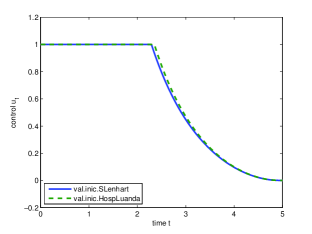
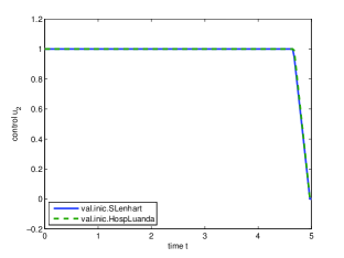
In Figure 1 we observe that the differences between the initial values considered in Cases 1 and 2 (Table 2) do not influence the optimal controls significantly.

(a) $(I^{*}+L_{2}^{*})/N$

(b) $S^{*}/N$

(c) $L_{1}^{*}/N$

(d) $R^{*}/N$

Figure 2. Optimal states in Case 1 (solid line) and Case 2 (dashed line), in a time scale in units of years, for Strategy 3

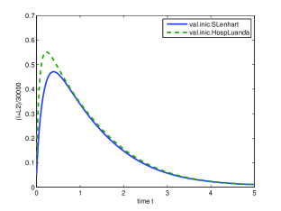
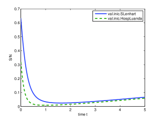
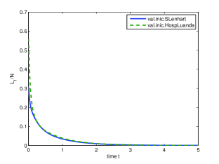
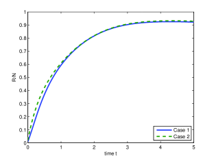
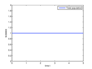
In Case 1, the initial percentage of susceptible individuals $S(0)$ is approximately twice the respective percentage in Case 2. However, with the optimal controls $\left(u_{1}^{*},u_{2}^{*}\right)$ illustrated in Figure 1, after two years this difference is substantially reduced, as we can observe in Figure 2. With respect to the initial values of early latent individuals $L_{1}(0)$, the percentage in Case 1 is 30% and in Case 2 it is 56%. Here, in both cases, the percentage of early latent individuals is reduced to approximately 10% after approximately 140 days. We observe that even if in Case 2 the initial fraction of early latent individuals is much higher than in Case 1, the optimal controls ensure a big reduction in the fraction of early latent individuals and, after no more than 5 months, the difference between the two cases no longer exists. Given these results, from now on we consider, without loss of generality, Case 1 for the initial values of the state variables. Our numerical simulations were checked using the relation $S(t)+L_{1}(t)+I(t)+L_{2}(t)+R(t)=N$. Figure 3 shows that $S(t)+L_{1}(t)+I(t)+L_{2}(t)+R(t)$ is constant along time for Strategy 3, as expected.

Figure 3. Plot of $\left(S(t)+L_{1}(t)+I(t)+L_{2}(t)+R(t)\right)/N$ versus $t$ in years for Strategy 3

4.2. Strategy 1 versus Strategy 3

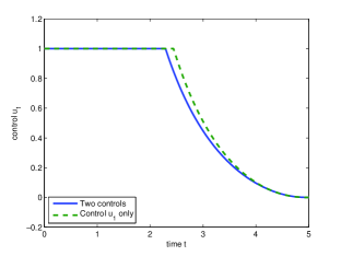
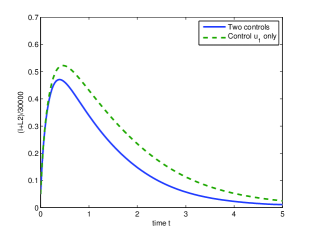
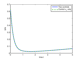
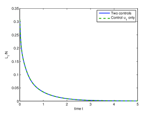
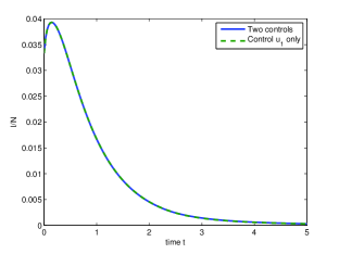
If we choose to apply only the control $u_{1}$ (Strategy 1) and compare this situation to the case where both controls $u_{1}$ and $u_{2}$ are applied (Strategy 3), we observe that the optimal control $u_{1}^{*}$ stays at the upper bound for almost the same duration in both situations (see Figure 4).

(a) Control $u_{1}^{*}$

Figure 4. The optimal control $u_{1}^{*}$ for Strategy 1 (dashed line) and Strategy 3 (solid line) in a time scale in units of years

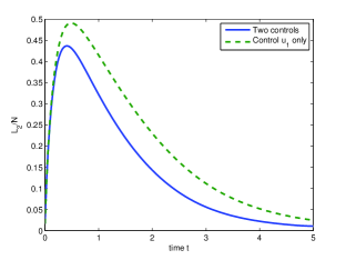
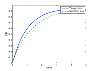
When only the control $u_{1}$ is considered, the fraction of persistent latent individuals $L_{2}$ is greater than the respective fraction associated with Strategy 3, for the entire five years (see Figure 5 A and E). This implies a higher value of the cost functional (2) associated with Strategy 1 when compared to the cost associated with Strategy 3. When one compares the change in the fraction of susceptible ($S$), early latent ($L_{1}$) and infected ($I$) individuals, no difference is observed between Strategies 1 and 3 (see Figure 5 B, C and D).

(a) $(I^{*}+L_{2}^{*})/N$

(b) $S^{*}/N$

(c) $L_{1}^{*}/N$

(d) $I^{*}/N$

(e) $L_{2}^{*}/N$

(f) $R^{*}/N$

Figure 5. Optimal states for Strategy 1 (dashed line) and Strategy 3 (solid line) in a time scale in units of years

4.3. Strategy 2 versus Strategy 3

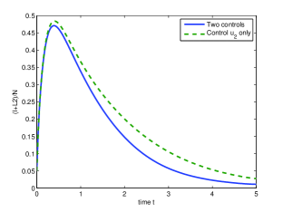
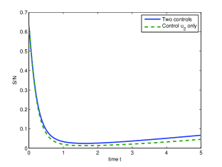
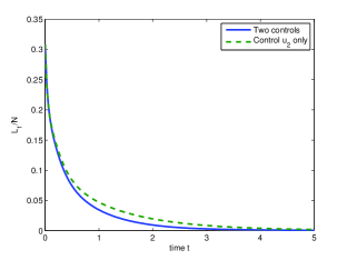
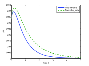
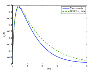
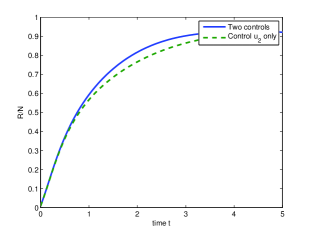
When we compare Strategy 2 (only control $u_{2}$) with Strategy 3 (both controls $u_{1}$ and $u_{2}$), we observe that the best choice is definitely to use Strategy 3. Indeed, with Strategy 3, there is a lower fraction of early and persistent latent individuals as well as infected individuals (see Figure 6 A, C, D and E). The fraction of susceptible and recovered individuals is higher when two controls are applied at the same time (see Figure 6 B and F). Similarly with Strategy 1, the value of the cost functional (2) associated with Strategy 3 is lower than that of Strategy 2.

(a) $(I^{*}+L_{2}^{*})/N$

(b) $S^{*}/N$

(c) $L_{1}^{*}/N$

(d) $I^{*}/N$

(e) $L_{2}^{*}/N$

(f) $R^{*}/N$

Figure 6. Optimal states for Strategy 2 (dashed line) and Strategy 3 (solid line) in a time scale in units of years

4.4. Changing the relative cost of interventions

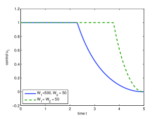
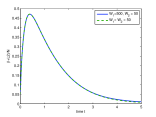
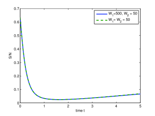
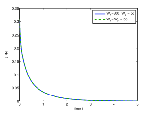
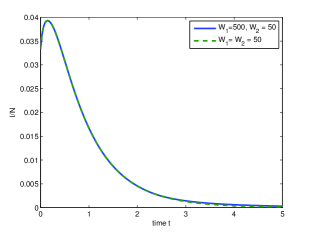
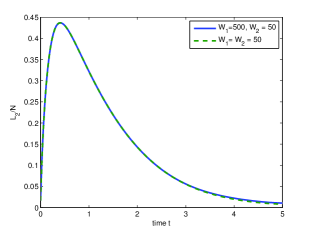
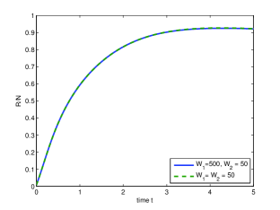
So far all the simulations were done assuming that the weight $W_{1}$ associated with the control $u_{1}$ is greater than the weight $W_{2}$ associated with $u_{2}$: $W_{1}=500$ and $W_{2}=50$ (see Table 1). We now consider the case when the weights are the same: $W_{1}=W_{2}=50$. In Figure 7 we observe that a higher weight associated with the control $u_{1}$ implies that the optimal control $u_{1}^{*}$ stays at the upper bound for a smaller duration. Surprisingly, this change in the control does not result in a change of the behavior of the state variables (see Figure 8). The results with $W_{1}=W_{2}=50$ for Strategy 1 are similar to the ones reported in Section 4.2 (including the number of days that the optimal control $u_{1}^{*}$ stays at the upper bound).

(a) Optimal control $u_{1}^{*}$

Figure 7. Optimal control $u_{1}^{*}$ for Strategy 3 in a time scale in units of years: $W_{1}=500$ and $W_{2}=50$ (solid line) versus $W_{1}=W_{2}=50$ (dashed line)

(a) $(I^{*}+L_{2}^{*})/N$

(b) $S^{*}/N$

(c) $L_{1}^{*}/N$

(d) $I^{*}/N$

(e) $L_{2}^{*}/N$

(f) $R^{*}/N$

Figure 8. Optimal states for Strategy 3 in a time scale in units of years: $W_{1}=500$ and $W_{2}=50$ (solid line) versus $W_{1}=W_{2}=50$ (dashed line)

5. Conclusion

Tuberculosis (TB) is an important health issue all over the world, particularly in many African countries. In this article we focused our attention in Angola where, since 2009, it is recognized by authorities that TB and HIV are the two most serious public health problems. Efforts to control TB in Angola have been underway since 1981, but results are still not satisfactory, and minimizing the effects caused by TB is an important challenge. Implemented measures to control these problems are having a positive effect, but the reduction rate is very slow [29].

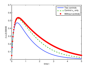
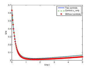
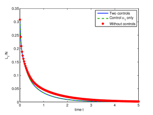
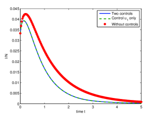
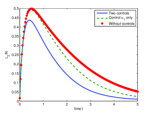
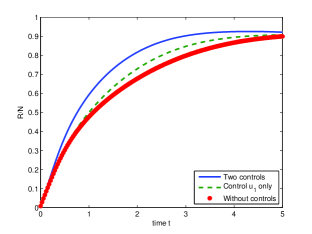
We introduced two control functions $u_{1}$ and $u_{2}$ to an existing mathematical model for TB developed in [5]. These controls are associated with measures that help to reduce the number of active infected and persistent latent TB individuals: the control $u_{1}$ represents the effort that prevents the failure of treatment in active TB infectious individuals $I$, e.g., supervising the patients, helping them to take the TB medications regularly and to complete the TB treatment; while the control $u_{2}$ governs the fraction of persistent latent individuals $L_{2}$ under treatment with anti-TB drugs. An optimal control problem was formulated and solved theoretically using the Pontryagin maximum principle. The solution to the problem was then illustrated by numerical simulations using available data from Angola. From the numerical results, one may conclude that considering only control $u_{1}$ (Strategy 1) or only control $u_{2}$ (Strategy 2) does not lead to the best results in terms of the number of active infected and persistent latent individuals. A combined strategy (Strategy 3) that involves both controls is preferable. Figure 9 shows the simulation of the system for the uncontrolled case, when $u_{1}=0$ and $u_{2}=0$, compared with the strategies here proposed. Results justify the need for intervention in tuberculosis treatment. The values of Table 3 put in evidence that the uncontrolled situation is the worst: does not only result in more infected and persistent latent individuals (1,584 individuals at the end of five years versus 334 individuals in the case Strategy 3 is applied) but also gives a higher value to the cost functional (2).

(a) $(I+L_{2})/N$

(b) $S/N$

(c) $L_{1}/N$

(d) $I/N$

(e) $L_{2}/N$

(f) $R/N$

Figure 9. State variables with and without controls in a time scale in units of years

	Strategy 1	Strategy 2	Strategy 3	Without controls
$I(5)+L_{2}(5)$	$\simeq 751$	$\simeq 831$	$\simeq 334$	$\simeq 1,584$
Cost: functional (2)	$\simeq 32,511.2$	$\simeq 28,585.9$	$\simeq 24,133.1$	$\simeq 37,760.3$

Table 3. Comparison of Strategies 1, 2, 3 with the uncontrolled case, i.e., when $u_{1}=u_{2}=0$

References

- [1] (MR0688142) L. Cesari, Optimization—Theory and Applications. Problems with Ordinary Differential Equations, Applications of Mathematics 17, Springer-Verlag, New York, 1983.
- [2] (MR2597086) A. d’Onofrio, U. Ledzewicz, H. Maurer and H. Schättler, On optimal delivery of combination therapy for tumors, Math. Biosci., 222, N. 1 (2009) 13–26.
- [3] C. Dye, S. Scheele, P. Dolin, V. Pathania and M. C. Raviglione, Global burden of tuberculosis. Estimated incidence, prevalence, and mortality by country, Journal of the American Medical Association, 282 (1999) 677–686.
- [4] (MR0454768) W.H. Fleming and R.W. Rishel, Deterministic and Stochastic Optimal Control, Applications of Mathematics, No. 1. Springer-Verlag, Berlin-New York, 1975.
- [5] M. G. M. Gomes, P. Rodrigues, F. M. Hilker, N. B. Mantilla-Beniers, M. Muehlen, A. C. Paulo and G. F. Medley, Implications of partial immunity on the prospects for tuberculosis control by post-exposure interventions, Journal of Theoretical Biology, 248 (2007) 608–617.
- [6] L.S. Jennings, M.E. Fisher, K.L. Teo and C.J. Goh, MISER3 Optimal Control Software: Theory and User Manual, Version 3.3, Department of Mathematics, The University of Western Australia, Nedlands, Australia, 2004.
- [7] (MR1921233) E. Jung, S. Lenhart and Z. Feng, Optimal control of treatments in a two-strain tuberculosis model, Discrete and Continuous Dynamical Systems - Series B, 2, N. 4 (2002) 473–482.
- [8] M. E. Kruk, N. R. Schwalbe and C. A. Aguiar, Timing of default from tuberculosis treatment: a systematic review, Tropical Medicine and International Health, 13, N. 5 (2008) 703–712.
- [9] (MR2657555) U. Ledzewicz, J. Marriott, H. Maurer and H. Schättler, Realizable protocols for optimal administration of drugs in mathematical models for anti-angiogenic treatment, Math. Med. Biol. 27, N. 2 (2010) 157–179.
- [10] (MR2793485) U. Ledzewicz, H. Maurer and H. Schättler, Optimal and suboptimal protocols for a mathematical model for tumor anti-angiogenesis in combination with chemotherapy, Math. Biosci. Eng. 8, N. 2 (2011) 307–323.
- [11] (MR2316829) S. Lenhart, J. T. Workman, Optimal control applied to biological models, Chapman & Hall/CRC, Boca Raton, FL, 2007.
- [12] (MR2527217) R. C. Loxton, K. L. Teo and V. Rehbock, Optimal control problems with multiple characteristic time points in the objective and constraints, Automatica J. IFAC 44, N. 11 (2008) 2923–2929.
- [13] (MR0166037) L. Pontryagin, V. Boltyanskii, R. Gramkrelidze and E. Mischenko, The Mathematical Theory of Optimal Processes, Wiley Interscience, 1962.
- [14] (MR2719552) H. S. Rodrigues, M. T. T. Monteiro and D. F. M. Torres, Dynamics of dengue epidemics when using optimal control, Math. Comput. Modelling, 52, N. 9-10 (2010) 1667–1673. arXiv:1006.4392
- [15] H. S. Rodrigues, M. T. T. Monteiro, D. F. M. Torres and A. Zinober, Dengue disease, basic reproduction number and control, Int. J. Comput. Math., 89, N. 3 (2012) 334–346. arXiv:1103.1923
- [16] P.M. Small and P.I. Fujiwara, Management of tuberculosis in the United States, N. Engl. J. Med., 345 (2001) 189–200.
- [17] K. Styblo, State of art: epidemiology of tuberculosis, Bull. Int. Union Tuberc., 53 (1978) 141–152.
- [18] K. Styblo, Selected papers, Epidemiology of tuberculosis, Royal Netherlands Tuberculosis Association, 24 (Sec. 5.5.) (1991).
- [19] (MR1153024) K.L. Teo, C.J. Goh and K.H. Wong, A unified computational approach to optimal control problems, Pitman Monographs and Surveys in Pure and Applied Mathematics, 55, Longman Sci. Tech., Harlow, 1991.
- [20] WHO, Treatment of tuberculosis guidelines, Fourth edition, WHO, Geneva, 2010. http://www.who.int/tb/publications/tb_treatmentguidelines/en/index.html
- [21] WHO, Global Tuberculosis Control, WHO Report 2011, Geneva, 2011. http://www.who.int/tb/publications/global_report/en/index.html
- [22] http://allafrica.com/stories/201103240476.html
- [23] http://apps.who.int/ghodata/?theme=country
- [24] http://www.avert.org/tuberculosis.htm
- [25] http://www.minsa.gov.ao/VerNoticia.aspx?id=10499
- [26] https://projects.coin-or.org/Ipopt
- [27] http://www.ampl.com
- [28] http://tomdyn.com
- [29] http://www.minsa.gov.ao/VerNoticia.aspx?id=8797
- [30] http://www.tradingeconomics.com/angola/tuberculosis-case-detection-rate-all-forms-wb-data.html
- [31] http://www.usaid.gov/our_work/global_health/id/tuberculosis/countries/africa/angola_profile.html
- [32] http://www.who.int/en/