Numerical computations and mathematical modelling with infinite and infinitesimal numbers

Abstract

Traditional computers work with finite numbers. Situations where the usage of infinite or infinitesimal quantities is required are studied mainly theoretically. In this paper, a recently introduced computational methodology (that is not related to the non-standard analysis) is used to work with finite, infinite, and infinitesimal numbers numerically. This can be done on a new kind of a computer – the Infinity Computer – able to work with all these types of numbers. The new computational tools both give possibilities to execute computations of a new type and open new horizons for creating new mathematical models where a computational usage of infinite and/or infinitesimal numbers can be useful. A number of numerical examples showing the potential of the new approach and dealing with divergent series, limits, probability theory, linear algebra, and calculation of volumes of objects consisting of parts of different dimensions are given.

Key Words: Numerical computations, infinite and infinitesimal numbers, the Infinity Computer.

1 Introduction

The point of view on infinity accepted nowadays takes its origins from the famous ideas of Georg Cantor (see [2]). Different generalizations of the traditional arithmetic for finite numbers to the case of infinite and infinitesimal numbers have been proposed in literature (see, e.g., [1, 2, 3, 6, 7] and references given therein). However, these generalizations are quite different with respect to the finite arithmetic we are used to deal with. Moreover, very often they leave undetermined many operations where infinite numbers take part (e.g., $\infty-\infty$, $\frac{\infty}{\infty}$, etc.) or use representation of infinite numbers based on infinite sequences of finite numbers.

In spite of these crucial difficulties and due to the enormous importance of the concept of infinite and infinitesimal in Science, people try to introduce these notions in their work with computers. Thus, the IEEE Standard for Binary Floating-Point Arithmetic (IEEE 754) being the most widely-used standard for floating-point computation defines formats for representing special values for positive and negative infinities and NaN (Not a Number) (see also incorporation of these notions in the interval analysis implementations e.g., in [18]). The IEEE infinity values can be the result of arithmetic overflow, division by zero, or other exceptional operations. In turn, NaN is a value or symbol that can be produced as the result of a number of operations including that involving zero, NaN itself, and infinities.

Recently, a new applied point of view on infinite and infinitesimal numbers has been introduced in [8, 11, 13, 14, 15]. With respect to the IEEE 754 standard, the new approach significantly extends the variety of operations that can be done with infinity. It gives a possibility to work with various infinite and infinitesimal quantities numerically by using a new kind of a computer – the Infinity Computer – introduced in [9, 10, 11]. A number of applications related to the usage of the new approach for studying fractals (being one of the main scientific interests of the author (see, e.g., [16, 17]) has been discovered (see [13, 14]).

The new approach is not related to non-standard analysis ideas from [7] and does not use Cantor’s ideas (see [2]) either. The Infinity Computer works with infinite and infinitesimal numbers numerically using the following methodological principles having a strong applied character (see survey [15] for a detailed discussion on the new approach).

Postulate 1. Existence of infinite and infinitesimal objects is postulated but it is also accepted that human beings and machines are able to execute only a finite number of operations.

Postulate 2. It is not discussed what are the mathematical objects we deal with; we just construct more powerful tools that allow us to improve our capacities to observe and to describe properties of mathematical objects.

Postulate 3. The principle formulated by Ancient Greeks ‘The part is less than the whole’ is applied to all numbers (finite, infinite, and infinitesimal) and to all sets and processes (finite and infinite).

Due to this declared applied statement, such traditional concepts as bijection, numerable and continuum sets, cardinal and ordinal numbers are not applied when one works with the Infinity Computer because they belong to Cantor’s approach having significantly more theoretical character and based on different assumptions. However, the methodology used by the Infinity Computer does not contradict Cantor. In contrast, it evolves his deep ideas regarding existence of different infinite numbers in a more practical way.

The accepted applied methodology means in particular (see Postulate 1) that we shall never be able to give a complete description of infinite processes and sets due to our finite capabilities. Acceptance of Postulate 1 means also that we understand that we are able to write down only a finite number of symbols to express numbers in any numeral system.

Postulate 2 states that the philosophical triad – researcher, object of investigation, and tools used to observe the object – existing in such natural sciences as Physics and Chemistry, exists in Mathematics, too. In natural sciences, the instrument used to observe the object limits and influences the results of observations. The same happens in Mathematics where numeral systems used to express numbers are among the instruments of observations used by mathematicians. Usage of a powerful numeral system gives a possibility to obtain more precise results in Mathematics in the same way as usage of a good microscope gives a possibility to obtain more precise observations in Physics. However, due to Postulate 1, the capabilities of the tools will be always limited.

Particularly, this means that from this applied point of view, axiomatic systems do not define mathematical objects but just determine formal rules for operating with certain numerals reflecting some properties of the studied mathematical objects. For example, axioms for real numbers are considered together with a particular numeral system $\mathcal{S}$ used to write down numerals and are viewed as practical rules (associative and commutative properties of multiplication and addition, distributive property of multiplication over addition, etc.) describing possible operations with the numerals. The completeness property is interpreted as a possibility to extend $\mathcal{S}$ with additional symbols (e.g., $e$, $\pi$, $\sqrt{2}$, etc.) taking care of the fact that the results of computations with these symbols agree with facts observed in practice. As a rule, assertions regarding numbers that cannot be expressed in a numeral system are avoided (e.g., it is not supposed that real numbers form a field).

In this paper, the methodology from [8, 11, 13, 14, 15] is used to describe how the Infinity Computer can be applied for solving new and old (but with higher precision) computational problems. Representation of infinite and infinitesimal numbers at the Infinity Computer and operations with them are described in Section 2. Then, Sections 3 and 4 present results dealing with applications related to linear algebra and calculating divergent series, limits, volumes, and probabilities.

2 Representation of infinite and infinitesimal numbers at the Infinity Computer

In [8, 11, 13, 14, 15], a new powerful numeral system has been developed to express finite, infinite, and infinitesimal numbers in a unique framework by a finite number of symbols. The main idea of the new approach consists of measuring infinite and infinitesimal quantities by different (infinite, finite, and infinitesimal) units of measure. This section gives just a brief tour to the representation of infinite and infinitesimal numbers at the Infinity Computer and describes how operations with them can be executed. It allows us to introduce the necessary notions and designations. In order to have a comprehensive introduction to the new methodology, we invite the reader to have a look at the recent survey [15] downloadable from [10] or at the book [8] (written in a popular manner) before approaching Sections 3 and 4.

2.1 A new infinite numeral and a positional numeral system with
the infinite radix

A new infinite unit of measure has been introduced for this purpose as the number of elements of the set $\mathbb{N}$ of natural numbers. It is expressed by a new numeral ① called grossone. It is necessary to emphasize immediately that the infinite number ① is not either Cantor’s $\aleph_{0}$ or $\omega$. In particular, ① has both cardinal and ordinal properties as usual finite natural numbers. Formally, grossone is introduced as a new number by describing its properties postulated by the Infinite Unit Axiom (IUA) (see [8, 10, 12, 13, 15]). This axiom is added to axioms for real numbers (viewed in sense of Postulates 1–3) similarly to addition of the axiom determining zero to axioms of natural numbers when integer numbers are introduced.

One of the important differences of the new approach with respect to the non-standard analysis consists of the fact that $\mbox{\char 172}\in\mathbb{N}$ because grossone has been introduced as the quantity of natural numbers (similarly, the number 3 being the number of elements of the set $\{1,2,3\}$ is the largest element in this set). The new numeral ① allows one to write down the set, $\mathbb{N}$, of natural numbers in the form

$$\mathbb{N}=\{1,2,3,\hskip 14.22636pt\ldots\hskip 14.22636pt\mbox{\char 172}-3,\hskip 5.69054pt\mbox{\char 172}-2,\hskip 5.69054pt\mbox{\char 172}-1,\hskip 5.69054pt\mbox{\char 172}\}$$ (1)

where the numerals

$$\ldots\hskip 5.69054pt\mbox{\char 172}-3,\hskip 5.69054pt\mbox{\char 172}-2,\hskip 5.69054pt\mbox{\char 172}-1,\hskip 5.69054pt\mbox{\char 172}$$ (2)

indicate infinite natural numbers.

It is important to emphasize that in the new approach the set (1) is the same set of natural numbers

$$\mathbb{N}=\{1,2,3,\hskip 5.69054pt\ldots\hskip 5.69054pt\}$$ (3)

we are used to deal with and infinite numbers (2) also belong to $\mathbb{N}$. Both records, (1) and (3), are correct and do not contradict each other. They just use two different numeral systems to express $\mathbb{N}$. Traditional numeral systems do not allow us to see infinite natural numbers that we can observe now thanks to ①. Similarly, a primitive tribe of Pirahã (see [4]) living in Amazonia that uses a very weak numeral system for counting (one, two, many) is not able to see finite natural numbers greater than 2. In spite of this fact, these numbers (e.g., 3 and 4) belong to $\mathbb{N}$ and are visible if one uses a more powerful numeral system. Thus, we have the same object of observation – the set $\mathbb{N}$ – that can be observed by different instruments – numeral systems – with different accuracies (see Postulate 2).

It is worthy to notice that the introduction of ① defines the set of extended natural numbers indicated as $\widehat{\mathbb{N}}$ and including $\mathbb{N}$ as a proper subset

$$\widehat{\mathbb{N}}=\{1,2,\ldots,\mbox{\char 172}-1,\mbox{\char 172},\mbox{\char 172}+1,\ldots,\mbox{\char 172}^{2}-1,\mbox{\char 172}^{2},\mbox{\char 172}^{2}+1,\ldots\}.$$ (4)

Due to Postulates 1 and 2, the new numeral system cannot give answers to all questions regarding infinite sets. What can we say, for instance, about the number of elements of the set $\widehat{\mathbb{N}}$? The introduced numeral system based on ① is too weak to give an answer to this question. It is necessary to introduce in a way a more powerful numeral system by defining new numerals (for instance, ②, ③, etc).

Inasmuch as it has been postulated that grossone is a number, associative and commutative properties of multiplication and addition, distributive property of multiplication over addition, existence of inverse elements with respect to addition and multiplication hold for grossone as for finite numbers. Particularly, this means that the following relations hold for grossone, as for any other number

$$0\cdot\mbox{\char 172}=\mbox{\char 172}\cdot 0=0,\hskip 8.53581pt\mbox{\char 172}-\mbox{\char 172}=0,\hskip 8.53581pt\frac{\mbox{\char 172}}{\mbox{\char 172}}=1,\hskip 8.53581pt\mbox{\char 172}^{0}=1,\hskip 8.53581pt1^{\mbox{\tiny{\char 172}}}=1,\hskip 8.53581pt0^{\mbox{\tiny{\char 172}}}=0.$$ (5)

To express infinite and infinitesimal numbers at the Infinity Computer, records similar to traditional positional numeral systems can be used (see [8, 10, 12, 13]). In order to construct a number $C$ in the new numeral positional system with the radix ①, we subdivide $C$ into groups corresponding to powers of ①:

$$C=c_{p_{m}}\mbox{\char 172}^{p_{m}}+\ldots+c_{p_{1}}\mbox{\char 172}^{p_{1}}+c_{p_{0}}\mbox{\char 172}^{p_{0}}+c_{p_{-1}}\mbox{\char 172}^{p_{-1}}+\ldots+c_{p_{-k}}\mbox{\char 172}^{p_{-k}}.$$ (6)

Then, the record

$$C=c_{p_{m}}\mbox{\char 172}^{p_{m}}\ldots c_{p_{1}}\mbox{\char 172}^{p_{1}}c_{p_{0}}\mbox{\char 172}^{p_{0}}c_{p_{-1}}\mbox{\char 172}^{p_{-1}}\ldots c_{p_{-k}}\mbox{\char 172}^{p_{-k}}$$ (7)

represents the number $C$, where $c_{i}$ are called grossdigits and are expressed by traditional numeral systems used to represent finite numbers (e.g., floating point numerals). Grossdigits can be both positive and negative. They show how many corresponding units should be added or subtracted in order to form the number $C$. Grossdigits can be expressed by several symbols.

Numbers $p_{i}$ in (7) called grosspowers can be finite, infinite, and infinitesimal. They are sorted in decreasing order with $p_{0}=0$:

$$p_{m}>p_{m-1}>\ldots>p_{1}>p_{0}>p_{-1}>\ldots p_{-(k-1)}>p_{-k}.$$

In the record (7), we write $\mbox{\char 172}^{p_{i}}$ explicitly because in the new numeral positional system the number $i$ in general is not equal to the grosspower $p_{i}$.

Finite numbers in this new numeral system are represented by numerals having only the grosspower $p_{0}=0$. In fact, if we have a number $C$ such that $m=k=$ 0 in representation (7), then due to (5), we have $C=c_{0}\mbox{\char 172}^{0}=c_{0}$. Thus, the number $C$ in this case does not contain grossone and is equal to the grossdigit $c_{0}$ being a conventional finite number expressed in a traditional finite numeral system.

Infinitesimal numbers are represented by numerals $C$ having only negative finite or infinite grosspowers, e.g., $3.48\mbox{\char 172}^{-46.71}26.4\mbox{\char 172}^{-132\mbox{\tiny{\char 172}}}$. The simplest infinitesimal number is $\frac{1}{\mbox{\char 172}}=\mbox{\char 172}^{-1}$ being the inverse element with respect to multiplication for ①:

$$\mbox{\char 172}^{-1}\cdot\mbox{\char 172}=\mbox{\char 172}\cdot\mbox{\char 172}^{-1}=1.$$ (8)

Note that all infinitesimals are not equal to zero. Particularly, $\frac{1}{\mbox{\char 172}}>0$ because it is a result of division of two positive numbers.

Infinite numbers are expressed by numerals having at least one positive finite or infinite grosspower. Thus, they have infinite parts and can also have a finite part and infinitesimal ones. For instance, the number

$$12.4\mbox{\char 172}^{34.21\mbox{\tiny{\char 172}}}(\mbox{\small-}20.64)\mbox{\char 172}^{15}0.8\mbox{\char 172}^{0}0.71\mbox{\char 172}^{-3}32.1\mbox{\char 172}^{-6.5\mbox{\tiny{\char 172}}}$$

has two infinite parts, $12.4\mbox{\char 172}^{34.21\mbox{\tiny{\char 172}}}$ and $-20.64\mbox{\char 172}^{15}$, one finite part, $0.8\mbox{\char 172}^{0}=0.8$, and two infinitesimal parts, $0.71\mbox{\char 172}^{-3}$ and $32.1\mbox{\char 172}^{-6.5\mbox{\tiny{\char 172}}}$.

2.2 Arithmetical operations executed by the Infinity Computer

A working software simulator of the Infinity Computer has been implemented (see [9, 10, 11]). It works with infinite, finite, and infinitesimal numbers numerically, (not symbolically) and executes the arithmetical operations as follows.

Let us consider the operation of addition (subtraction is a direct consequence of addition and is thus omitted) of two given infinite numbers $A$ and $B$, where

$$A=\sum_{i=1}^{K}a_{k_{i}}\mbox{\char 172}^{k_{i}},\hskip 28.45274ptB=\sum_{j=1}^{M}b_{m_{j}}\mbox{\char 172}^{m_{j}},\hskip 28.45274ptC=\sum_{i=1}^{L}c_{l_{i}}\mbox{\char 172}^{l_{i}},$$ (9)

and the result $C=A+B$ is constructed by including in it all items $a_{k_{i}}\mbox{\char 172}^{k_{i}}$ from $A$ such that $k_{i}\neq m_{j},1\leq j\leq M,$ and all items $b_{m_{j}}\mbox{\char 172}^{m_{j}}$ from $B$ such that $m_{j}\neq k_{i},1\leq i\leq K$. If in $A$ and $B$ there are items such that $k_{i}=m_{j}$, for some $i$ and $j$, then this grosspower $k_{i}$ is included in $C$ with the grossdigit $b_{k_{i}}+a_{k_{i}}$, i.e., as $(b_{k_{i}}+a_{k_{i}})\mbox{\char 172}^{k_{i}}$.

The operation of multiplication of two numbers $A$ and $B$ in the form (9) returns, as the result, the infinite number $C$ constructed as follows:

$$C=\sum_{j=1}^{M}C_{j},\hskip 14.22636ptC_{j}=b_{m_{j}}\mbox{\char 172}^{m_{j}}\cdot A=\sum_{i=1}^{K}a_{k_{i}}b_{m_{j}}\mbox{\char 172}^{k_{i}+m_{j}},\hskip 14.22636pt1\leq j\leq M.$$ (10)

In the operation of division of a number $C$ by a number $B$ from (9), we obtain a result $A$ and a reminder $R$ (that can be also equal to zero), i.e., $C=A\cdot B+R$. The number $A$ is constructed as follows. The first grossdigit $a_{k_{K}}$ and the corresponding maximal exponent ${k_{K}}$ are established from the equalities

$$a_{k_{K}}=c_{l_{L}}/b_{m_{M}},\hskip 11.38109ptk_{K}=l_{L}-m_{M}.$$ (11)

Then the first partial reminder $R_{1}$ is calculated as

$$R_{1}=C-a_{k_{K}}\mbox{\char 172}^{k_{K}}\cdot B.$$ (12)

If $R_{1}\neq 0$ then the number $C$ is substituted by $R_{1}$ and the process is repeated by a complete analogy. The process stops when a partial reminder equal to zero is found (this means that the final reminder $R=0$) or when a required accuracy of the result is reached.

Example 2.1.

We consider two infinite numbers $A$ and $B$, where

$$A=304.21\mbox{\char 172}^{16.8\mbox{\tiny{\char 172}}}(\mbox{\small-}7.1)\mbox{\char 172}^{12}41.2\mbox{\char 172}^{0},\hskip 28.45274ptB=6.23\mbox{\char 172}^{3}13.1\mbox{\char 172}^{0}15\mbox{\char 172}^{-6.2\mbox{\tiny{\char 172}}}.$$

Their sum $C$ is calculated as follows:

$$C=A+B=304.21\mbox{\char 172}^{16.8\mbox{\tiny{\char 172}}}+(\mbox{\small-}7.1)\mbox{\char 172}^{12}+41.2\mbox{\char 172}^{0}+6.23\mbox{\char 172}^{3}+13.1\mbox{\char 172}^{0}+15\mbox{\char 172}^{-6.2\mbox{\tiny{\char 172}}}=$$

$$304.21\mbox{\char 172}^{16.8\mbox{\tiny{\char 172}}}-7.1\mbox{\char 172}^{12}+6.23\mbox{\char 172}^{3}+54.3\mbox{\char 172}^{0}+15\mbox{\char 172}^{-6.2\mbox{\tiny{\char 172}}}=$$

                        $$304.21\mbox{\char 172}^{16.8\mbox{\tiny{\char 172}}}(\mbox{\small-}7.1)\mbox{\char 172}^{12}6.23\mbox{\char 172}^{3}54.3\mbox{\char 172}^{0}15\mbox{\char 172}^{-6.2\mbox{\tiny{\char 172}}}.\hfill{}$$             

More examples illustrating the work of the Infinity Computer can be found in [8, 11, 12, 13, 15].

3 Examples of situations where the Infinity Computer
executes operations that traditionally required a human intervention

In this section, we describe a number of computational tools provided by the new methodology and the Infinity Computer. It becomes possible in several occasions to automatize the process of the solving of computational problems avoiding an interruption of the work of computer procedures and the necessity of a human intervention required when one works with traditional computers. For instance, when one meets a necessity to work with divergent series or, even worse, their difference, traditional computers are not able to execute these operations automatically and a human intervention is required in order to avoid these difficulties. In this situation and in other examples below, it is shown how the work usually done by humans can be formalized following Postulates 1–3 and passed to the Infinity Computer.

It is necessary to emphasize that the examples described in this section are related to numerical computations at the Infinity Computer. No symbolic computations are required to work with infinite and infinitesimal numbers when one uses the Infinity Computer.

3.1 Calculating sums with an infinite number of items

The new approach allows one to use the Infinity Computer for the calculation of sums with an infinite number of items. The term ‘series’ is not used here because, due to Postulate 3, it is required to indicate explicitly the number of items (finite or infinite) in any sum. Naturally, it is necessary that the number of items and the result of the considered sum are expressible in the numeral system used for calculations.

Let us illustrate the new possibilities by considering two traditional infinite series $S_{1}=1+1+1+\ldots$ and $S_{2}=30+30+30+\ldots$ The traditional analysis gives us a very poor answer that both of them diverge to infinity and, therefore, the results cannot be calculated and represented at the traditional computers. Such operations as $S_{2}-S_{1}$ or $\frac{S_{1}}{S_{2}}$ are not defined and humans should return to the original physical problem in order to understand whether there exist answers to these questions.

Now, when we are able to express not only different finite numbers but also different infinite numbers, it is necessary to indicate explicitly the number of items in the sums $S_{1}$ and $S_{2}$ and it is not important whether it is finite or infinite. Due to Postulate 3, by changing the number of items in the sums, we change the respective results, too.

Suppose that the sum $S_{1}$ has $k$ items and the sum $S_{2}$ has $n$ items. Then

$$S_{1}(k)=\underbrace{1+1+1+\ldots+1}_{k},\hskip 28.45274ptS_{2}(n)=\underbrace{30+30+30+\ldots+30}_{n}.$$

and it follows $S_{1}(k)=k$ and $S_{2}(n)=30n$. If the results $S_{1}(k)=k$ and $S_{2}(n)=30n$ are expressible in the chosen numeral system, then indeterminate forms disappear and the expressions $S_{2}(k)-S_{1}(n)$ and $\frac{S_{1}(k)}{S_{2}(n)}$ can be easily calculated using the Infinity Computer.

If, for instance, $k=n=5\mbox{\char 172}$ then we obtain $S_{1}(5\mbox{\char 172})=5\mbox{\char 172}$, $S_{2}(5\mbox{\char 172})=150\mbox{\char 172}$ and $S_{2}(5\mbox{\char 172})-S_{1}(5\mbox{\char 172})=145\mbox{\char 172}>0$.

If $k=30\mbox{\char 172}$ and $n=\mbox{\char 172}$ we obtain $S_{1}(30\mbox{\char 172})=30\mbox{\char 172}$, $S_{2}(\mbox{\char 172})=30\mbox{\char 172}$ and it follows $S_{2}(\mbox{\char 172})-S_{1}(30\mbox{\char 172})=0$.

If $k=30\mbox{\char 172}2$ (we remind that we use here a shorten way to write down this infinite number, the complete record is $30\mbox{\char 172}^{1}2\mbox{\char 172}^{0}$) and $n=\mbox{\char 172}$ we obtain $S_{1}(30\mbox{\char 172}2)=30\mbox{\char 172}2$, $S_{2}(\mbox{\char 172})=30\mbox{\char 172}$ and it follows

$$S_{2}(\mbox{\char 172})-S_{1}(30\mbox{\char 172}2)=30\mbox{\char 172}-30\mbox{\char 172}2=-2<0.$$

Analogously, the expression $\frac{S_{1}(k)}{S_{2}(n)}$ can be calculated.

Let us consider now the famous divergent series with alternate signs $S_{3}=1-1+1-1+\ldots$ In literature there exist many approaches giving different answers regarding the value of this series (see [5]). All of them use various notions of average. However, the notions of sum and average are different. In our approach, we do not appeal to average and calculate the required sum directly. To do this we should indicate explicitly the number of items, $k$, in the sum. Then

$$S_{3}(k)=\underbrace{1-1+1-1+1-1+1-\ldots}_{k}=\left\{\begin{array}[]{ll}0,&\mbox{if }k=2n,\\ 1,&\mbox{if }k=2n+1,\\ \end{array}\right.$$

and it is not important whether $k$ is finite or infinite.

We conclude this subsection by studying the series $S_{4}=\sum_{i=1}^{\infty}\frac{1}{2^{i}}$ converging to one. The new approach allows us to give a more precise answer. Due to Postulate 3, the formula

$$S_{4}(k)=\sum_{i=1}^{k}\frac{1}{2^{i}}=1-\frac{1}{2^{k}}$$

can be used directly for infinite $k$, too. For example, if $k=\mbox{3\char 172}$ then

$$S_{4}(3\mbox{\char 172})=\sum_{i=1}^{3\mbox{\tiny{\char 172}}}\frac{1}{2^{i}}=1-\frac{1}{2^{3\mbox{\tiny{\char 172}}}},$$

where $\frac{1}{2^{3\mbox{\tiny{\char 172}}}}$ is infinitesimal. Thus, the traditional answer $\sum_{i=1}^{\infty}\frac{1}{2^{i}}=1$ is just a finite approximation to our more precise result using infinitesimals. The traditional numeral systems do not allow us to distinguish results of the sums for infinite values of $k$. More examples can be found in [13].

Thus, if one is able to calculate a partial sum of a series $S$, he/she can use the formula applied for this calculation to evaluate at the Infinity Computer sums $S(k)$ with $k$ items for finite and infinite values of $k$ and finite, infinite, and infinitesimal values of $S(k)$ and to use the obtained results in further calculations.

3.2 Computing expressions with infinite and infinitesimal arguments

In the traditional analysis, the concept of the limit has been introduced in order to avoid difficulties that one faces when he/she wants to evaluate an expression at infinity or at a point $x$ infinitely close to a point $a$. If $\lim_{x\rightarrow a}f(x)$ exists, then it gives us a very poor – just one value – information about the behavior of $f(x)$ when $x$ tends to $a$.

Now we can obtain significantly more rich information using the Infinity Computer independently on the fact of existence of the limit. We can calculate $f(x)$ directly at any finite, infinite, or infinitesimal point expressible in the new positional system even if the limit does not exist. Thus, limits can be substituted by precise numerals $f(a)$ that are different for different infinite, finite, or infinitesimal values of $x=a$. This is very important for practical computations because this substitution eliminates indeterminate forms, i.e., again the Infinity Computer should not stop its calculations as traditional computers are forced to do when they encounter indeterminate forms.

Example 3.1.

In the traditional analysis, the following two limits

$$\lim_{x\rightarrow+\infty}(x^{4}+11.5x^{2}+10^{100})=+\infty,\hskip 28.45274pt\lim_{x\rightarrow+\infty}(x^{4}+11.5x^{2})=+\infty.$$

give us the same result, $+\infty$, in spite of the fact that for any finite $x$ the difference between the two expressions is equal to quite a large number

$$x^{4}+11.5x^{2}+10^{100}-(x^{4}+11.5x^{2})=10^{100}.$$

The new approach allows us to calculate exact values of both expressions, $x^{4}+11.5x^{2}+10^{100}$ and $x^{4}+11.5x^{2}$, at any infinite (and infinitesimal) $x$ expressible in the chosen numeral system. For instance, the choice of $x=\mbox{3\char 172}^{2}$ gives the values

$$(3\mbox{\char 172}^{2})^{4}+11.5(3\mbox{\char 172}^{2})^{2}+10^{100}=81\mbox{\char 172}^{8}103.5\mbox{\char 172}^{4}10^{100}\mbox{\char 172}^{0}$$

and $81\mbox{\char 172}^{8}103.5\mbox{\char 172}^{4}$, respectively. Consequently, one obtains

                     $$81\mbox{\char 172}^{8}103.5\mbox{\char 172}^{4}10^{100}\mbox{\char 172}^{0}-81\mbox{\char 172}^{8}103.5\mbox{\char 172}^{4}=10^{100}.$$                

An additional advantage of the usage of the Infinity Computer arises in the following situations. Suppose that we have a computer procedure calculating $f(x)$, we do not know the corresponding analytic formulae for $f(x)$, for a certain argument $a$ the value $f(a)$ is not defined (or a traditional computer produces an overflow or underflow message), and it is necessary to calculate the $\lim_{x\rightarrow a}f(x)$. Traditionally, this situation requires a human intervention and an additional theoretical investigation whereas the Infinity Computer is able to process it automatically working numerically with the expressions involved in the procedure. It is sufficient to calculate $f(x)$, for example, at a point $x=a+\mbox{\char 172}^{-1}$ in cases of finite $a$ or $a=0$ and $x=\mbox{\char 172}$ in the case when we are interested in the behavior of $f(x)$ at infinity.

Example 3.2.

Suppose that we have two procedures evaluating $f(x)=\frac{x^{2}+2x}{x}$ and $g(x)=\frac{34}{x}$. Obviously, $f(0)$ and $g(0)$ are not defined and it is not possible to calculate $\lim_{x\rightarrow 0}f(x)$, $\lim_{x\rightarrow\infty}f(x)$ and $\lim_{x\rightarrow 0}g(x)$, $\lim_{x\rightarrow\infty}g(x)$ using traditional computers. Then, suppose that we are interested in evaluating the expression

$$h(x)=(f(x)-2)\cdot g(x).$$

It is easy to see that $h(x)=34$ for any finite value of $x$. On the other hand, the following limits

$$\lim_{x\rightarrow 0}h(x)=(\lim_{x\rightarrow 0}f(x)-2)\cdot\lim_{x\rightarrow 0}g(x),$$

$$\lim_{x\rightarrow\infty}h(x)=(\lim_{x\rightarrow\infty}f(x)-2)\cdot\lim_{x\rightarrow\infty}g(x)$$

cannot be evaluated. The Infinity Computer can calculate $h(x)$ numerically for different infinitesimal and infinite values of $x$ obtaining the same result that takes place for finite $x$. For example, it follows

$$h(\mbox{\char 172}^{-1})=\left(\frac{(\mbox{\char 172}^{-1})^{2}+2\mbox{\char 172}^{-1}}{\mbox{\char 172}^{-1}}-2\right)\cdot\frac{34}{\mbox{\char 172}^{-1}}=(\mbox{\char 172}^{-1}+2-2)\cdot 34\mbox{\char 172}=34,$$

$$\hskip 56.9055pth(\mbox{\char 172})=\left(\frac{\mbox{\char 172}^{2}+2\mbox{\char 172}}{\mbox{\char 172}}-2\right)\cdot\frac{34}{\mbox{\char 172}}=(\mbox{\char 172}+2-2)\cdot 34\mbox{\char 172}^{-1}=34.\hskip 42.67912pt\Box$$

It is worthy to notice that expressions can be calculated by the Infinity Computer for infinite and infinitesimal arguments, even when their limits do not exist, thus giving a very powerful tool for studying divergent processes.

Example 3.3.

The limit $\lim_{n\rightarrow+\infty}f(n),$ where $f(n)=(-5)^{n}n,$ does not exist. However, we can calculate the expression $(-5)^{n}n$ for different infinite values of $n$. For instance, since it can be easily proved that grossone is even (see [8, 15]), for $n=\mbox{\char 172}$ it follows $f(\mbox{\char 172})=5^{{\mbox{\tiny\char 172}}}\mbox{\char 172}$ and for $n=\mbox{\char 172}-1$ we have $f(\mbox{\char 172}-1)=-5^{{\mbox{\tiny\char 172}}-1}(\mbox{\char 172}-1)$. $\Box$

Thus, these new computational possibilities of the Infinity Computer allow one both to avoid calculating limits theoretically and to increase the accuracy of numerical computations.

3.3 Usage of infinitesimals for solving systems of linear equations

Very often in computations, an algorithm performing calculations encounters a situation where the problem to divide by zero occurs. Then, obviously, this operation cannot be executed. If it is known that the problem under consideration has a solution, then a number of additional computational steps trying to avoid this division is performed. A typical example of this kind is the operation of pivoting used when one solves systems of linear equations by an algorithm such as Gauss-Jordan elimination. Pivoting is the interchanging of rows (or both rows and columns) in order to avoid division by zero and to place a particularly ‘good’ element in the diagonal position prior to a particular operation.

The following two simple examples give just an idea of a numerical usage of infinitesimals and show that the usage of infinitesimals can help to avoid pivoting in cases when the pivotal element is equal to zero. We emphasize again that the Infinity Computer (see [9]) works with infinite and infinitesimal numbers expressed in the positional numeral system (6), (7) numerically, not symbolically.

Example 3.4.

Solution to the system

$$\begin{array}[]{ccc}\left[\begin{array}[]{cc}0&1\\ 2&2\end{array}\right]&\left[\begin{array}[]{c}x_{1}\\ x_{2}\end{array}\right]=&\left[\begin{array}[]{c}2\\ 2\end{array}\right]\end{array}$$

is obviously given by $x^{*}_{1}=-1,$ $x^{*}_{2}=2$. It cannot be found by the method of Gauss without pivoting since the first pivotal element $a_{11}=0$.

Since all the elements of the matrix are finite numbers, let us substitute the element $a_{11}=0$ by $\mbox{\char 172}^{-1}$ and perform exact Gauss transformations without pivoting:

$$\left[\begin{array}[]{cc|c}\mbox{\char 172}^{-1}&1&2\\ 2&2&2\end{array}\right]\rightarrow\left[\begin{array}[]{cc|c}1&\mbox{\char 172}&2\mbox{\char 172}\\ 0&-2\mbox{\char 172}+2&-4\mbox{\char 172}+2\end{array}\right]\rightarrow\left[\begin{array}[]{cc|c}1&\mbox{\char 172}&2\mbox{\char 172}\\ 0&1&\frac{-4\mbox{\small{\char 172}}+2}{-2\mbox{\small{\char 172}}+2}\end{array}\right]$$

$$\left[\begin{array}[]{cc|c}1&0&2\mbox{\char 172}-\mbox{\char 172}\cdot\frac{-4\mbox{\small{\char 172}}+2}{-2\mbox{\small{\char 172}}+2}\\ 0&1&\frac{-4\mbox{\small{\char 172}}+2}{-2\mbox{\small{\char 172}}+2}\end{array}\right]\rightarrow\left[\begin{array}[]{cc|c}1&0&\frac{2\mbox{\small{\char 172}}}{-2\mbox{\small{\char 172}}+2}\vspace*{1mm}\\ 0&1&\frac{-4\mbox{\small{\char 172}}+2}{-2\mbox{\small{\char 172}}+2}\end{array}\right]\rightarrow\left[\begin{array}[]{cc|c}1&0&-1+\frac{1}{1-\mbox{\small{\char 172}}}\\ 0&1&2-\frac{1}{1-\mbox{\small{\char 172}}}\end{array}\right].$$

It follows immediately that the solution to the initial system is given by the finite parts of numbers $-1+\frac{1}{1-\mbox{\small{\char 172}}}$ and $2-\frac{1}{1-\mbox{\small{\char 172}}}$.

We have introduced the number $\mbox{\char 172}^{-1}$ once and, as a result, we have obtained expressions where the maximal power of grossone is one and there are rational expressions depending on grossone, as well. It is possible to manage these rational expressions in two ways: (i) to execute division in order to obtain its result in the form (6), (7); (ii) without executing division. In the latter case, we just continue to work with rational expressions. In the case (i), since we need finite numbers as final results, in the result of division it is not necessary to store the parts $c_{p}\mbox{\char 172}^{p}$ with $p<-1$. These parts can be forgotten because in any way the result of their successive multiplication with the numbers of the type $c_{1}\mbox{\char 172}^{1}$ (remind that 1 is the maximal exponent present in the matrix under consideration) will give exponents less than zero, i.e., numbers with these exponents will be infinitesimals that are not interesting for us in this computational context.

Thus, by using the positional numeral system (6), (7) with the radix grossone we obtain

$$\left[\begin{array}[]{cc|c}1&\mbox{\char 172}&2\mbox{\char 172}\\ 0&1&\frac{-4\mbox{\small{\char 172}}+2}{-2\mbox{\small{\char 172}}+2}\end{array}\right]\rightarrow\left[\begin{array}[]{cc|c}1&\mbox{\char 172}&2\mbox{\char 172}\\ 0&1&2\mbox{\char 172}^{0}\mbox{\small{+}}1\mbox{\char 172}^{-1}\end{array}\right]$$

$$\left[\begin{array}[]{cc|c}1&0&2\mbox{\char 172}-\mbox{\char 172}\cdot(2\mbox{\char 172}^{0}1\mbox{\char 172}^{-1})\\ 0&1&2\mbox{\char 172}^{0}1\mbox{\char 172}^{-1}\end{array}\right]\rightarrow\left[\begin{array}[]{cc|c}1&0&-1\mbox{\char 172}^{0}\\ 0&1&2\mbox{\char 172}^{0}1\mbox{\char 172}^{-1}\end{array}\right].$$

The finite parts of numbers $-1\mbox{\char 172}^{0}$ and $2\mbox{\char 172}^{0}1\mbox{\char 172}^{-1}$, i.e., $-1$ and 2 respectively, then provide the required solution. $\Box$

Example 3.5.

Solution to the system

$$\begin{array}[]{ccc}\left[\begin{array}[]{ccr}0&0&1\\ 2&0&-1\\ 1&2&3\end{array}\right]&\left[\begin{array}[]{c}x_{1}\\ x_{2}\\ x_{3}\end{array}\right]=&\left[\begin{array}[]{c}1\\ 3\\ 1\end{array}\right]\end{array}$$

is the following: $x^{*}_{1}=2,$ $x^{*}_{2}=-2,$ and $x^{*}_{3}=1$. The coefficient matrix of this system has the first two leading principal minors equal to zero. Consequently, the first two pivots, in the Gauss transformations, are zero. We solve the system without pivoting by substituting the zero pivot by $\mbox{\char 172}^{-1}$, when necessary.

Let us show how the exact computations are executed:

$$\left[\begin{array}[]{ccr|c}0&0&1&1\\ 2&0&-1&3\\ 1&2&3&1\end{array}\right]\rightarrow\left[\begin{array}[]{ccc|c}1&0&\mbox{\char 172}&\mbox{\char 172}\\ 0&0&-2\mbox{\char 172}-1&-2\mbox{\char 172}+3\\ 0&2&-\mbox{\char 172}+3&-\mbox{\char 172}+1\end{array}\right]$$

$$\left[\begin{array}[]{ccc|c}1&0&\mbox{\char 172}&\mbox{\char 172}\\ 0&1&-2\mbox{\char 172}^{2}-\mbox{\char 172}&-2\mbox{\char 172}^{2}+3\mbox{\char 172}\\ 0&2&-\mbox{\char 172}+3&-\mbox{\char 172}+1\end{array}\right]\rightarrow\left[\begin{array}[]{ccc|c}1&0&\mbox{\char 172}&\mbox{\char 172}\\ 0&1&-2\mbox{\char 172}^{2}-\mbox{\char 172}&-2\mbox{\char 172}^{2}+3\mbox{\char 172}\\ 0&0&4\mbox{\char 172}^{2}+\mbox{\char 172}+3&4\mbox{\char 172}^{2}-7\mbox{\char 172}+1\end{array}\right]$$

$$\left[\begin{array}[]{ccc|c}1&0&\mbox{\char 172}&\mbox{\char 172}\\ 0&1&-2\mbox{\char 172}^{2}-\mbox{\char 172}&-2\mbox{\char 172}^{2}+3\mbox{\char 172}\\ 0&0&1&\frac{4\mbox{\char 172}^{2}-7\mbox{\char 172}+1}{4\mbox{\char 172}^{2}+\mbox{\char 172}+3}\end{array}\right]\rightarrow\left[\begin{array}[]{ccc|c}1&0&0&\frac{8\mbox{\char 172}^{2}+2\mbox{\char 172}}{4\mbox{\char 172}^{2}+\mbox{\char 172}+3}\\ 0&1&0&\frac{-8\mbox{\char 172}^{2}+10\mbox{\char 172}}{4\mbox{\char 172}^{2}+\mbox{\char 172}+3}\\ 0&0&1&\frac{4\mbox{\char 172}^{2}-7\mbox{\char 172}+1}{4\mbox{\char 172}^{2}+\mbox{\char 172}+3}\end{array}\right]$$

It is easy to see that the finite parts of the numbers

$$\tilde{x}^{*}_{1}=\frac{8\mbox{\char 172}^{2}+2\mbox{\char 172}}{4\mbox{\char 172}^{2}+\mbox{\char 172}+3}=2-\frac{6}{4\mbox{\char 172}^{2}+\mbox{\char 172}+3},$$

$$\tilde{x}^{*}_{2}=\frac{-8\mbox{\char 172}^{2}+10\mbox{\char 172}}{4\mbox{\char 172}^{2}+\mbox{\char 172}+3}=-2+\frac{12\mbox{\char 172}+6}{4\mbox{\char 172}^{2}+\mbox{\char 172}+3},$$

$$\tilde{x}^{*}_{3}=\frac{4\mbox{\char 172}^{2}-7\mbox{\char 172}+1}{4\mbox{\char 172}^{2}+\mbox{\char 172}+3}=1-\frac{8\mbox{\char 172}+2}{4\mbox{\char 172}^{2}+\mbox{\char 172}+3},$$

coincide with the corresponding solution $x^{*}_{1}=2,$ $x^{*}_{2}=-2,$ and $x^{*}_{3}=1$.

In this procedure we have introduced the number $\mbox{\char 172}^{-1}$ two times. As a result, we have obtained expressions where the maximal power of grossone is equal to 2 and there are rational expressions depending on grossone, as well. By reasoning analogously to Example 3.5, when we execute divisions, in the obtained results it is not necessary to store the parts of the type $c_{p}\mbox{\char 172}^{p},p<-2,$ because in any way the result of their successive multiplication with the numbers of the type $c_{2}\mbox{\char 172}^{2}$ will give finite exponents less than zero. That is, numbers with these exponents will be infinitesimals that are not interesting for us in this computational context. Thus, by using the positional numeral system (6), (7), we obtain

$$\left[\begin{array}[]{ccc|c}1&0&\mbox{\char 172}&\mbox{\char 172}\\ 0&1&-2\mbox{\char 172}^{2}-\mbox{\char 172}&-2\mbox{\char 172}^{2}+3\mbox{\char 172}\\ 0&0&1&\frac{4\mbox{\char 172}^{2}-7\mbox{\char 172}+1}{4\mbox{\char 172}^{2}+\mbox{\char 172}+3}\end{array}\right]\rightarrow\left[\begin{array}[]{ccc|c}1&0&\mbox{\char 172}&\mbox{\char 172}\\ 0&1&-2\mbox{\char 172}^{2}-\mbox{\char 172}&-2\mbox{\char 172}^{2}+3\mbox{\char 172}\\ 0&0&1&1\mbox{\char 172}^{0}\mbox{\small{-}}2\mbox{\char 172}^{-1}\end{array}\right].$$

Note that the number $1\mbox{\char 172}^{0}\mbox{\small{-}}2\mbox{\char 172}^{-1}$ does not contain the part of the type $c_{-2}\mbox{\char 172}^{-2}$ because the coefficient $c_{-2}$ obtained after the executed division is such that $c_{-2}=0$. Then we proceed as follows

$$\left[\begin{array}[]{ccc|c}1&0&\mbox{\char 172}&\mbox{\char 172}\\ 0&1&0&-2\\ 0&0&1&1\mbox{\char 172}^{0}\mbox{\small{-}}2\mbox{\char 172}^{-1}\end{array}\right]\rightarrow\left[\begin{array}[]{ccc|c}1&0&0&2\\ 0&1&0&-2\\ 0&0&1&1\mbox{\char 172}^{0}\mbox{\small{-}}2\mbox{\char 172}^{-1}\end{array}\right].$$

The obtained solutions $x^{*}_{1}=2$ and $x^{*}_{2}=-2$ have been obtained exactly without infinitesimal parts and $x^{*}_{3}=1$ is derived from the finite part of $1\mbox{\char 172}^{0}\mbox{\small{-}}2\mbox{\char 172}^{-1}$. $\Box$

We conclude this section by emphasizing that zero pivots in the matrix are substituted dynamically by $\mbox{\char 172}^{-1}$. Thus, the number of the introduced infinitesimals $\mbox{\char 172}^{-1}$ depends on the number of zero pivots.

4 New computational possibilities for mathematical
modelling

The computational capabilities of the Infinity Computer allow one to construct new and more powerful mathematical models able to take into account infinite and infinitesimal changes of parameters. In this section, the main attention is given to infinitesimals that can increase the accuracy of models and computations, in general. It is shown that the introduced infinitesimal numerals allow us to formalize the concept ‘point’ and to use it in practical calculations. Examples related to computations of probabilities and areas (and volumes) of objects having several parts of different dimensions are given.

4.1 Numerical representations of points at an interval

We start by reminding traditional definitions of the infinite sequences and subsequences. An infinite sequence $\{a_{n}\},a_{n}\in A,n\in\mathbb{N},$ is a function having as the domain the set of natural numbers, $\mathbb{N}$, and as the codomain a set $A$. A subsequence is a sequence from which some of its elements have been removed.

Theorem 4.1.

The number of elements of any infinite sequence is less or equal to ①.

Proof. It has been postulated that the set $\mathbb{N}$ has ① elements. Thus, due to the sequence definition given above, any sequence having $\mathbb{N}$ as the domain has ① elements.

The notion of subsequence is introduced as a sequence from which some of its elements have been removed. Thus, this definition gives infinite sequences having the number of members less than grossone. $\Box$

It becomes appropriate now to define the complete sequence as an infinite sequence containing ① elements. For example, the sequence of natural numbers is complete, the sequences of even and odd natural numbers are not complete. One of the immediate consequences of the understanding of this result is that any sequential process can have at maximum ① elements and, due to Postulate 1, it depends on the chosen numeral system which numbers among ① members of the process we can observe.

By using the introduced, more precise than the traditional one, definition of sequence, we can calculate the number of points of the interval $[0,1)$, of a line, and of the $N$-dimensional space. To do this we need a definition of the term ‘point’ and mathematical tools to indicate a point. Since this concept is one of the most fundamental, it is very difficult to find an adequate definition. If we accept (as is usually done in modern Mathematics) that a point $A$ belonging to the interval $[0,1)$ is determined by a numeral $x$, $x\in\mathbb{S},$ called coordinate of the point A where $\mathbb{S}$ is a set of numerals, then we can indicate the point $A$ by its coordinate $x$ and we are able to execute the required calculations.

It is worthwhile to emphasize that we have not postulated that $x$ belongs to the set, $\mathbb{R}$, of real numbers as it is usually done, because we can express coordinates only by numerals and different choices of numeral systems lead to various sets of numerals. This situation is a direct consequence of Postulate 2 and is typical for natural sciences where it is well known that instruments influence the result of observations. It is similar as to work with a microscope: we decide the level of the precision we need and obtain a result which is dependent on the chosen level of accuracy. If we need a more precise or a more rough answer, we change the lens of our microscope.

We should decide now which numerals we shall use to express coordinates of the points. Different variants can be chosen depending on the precision level we want to obtain. For example, if the numbers $0\leq x<1$ are expressed in the form $\frac{p-1}{\mbox{\char 172}},p\in\mathbb{N}$, then the smallest positive number we can distinguish is $\frac{1}{\mbox{\char 172}}$. Therefore, the interval $[0,1)$ contains the following ① points

$$0,\,\,\,\,\frac{1}{\mbox{\char 172}},\,\,\,\,\frac{2}{\mbox{\char 172}},\,\,\,\,\ldots\,\,\,\,\frac{\mbox{\char 172}-2}{\mbox{\char 172}},\,\,\,\,\frac{\mbox{\char 172}-1}{\mbox{\char 172}}.$$

Then, due to Theorem 4.1 and the definition of sequence, ① intervals of the form $[a-1,a),a\in\mathbb{N},$ can be distinguished at the ray $x\geq 0$. Hence, this ray contains $\mbox{\char 172}^{2}$ points and the whole line consists of $2\mbox{\char 172}^{2}$ points.

If we need a higher precision, within each interval

$$[(a-1)\frac{i-1}{\mbox{\char 172}},a\frac{i}{\mbox{\char 172}}),\hskip 8.53581pta,i\in\mathbb{N},$$

we can distinguish again ① points and the number of points within each interval $[a-1,a),a\in\mathbb{N},$ will become equal to $\mbox{\char 172}^{2}$. Consequently, the number of the points of this kind on the line will be equal to $2\mbox{\char 172}^{3}$.

Continuing the analogy with the microscope, we can also decide to change our microscope with a new one. In our terms this means to change the numeral system with another one. For instance, instead of the numerals considered above, we choose a positional numeral system to calculate the number of points within the interval $[0,1)$ expressed by numerals

$$(.a_{-1}a_{-2}\ldots a_{-(\mbox{\tiny\char 172}-1)}a_{-\mbox{\tiny\char 172}})_{b}.$$ (13)

Theorem 4.2.

The number of elements of the set of numerals (13) is equal to $b^{\mbox{\tiny\char 172}}$.

Proof. The proof is obvious and is so omitted. $\Box$

Corollary 1.

The number of points expressed by numerals

$$(a_{\mbox{\tiny\char 172}-1}a_{\mbox{\tiny\char 172}-2}\ldots a_{1}a_{0}.a_{-1}a_{-2}\ldots a_{-(\mbox{\tiny\char 172}-1)}a_{-\mbox{\tiny\char 172}})_{b}$$ (14)

is equal to $b^{2\mbox{\tiny\char 172}}$.

Proof. The corollary is a straightforward consequence of Theorem 4.2. $\Box$

4.2 Applications in probability theory and calculating volumes

A formalization of the concept ‘point’ introduced above allows us to execute more accurately computations having relations with this concept. Very often in scientific computing and engineering it is required to construct mathematical models for multi-dimensional objects. Usually this is done by partitioning the modelled object in several parts having the same dimension and each of the parts is modelled separately. Then additional efforts are made in order to provide a correct functioning of a model unifying the obtained sub-models and describing the entire object.

Another interesting applied area is linked to stochastic models dealing with events having probability equal to zero. In this subsection, we first show that the new approach allows us to distinguish the impossible event having the probability equal to zero (i.e., $P(\varnothing)=0$) and events having an infinitesimal probability. Then we show how infinitesimals can be used in calculating volumes of objects consisting of parts having different dimensions.

Let us consider the problem presented in Fig. 1 from the traditional point of view of probability theory. We start to rotate a disk having radius $r$ with the point $A$ marked at its border and we would like to know the probability $P(E)$ of the following event $E$: the disk stops in such a way that the point $A$ will be exactly in front of the arrow fixed at the wall. Since the point $A$ is an entity that has no extent it is calculated by considering the following limit

$$P(E)=\lim_{h\rightarrow 0}\frac{h}{2\pi r}=0.$$

where $h$ is an arc of the circumference containing $A$ and $2\pi r$ is its length.

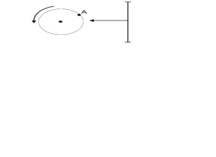
Figure 1: What is the probability that the rotating disk stops in such a way that the point $A$ will be exactly in front of the arrow?

However, the point $A$ can stop in front of the arrow, i.e., this event is not impossible and its probability should be strictly greater than zero, i.e., $P(E)>0$. The new approach allows us to calculate this probability numerically.

First of all, in order to state the experiment more rigorously, it is necessary to choose a numeral system to express the points on the circumference. This choice will fix the number of points, $K$, that we are able to distinguish on the circumference. Definition of the notion point allows us to define elementary events in our experiment as follows: the disk has stopped and the arrow indicates a point. As a consequence, we obtain that the number, $N(\Omega)$, of all possible elementary events, $e_{i}$, in our experiment is equal to $K$ where $\Omega=\cup_{i=1}^{N(\Omega)}e_{i}$ is the sample space of our experiment. If our disk is well balanced, all elementary events are equiprobable and, therefore, have the same probability equal to $\frac{1}{N(\Omega)}$. Thus, we can calculate $P(E)$ directly by subdividing the number, $N(E)$, of favorable elementary events by the number, $K=N(\Omega)$, of all possible events.

For example, if we use numerals of the type $\frac{i}{\mbox{\char 172}},i\in\mathbb{N},$ then $K=\mbox{\char 172}$. The number $N(E)$ depends on our decision about how many numerals we want to use to represent the point $A$. If we decide that the point $A$ on the circumference is represented by $m$ numerals we obtain

$$P(E)=\frac{N(E)}{N(\Omega)}=\frac{m}{K}=\frac{m}{\mbox{\char 172}}>0.$$

where the number $\frac{m}{\mbox{\char 172}}$ is infinitesimal if $m$ is finite. Note that this representation is very interesting also from the point of view of distinguishing the notions ‘point’ and ‘arc’. When $m$ is finite than we deal with a point, when $m$ is infinite we deal with an arc.

In the case we need a higher accuracy, we can choose, for instance, numerals of the type $i\mbox{\char 172}^{-2},1\leq i\leq\mbox{\char 172}^{2},$ for expressing points at the disk. Then it follows $K=\mbox{\char 172}^{2}$ and, as a result, we obtain $P(E)=m\mbox{\char 172}^{-2}>0$.

This example with the rotating disk, of course, is a particular instance of the general situation taking place in the traditional probability theory where the probability that a continuous random variable $X$ attains a given value $a$ is zero, i.e., $P(X=a)=0$. While for a discrete random variable one could say that an event with probability zero is impossible, this can not be said in the case of a continuous random variable. As we have shown by the example above, in our approach this situation does not take place because this probability can be expressed by infinitesimals. As a consequence, probabilities of such events can be computed and used in numerical models describing the real world (see [13] for a detailed discussion on the modelling continuity by infinitesimals in the framework of the approach using grossone).

Moreover, the obtained probabilities are not absolute, they depend on the accuracy chosen for the mathematical model describing the experiment. There is again a straight analogy with Physics where it is not possible to obtain results that have a precision higher than the accuracy of the measurement of the data. We also cannot obtained a precision that is higher than the precision of numerals used in the mathematical model.

Figure 2: It is possible to calculate and to distinguish areas of these two objects

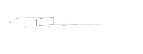
Figure 3: New possibilities for calculating volumes of objects

Let us now consider two examples showing that the new approach allows us to calculate areas and volumes of a more general class of objects than the traditional one. In Fig. 2 two figures are shown. The traditional approach tells us that both of them have area equal to one. In the new approach, if we use numerals of the type $i\mbox{\char 172}^{-1},i\in\mathbb{N},$ to express points within a unit interval, then the unit interval consists of ① points and in the plane each point has the infinitesimal area $\mbox{\char 172}^{-1}\cdot\mbox{\char 172}^{-1}=\mbox{\char 172}^{-2}$. As a consequence, this value will be our accuracy in calculating areas in this example. Suppose now that the vertical line added to the square at the right figure in Fig. 2 has the width equal to one point. Then we are able to calculate the area, $S_{2}$, of the right figure and it will be possible to distinguish it from the area, $S_{1}$, of the square on the left

$$S_{1}=1\cdot 1=1,\hskip 28.45274ptS_{2}=1\cdot 1+1\cdot\mbox{\char 172}^{-1}=1\mbox{\char 172}^{0}1\mbox{\char 172}^{-1}.$$

If the added vertical line has the width equal to three points then it follows

$$S_{2}=1\cdot 1+3\cdot\mbox{\char 172}^{-1}=1\mbox{\char 172}^{0}3\mbox{\char 172}^{-1}.$$

The volume of the figure shown in Fig. 3 is calculated analogously:

$$\hskip 28.45274ptV=1\cdot 1\cdot 1+1\cdot 1\cdot\mbox{\char 172}^{-1}+1\cdot\mbox{\char 172}^{-1}\cdot\mbox{\char 172}^{-1}=1\mbox{\char 172}^{0}1\mbox{\char 172}^{-1}1\mbox{\char 172}^{-2}.$$

If the accuracy of the considered numerals of the type $i\mbox{\char 172}^{-1},i\in\mathbb{N},$ is not sufficient, we can increase it by using, for instance, numerals of the type $i\mbox{\char 172}^{-2},1\leq i\leq\mbox{\char 172}^{2}$. Then the unit interval consists of $\mbox{\char 172}^{2}$ points and at the plane each point has the infinitesimal area $\mbox{\char 172}^{-2}\cdot\mbox{\char 172}^{-2}=\mbox{\char 172}^{-4}$. As a result, by a complete analogy to the previous case we obtain for lines having the width, for instance, equal to five points in all three dimensions that

$$S_{2}=1\cdot 1+5\cdot\mbox{\char 172}^{-2}=1\mbox{\char 172}^{0}5\mbox{\char 172}^{-2},$$

$$V=1\cdot 1\cdot 1+1\cdot 1\cdot 5\cdot\mbox{\char 172}^{-2}+1\cdot 5\cdot\mbox{\char 172}^{-2}\cdot 5\cdot\mbox{\char 172}^{-2}=1\mbox{\char 172}^{0}5\mbox{\char 172}^{-2}25\mbox{\char 172}^{-4}.$$

Finally, we conclude the paper by a remark that thanks to the new approach it becomes possible to measure fractal objects at infinity. A detailed discussion on measuring fractals by the introduced infinite and infinitesimal numbers can be found in [13, 14].

References

- [1] V. Benci and M. Di Nasso, Numerosities of labeled sets: a new way of counting, Advances in Mathematics 173 (2003), 50–67.
- [2] G. Cantor, Contributions to the founding of the theory of transfinite numbers, Dover Publications, New York, 1955.
- [3] J.H. Conway and R.K. Guy, The book of numbers, Springer-Verlag, New York, 1996.
- [4] P. Gordon, Numerical cognition without words: Evidence from Amazonia, Science 306 (2004), no. 15 October, 496–499.
- [5] K. Knopp, Theory and application of infinite series, Dover Publications, New York, 1990.
- [6] P.A. Loeb and M.P.H. Wolff, Nonstandard analysis for the working mathematician, Kluwer Academic Publishers, Dordrecht, 2000.
- [7] A. Robinson, Non-standard analysis, Princeton Univ. Press, Princeton, 1996.
- [8] Ya.D. Sergeyev, Arithmetic of infinity, Edizioni Orizzonti Meridionali, CS, 2003.
- [9] Ya.D. Sergeyev, Computer system for storing infinite, infinitesimal, and finite quantities and executing arithmetical operations with them, patent application 08.03.04, 2004.
- [10] , http://www.theinfinitycomputer.com, 2004.
- [11] , Mathematical foundations of the Infinity Computer, Annales UMCS Informatica AI 4 (2006), 20–33.
- [12] , Misuriamo l’infinito, Periodico di Matematiche 6(2) (2006), 11–26.
- [13] , Blinking fractals and their quantitative analysis using infinite and infinitesimal numbers, Chaos, Solitons Fractals 33(1) (2007), 50–75.
- [14] , Measuring fractals by infinite and infinitesimal numbers, Mathematical Methods, Physical Methods Simulation Science and Technology 1(1) (2008), 217–237.
- [15] , A new applied approach for executing computations with infinite and infinitesimal quantities, Informatica (2008), (to appear).
- [16] R.G. Strongin and Ya.D. Sergeyev, Global optimization and non-convex constraints: Sequential and parallel algorithms, Kluwer Academic Publishers, Dordrecht, 2000.
- [17] , Global optimization: Fractal approach and non-redundant parallelism, J. Global Optimization 27(1) (2003), 25–50.
- [18] G.W. Walster, Compiler support of interval arithmetic with inline code generation and nonstop exception handling, Tech. Report, Sun Microsystems, 2000.