q–deformed logistic map with delay feedback

Abstract

The delay logistic map with two types of q–deformations: Tsallis and Quantum–group type are studied. The stability of the map and its bifurcation scheme is analyzed as a function of the deformation and delay feedback parameters. Chaos is suppressed in a certain region of deformation and feedback parameter space. The steady state obtained by delay feedback is maintained in one type of deformation while chaotic behavior is recovered in another type with increasing delay.

I Introduction

Theory of quantum integrable systems vd85 ; mj85 has initiated a new type of symmetry and associated with it mathematical objects called quantum groups. These are related to the usual Lie groups as quantum mechanics is related to its classical limit. Physically a group quantization can lead to a kind of deformation of the group manifold, related to a physical (classical or quantum) system. q–deformation of many classical Lie groups has stimulated much activity in the pursuit of understanding its physical meaning, due to the emergence of quantum group like features in many physical systems. It has been realized that q–deformation effectively takes into account the interactions in physical systems ev92 ; cy91 ; cgy ; rp93 . The q–deformation is non-trivial in the sense that the emerging deformed algebra is no longer linear. It would be constructive to study q–deformation in the context of dynamical systems.

One of the popular model of discrete nonlinear dynamical systems is logistic map cd . The study of dynamical system with delay is important when the information is feedback with a measurable delay, e.g., due to the spatial extensiveness of the system and the finite velocity of propagation of information, or when the characteristic timescale of the system is smaller than the delay time r3 . The delayed equations have been used for modeling purposes in optics d1 ; d2 , chemistry d3 , and biological systems d4 ; d5 . The delay feedback also plays an important role in controlling chaos ogy ; pyragas . The interplay of delay and nonlinearity plays a central role in self-organization and complex phenomena of dynamical systems and chaos is suppressed or controlled by stabilizing unstable periodic orbits with delay feedback r2 ; r6 ; r1 ; r5 ; rd . In another work ar99 , the normal logistic and exponential maps were used to study the transition from chaotic to regular dynamics induced by stochastic driving.

A one-dimensional logistic map is a non-linear difference equation

$$x_{n+1}=\alpha x_{n}(1-x_{n}),$$ (1)

where $\alpha$ is a constant, and is taken to be positive in the rest of the paper. Also, $x_{n}$ denotes the value of $x$ after $n$ iterations. Eq. (1) arises, for e.g., in the case of modeling of population growth $\frac{dN(t)}{dt}=r(t)N(t)$, where $N(t)$ is the population at a time $t$ and $r(t)$ is the difference between birth and death rates per head of the population.

As q–deformation essentially involves modification of a function such that in the limit of $q\rightarrow 1$ the usual function is obtained, there is no unique q-deformation for a function. On the other hand, delay transforms the dynamical state of the system. It is therefore natural to use q-deformations suitably in the study of non-linear systems with delay feedback. Here we discuss two forms of q–deformations of the logistic map, studied in the literature, but with the additional proviso that the map has a memory inbuilt into it, in the form of a feedback mechanism. This has the advantage of studying the system from a more realistic perspective as well as the possibility of having a chaos suppression mechanism inbuilt into the system.

The paper is setup as follows. In Section II, we discuss the basic deformations, that will be studied, along with delay. The logistic equation deformed by the two prescriptions and undergoing a delayed feedback are studied in Sections III (A) and (B), respectively. Along with a numerical study of the interplay between the various parameters, a stability study of the two systems is also made. Section IV concludes the paper.

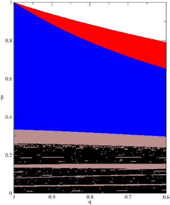
Figure 1: The parameter space ($\epsilon$, $\beta$) showing chaotic (black color), periodic (brown color for period $>$ 2 and blue for period 2), period 1 (non-zero steady state in blue color) and period 1 (zero steady state in white). Here nonlinearity parameter $\alpha=4$, delay parameter $\tau=1$. As seen from the figure, with increase in coupling ($\beta$), for fixed q-deformation $\epsilon$, the system undergoes a transition from the chaotic to the periodic regime, thereby highlighting the role played by the feedback on chaos suppression.

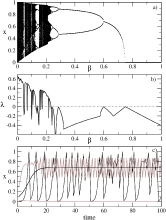
Figure 2: a) Bifurcation diagram depicting $x$ with respect to $\beta$ for $\alpha=4$, $\tau=1$. As seen from the figure, with increase in coupling ($\beta$), for fixed q-deformation $\epsilon=0.5$, the system undergoes a transition from the chaotic to the periodic regime, ultimately to the steady state, confirming the scenario depicted in Fig. (2) b), where the Lyapunov exponent $\lambda$ is plotted with respect to $\beta$ for $\alpha=4$, $\tau=1$. As seen from the figure, with increase in coupling ($\beta$), for fixed q-deformation $\epsilon$, the system undergoes a transition from the chaotic ($\lambda>0$) to the periodic ($\lambda<0$) regime, ultimately to the steady state. c) Time series showing chaotic, period-2 and steady states for $\beta=0.0$, $0.5$, $0.7$, and $0.8$ respectively.

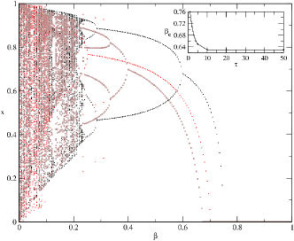
Figure 3: Bifurcation diagram depicting $x$ with respect to $\beta$ for $\alpha=4$ $q=0.5$, $\tau=1,2$ and $3$. System behavior is period two cycle, fixed point and chaotic for higher delay feedback strength for $\tau=1,2$ and $3$ respectively. In the inset, is plotted the critical value of the feedback parameter $\beta_{c}$, for which the system goes into the steady state $x^{\star}=0$.

II $q$–deformation with delay

A deformation of the logistic map (Eq. 1), based on the non-extensive statistics of Tsallis tsallis was proposed rs05 , in which the map

$$x_{n+1}=\alpha[x_{n}](1-[x_{n}]),$$ (2)

was considered. Here $[x]=\frac{x}{1+(1-q)(1-x)}$, and $-\infty<q<2$ for $x$ in the interval $[0,1]$. An important difference between (1) and (2) is that the deformed map (2) is concave in parts of $x$-space while the map without deformation (1) is always convex. Further, the use of (2) showed the rare phenomena of the co-existence of attractors, i.e., the co-existence of normal and chaotic behavior.

The logistic map with delay ($\tau$) feedback is given by:

$$x_{n+1}=f(x_{n})=\alpha x_{n}(1-x_{n})(1-\beta)+\beta x_{n-\tau}$$ (3)

where, $\beta$ is the feedback amplitude and $\tau$ is the delay time. The analogous q-deformed map with delay is:

$$x_{n+1}=\alpha[x_{n}](1-[x_{n}])(1-\beta)+\beta[x_{n-\tau}].$$ (4)

Another Quantum–group (Qu-group) type of q-deformation, of the logistic map, was proposed r02 as:

$$[x_{n+1}]=\alpha[x_{n}](1-[x_{n}]),$$ (5)

where

$$[x]=\frac{1-q^{x}}{1-q}.$$ (6)

Here $q$ is real and $x$ is in the interval $[0,1]$. This q-deformed logistic map is different from Eq. (2). It is not possible to transform the q-deformed map, introduced in Eq. (5), to that in Eq. (2). In particular, it is not possible to relate the $q$ parameter in Eq. (2) to the q parameter in Eq. (5). Further, in the proposed q–deformed map Eq. (5), the left hand side is also q-deformed, in contrast to Eq. (2). Thus in the space of q–deformed variables the q-deformed logistic map Eq. (5), is the usual map. In mapping to ordinary space, all the corresponding physical features emerge. This is not possible in the map Eq. (2). In the limit $q\rightarrow 1$, it is seen that $[x]\rightarrow x$ and we obtain the usual logistic map (1).

The corresponding deformed map with delay would be:

$$[x_{n+1}]=\alpha[x_{n}](1-[x_{n}])(1-\beta)+\beta[x_{n-\tau}].$$ (7)

What do we expect from such a study? q-deformations simulate correlations in the system while the delayed feedback brings in memory. An interplay of these two effects should help in understanding the mechanism of suppression of chaos in systems that have inbuilt correlations.

III Analysis of the $q$–deformed logistic map with delay

Here we take up the logistic map with delayed feedback and q-deformed according to both the prescriptions, i.e. according to Eqs. (2) (Tsallis type) and (5) (Qu-group type), respectively.

III.1 Tsallis type of deformation

III.1.1 Stability Analysis: Analytical Results

We make an analytical study of the effect of memory in Eq. (4). This involves expanding the original equation to a set of $\tau+1$ equations, $\tau$ being the delay r3 . In order to capture the essence of our q-deformed delayed logistic map, we take up the case of $\tau=1$. For the one-cycle stability, using Eq. (4):

$$x_{n+1}= \alpha(1-\beta)(2-q)\frac{x_{n}(1-x_{n})}{[1+(1-q)(1-x_{n})]^{2}}$$ (8)

$$+\beta\frac{y_{n}}{1+(1-q)(1-y_{n})},$$

$$y_{n+1}= x_{n}.$$

The corresponding Jacobian matrix takes the form:

$$J(x,y)=\left(\begin{array}[]{cc}\alpha(1-\beta)(2-q)\frac{2-q-(3-q)x_{n}}{[1+(1-q)(1-x_{n})]^{3}}&\frac{\beta(2-q)}{[1+(1-q)(1-y_{n})]^{2}}\\ 1&0\end{array}\right),$$ (9)

which for the trivial fixed point: $x=y=0$ gives:

$$J(0,0)=\left(\begin{array}[]{cc}\frac{\alpha(1-\beta)}{(2-q)}&\frac{\beta}{(2-q)}\\ 1&0\end{array}\right).$$ (10)

From the characteristic equation of Eq. (10), its eigenvalues are:

$$\lambda_{1,2}=\frac{\alpha(1-\beta)}{2(2-q)}\pm\frac{1}{2(2-q)}\sqrt{\alpha^{2}(1-\beta)^{2}+4\beta(2-q)}.$$ (11)

From the above eigenvalues, the condition for the stability of the fixed point is obtained as:

$$\beta>\frac{\alpha-(2-q)}{\alpha-1}.$$ (12)

These results are borne out by the numerical results shown below, where along with one-cycle stability, multi-cycle stability is also analyzed.

III.1.2 Numerical results

We fixed the nonlinearity parameter $\alpha=4$ and delay time $\tau=1$ to study the effect of q–deformation and delay feedback in $(q,\beta)$ parameter space as shown in Fig. 1. For lower feedback strength $\beta$, system is in chaotic (in black) or in higher period (in brown) state. With sufficiently large delay feedback, system goes to period two cycle (in blue) and then to steady state $x^{*}\neq 0$ (in red) and then to $x^{*}=0$ (in white). The bifurcation diagram and Lyapunov exponent as a function of feedback strength $\beta$ is plotted in Figs. 2(b) and (c), respectively, for fixed q-deformation $q=0.5$ which confirms chaos suppression via reverse period-doubling bifurcation. Time series in different dynamical states, i.e. chaotic, period two cycle, and steady states are shown in Fig. 2(c). When the delay time $\tau$ is further increased, the transition from chaos to steady state is seen to occur at lower values of feedback strength $\beta$ and the critical value of feedback strength $\beta_{c}$, when the system approaches the steady state $x^{*}=0$, is $0.76$ for $\tau=1$ and approaches to $0.63$ with increasing $\tau$ (see Fig. 3).

Thus, in the Tsallis-type of q-deformed logistic map with delay, with increase in feedback, stability is seen for all delays; in contrast to the situation in the corresponding map without deformation, where stability was observed for only odd delays r3 .

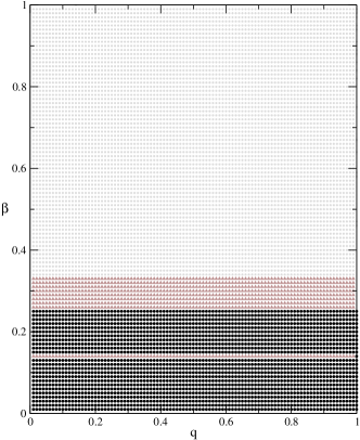
Figure 4: The parameter space ($q$, $\beta$) showing chaotic (black color) and periodic (brown for period $>$ 2 and gray for period 2). Here nonlinearity parameter $\alpha=4$, delay parameter $\tau=1$. As seen from the figure, with increase in coupling ($\beta$), for any given q-deformation $\epsilon$, the system undergoes a transition from the chaotic to the periodic–2 cycle regime, thereby highlighting the role played by the feedback on chaos suppression.

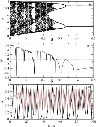
Figure 5: a) Bifurcation diagram depicting $x$ with respect to $\beta$ for $\alpha=4$, $\tau=1$. As seen from the figure, with increase in coupling ($\beta$), for fixed q-deformation $q=0.5$, the system undergoes a transition from the chaotic to the periodic–2 cycle regime confirming the scenario depicted in Fig. (4). b) Lyapunov exponent $\lambda$ with respect to $\beta$ for $\alpha=4$, $\tau=1$. As seen from the figure, with increase in coupling ($\beta$), for fixed q-deformation $q$, the system undergoes a transition from the chaotic ($\lambda>0$) to the periodic ($\lambda<0$) regime, ultimately to the period–2 cycle state. c) Time series showing chaotic and period-2 states for $\beta=0.0$ and $0.4$ respectively.

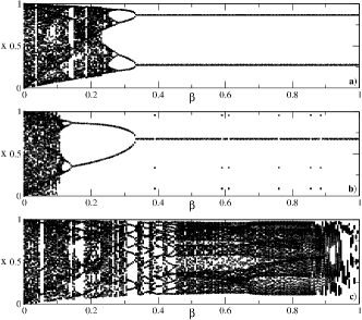
Figure 6: Bifurcation diagram depicting $x$ with respect to $\beta$ for $\alpha=4$ and $q=0.5$, for increasing delay time: $\tau=1,2$ and $3$, respectively. a) Period–2 cycle for $\tau=1$, b) fixed point for $\tau=2$, and c) chaotic behavior for $\tau=3$ are observed.

III.2 Quantum–group type of deformation

III.2.1 Stability Analysis: Analytical Results

We make an analytical study of the effect of memory in Eq. (7). As before, in order to capture the essence of our q-deformed delayed logistic map, we take up the case of $\tau=1$. For the one-cycle stability, using Eq. (7), we get the following two coupled equations:

$$X_{n+1} = 1-\frac{\alpha(1-\beta)}{(1-q)}(1-X_{n})(X_{n}-q)-\beta(1-Y_{n})$$

$$Y_{n+1} = X_{n},$$ (13)

where, for convenience in calculations, we have made the change in variable : $q^{x_{n}}=X_{n}$. The corresponding Jacobian matrix takes the form:

$$J(X,Y)=\left(\begin{array}[]{cc}\frac{\alpha(1-\beta)}{(1-q)}[2X_{n}-(q+1)]&\beta\\ 1&0\end{array}\right),$$ (14)

which for the trivial fixed point: $x=y=0$, corresponding in the new variables to: $X=Y=1$, gives:

$$J(0,0)=\left(\begin{array}[]{cc}\alpha(1-\beta)&\beta\\ 1&0\end{array}\right).$$ (15)

From the characteristic equation of Eq. (15), its eigenvalues are:

$$\lambda_{1,2}=\frac{\alpha(1-\beta)}{2}\pm\frac{1}{2}\sqrt{\alpha^{2}(1-\beta)^{2}+4\beta}.$$ (16)

From the above eigenvalues, the condition for the stability of the fixed point is obtained as:

$$\beta<1.$$ (17)

Since these calculations are made in the new variable $X_{n}$, which is related to the original variable $x_{n}$ by $x_{n}=\frac{\ln{X_{n}}}{\ln q}$; the result of Eq. (17) when interpreted in the original variable implies that $x^{*}=0$ will never stabilize under positive feedback. This is borne out by the numerical results shown below, where the one-cycle as well as multi-cycle stability is analyzed.

III.2.2 Numerical results

Again, we fixed the nonlinearity parameter $\alpha=4$ and delay time $\tau=1$ to study the effect of q–deformation and delay feedback in $(q,\beta)$ parameter space, as shown in Fig. 4. For lower feedback strength $\beta$, system is in chaotic (in black) or in higher period (in brown) state. With sufficiently large delay feedback, system goes to period two cycle (in gray). The bifurcation diagram and Lyapunov exponent as a function of feedback strength $\beta$ is plotted in Figs. 5(a) and (b), respectively for fixed q-deformation $q=0.5$ which confirms chaos suppression via reverse period-doubling bifurcation to period two–cycle. Time series in different dynamical states, i.e., chaotic and period two cycle are shown in Fig. 5(c). For delay time $\tau=2$, system goes to steady state with sufficient feedback strength and with further increase of delay time system goes back to chaotic state as shown in Fig. 6. For $\tau=2$, within period–1 cycle, some values of feedback strength $\beta$ take the system to period–3 cycle as shown in Fig. 6(b). It shows that chaos cannot be suppressed in Qu–group type of deformation for delay feedback with $\tau>2$. We have studied the asymmetric Qu–group type of deformation case ($x_{n+1}=f([x_{n}])$) also and find similar results (not shown here). Thus here the non-linearity is predominantly due to the form of the deformation chosen. In contrast to Tsallis type of deformation, the Qu-group type of deformation, suppress chaos to two-cycle as compared to one–cycle.

IV Conclusions

In this work, we have studied the logistic map from the perspective of q–deformation and delay feedback. This enables us to study the interplay between the competitive features, viz. complexity, brought by the q–deformation and order, by delay feedback. Chaos is suppressed with feedback for both kinds of deformations, i.e., Tsallis and Qu–group type. However, for the Tsallis type of deformation, a steady state is achieved, an observation which validates its use in statistical mechanics of complex systems, where one would expect a system to eventually go to a steady state, while for the Qu-group type of deformation the period–2 cycle gets stabilized. With increasing delay time, the transition to steady state is obtained at lower values of feedback strength in Tsallis type of q–deformation while chaotic state is recovered in Qu–group type of q–deformation with increasing delay time.

References

- (1) V. Drinfeld Dokl. Akad. Nauk. 283 1060 (1985).
- (2) M. Jimbo Lett. Math. Phys. 10 63 (1985).
- (3) G. J. Estere, C. Tejel and B. E. Villarroya J. Chem. Phys. 96 5614 (1992).
- (4) Z. Chang and H. Yan Phys. Lett. A 154 254 (1991).
- (5) Z. Chang, H. Y. Guo and H. Yan Phys. Lett. A 156 192 (1991).
- (6) Parthasarathy R 1993 IMSc-93/23, Preprint.
- (7) Jose J V and Saletan E J 2002 Classical Dynamics: A Contemporary Approach (Cambridge University Press)
- (8) T. Buchner , Phys. Rev. E 63, 016210 (2000).
- (9) K. Ikeda, Opt. Commun., 30, 257 (1979).
- (10) G. Giacomelli, R. Meucci, A. Politi, and F. T. Arecchi, Phys. Rev. Lett. 73, 1099 (1994).
- (11) I. R. Epstein, J. Chem. Phys., 92, 1702 (1990).
- (12) M. C. Mackey and L. Glass, Science, 197, 287 (1977).
- (13) S. Cavalcanti and E. Belardinelli, IEEE Trans. Biomed. Eng., 43, 982 (1996).
- (14) E. Ott, C. Grebogi, and Y. A. Yorke, Phys. Rev. Lett. 64, 1196 (1990).
- (15) K. Pyragas, Phys. Lett. A 170, 421 (1992).
- (16) M. de Sousa Vieira , Phys. Rev. E 54, 1200 (1996).
- (17) M. D. Shrimali, , Phys. Lett. A 374, 2636 (2010).
- (18) E. Fick , Phys. Rev. A 44, 2469 (1991).
- (19) C. Masoller , Phil. Trans. R. Soc. 369, 425, (2011).
- (20) Complex Time-Delay Systems. F. M. Atay (ed.), Springer-Verlag Berlin, 2010.
- (21) Prasad A and Ramaswamy R 1999 eprint:arXiv:chao-dyn/9911002
- (22) C Tsallis 1988, J. Stat. Phys. 52, 479; M Gell-Mann and C Tsallis (Eds.), Nonextensive entropy - Interdisciplinary applications (Oxford University Press, New York, 2004)
- (23) R. Jaganathan and S. Sinha, Phys. Lett. A 338 277 (2005).
- (24) S. Banerjee and R. Parthasarathy J. Phys. A: Math. Theor. 44 045104 (2011).