Probabilistic representation of fundamental solutions to $\frac{\partial u}{\partial t}=\kappa_{m}\frac{\partial^{m}u}{\partial x^{m}}$.

Abstract.

For the fundamental solutions of heat-type equations of order $n$ we give a general stochastic representation in terms of damped oscillations with generalized gamma distributed parameters. By composing the pseudo-process $X_{n}$ related to the higher-order heat-type equation with positively skewed stable r.v.’s $T^{j}_{\frac{1}{3}}$, $j=1,2,\ldots,n$ we obtain genuine r.v.’s whose explicit distribution is given for $n=3$ in terms of Cauchy asymmetric laws. We also prove that $X_{3}(T^{1}_{\frac{1}{3}}(\ldots(T^{n}_{\frac{1}{3}}(t))\ldots))$ has a stable asymmetric law.

1. Introduction

The problem of studying the form of fundamental solutions of higher-order heat equations of the form

(1.1) $$\frac{\partial u_{m}}{\partial t}(x,t)=\kappa_{m}\frac{\partial^{m}u_{m}}{\partial x^{m}}(x,t),\quad x\in\mathbb{R},\;t>0,\quad m\geq 2$$

with

$$u_{m}(x,0)=\delta(x)$$

where

$$\kappa_{m}=\left\{\begin{array}[]{ll}(-1)^{m/2+1}&\textrm{if }$m$\textrm{ is even}\\ \pm 1&\textrm{if }$m$\textrm{ is odd}\end{array}\right.$$

has been tackled in some particular cases by mathematicians of the caliber of Bernstein [3]; Lévy [7]; Pòlya [11] and Burwell [4]. By applying the steepest descent method some recent papers by Li and Wong [8], Accetta and Orsingher [1], Lachal [6] have explored the form of the fundamental solutions of equation (1.1). The aim of this note is to give an explicit representation of the solutions to (1.1) for the case where the order of the equation is odd, alternative to the inverse Fourier transform

(1.2) $$u_{m}(x,t)=\frac{1}{2\pi}\int_{\mathbb{R}}e^{-i\beta x+t(-i\beta)^{m}\kappa_{m}}d\beta$$

and capable of representing the sign-varying behavior of the fundamental solutions to (1.1). Our result is that the fundamental solutions to (1.1) have the probabilistic representation

(1.3) $$u_{2n+1}(x,t)=\frac{1}{x\pi}E\left[e^{-b_{n}xG^{2n+1}(1/t)}\sin\left(a_{n}xG^{2n+1}(1/t)\right)\right],\quad x\in\mathbb{R},\;t>0$$

in the odd-order case, and

(1.4) $$u_{2n}(x,t)=\frac{1}{\pi x}E\Big{[}\sin\left(xG^{2n}(1/t)\right)\Big{]},\quad x\in\mathbb{R},\;t>0$$

for the even-order case. In (1.3) and (1.4) by $G^{\gamma}(t)$ we denote the generalized gamma r.v. with density

$$g^{\gamma}(x,t)=\gamma\frac{x^{\gamma-1}}{t}\exp\left(-\frac{x^{\gamma}}{t}\right),\quad x,t>0,\;\gamma>0.$$

The parameters $a_{n},b_{n}$ appearing in (1.3) and (1.4) are

$$a_{n}=\cos\frac{\pi}{2(2n+1)},\quad b_{n}=\sin\frac{\pi}{2(2n+1)}.$$

Results (1.3) and (1.4) show that the fundamental solutions have an oscillating behavior which has been explored in several papers by many researchers. In our view our result represents a concluding picture of the solutions to higher-order heat equations. For all values of the degree $n$ of the equation (1.1) we have solutions which have the behavior of damped oscillations where the probabilistic ingredients (the generalized gamma or Weibull-type distributions) depend only on $n\in\mathbb{N}$. An alternative universal representation of the fundamental solution in the odd-order case reads

(1.5) $$u_{2n+1}(x,t)=-\frac{1}{\pi x}\sum_{k=1}^{\infty}\left(\frac{-x}{\sqrt[2n+1]{t}}\right)^{k}\frac{1}{k!}\sin\frac{n\pi k}{2n+1}\Gamma\left(1+\frac{k}{2n+1}\right).$$

Functions $u_{2n+1}$ display ascillations which fade off as the degree $2n+1$ of the equation increases. A special attention has been devoted to third-order equations where we have that

(1.6) $$u_{3}(x,t)= \frac{1}{\sqrt[3]{3t}}Ai\left(\frac{x}{\sqrt[3]{3t}}\right),\quad x\in\mathbb{R},\,t>0$$

(1.7) $$= \frac{3t}{\pi x}\int_{0}^{\infty}e^{-\frac{xy}{2}}\sin\left(\frac{\sqrt{3}}{2}xy\right)\,y^{2}e^{-ty^{3}}\,dy$$

(1.8) $$= -\frac{1}{\pi x}\sum_{k=1}^{\infty}\left(-\frac{x}{\sqrt[3]{t}}\right)^{k}\frac{1}{k!}\sin\frac{\pi k}{3}\Gamma\left(1+\frac{k}{3}\right).$$

In the fourth-order case (biquadratic heat-equation) in Orsingher and D’Ovidio [10] we have shown that

$$u_{4}(x,t)= \frac{1}{2\pi}\int_{-\infty}^{+\infty}e^{-\frac{y^{4}t}{2^{2}}}\cos\left(xy\right)dy$$

$$= \frac{1}{2\pi\sqrt{2t^{1/2}}}\sum_{k=0}^{\infty}\frac{(-1)^{k}}{(2k)!}\left(-\frac{\sqrt{2}|x|}{t^{1/4}}\right)^{2k}\Gamma\left(\frac{k}{2}+\frac{1}{4}\right).$$

In a recent paper we have shown that the composition of an odd-order pseudo-process $X_{2n+1}$ with a positivly skewed stable r.v. $T_{\frac{1}{2n+1}}$ of order $\frac{1}{2n+1}$ yields a genuine r.v. with asymmetric Cauchy distribution, that is

(1.9) $$Pr\{X_{\frac{1}{2n+1}}(T_{\frac{1}{2n+1}}(t))\in dx\}=\frac{t\cos\frac{\pi}{2(2n+1)}}{\pi\left[(x+t\sin\frac{\pi}{2(2n+1)})^{2}+t^{2}\cos^{2}\frac{\pi}{2(2n+1)}\right]}dx.$$

For $n=1$ from (1.9) we can extract a very interesting relationship for the Airy function which reads

$$Pr\{X_{\frac{1}{3}}(T_{\frac{1}{3}}(t))\in dx\}/dx=$$

$$\int_{0}^{\infty}\frac{1}{\sqrt[3]{3s}}Ai\left(\frac{x}{\sqrt[3]{3s}}\right)\frac{t}{s}\frac{1}{\sqrt[3]{3s}}Ai\left(\frac{t}{\sqrt[3]{3s}}\right)ds=\frac{\sqrt{3}}{2\pi}\frac{t}{x^{2}+xt+t^{2}}.$$

We show here that the $m$-times iterated pseudo-process (with $T^{j}_{\frac{1}{2n+1}}$, $j=1,2,\ldots,m$ independent stable r.v.’s)

$$Z_{m}(t)=X_{2n+1}(T^{1}_{\frac{1}{2n+1}}(T^{2}_{\frac{1}{2n+1}}(\ldots(T^{m}_{\frac{1}{2n+1}}(t))\ldots))),\quad t>0$$

is a stable r.v. of order $\frac{1}{(2n+1)^{m-1}}$ with characteristic function

(1.10) $$Ee^{i\beta Z_{m}(t)}=\exp\left[-t|\beta|^{\frac{1}{(2n+1)^{m-1}}}\left(\cos\frac{\pi}{2(2n+1)^{m}}+i\frac{\beta}{|\beta|}\sin\frac{\pi}{2(2n+1)^{m}}\right)\right].$$

We have also explored the connection between solutions of fractional equations

$$\frac{\partial^{\alpha}u}{\partial t^{\alpha}}+\frac{\partial u}{\partial x}=0,\quad x>0,\;t>0$$

with the solutions of higher-order heat-type equations (1.1) for $\alpha=\frac{1}{m}$, $m\in\mathbb{N}$.

2. Pseudo-processes

Some basic facts about the fundamental solutions of higher-order heat equations had been established many years ago essentially by applying the steepest descent method. In particular, Li and Wong [8] have shown that the number of zeros is infinite for solutions to even-order equations. The steepest descent method was applied by Accetta and Orsingher [1] for the analysis of the third-order equation. The oscillating behavior of the solutions of higher-order heat-type equations is confirmed by our analysis. Furthermore, for the odd-order case our results show that the asymmetry of solutions decreases as the order $2n+1$ increases. The result of Theorem 2.1 below shows that solutions of all odd-order heat equations can be constructed by means of damped oscillating functions with gamma distributed parameters.

We pass now to our principal result.

Theorem 2.1.

The solution to

(2.1) $$\left\{\begin{array}[]{ll}\frac{\partial u}{\partial t}=(-1)^{n}\frac{\partial^{2n+1}u}{\partial x^{2n+1}},&x\in\mathbb{R},\;t>0\\ u(x,0)=\delta(x)\end{array}\right.$$

is given by

(2.2) $$u_{2n+1}(x,t)=\frac{1}{x\pi}E\left[e^{-b_{n}xG^{2n+1}(1/t)}\sin\left(a_{n}xG^{2n+1}(1/t)\right)\right]$$

where, $\forall\,t>0$, the r.v. $G^{\gamma}(t)$ has the generalized gamma distribution

$$g^{\gamma}(x,t)=\gamma\frac{x^{\gamma-1}}{t}\exp\left(-\frac{x^{\gamma}}{t}\right),\quad x,t>0,\;\gamma>0.$$

and

$$a_{n}=\cos\frac{\pi}{2(2n+1)},\quad b_{n}=\sin\frac{\pi}{2(2n+1)}$$

Proof.

We start by evaluating the Fourier transform of (2.2)

(2.3) $$\int_{\mathbb{R}}e^{i\beta x}u_{2n+1}(x,t)dx$$

$$= \int_{\mathbb{R}}e^{i\beta x}dx\int_{0}^{\infty}\frac{(2n+1)t}{\pi x}e^{-b_{n}xw}\sin(a_{n}xw)w^{2n}e^{-tw^{2n+1}}dw$$

$$= (2n+1)t\int_{0}^{\infty}w^{2n}e^{-tw^{2n+1}}\int_{\mathbb{R}}\frac{e^{i\beta x+ia_{n}xw-b_{n}xw}-e^{i\beta x-ia_{n}xw-b_{n}xw}}{2\pi ix}dx\,dw$$

$$= (2n+1)t\int_{0}^{\infty}w^{2n}e^{-tw^{2n+1}}\left[H_{\beta}(w(a_{n}-ib_{n}))-H_{\beta}(-w(a_{n}+ib_{n}))\right]dw$$

where in the last step we used the integral representation of the Heaviside function

$$H_{y}(x)=-\frac{1}{2\pi}\int_{\mathbb{R}}e^{-iwx}\frac{e^{iyw}}{iw}dw=\frac{1}{2\pi}\int_{\mathbb{R}}e^{iwx}\frac{e^{-iyw}}{iw}dw$$

By a change of variable, the Fourier transform (2.3) takes the form

$$\int_{\mathbb{R}}e^{i\beta x}u_{2n+1}(x,t)dx= \frac{(2n+1)t}{(a_{n}-ib_{n})^{2n+1}}\int_{0}^{\infty}w^{2n}e^{-t\left(\frac{w}{a_{n}-ib_{n}}\right)^{2n+1}}H_{\beta}(w)dw$$

$$-\frac{(2n+1)t}{(a_{n}+ib_{n})^{2n+1}}\int_{0}^{\infty}w^{2n}e^{-t\left(\frac{w}{a_{n}+ib_{n}}\right)^{2n+1}}H_{\beta}(-w)dw$$

$$= i(2n+1)t\int_{0}^{\infty}w^{2n}e^{-itw^{2n+1}}H_{\beta}(w)dw$$

$$+i(2n+1)t\int_{0}^{\infty}w^{2n}e^{itw^{2n+1}}H_{\beta}(-w)dw$$

$$= i(2n+1)t\int_{-\infty}^{+\infty}w^{2n}e^{-itw^{2n+1}}H_{\beta}(w)dw$$

(2.4) $$= i(2n+1)t\int_{\beta}^{+\infty}w^{2n}e^{-itw^{2n+1}}dw.$$

In the above steps we used the fact that

$$(a_{n}+ib_{n})^{2n+1}=i,\quad\textrm{and}\quad(a_{n}-ib_{n})^{2n+1}=-i.$$

The integral (2.4) can be performed in two different ways. First we can take the Laplace transform

$$\int_{0}^{\infty}e^{-\mu t}\left(\int_{\mathbb{R}}e^{i\beta x}u_{2n+1}(x,t)dx\right)dt= \int_{\beta}^{\infty}w^{2n}\int_{0}^{\infty}e^{-(\mu+iw^{2n+1})t}it(2n+1)dt\,dw$$

$$= \int_{\beta}^{\infty}\frac{i(2n+1)w^{2n}dw}{(\mu+iw^{2n+1})^{2}}$$

$$= \frac{1}{\mu+i\beta^{2n+1}}$$

$$= \int_{0}^{\infty}e^{-\mu t}e^{-it\beta^{2n+1}}dt.$$

This shows that

$$\int_{-\infty}^{+\infty}e^{i\beta x}u_{2n+1}(x,t)dx=e^{-it\beta^{2n+1}}.$$

We can arrive at the some result by means of the following trick

$$\int_{-\infty}^{+\infty}e^{i\beta x}u_{2n+1}(x,t)dx= \lim_{\mu\to 0}\left[i(2n+1)t\int_{\beta}^{\infty}w^{2n}e^{-itw^{2n+1}-\mu w^{2n+1}}dw\right]$$

$$= \lim_{\mu\to 0}\frac{it}{\mu+it}e^{-(it+\mu)\beta^{2n+1}}$$

$$= e^{-it\beta^{2n+1}}.$$

We have thus shown that the Fourier transform of (2.2) coincides with the Fourier transform of the solution to the Cauchy problem (2.1). ∎

For the special case of the third-order heat equation we have the following result.

Theorem 2.2.

The solution of the Cauchy problem

(2.5) $$\left\{\begin{array}[]{ll}\frac{\partial u}{\partial t}=-\frac{\partial^{3}u}{\partial x^{3}},\quad x\in\mathbb{R},\,t>0\\ u(x,0)=\delta(x)\end{array}\right.$$

can be written as

(2.6) $$u_{3}(x,t)= \frac{1}{x\pi}E\left[e^{-\frac{x}{2}G^{3}(1/t)}\sin\left(\frac{3^{1/2}x}{2}G^{3}(1/t)\right)\right]$$

(2.7) $$= \frac{3t}{\pi x}\int_{0}^{\infty}e^{-\frac{xy}{2}}\sin\left(\frac{\sqrt{3}}{2}xy\right)\,y^{2}e^{-ty^{3}}\,dy$$

(2.8) $$= \frac{1}{\sqrt[3]{3t}}Ai\left(\frac{x}{\sqrt[3]{3t}}\right),\quad x\in\mathbb{R},\,t>0.$$

Proof.

It is convenient to work with the following series expansion of the Airy function (see Orsingher and Beghin [9, formula (4.10)])

(2.9) $$Ai(w)= \frac{3^{-2/3}}{\pi}\sum_{k\geq 0}(3^{1/3}w)^{k}\frac{\sin\left(2\pi(k+1)/3\right)}{k!}\Gamma\left(\frac{k+1}{3}\right)$$

$$= \frac{3^{-2/3}}{\pi}\sum_{k\geq 1}(3^{1/3}w)^{k-1}\frac{\sin\left(2\pi k/3\right)}{(k-1)!}\Gamma\left(\frac{k}{3}\right)$$

$$= \frac{1}{w\pi}\sum_{k\geq 1}(3^{1/3}w)^{k}\frac{\sin\left(2\pi k/3\right)}{k!}\Gamma\left(\frac{k}{3}+1\right).$$

If we expand the function

(2.10) $$g(x,\phi)= e^{x\cos\phi}\sin\left(x\sin\phi\right)=e^{x\cos\phi}\frac{e^{ix\sin\phi}-e^{-ix\sin\phi}}{2i}$$

$$= \frac{e^{xe^{i\phi}}-e^{xe^{-i\phi}}}{2i}=\frac{1}{2i}\left[\sum_{k=0}^{\infty}\frac{\left(xe^{i\phi}\right)^{k}}{k!}-\sum_{k=0}^{\infty}\frac{\left(xe^{-i\phi}\right)^{k}}{k!}\right]$$

$$= \sum_{k=0}^{\infty}\frac{x^{k}}{k!}\frac{e^{i\phi k}-e^{-i\phi k}}{2i}=\sum_{k=0}^{\infty}\frac{x^{k}}{k!}\sin\phi k$$

we establish a relationship which is useful in transforming (2.9) as

$$Ai(w)= \frac{1}{w\pi}\sum_{k\geq 1}(3^{1/3}w)^{k}\frac{\sin\left(2\pi k/3\right)}{k!}\Gamma\left(\frac{k}{3}+1\right)$$

$$= \frac{1}{w\pi}\sum_{k\geq 1}(3^{1/3}w)^{k}\frac{\sin\left(2\pi k/3\right)}{k!}\int_{0}^{\infty}z^{k/3}e^{-z}dz$$

$$= \frac{1}{w\pi}\int_{0}^{\infty}e^{-z}\sum_{k\geq 1}((3z)^{1/3}w)^{k}\frac{\sin\left(2\pi k/3\right)}{k!}\,dz$$

$$= \frac{1}{w\pi}\int_{0}^{\infty}e^{-z}e^{-(3z)^{1/3}w/2}\sin\left(\frac{3^{5/6}}{2}z^{1/3}w\right)\,dz.$$

Now we write

(2.11) $$\frac{1}{(3t)^{1/3}}Ai\left(\frac{x}{(3t)^{1/3}}\right)= \frac{3t}{x\pi}\int_{0}^{\infty}z^{2}\exp\left(-z^{3}t-\frac{zx}{2}\right)\sin\left(\frac{3^{1/2}}{2}z\,x\right)\,dz.$$

From (2.2), for $n=1$ ($\gamma=3$), we write

$$u_{3}(x,t)= \frac{3t}{\pi x}\int_{0}^{\infty}e^{-xz\sin\frac{\pi}{6}}\sin\left(xz\cos\frac{\pi}{6}\right)\,z^{2}e^{-tz^{3}}\,dz$$

$$= (z^{3}t=y)=\frac{1}{\pi x}\int_{0}^{\infty}e^{-y}e^{-\frac{x}{2}\sqrt[3]{\frac{y}{t}}}\sin\left(\frac{\sqrt{3}}{2}x\sqrt[3]{\frac{y}{t}}\right)dy.$$

This proves, in a different way, that

$$u_{3}(x,t)=\frac{1}{\sqrt[3]{3t}}Ai\left(\frac{x}{\sqrt[3]{3t}}\right).$$

∎

Theorem 2.3.

We can write the fundamental solution $u_{2n+1}$ in the following alternative form

(2.12) $$u_{2n+1}(x,t)=-\frac{1}{\pi x}\sum_{k=1}^{\infty}\left(\frac{-x}{\sqrt[2n+1]{t}}\right)^{k}\frac{1}{k!}\sin\frac{n\pi k}{2n+1}\Gamma\left(1+\frac{k}{2n+1}\right)$$

Proof.

From (2.2) we have that

$$u_{2n+1}(x,t)= \frac{(2n+1)t}{\pi x}\int_{0}^{\infty}e^{-xy\sin\frac{\pi}{2(2n+1)}}\sin\left(xy\cos\frac{\pi}{2(2n+1)}\right)y^{2n}e^{-ty^{2n+1}}dy$$

$$= \frac{(2n+1)t}{\pi x}\int_{0}^{\infty}e^{-xy\cos\frac{n\pi}{(2n+1)}}\sin\left(xy\sin\frac{n\pi}{(2n+1)}\right)y^{2n}e^{-ty^{2n+1}}dy$$

$$= (\textrm{by }\eqref{uno11})=-\frac{(2n+1)t}{\pi x}\int_{0}^{\infty}y^{2n}e^{-ty^{2n+1}}\sum_{k=0}^{\infty}\frac{(-xy)^{k}}{k!}\sin\frac{n\pi k}{2n+1}dy$$

$$= -\frac{1}{\pi x}\sum_{k=0}^{\infty}\left(\frac{-x}{t^{\frac{1}{2n+1}}}\right)^{k}\frac{1}{k!}\sin\left(\frac{n\pi k}{2n+1}\right)\Gamma\left(1+\frac{k}{2n+1}\right)$$

∎

Remark 2.4.

We note that

$$u_{2n+1}(0,t)=\frac{1}{\pi t^{\frac{1}{2n+1}}}\sin\left(\frac{n\pi}{2n+1}\right)\Gamma\left(1+\frac{1}{2n+1}\right)\stackrel{{\scriptstyle n\to\infty}}{{\longrightarrow}}\frac{1}{\pi}$$

Remark 2.5.

We are able to evaluate the semi-infinite integral

$$\int_{0}^{\infty}u_{2n+1}(x,t)\,dx$$

by means of the representation (2.2). Indeed, by considering that

(2.13) $$\int_{0}^{\infty}\frac{e^{-Bx}}{x}\sin\left(Ax\right)\,dx= \operatorname{arctan}\left(\frac{A}{B}\right)$$

$$= \frac{\pi}{2}-\operatorname{arccot}\left(\frac{A}{B}\right)$$

(see Gradshteyn and Ryzhik [5, formula 3.941]) we get that

$$\int_{0}^{\infty}u_{2n+1}(x,t)\,dx= \int_{0}^{\infty}\frac{1}{x\pi}E\left[e^{-bxG^{2n+1}(1/t)}\sin\left(axG^{2n+1}(1/t)\right)\right]\,dx$$

$$= \frac{1}{\pi}\left[\frac{\pi}{2}-\operatorname{arccot}\left(\frac{a}{b}\right)\right]$$

$$= \frac{1}{\pi}\left[\frac{\pi}{2}-\operatorname{arccot}\left(\frac{\cos\frac{\pi}{2}\frac{1}{2n+1}}{\sin\frac{\pi}{2}\frac{1}{2n+1}}\right)\right]$$

(2.14) $$= \frac{1}{2}\left[1-\frac{1}{2n+1}\right].$$

which is in accord with Lachal [6, formula 11].

Theorem 2.6.

The solution to

(2.15) $$\frac{\partial u}{\partial t}=(-1)^{n+1}\frac{\partial^{2n}u}{\partial x^{2n}},\quad x\in\mathbb{R},\;t>0$$

with initial condition $u(x,0)=\delta(x)$ can be written as

(2.16) $$u_{2n}(x,t)=\frac{1}{\pi x}E\Big{[}\sin\left(xG^{2n}(1/t)\right)\Big{]}$$

Proof.

The solution to (2.15) is given by

$$u_{2n}(x,t)=\frac{1}{\pi}\int_{0}^{\infty}e^{-t\beta^{2n}}\cos\beta x\,d\beta.$$

By integrating by parts we get that

$$u_{2n}(x,t)=\frac{\sin\beta x}{\pi x}e^{-t\beta^{2n}}\Bigg{|}_{0}^{\infty}+\frac{2nt}{\pi x}\int_{0}^{\infty}\beta^{2n-1}e^{-t\beta^{2n}}\sin\beta x\,d\beta$$

and this concludes the proof. ∎

Remark 2.7.

The solution (2.16) takes the following values in the origin

$$u_{2n}(0,t)=\frac{1}{\pi}EG^{2n}(1/t)=\frac{1}{\pi t^{1/2n}}\Gamma\left(1+\frac{1}{2n}\right)\stackrel{{\scriptstyle n\to\infty}}{{\longrightarrow}}\frac{1}{\pi}.$$

Clearly, in force of the symmetry and by considering formula (2.13), we obtain that

$$\int_{0}^{\infty}u_{2n}(x,t)dx=\frac{1}{2}.$$

Remark 2.8.

It is well-known that the solution to the fractional diffusion equation

(2.17) $$\left\{\begin{array}[]{l}\frac{\partial^{\nu}u}{\partial t^{\nu}}=\lambda^{2}\frac{\partial^{2}u}{\partial x^{2}},\quad x\in\mathbb{R},\;t>0,\nu\in(0,2]\\ u(x,0)=\delta(x)\end{array}\right.$$

with

$$u_{t}(x,0)=0\quad\textrm{for}\quad\nu\in(1,2]$$

is given by

$$u_{\nu}(x,t)= \frac{1}{2\lambda t^{\nu/2}}W_{-\frac{\nu}{2},1-\frac{\nu}{2}}\left(-\frac{|x|}{\lambda t^{\nu/2}}\right)$$

$$= \frac{1}{2\lambda t^{\nu/2}}\sum_{k=0}^{\infty}\frac{1}{k!}\left(-\frac{|x|}{\lambda t^{\nu/2}}\right)\frac{1}{\Gamma\left(1-\frac{\nu}{2}(1+k)\right)}$$

$$= \frac{1}{2\pi\lambda t^{\nu/2}}\sum_{k=0}^{\infty}\frac{1}{k!}\left(-\frac{|x|}{\lambda t^{\nu/2}}\right)\Gamma\left(\frac{\nu}{2}(1+k)\right)\sin\left(\frac{\pi\nu}{2}(1+k)\right).$$

The folded solution to the equation (2.17) reads

$$\bar{u}_{\nu}(x,t)=\left\{\begin{array}[]{ll}2u_{\nu}(x,t),&x\geq 0\\ 0,&x<0\end{array}\right.$$

and for $\nu=2\alpha$, $\alpha\in(0,1)$, $\lambda=1$ becomes

(2.18) $$q_{\alpha}(x,t)= \frac{1}{\pi t^{\alpha}}\sum_{r=0}^{\infty}\left(-\frac{x}{t^{\alpha}}\right)^{r}\frac{\Gamma(\alpha(r+1))}{r!}\sin\left(\pi\alpha(r+1)\right).$$

This represents a probability density of a r.v. $X(t)$ on the half-line $(0,\infty)$ which can be expressed in terms of positively skewed stable densities.

$$Pr\{X(t)\in dx\}= q_{\alpha}(x,t)dx=\left(\frac{x}{t^{\alpha}}=\frac{t}{y^{\alpha}}\right)=q_{\alpha}\left(\frac{t^{\alpha+1}}{y^{\alpha+1}}\right)\frac{\alpha t^{\alpha+1}}{y^{\alpha+1}}dy$$

$$= \frac{1}{\pi t^{\alpha}}\sum_{k=0}^{\infty}\frac{1}{k!}\left(-\frac{t}{y^{\alpha}}\right)^{k}\Gamma(\alpha(1+k))\sin\left(\pi\alpha(1+k)\right)\frac{\alpha t^{\alpha+1}}{y^{\alpha+1}}dy$$

$$= \frac{\alpha t}{\pi y^{\alpha+1}}\sum_{k=0}^{\infty}\frac{1}{k!}\left(-\frac{t}{y^{\alpha}}\right)^{k}\Gamma(\alpha(1+k))\sin\left(\pi\alpha(1+k)\right)dy$$

$$= \frac{\alpha}{\pi}\sum_{k=0}^{\infty}\frac{1}{k!}\Gamma(\alpha(1+k))y^{-\alpha(k+1)-1}t^{k+1}\sin\left(\pi\alpha(1+k)\right)dy$$

$$= p_{\alpha}(y,\alpha,t)\,dy$$

where in the last step the expression of the stable density

(2.19) $$p_{\alpha}(x,\alpha,1)=\frac{\alpha}{\pi}\sum_{k=0}^{\infty}\frac{1}{k!}\Gamma(\alpha(1+k))x^{-\alpha(1+k)-1}\sin(\pi\alpha(1+k)),\quad x\in\mathbb{R}_{+}.$$

The calculations above show that the r.v. $X(t)$ with distribution (2.18) can be expressed as

$$X(t)=t\left(\frac{t}{Y(t)}\right)^{\alpha}$$

where $Y(t)$ is a positively skewed stable-distributed r.v. of order $\alpha\in(0,1)$. In other words the stable law of $Y(t)$ is related to the folded solution of the fractional diffusion equation $X(t)$ in the sense that

$$Y(t)\stackrel{{\scriptstyle i.d.}}{{=}}t\left(\frac{t}{X(t)}\right)^{1/\alpha}.$$

This is because

$$Pr\left\{Y(t)<y\right\}=Pr\left\{X(t)>\frac{t^{\alpha+1}}{y^{\alpha}}\right\}=\int_{\frac{t^{\alpha+1}}{y^{\alpha}}}^{\infty}p_{\alpha}(x,\alpha,t)dx.$$

We give also the Laplace transforms with respect to time $t$ and space $x$ of $q_{\alpha}(x,t)$

(2.20) $$\int_{0}^{\infty}e^{-\lambda x}q_{\alpha}(x,t)dx= -\left[-\frac{1}{\lambda t^{\alpha}}E_{-\alpha,1-\alpha}\left(-\frac{1}{\lambda t^{\alpha}}\right)\right]$$

$$= E_{\alpha,1}(-\lambda t^{\alpha}),\quad t>0$$

where in the last step, formula

$$-\frac{1}{x}E_{-\alpha,1-\alpha}\left(\frac{1}{x}\right)=E_{\alpha,1}(x)$$

has been applied (see formula $(5.1)$ of Beghin and Orsingher [2]). Furthermore,

(2.21) $$\int_{0}^{\infty}e^{-\mu t}q_{\alpha}(x,t)dt=\mu^{\alpha-1}e^{-x\mu^{\alpha}},\quad x>0.$$

Formulas above help to check that $q_{\alpha}$ satisfies the fractional equation

(2.22) $$\frac{\partial^{\alpha}u}{\partial t^{\alpha}}+\frac{\partial u}{\partial x}=0$$

with iniital condition $u(x,0)=\delta(x)$ where $\frac{\partial^{\alpha}}{\partial t^{\alpha}}$ is the Caputo fractional derivative.

Remark 2.9.

The double Laplace transform of (2.22) reads

(2.23) $$\mu^{\alpha}\mathcal{L}(\lambda,\mu)-\mu^{\alpha-1}=\mathcal{L}(\lambda,\mu)$$

where

$$\mathcal{L}(\lambda,\mu)=\int_{0}^{\infty}e^{-\mu t}\int_{0}^{\infty}e^{-\lambda x}q_{\alpha}(x,t)\,dx\,dt.$$

Since

(2.24) $$\mathcal{L}(\lambda,\mu)=\frac{\mu^{\alpha-1}}{\mu^{\alpha}+\lambda}$$

the $t$-inverse Laplace transform is (2.20) while the $x$-inverse Laplace transform can be obtained from (2.24) as

(2.25) $$\frac{\mu^{\alpha-1}}{\mu^{\alpha}+\lambda}=\mu^{\alpha-1}\int_{0}^{\infty}e^{-x(\lambda+\mu^{\alpha})}dx.$$

Remark 2.10.

For $\alpha=1/2$, the formula (2.19) yields

$$p_{1/2}(x;1/2,1)= \frac{1}{2\pi}\sum_{r=0}^{\infty}(-1)^{r}\frac{\Gamma((r+1)/2)}{r!}x^{-\frac{(r+1)}{2}-1}\sin\left(\pi(r+1)/2\right)$$

$$= \frac{1}{2\pi}\sum_{k=0}^{\infty}\left[\frac{\Gamma\left(k+\frac{1}{2}\right)}{(2k)!}x^{-k-\frac{3}{2}}\sin\left(\pi k+\frac{\pi}{2}\right)-\frac{\Gamma(k)}{(2k-1)!}x^{-k-1}\sin\left(\pi k\right)\right]$$

$$= \frac{1}{2\pi x^{3/2}}\sum_{k=0}^{\infty}\frac{\Gamma\left(k+\frac{1}{2}\right)}{(2k)!}x^{-k}\sin\left(\pi k+\frac{\pi}{2}\right)$$

$$= \frac{1}{2\pi x^{3/2}}\sum_{k=0}^{\infty}(-1)^{k}\frac{\Gamma\left(k+\frac{1}{2}\right)}{(2k)!}x^{-k}$$

$$= \frac{1}{2\pi x^{3/2}}\sum_{k=0}^{\infty}\frac{(-1)^{k}}{(2k)!}2^{1-2k}\frac{\Gamma(2k)}{\Gamma(k)}\sqrt{\pi}x^{-k}$$

$$= \frac{1}{2\sqrt{\pi}x^{3/2}}\sum_{k=0}^{\infty}\frac{(-1)^{k}}{k!}2^{-2k}x^{-k}$$

(2.26) $$= \frac{1}{\sqrt{4\pi x^{3}}}\exp\left(-\frac{1}{4x}\right).$$

The result (2.26) shows that the stable law (2.19) for $\alpha=1/2$ coincides with the first-passage time of a standard Brownian motion through level $1/\sqrt{2}$.

Remark 2.11.

Two solutions to the third-order p.d.e

(2.27) $$\frac{\partial u}{\partial t}=-\frac{\partial^{3}u}{\partial x^{3}}$$

are given by

$$p(x,t)= \frac{1}{\sqrt[3]{3t}}Ai\left(\frac{x}{\sqrt[3]{3t}}\right)$$

and

$$q(x,t)= \frac{x}{t}\frac{1}{\sqrt[3]{3t}}Ai\left(\frac{x}{\sqrt[3]{3t}}\right)=\frac{x}{t}p(x,t).$$

Indeed, we have that

$$\frac{\partial q}{\partial t}(x,t)= -\frac{x}{t^{2}}p(x,t)+\frac{x}{t}\frac{\partial p}{\partial t}(x,t)$$

and

$$\frac{\partial q}{\partial x}(x,t)= \frac{1}{t}p(x,t)+\frac{x}{t}\frac{\partial p}{\partial x}(x,t),$$

$$\frac{\partial^{2}q}{\partial x^{2}}(x,t)= \frac{2}{t}\frac{\partial p}{\partial x}(x,t)+\frac{x}{t}\frac{\partial^{2}p}{\partial x^{2}}(x,t),$$

$$\frac{\partial^{3}q}{\partial x^{3}}(x,t)= \frac{3}{t}\frac{\partial^{2}p}{\partial x^{2}}(x,t)+\frac{x}{t}\frac{\partial^{3}p}{\partial x^{3}}(x,t),$$

$$= \frac{3}{t}\frac{\partial^{2}p}{\partial x^{2}}(x,t)-\frac{x}{t}\frac{\partial p}{\partial t}(x,t)$$

and therefore

$$\frac{\partial q}{\partial t}(x,t)+\frac{\partial^{3}q}{\partial x^{3}}(x,t)=\frac{1}{t^{2}}\left(3t\frac{\partial^{2}p}{\partial x^{2}}(x,t)-xp(x,t)\right).$$

By observing that

$$\frac{\partial^{2}}{\partial x^{2}}\left[\frac{1}{\sqrt[3]{3t}}y\left(\frac{x}{\sqrt[3]{3t}}\right)\right]=\frac{1}{3t}y^{\prime\prime}(z)\Bigg{|}_{z=\frac{x}{\sqrt[3]{3t}}}=\frac{1}{3t}y^{\prime\prime}\left(\frac{x}{\sqrt[3]{3t}}\right)$$

and the fact that

$$y^{\prime\prime}(z)-zy(z)=0$$

that is, $y$ satisfies the Airy equation, we get that

$$\frac{\partial q}{\partial t}(x,t)+\frac{\partial^{3}q}{\partial x^{3}}(x,t)=0.$$

By recursive arguments it can be shown that

(2.28) $$f_{m}(x,t)=\left(\frac{x}{t}\right)^{m}\frac{1}{\sqrt[3]{3t}}Ai\left(\frac{x}{\sqrt[3]{3t}}\right)$$

is also a solution to (2.27) for $m>1$.

Remark 2.12.

We have shown in a previous paper that the r.v.

(2.29) $$Z(t)=X_{3}(T_{\frac{1}{3}}(t))$$

obtained by composing the third-order pseudo-process $X_{3}$ with the stable subordinator $T_{\frac{1}{3}}$ with distribution

(2.30) $$Pr\{T_{\frac{1}{3}}(t)\in ds\}=ds\frac{t}{s}\frac{1}{\sqrt[3]{3s}}Ai\left(\frac{t}{\sqrt[3]{3s}}\right),\quad s,t>0$$

possesses Cauchy distribution

$$Pr\{Z(t)\in dx\}= dx\int_{0}^{\infty}\frac{1}{\sqrt[3]{3s}}Ai\left(\frac{x}{\sqrt[3]{3s}}\right)\frac{t}{s}\frac{1}{\sqrt[3]{3s}}Ai\left(\frac{t}{\sqrt[3]{3s}}\right)ds$$

$$= dx\frac{\sqrt{3}t}{2\pi(x^{2}+xt+t^{2})}$$

(2.31) $$= dx\frac{\sqrt{3}}{2\pi}\frac{t}{(x+\frac{t}{2})^{2}+\frac{3}{4}t^{2}}.$$

Result (2.31) shows that (2.29) is a genuine r.v..The characteristic function of (2.31) is clearly

(2.32) $$\int_{-\infty}^{+\infty}e^{i\beta x}Pr\{Z(t)\in dx\}=e^{-\frac{\sqrt{3}}{2}t|\beta|-i\frac{t}{2}\beta}.$$

We have now the following generalization of the previous result for the composition of the pseudo-process $X_{3}$ with successively composed subordinators of order $\frac{1}{3}$.

Theorem 2.13.

The r.v.

(2.33) $$Z_{n}(t)=X_{3}(T^{1}_{\frac{1}{3}}(\ldots(T^{n}_{\frac{1}{3}}(t))\ldots))$$

with $T^{j}_{\frac{1}{3}}$, $j=1,2,\ldots,n$, independent, positively skewed r.v.’s with law (2.30) has characteristic function

$$Ee^{i\beta Z_{n}(t)}= \exp\left[-t|\beta|^{\frac{1}{3^{n-1}}}\left(\cos\frac{\pi}{2\cdot 3^{n}}+i\,sgn(\beta)\,\sin\frac{\pi}{2\cdot 3^{n}}\right)\right]$$

(2.34) $$= \exp\left[-t|\beta|^{\frac{1}{3^{n-1}}}\cos\frac{\pi}{2\cdot 3^{n}}\left(1+i\,sgn(\beta)\,\tan\frac{\pi}{2\cdot 3^{n}}\right)\right]$$

Proof.

We first observe that

$$Pr\{Z_{n}(t)\in dx\}/dx$$

$$= \int_{0}^{\infty}\ldots\int_{0}^{\infty}\frac{1}{\sqrt[3]{3s_{1}}}Ai\left(\frac{x}{\sqrt[3]{3s_{1}}}\right)\frac{s_{2}}{s_{1}}\frac{1}{\sqrt[3]{3s_{1}}}Ai\left(\frac{s_{2}}{\sqrt[3]{3s_{1}}}\right)\ldots\frac{t}{s_{n}}\frac{1}{\sqrt[3]{3s_{n}}}Ai\left(\frac{t}{\sqrt[3]{3s_{n}}}\right)\prod_{j=1}^{n}ds_{j}$$

has Fourier transform

$$\int_{-\infty}^{+\infty}e^{i\beta x}Pr\{Z_{n}(t)\in dx\}$$

$$= \int_{0}^{\infty}\ldots\int_{0}^{\infty}e^{-i\beta^{3}s_{1}}\;\frac{s_{2}}{s_{1}}\frac{1}{\sqrt[3]{3s_{1}}}Ai\left(\frac{s_{2}}{\sqrt[3]{3s_{1}}}\right)\ldots\frac{t}{s_{n}}\frac{1}{\sqrt[3]{3s_{n}}}Ai\left(\frac{t}{\sqrt[3]{3s_{n}}}\right)\prod_{j=1}^{n}ds_{j}$$

$$= \int_{0}^{\infty}\ldots\int_{0}^{\infty}e^{-(i\beta^{3})^{\frac{1}{3}}s_{2}}\;\frac{s_{3}}{s_{2}}\frac{1}{\sqrt[3]{3s_{2}}}Ai\left(\frac{s_{3}}{\sqrt[3]{3s_{2}}}\right)\ldots\frac{t}{s_{n}}\frac{1}{\sqrt[3]{3s_{n}}}Ai\left(\frac{t}{\sqrt[3]{3s_{n}}}\right)\prod_{j=2}^{n}ds_{j}$$

$$= \exp\left[-t\left(e^{i\frac{\pi}{2}}\,sgn(\beta)\,|\beta|^{3}\right)^{\frac{1}{3^{n}}}\right]$$

$$= \exp\left[-t\left(e^{i\frac{\pi}{2}\,sgn(\beta)}|\beta|^{3}\right)^{\frac{1}{3^{n}}}\right]$$

$$= \exp\left[-t|\beta|^{\frac{1}{3^{n-1}}}\left(\cos\frac{\pi}{2\cdot 3^{n}}+i\,sgn(\beta)\,\sin\frac{\pi}{2\cdot 3^{n}}\right)\right].$$

We observe that the characteristic function of a stable r.v. $S_{\alpha}(t)$ can be written as

(2.35) $$Ee^{i\beta S_{\alpha}(t)}= e^{-t|\beta|^{\alpha}e^{-i\frac{\pi\nu}{2}}\frac{\beta}{|\beta|}}$$

$$= \exp\left[-\sigma t|\beta|^{\alpha}\left(1-i\theta\frac{\beta}{|\beta|}\tan\frac{\pi\alpha}{2}\right)\right]$$

where

$$\theta=\frac{\tan\frac{\pi\nu}{2}}{\tan\frac{\pi\alpha}{2}}\in[-1,1]$$

and $\sigma=\cos\frac{\pi\nu}{2}>0$. In our case $\alpha=\frac{1}{3^{n-1}}$, $\nu=\frac{1}{3^{n}}$ and therefore $\sigma=\cos\frac{\pi}{2\cdot 3^{n}}$ and

(2.36) $$\theta=\frac{\tan\frac{\pi}{2\cdot 3^{n}}}{\tan\frac{\pi}{2\cdot 3^{n-1}}}$$

and since $\theta\neq\pm 1$, the r.v. $Z_{n}$ is spread on the whole line with parameter of asymmetry equal to (2.36). ∎

Remark 2.14.

We note that by adjusting the derivation of (2.34) we can obtain result (1.10) of the introduction.

Remark 2.15.

The positively skewed stable r.v. $T_{\alpha}(t)$, $t>0$, $\alpha\in(0,1)$, with Laplace transform

$$Ee^{-\lambda T_{\alpha}(t)}=e^{-\lambda^{\alpha}t}$$

has characteristic function

$$Ee^{i\beta T_{\alpha}(t)}= Ee^{-(-i\beta)T_{\alpha}(t)}$$

$$= e^{-t(-i\beta)^{\alpha}}$$

$$= \exp\left[-t|\beta|^{\alpha}\,e^{-i\frac{\pi\alpha}{2}\,sgn(\beta)}\right]$$

$$= \exp\left[-t|\beta|^{\alpha}\left(\cos\frac{\pi\alpha}{2}-i\,sgn(\beta)\,\sin\frac{\pi\alpha}{2}\right)\right]$$

$$= \exp\left[-t|\beta|^{\alpha}\cos\frac{\pi\alpha}{2}\left(1-i\frac{\beta}{|\beta|}\tan\frac{\pi\alpha}{2}\right)\right]$$

and therefore with asymmetric parameter $\theta=+1$ and $\sigma=\cos\frac{\pi\alpha}{2}$.

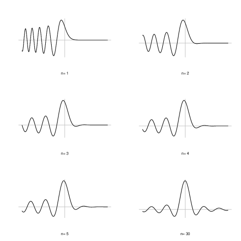
Figure 1. Profiles of odd-order solutions, $m=2n+1$

References

• Accetta and Orsingher [1997] G.Β Accetta and E.Β Orsingher. Asymptotic expansion of fundamental solutions of higher order heat equations. Random Oper. Stochastic Equations, 5:217 – 226, 1997.
• Beghin and Orsingher [2009] L.Β Beghin and E.Β Orsingher. Fractional Poisson processes and related random motions. Elect. J. Probab., 14:1790 – 1826, 2009.
• Bernstein [1919] F.Β Bernstein. Über das Fourierintegral $\int_{0}^{\infty}e^{-x^{4}}\cos tx\,dx$. Math. Ann., 79:265 – 258, 1919.
• Burwell [1923] W.Β R. Burwell. Asymptotic expansions of generalized hypergeometric functions. Proc. Lond. math. Soc., 22:57 – 72, 1923.
• Gradshteyn and Ryzhik [2007] I.Β S. Gradshteyn and I.Β M. Ryzhik. Table of integrals, series and products. Academic Press, 2007. Seventh edition.
• Lachal [2003] A.Β Lachal. Distributions of sojourn time, maximum and minimum for pseudo-processes governed by higher-order heat-type equations. Elect. J. Probab., 8(20):1 – 53, 2003.
• LΓ©vy [1923] P.Β LΓ©vy. Sur une application de la derivΓ©e d’ordre non entier au calcul des probabilitΓ©s. C.R. Acad. Sci., 179:1118–1120, 1923.
• Li and Wong [1993] X.Β Li and R.Β Wong. Asymptotic behaviour of the fundamental solution to $\partial u/\partial t=-(-\triangle)^{m}u$. Proceedings: Mathematical and Physical Sciences, 441(1912):423 – 432, 1993.
• Orsingher and Beghin [2009] E.Β Orsingher and L.Β Beghin. Fractional diffusion equations and processes with randomly varying time. Ann. Probab., 37:206 – 249, 2009.
• Orsingher and D’Ovidio [2011] E.Β Orsingher and M.Β D’Ovidio. Vibrations and fractional vibrations of rods, plates and Fresnel pseudo-processes. J. Stat. Phys., 145:143 – 174, 2011.
• PΓ²lya [1923] G.Β PΓ²lya. On the zeros of an integral function represented by Fourier’s integral. Messenger Math., 52:185 – 188, 1923.