RM3-TH/12-4

$S_{3}$ as a flavour symmetry for quarks and leptons after the Daya Bay result on $\theta_{13}$

Davide Meloni  

Dipartimento di Fisica ”E. Amaldi”

Universitá degli Studi Roma Tre, Via della Vasca Navale 84, 00146 Roma, Italy

We present a model based on the flavour group $S_{3}\times Z_{3}\times Z_{6}$ to explain the main features of fermion masses and mixing. In particular, in the neutrino sector the breaking of the $S_{3}$ symmetry is responsible for a naturally small $r=\Delta m^{2}_{sol}/\Delta m^{2}_{atm}$ and suitable next-to-leading order corrections bring $\theta_{13}$ at the level of $\sim 0.13$, fully compatible with the recent Daya Bay result. In the quark sector, the model accommodates the different mass hierarchies in the up and down quark sectors as well as the Cabibbo angle and $|V_{cb}|$ (or $|V_{ub}|$, depending on the charge assignment of the right-handed b-quark) in the correct range.

1 Introduction

One of major challenges in the model building is to provide a framework where the hierarchies in the fermion masses and the values of the mixing angles can be explained in a natural way. Recent results in the neutrino sector [1] have inspired many authors to discuss the possible origin of a relatively large reactor angle, as obtained first by the T2K and MINOS collaborations [2] and, more recently, by Double Chooz [3] and Daya Bay [4]. In particular, the latter has given a 5.2$\sigma$ evidence of $\theta_{13}\neq 0$:

$$\sin^{2}2\theta_{13}=0.092\pm 0.016\pm 0.005\,,$$ (1)

probably solving the longstanding question of the magnitude of $\theta_{13}$ (see [5],[6],[7], [8] and [9] for a discussion of the impact of such a result for lepton flavour mixing and leptonic CP violation). Several models based on the breaking of additional symmetries beyond the Standard Model have been proposed to explain this and other peculiarities emerged from neutrino oscillation experiments, as the large solar and atmospheric mixing angles as well as a small solar-to-atmospheric mass differences ratio $r$. In an unified view of fermion mass hierarchies and flavour mixing, the quark sector must also be taken into account and this poses the question of how to reconcile the numerous differences in the spectra and mixing of quarks compared to leptons, the most relevant ones being a different structure of the CKM mixing matrix and the strong mass hierarchy in the up-quark sector. Although many attempts have been done in this direction, the question of explaining the values of fermion masses and mixing (one of the aspects of the flavour problem) is still an open issue and deserves further studies. Discrete symmetries [10] have been invoked as a powerful tool to solve/mitigate some of these problems and, among several choices, the non-abelian discrete group $S_{3}$ [11] has also been investigated. Remarkably, models based on $S_{3}$ describing both quarks and leptons (with very few assumptions on the scalar and Yukawa sectors of the theory) are not very common. Interesting attempts in this direction have been done in the context of GUT theories [12] and in a non-unified approach [13]-[14]. In this paper we want to contribute to this discussion, presenting a SUSY see-saw model based on the flavour group $S_{3}\times Z_{3}\times Z_{6}$. Identifying $\varepsilon$ as the small $S_{3}$ breaking parameter (whose magnitude will be discussed later), the main features of our construction are:

• the neutrino mass hierarchy can only be of normal type;

• the solar-to-atmospheric mass differences ratio $r$ is naturally small, at the level of ${\cal O}(\varepsilon^{2})$, without invoking any fine-tuning among the Yukawa parameters (Sect.2);

• after the inclusion of suitable next-to-leading order corrections (NLO), the vanishing leading order (LO) $\theta_{13}$ receives a relatively large shift of ${\cal O}(\varepsilon)$ whereas $\theta_{23}$ is only modified by terms of ${\cal O}(\varepsilon^{2})$; the solar angle remains large, of ${\cal O}(1)$ (Sects.4-5);

• in the quark sector, we are able to reproduce the correct order of magnitude of the mass hierarchies in both up and down sectors (Sect.6);

• the Cabibbo angle is predicted in the correct range as well as $|V_{cb}|$ (or $|V_{ub}|$, depending on the charge assignment of the right-handed b-quark);

• the flavon alignments needed to get the previous results are obtained from the minimization of the superpotential allowed by the symmetry of the model (Sect.3).

A bit more problematic is the explanation of the muon-to-tau mass ratio and the value of $|V_{ub}|$ (or $|V_{cb}|$), in any case naturally smaller than the Cabibbo angle. Other interesting features of our model are the prediction for the effective mass $|m_{ee}|$, quite small as usual for neutrinos with normal mass ordering, and the fact that the Tri-bimaximal mixing structure (TBM) [15] can be easily obtained using only one additional relation among the Yukawas (not dictated by the symmetry of the theory).

The model is formulated in the framework of the SUSY see-saw mechanism. At LO, the contribution to $\theta_{12}$ only comes from the neutrino sector whereas $\theta_{23}$ is completely generated by the charged lepton sector. At this order, the reactor angle is vanishing. To produce such a pattern, the mass matrices $m_{\ell}\,m^{\dagger}_{\ell}$ and $m_{\nu}$ must be block-diagonal in the (23) and (12) sectors, respectively. In particular, having a block-diagonal light neutrino mass matrix helps in giving different order of magnitude to the mass eigenstates and then in obtaining a small $r$.

We use a non-conventional assignment of the left-handed doublets $L$ of the second and third generations in a 2 representation of $S_{3}$ as follows:

$$L=\left(\begin{array}[]{c}\tau\\ \mu\end{array}\right)\,,$$ (2)

whereas for the right-handed doublet we assume:

$$L^{c}=\left(\begin{array}[]{c}\mu^{c}\\ \tau^{c}\end{array}\right)\,.$$ (3)

Electron fields are assigned to the singlet $1$. In the neutrino sector, we introduce three right-handed fields: the first two generations are grouped in the 2 representation:

$$\nu^{c}=\left(\begin{array}[]{c}\nu_{e}^{c}\\ \nu_{\mu}^{c}\end{array}\right)\,.$$ (4)

whereas $\nu_{3}^{c}$ belongs to a $1_{2}$. We use the following representation of the $S_{3}$ group:

$$S^{2}=T^{3}=(ST)^{2}=1~{}.$$ (5)

In the so-called “T-diagonal“ basis we have:

$$S=\left(\begin{array}[]{cc}0&1\\ 1&0\end{array}\right)\qquad T=\left(\begin{array}[]{cc}\omega&0\\ 0&\omega^{2}\\ \end{array}\right),$$ (6)

with $\omega=e^{i2/3\pi}$. The tensor products involving pseudo-singlets are given by $1_{2}\times 1_{2}=1$ and $1_{2}\times 2=2$ while the product of two doublets is $2\times 2=2+1+1_{2}$ which, in terms of the components of the two doublets $A=(a_{1},a_{2})^{\rm T}$ and $B=(b_{1},b_{2})^{\rm T}$, are as follows:

$$a_{1}b_{2}+a_{2}b_{1}\in 1\qquad a_{1}b_{2}-a_{2}b_{1}\in 1_{2}\qquad\left(\begin{array}[]{c}{}a_{2}b_{2}\\ a_{1}b_{1}\\ \end{array}\right)\in 2\,.$$ (7)

To ensure the breaking of $S_{3}$ along appropriate directions in the flavour space, we need two doublet flavons $\phi$ and $\xi$ with the following vevs (derived from the minimization of the superpotential, see Sect.3):

$$\langle\phi\rangle=v_{\phi}\,\left(\begin{array}[]{c}1\\ 1\end{array}\right)\qquad\langle\xi\rangle=v_{\xi}\,\left(\begin{array}[]{c}0\\ 1\end{array}\right)\,;$$ (8)

two other scalar singlets $\chi\sim 1$ and $\chi^{\prime}\sim 1_{2}$ are also needed to guarantee appropriate non-vanishing entries in the fermion mass matrices; both singlets have non vanishing vevs:

$$\langle\chi\rangle=v_{\chi}\qquad\langle\chi^{\prime}\rangle=v_{\chi}^{\prime}\,.$$ (9)

The particle content and the transformation properties of leptons, electroweak Higgs doublets and flavons under $S_{3}\times Z_{3}\times Z_{6}$ are summarized in Tab.1.

Field	$\nu^{c}$	$\nu^{c}_{3}$	$L_{e}$	$L_{e}^{c}$	$L$	$L^{c}$	$h_{u,d}$	$\phi$	$\chi$	$\xi$	$\chi^{\prime}$	$\xi_{0}$	$\Delta_{0}$
$S_{3}$	$2$	$1_{2}$	$1$	$1$	$2$	$2$	$1$	$2$	$1$	$2$	$1_{2}$	1	$2$
$Z_{6}$	$\omega$	$\omega$	$1$	$\omega^{3}$	$\omega^{5}$	$\omega^{3}$	1	$\omega^{4}$	$\omega^{4}$	$\omega^{4}$	$\omega^{5}$	$\omega^{4}$	$\omega^{4}$
$Z_{3}$	1	1	$1$	$\omega$	1	$\omega^{2}$	1	$\omega$	$\omega$	$1$	$1$	1	$\omega$
$U(1)_{R}$	$1$	$1$	$1$	$1$	$1$	$1$	$0$	$0$	$0$	$0$	$0$	$2$	$2$

Table 1: Transformation properties of leptons, electroweak Higgs doublets and flavons under $S_{3}\times Z_{3}\times Z_{6}$ and $U(1)_{R}$ .

2 Leptons: leading order

2.1 Charged leptons

The leading order lagrangian in the left-right basis reads:

$${\cal L}_{cl}=x_{1}\,L\,L^{c}\,h_{d}\,\frac{\phi}{\Lambda}+x_{2}\,L\,L^{c}\,h_{d}\,\frac{\chi}{\Lambda}\,.$$ (10)

At this stage, there are no contributions to the electron entries (since $\chi^{\prime}$ has been assigned to the $1_{2}$ representation) and the electron mass is vanishing. In the $\mu-\tau$ subsector the mass matrix is as follows:

$$m_{\ell}=\frac{v_{d}}{\Lambda}\,\left(\begin{array}[]{cc}x_{2}v_{\chi}&x_{1}v_{\phi}\cr x_{1}v_{\phi}&x_{2}v_{\chi}\end{array}\right)\,,$$ (11)

where $v_{d}=\langle h_{d}\rangle$. The phases of the Yukawas $x_{1,2}$ can be rotated away, with no loss of generality. The charged lepton masses and the mixing matrix are then:

$$m_{\mu}=\frac{v_{d}}{\Lambda}\left|x_{1}v_{\phi}+x_{2}v_{\chi}\right|\qquad m_{\tau}=\frac{v_{d}}{\Lambda}\left|x_{1}v_{\phi}-x_{2}v_{\chi}\right|\,,$$ (12)

$$U_{\ell}=\frac{1}{\sqrt{2}}\,\left(\begin{array}[]{cc}1&-1\cr 1&1\end{array}\right)\,.$$ (13)

The question is how to realize a naturally small muon-to-tau mass ratio. In [16] it has been suggested to introduce a further symmetry under which $x_{1}=-x_{2}$ and $v_{\phi}=v_{\chi}$; however, as pointed out in [14], this additional symmetry does not commute with $S_{3}$ and the whole symmetry group is larger than the latter. Here we observe that for real flavon vevs (as assumed here) any couple of real $(x_{1},x_{2})$ determines a larger and a smaller eigenvalue, so a mass splitting is quite natural in this model. If we want to correctly reproduce the mu-to-tau mass ratio we have to fine-tune the Yukawa parameters; in particular, assuming $m_{\mu}/m_{\tau}\sim\lambda^{2}$ ($\lambda$ being the Cabibbo angle) we get:

$$x_{1}=-x_{2}\,(1+2\,\lambda^{2})+{\cal O}(\lambda^{4})\,,$$ (14)

(so that, as expected, the two Yukawas must be opposite in sign and almost equal in magnitude). We notice that, at this level, we do not need to specify a value of the ratios of the flavon vevs over the cut-off $\Lambda$.

2.2 Neutrinos

The first useful terms to generate a Dirac mass matrix are:

$${\cal L}_{D}=a\,L\,\nu^{c}\,h_{u}+b\,L_{e}\,\nu_{3}^{c}\,h_{u}\,\frac{\chi^{\prime}}{\Lambda}\,,$$ (15)

so that:

$$m_{D}=v_{u}\,\left(\begin{array}[]{ccc}0&0&b\,\frac{\chi^{\prime}}{\Lambda}\cr a&0&0\cr 0&a&0\end{array}\right)\,,$$ (16)

where $v_{u}=\langle h_{u}\rangle$. For the Majorana mass matrix we have:

$${\cal L}_{M}=\alpha\,\nu^{c}\,\nu^{c}\,\xi+\beta\,\nu^{c}\,\nu_{3}^{c}\,\xi+\gamma\,\nu^{c}\,\nu^{c}\,\frac{{\chi^{\prime}}^{2}}{\Lambda}+\delta\,\nu_{3}^{c}\,\nu_{3}^{c}\,\frac{{\chi^{\prime}}^{2}}{\Lambda}\,,$$ (17)

and:

$$m_{M}=\left(\begin{array}[]{ccc}0&\gamma\,\frac{v_{\chi}^{\prime\,2}}{\Lambda}&\beta\,v_{\xi}\cr\gamma\,\frac{v_{\chi}^{\prime\,2}}{\Lambda}&\alpha\,v_{\xi}&0\cr\beta\,v_{\xi}&0&\delta\,\frac{v_{\chi}^{\prime\,2}}{\Lambda}\end{array}\right)\,.$$ (18)

The first contribution to the heavy masses arise from the previous matrix with $v_{\chi}^{\prime}=0$ and are:

$$\alpha\,v_{\xi}\,,\;\pm\beta\,v_{\xi}\,.$$ (19)

The degeneracy is then lifted by taking into account the corrections from the $v_{\chi}^{\prime}$ terms. The light neutrino mass matrix is obtained from the see-saw formula:

$$m_{\nu}=-m_{D}\,m_{M}^{-1}\,m_{D}^{T}\,;$$ (20)

to make the following analytical evaluations more readable, we fix $a=1$ (but it will be considered as a free parameter in the numerical evaluations to follow) and assume an equal order of magnitude of the flavon vevs to the cut-off ratio $\frac{\langle\Phi\rangle}{\Lambda}=\frac{v_{\Phi}}{\Lambda}=\varepsilon$, that we take as a small parameter. At first order in $\varepsilon$ we get:

$$m_{\nu}=-\frac{v_{u}^{2}}{v_{\Phi}}\,\left(\begin{array}[]{ccc}0&\frac{b}{\beta}\,\varepsilon&0\cr\frac{b}{\beta}\,\varepsilon&-\frac{\delta}{\beta^{2}}\,\varepsilon&0\cr 0&0&\frac{1}{\alpha}\end{array}\right)\,.$$ (21)

All phases can be reabsorbed into a redefinition of the right-handed neutrino fields, so we deal with real parameters. We see that, at this order, we get a block-diagonal form of the light mass matrix, with the contribution to the (12) sector of ${\cal O}(\varepsilon)$ and the (33) element larger. The matrix $m_{\nu}$ is compatible with normal hierarchy only and the light masses (still at the first order in $\varepsilon$) are then given by:

$$|m_{1}| = \left(\frac{v_{u}^{2}}{v_{\Phi}}\right)\,\left[\frac{(4b^{2}\beta^{2}+\delta^{2})^{1/2}-\delta}{2\beta^{2}}\right]\,\varepsilon$$

$$|m_{2}| = \left(\frac{v_{u}^{2}}{v_{\Phi}}\right)\,\left[\frac{(4b^{2}\beta^{2}+\delta^{2})^{1/2}+\delta}{2\beta^{2}}\right]\,\varepsilon$$ (22)

$$|m_{3}| = \left(\frac{v_{u}^{2}}{v_{\Phi}}\right)\,\frac{1}{\alpha}$$

so that the solar and atmospheric mass differences read:

$$\Delta m^{2}_{sol} = \left(\frac{v_{u}^{2}}{v_{\Phi}}\right)^{2}\,\frac{\delta(4b^{2}\beta^{2}+\delta^{2})^{1/2}}{\beta^{4}}\,\varepsilon^{2}$$

$$\Delta m^{2}_{atm} = \left(\frac{v_{u}^{2}}{v_{\Phi}}\right)^{2}\,\,\frac{1}{\alpha^{2}}+{\cal O}(\varepsilon^{2})\,.$$

Taking $\alpha=1$, $\Delta m^{2}_{atm}=2.5\times 10^{-3}$ eV² and $v_{u}=100$ GeV, we estimate $v_{\Phi}\sim 2\times 10^{14}$ GeV, which is a common order of magnitude for the heavy neutrino masses. It is now easy to derive the ratio $r$:

$$r = \frac{\Delta m^{2}_{sol}}{\Delta m^{2}_{atm}}=\frac{\alpha^{2}\,\delta\,(4b^{2}\beta^{2}+\delta^{2})^{1/2}}{\beta^{4}}\,\varepsilon^{2}$$ (24)

which, for ${\cal O}(1)$ parameters, is naturally suppressed by $\varepsilon^{2}$. The value of $\varepsilon$ cannot be precisely determined at this stage; to recover the experimental value $r\sim 1/30$, $\varepsilon$ should be as small as the Cabibbo angle but a small numerical enhancement (suppression) of the coefficient $\frac{\alpha^{2}\,\delta\,(4b^{2}\beta^{2}+\delta^{2})^{1/2}}{\beta^{4}}$ can bring it to smaller (larger) values. The matrix in eq.(21) determines a non-vanishing solar angle: a straightforward computation gives:

$$\tan^{2}\theta_{12}=1-\frac{2\delta}{(4b^{2}\beta^{2}+\delta^{2})^{1/2}+\delta}\,,$$ (25)

so that it is generically of ${\cal O}(1)$. Summarizing, the whole neutrino mixing matrix at LO $U_{PMNS}=U_{\ell}^{\dagger}\,U_{\nu}$ has a vanishing reactor angle, maximal $\theta_{23}$ and large ${\cal O}(1)$ solar angle.

It is interesting to observe that, to reproduce the TBM value $\tan^{2}\theta_{12}=1/2$, one simply needs

$$\delta=\pm b\,\beta/\sqrt{2}\,,$$ (26)

which is still a number of ${\cal O}(1)$; in this respect, this external condition does not appear to be completely unnatural since it does not require any strong hierarchy among the model parameters. Another interesting possibility to get the TBM matrix from the $S_{3}$ symmetry has been proposed in [17] where, however, after the inclusion of the charged lepton corrections one of the two allowed $S_{3}$ invariant Yukawa couplings must be switched off by hand. Notice that a maximal value for $\theta_{12}$ in our model can only be obtained if $\delta=0$, which implies a vanishing $\Delta m^{2}_{sol}$.

3 Flavon alignment

The structure of the flavon vevs can be obtained minimizing the scalar superpotential in the limit of exact SUSY [18]. Within this approach, a continuous $U(1)_{R}$ symmetry is introduced, under which matter fields have $R=1$, while Higgses and flavon fields have $R=0$. Such a symmetry will be eventually broken down to the R-parity by small SUSY breaking effects which can be neglected in the first approximation. Since the superpotential must have $R=2$, we need to introduce two additional scalar fields, a doublet $\Delta_{0}$ and a singlet $\xi_{0}$, with $R=2$. Within these assumptions, the relevant part of the scalar potential of the model is given by the F-terms with:

$$V_{F}=\sum_{i}\left|\frac{\partial w}{\partial\varphi_{i}}\right|^{2}\,.$$ (27)

In the following, we parametrize the vevs as:

$$\langle\phi\rangle=v_{\phi}\,\left(\begin{array}[]{c}\phi_{1}\\ \phi_{2}\end{array}\right)\qquad\langle\xi\rangle=v_{\xi}\,\left(\begin{array}[]{c}\xi_{1}\\ \xi_{2}\end{array}\right)\qquad\langle\chi\rangle=v_{\chi}\qquad\langle\chi^{\prime}\rangle=v_{\chi}^{\prime}\,,$$ (28)

where $\phi_{1,2}$ and $\xi_{1,2}$ are adimensional quantities. At the leading order we have:

$$w_{d}=g_{1}\,\xi_{0}\,\xi^{2}+g_{2}\,\Delta_{0}\,\phi^{2}+g_{3}\,\Delta_{0}\,\phi\,\chi\,.$$ (29)

The condition for the minima are:

$$\frac{\partial w_{d}}{\Delta_{0}^{1}} = g_{2}\,v_{\phi}^{2}\,\phi_{1}^{2}+g_{3}\,v_{\phi}\,\phi_{2}\,v_{\chi}=0$$

$$\frac{\partial w_{d}}{\Delta_{0}^{2}} = g_{2}\,v_{\phi}^{2}\,\phi_{2}^{2}+g_{3}\,v_{\phi}\,\phi_{1}\,v_{\chi}=0$$ (30)

$$\frac{\partial w_{d}}{\xi_{0}} = \xi_{1}\,\xi_{2}=0\,.$$

The set of equations admit the solution:

$$\phi_{1}=\phi_{2}\qquad v_{\chi}=-\frac{g_{2}}{g_{3}}\,v_{\phi}\qquad\xi_{1}=0\,.$$ (31)

The relation among $v_{\xi}$ and $v_{\phi}$ allows us to assume a common order of magnitude for these vevs; on the other hand, the choice $\xi_{1}=0,\,\xi_{2}\neq 0$ is not restrictive since the other one, with $\xi_{1}\neq 0,\xi_{2}=0$ [14], can be obtained acting with the generator $S$ on it. At this stage, the flavon $\chi^{\prime}$ does not appear in the superpotential. However, the first corrections to $w_{d}$ involve $\chi^{\prime\,4}$ and read:

$$\delta w_{d}=g_{1}^{\prime}\,\xi_{0}\,\frac{\chi^{\prime\,4}}{\Lambda^{2}}\,.$$ (32)

Since it appears with the driving field $\xi_{0}$, this term can modify the vev of the $\xi$ flavon; assuming a perturbed structure like:

$$\langle\xi\rangle=v_{\xi}\,\left(\begin{array}[]{c}\xi_{1}^{\prime}\\ 1+\xi_{2}^{\prime}\end{array}\right)\,,$$ (33)

the minimizing equation (at the first order in the perturbations $\xi_{1,2}^{\prime}$) gives:

$$2\,g_{1}\,v_{\xi}^{2}\,\xi_{1}^{\prime}+g_{1}^{\prime}\,\left(\frac{v_{\chi^{\prime}}^{2}}{\Lambda}\right)^{2}=0\,.$$ (34)

Dividing this equation by $1/\Lambda^{2}$ and assuming, as usual, that $v_{\xi}/\Lambda\sim v_{\chi^{\prime}}/\Lambda\sim\varepsilon$, we can estimate $\xi_{1}^{\prime}\sim\varepsilon^{2}$ and also:

$$\frac{v_{\chi}^{\prime\,4}}{\Lambda^{2}}=-\frac{2\,g_{1}}{g_{1}^{\prime}}\,v_{\xi}^{2}\,\varepsilon^{2}.$$ (35)

The perturbation $\xi_{2}^{\prime}$ remains unspecified and we put it to zero. Summarizing:

$$\langle\xi\rangle=v_{\xi}\,\left(\begin{array}[]{c}\xi^{\prime}\,\varepsilon^{2}\\ 1\end{array}\right),\qquad v_{\chi}^{\prime}\sim v_{\xi}\,,$$ (36)

with $\xi^{\prime}$ a coefficient of ${\cal O}(1)$. For the other two flavons $\phi$ and $\chi$, the first useful corrections arise at the level of five-flavon insertion. The corrective terms are then of relative ${\cal O}(\varepsilon^{3})$ with respect to the leading order results and will be neglected in the following. Then, the NLO corrections to the mass matrices will be computed using the vev structures for $\phi$ and $\chi$ as given in eqs.(8)-(9).

4 Next to leading order corrections

It is important to check that the previous results on the mixing angles are not destroyed once the corrections to the lagrangians are taken into account.

4.1 Charged leptons

The most relevant corrections come from the term:

$$\delta{\cal L}_{cl}=x_{3}\,L_{e}\,L^{c}\,h_{d}\,\frac{\phi\chi^{\prime}}{\Lambda^{2}}\,,$$ (37)

which modifies the mass matrix as follows:

$$\delta m_{\ell}=v_{d}\,\left(\begin{array}[]{ccc}0&x_{3}\varepsilon^{2}&-x_{3}\varepsilon^{2}\cr 0&0&0\cr 0&0&0\end{array}\right)\,.$$ (38)

Still working with real parameters for simplicity, we see that the expression of the masses are not modified whereas the mixing matrix is now given by:

$$U_{\ell}=\left(\begin{array}[]{ccc}$\text{sign}$\left[(x_{1}-x_{2})\,x_{3}\right]&\frac{\sqrt{2}\,x_{3}}{x_{1}-x_{2}}\,\varepsilon&0\cr\left|\frac{x_{3}}{x_{1}-x_{2}}\right|\,\varepsilon&\frac{1}{\sqrt{2}}&-\frac{1}{\sqrt{2}}\cr-\left|\frac{x_{3}}{x_{1}-x_{2}}\right|\,\varepsilon&\frac{1}{\sqrt{2}}&\frac{1}{\sqrt{2}}\end{array}\right)\,.$$ (39)

Then, there are new contributions to the leptonic $\theta_{12}$ and $\theta_{13}$ but not to the atmospheric angle, since the $2-3$ sub-block still remains unchanged at this order. The electron mass is not generated at this order but only at the level of 5-flavon insertion, from the following two (non-vanishing) operators:

$$L_{e}\,L_{e}^{c}\,h_{d}\,\left\{\xi^{2}\,\phi^{2}\,\chi^{\prime},\;\xi^{2}\,\phi\,\chi\,\chi^{\prime}\right\}\,,$$

which give a contribution of ${\cal O}(\varepsilon^{5})$; reminding that $m_{\tau}\sim\varepsilon$, the electron-to-tau mass ratio is of ${\cal O}(\varepsilon^{4})$. Considering that this ratio should be some units of $10^{-4}$, we deduce that $\varepsilon$ cannot be too different from $\approx 0.13$. It is important to stress, however, that this value of $\varepsilon$ is merely indicative, as it can be enhanced or suppressed by a proper arrangement of the Yuwaka couplings. We will study more in details the magnitude of the breaking parameter in Sect.5. As it will be clear in the next section, $U_{\ell}$ will provide the largest corrections to the LO results.

4.2 Neutrinos

At the next level of approximation, the light neutrino mass matrix can be still evaluated using eq.(20) but expanded now at ${\cal O}(\varepsilon^{2})$ with flavon alignments as discussed in Sect.3. Here we want to comment that the filling of some of the vanishing entries in eq.(16) and (18) requires multiple-flavon insertions; for example, the elements (22), (23), (31) and (33) in $m_{D}$ are generated by operators with three flavons (like $L\,\nu^{c}\,\phi^{3}\,h_{u}$) and are then of ${\cal O}(\varepsilon^{3})$. All next-to-leading order Majorana operators are also of ${\cal O}(\varepsilon^{3})$ since they contain at least four flavons. Then, the main contributions to the LO vanishing matrix elements in eq.(18) come from the vev shift in eq.(36) and are of ${\cal O}(\varepsilon^{2})$. From these considerations is not difficult to understand that the NLO light neutrino mass matrix is given by (still using $a=1$):

$$m_{\nu}=-\frac{v_{u}^{2}}{v_{\Phi}}\,\left(\begin{array}[]{ccc}0&\frac{b}{\beta}\,\varepsilon&\frac{b\,\gamma}{\alpha\,\beta}\,\varepsilon^{2}\cr\frac{b}{\beta}\,\varepsilon&-\frac{\delta}{\beta^{2}}\,\varepsilon&\left(\frac{\xi^{\prime}\beta^{2}-\gamma\delta}{\alpha\beta^{2}}\right)\varepsilon^{2}\cr\frac{b\,\gamma}{\alpha\,\beta}\,\varepsilon^{2}&\left(\frac{\xi^{\prime}\beta^{2}-\gamma\delta}{\alpha\beta^{2}}\right)\varepsilon^{2}&\frac{1}{\alpha}\end{array}\right)\,.$$ (40)

The expression of the neutrino mixing matrix is quite cumbersome; we have found that all eigenvalues and eigenvectors are corrected by (intricate) ${\cal O}(\varepsilon^{2})$ terms. As previously stated, the charged lepton rotation $U_{\ell}$ gives the main corrections to the LO results for $\theta_{12}$ and $\theta_{13}$, whereas the atmospheric angle only receives ${\cal O}(\varepsilon^{2})$ corrections from the neutrino sector. The final results for the mixing angles are then:

$$\tan\theta_{12} = \tan\theta_{12}^{LO}+\frac{\sqrt{2}\,x_{3}\,(4b^{2}\beta^{2}+d^{2})^{1/2}}{(x_{1}-x_{2})\sqrt{2b^{2}\beta^{2}+\delta[\delta+(4b^{2}\beta^{2}+d^{2})^{1/2}]}}\,\varepsilon+{\cal O}(\varepsilon^{2})$$

$$\tan\theta_{23} = 1+{\cal O}(\varepsilon^{2})$$ (41)

$$\sin\theta_{13} = \left|\frac{x_{3}}{x_{1}-x_{2}}\right|\varepsilon+{\cal O}(\varepsilon^{2})\,.$$

As we can see, it is not difficult to reconcile our results with the experimental data, barring accidental cancellations; in fact, the NLO have preserved many good features of the LO results (large solar and atmospheric mixings) while producing a relatively large shift for $\theta_{13}\sim{\cal O}(\varepsilon)$.

4.3 Effective mass terms and $|m_{ee}|$

The previous results are not substantially modified by effective Weinberg operators. Up to four-flavon insertion, the lagrangian is as follows:

$${\cal L}_{w}=\frac{\alpha_{w}}{\Lambda_{LN}}\,L_{e}\,L_{e}\,h_{u}\,h_{u}+\frac{\beta_{w}}{\Lambda^{3}_{LN}}\,L\,L\,h_{u}\,h_{u}\,\xi^{2}+\frac{\gamma_{w}}{\Lambda^{4}_{LN}}\,L_{e}\,L\,h_{u}\,h_{u}\,\xi^{2}\,\chi^{\prime}\,,$$ (42)

where $\Lambda_{LN}$ is the lepton number breaking scale. The contributions to the neutrino mass matrix is then:

$$m_{w}=\frac{v_{u}^{2}}{\Lambda_{LN}}\,\left(\begin{array}[]{ccc}\alpha_{w}&-\gamma_{w}\,\frac{v_{\Phi}^{3}}{\Lambda_{LN}^{3}}&0\cr-\gamma_{w}\,\frac{v_{\Phi}^{3}}{\Lambda_{LN}^{3}}&0&0\cr 0&0&\beta_{w}\,\frac{v_{\Phi}^{2}}{\Lambda^{2}_{LN}}\end{array}\right)\,,$$ (43)

so we still have a block-diagonal form. In practise, the relevant contribution to $m_{\nu}$ is given by the first operator in ${\cal L}_{w}$, which fills the (11) vanishing entry in eq.(40) with a term of ${\cal O}(v_{u}^{2}/\Lambda_{LN})$. In the case $\Lambda_{LN}\sim\Lambda$, this term also contributes to eq.(22) and eq.(LABEL:solatmLO), changing the coefficients in front of the $\varepsilon$ parameter but not their order of magnitude. In the case $\Lambda_{LN}\gg\Lambda$, this term is negligible and the effective operators do not play any relevant role in the determination of the neutrino masses and mixings.

To evaluate the prediction of our model for the effective mass $m_{ee}$, we work in the basis where the charged leptons are diagonal and extract the (11) matrix element of the rotated neutrino mass matrix, that is:

$$|m_{ee}|=|U_{\ell}^{T}\,m_{\nu}\,U_{\ell}|_{11}\,.$$ (44)

We get:

$$|m_{ee}|=\sin^{2}\theta_{13}\,\left|\frac{[2\,\alpha\,b\,(x_{1}-x_{2})+\beta\,x_{3}]}{\alpha\,\beta\,x_{3}}\right|\,.$$ (45)

As expected in models for the normal hierarchy, $|m_{ee}|$ is small, at the level of $\theta_{13}^{2}$, although a clear correlation with the reactor angle is lacking because of the ${\cal O}(1)$ coefficient.

5 Numerical analysis of the lepton sector

The main purpose of this section is to analyze in detail the implication of our model for the lepton masses and mixing. In doing that, we use the NLO charged lepton and neutrino mass matrices as given in eqs.(11)-(38) and eq.(40) and perform a MonteCarlo simulation extracting complex lagrangian parameters with absolute values in the interval $[1/2,2]$ whereas the small $S_{3}$ breaking parameter is taken randomly in $[\lambda^{2},\lambda]$. To study more in detail the magnitude of $\varepsilon$, we imposed relaxed bounds on the charged lepton mass ratios:

$$2\times 10^{-3}<\frac{m_{e}}{m_{\mu}}<9\times 10^{-3}\qquad 2\times 10^{-2}<\frac{m_{\mu}}{m_{\tau}}<9\times 10^{-2}\,;$$ (46)

we also impose the constraints on the neutrino mass differences:

$$7.09\times 10^{-5}<\Delta m^{2}_{sol}<8.2\times 10^{-5}\,\text{eV}^{2}\qquad 2.14\times 10^{-3}<\Delta m^{2}_{atm}<2.76\times 10^{-3}\,\text{eV}^{2}\,,$$ (47)

derived from the second reference in [1], so that the value of $r$ is automatically reproduced. The main results of such an analysis are presented in Figs.1-2. In the former, we are interested to the dependence of $\sin^{2}\theta_{12}$ and $\sin^{2}\theta_{23}$ on the breaking scale $\varepsilon$.

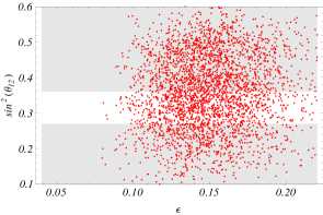
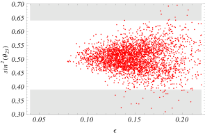
Figure 1: Mixing angles $\sin^{2}\theta_{12}$ (left panel) and $\sin^{2}\theta_{23}$ (right panel) as a function of the breaking scale $\varepsilon$. The horizontal gray bands are the regions excluded by the experimental data at 3$\sigma$, as obtained from the second reference in [1].

In these plots, the horizontal gray bands are the regions excluded by the experimental data at 3$\sigma$, as obtained from the second reference in [1]. We clearly see that $\varepsilon\sim{\cal O}(\lambda^{2})$ are almost excluded because too small to fill the relations in eq.(46). For every mixing angle, the bulk of the selected points is around $\varepsilon\sim 0.14$, not really different from the estimate we gave in Sect.4.1. The analytical results anticipated in eq.(41) are also confirmed; in particular, we see that the solar angle (left plot) is mainly undetermined but a large fraction of the points fall into the allowed 3$\sigma$ range, as a consequence of the fact that the TBM approximation is, in some sense, contained in the model via the simple relation in eq.(26). For the atmospheric angle (right plot), the majority of the points are well inside the 3$\sigma$ range, showing also a tendency to a largest spread for $\varepsilon\gtrsim 0.14$, as indicated in eq.(41). Similar considerations could also be drawn for the dependence of the reactor angle on $\varepsilon$; however, insted of presenting a scatter plot, we prefer to compare the $\sin^{2}2\theta_{13}$ distribution as obtained from our numerical simulation directly with the Daya Bay result. This is shown in Fig.2, where the 3$\sigma$ bounds derived from eq.(1) are enclosed in the solid vertical lines, whereas the dashed line is the best fit point. We can appreciate that, although the distribution is quite broad, the largest density of $\sin^{2}2\theta_{13}$ extractions is just inside the allowed region. We stress that this result has been obtained with an ab-initio simulation of the charged lepton and neutrino mass matrices with no other constraint than those given in eqs.(46-47). Notice that, given the large number of ${\cal O}(1)$ parameters, no definite predictions for the CP phase can be drawn.

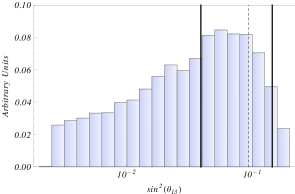
Figure 2: Distribution of the valus of $\sin^{2}2\theta_{13}$ as obtained from our model; the vertical solid lines enclose the 3$\sigma$ range derived from eq.(1) whereas the dashed line is the corresponding best fit point.

6 The quark sector

The $S_{3}\times Z_{3}\times Z_{6}$ symmetry provides a good description of the quark sector also; we use the same flavon fields and alignments described in the previous sections. The first two families of left-handed quarks are assigned to a $2$ representation of $S_{3}$ whereas all other fields belong to singles $1$ or $1_{2}$ in the case of $b^{c}$ (see Tab.2).

Field	$Q_{L}$	$q_{3_{L}}$	$u^{c}$	$c^{c}$	$t^{c}$	$b^{c}$	$s^{c}$	$d^{c}$
$S_{3}$	$2$	$1$	$1$	$1$	$1$	$1_{2}$	$1$	$1$
$Z_{6}$	$\omega^{5}$	$1$	$\omega^{4}$	$1$	$1$	$\omega$	1	$\omega^{4}$
$Z_{3}$	$\omega$	1	$1$	$\omega^{2}$	1	$1$	$\omega^{2}$	1

Table 2: Transformation properties of quarks under $S_{3}\times Z_{3}\times Z_{6}$.

The lagrangian in the up-quark sector, including all relevant operators to generate non-vanishing entries in the mass matrix, reads as follows:

$${\cal L}_{up} = a_{u}\,q_{3_{L}}\,h_{u}\,t^{c}+b_{u}\,q_{3_{L}}\,h_{u}\,c^{c}\,\frac{\xi^{2}\,\phi}{\Lambda^{3}}+c_{u}\,q_{3_{L}}\,h_{u}\,u^{c}\,\frac{\xi^{2}}{\Lambda^{2}}+d_{u}\,Q_{L}\,h_{u}\,t^{c}\,\frac{\phi^{2}\,\chi^{\prime}}{\Lambda^{3}}$$

$$+e_{u}\,Q_{L}\,h_{u}\,c^{c}\,\frac{\xi^{2}\,\chi^{\prime}}{\Lambda^{3}}+e_{u}^{\prime}\,Q_{L}\,h_{u}\,c^{c}\,\frac{\xi\,\chi^{\prime 3}}{\Lambda^{4}}+f_{u}\,Q_{L}\,h_{u}\,u^{c}\,\frac{(\xi^{2})_{2}\,(\phi^{2})_{2}\,\chi^{\prime}}{\Lambda^{5}}$$

$$+f_{u}^{\prime}\,Q_{L}\,h_{u}\,u^{c}\,\frac{(\xi^{2})_{2}\,(\phi^{2})_{1}\,\chi^{\prime}}{\Lambda^{5}}+f_{u}^{{}^{\prime\prime}}\,Q_{L}\,h_{u}\,u^{c}\,\frac{(\xi^{2})_{2}\,\phi\,\chi\,\chi^{\prime}}{\Lambda^{5}}+f_{u}^{{}^{\prime\prime\prime}}\,Q_{L}\,h_{u}\,u^{c}\,\frac{(\xi^{2})_{2}\,\chi^{2}\,\chi^{\prime}}{\Lambda^{5}}\,,$$

where we have indicated the $S_{3}$ contractions when necessary. The related mass matrix is as follows:

$$m_{up}=v_{u}\,\left(\begin{array}[]{ccc}(f_{u}+f_{u}^{{}^{\prime\prime}})\,\varepsilon^{5}&-e_{u}^{\prime}\,\varepsilon^{4}&-d_{u}\,\varepsilon^{3}\cr-(2f_{u}^{\prime}+f_{u}^{{}^{\prime\prime\prime}})\,\varepsilon^{5}&e_{u}\,\varepsilon^{3}&d_{u}\,\varepsilon^{3}\cr 2\,c_{u}\,\xi^{\prime}\,\varepsilon^{4}&b_{u}\,\varepsilon^{3}&a_{u}\end{array}\right)\,.$$ (52)

First of all, we observe that the mass hierarchy is well reproduced for the same value of $\varepsilon$ as deduced from the lepton sector; in particular, we have:

$$m_{u}=v_{u}\,(f_{u}+f_{u}^{{}^{\prime\prime}})\,\varepsilon^{5}\qquad m_{c}=v_{u}\,e_{u}\,\varepsilon^{3}\qquad m_{t}=v_{u}\,a_{u}\,.$$ (53)

Then, taking real Yukawas for simplicity, the matrix $U_{up}$ diagonalizing $m_{up}\,m_{up}^{\dagger}$ is given by:

$$U_{up}=\left(\begin{array}[]{ccc}1&\frac{e_{u}^{\prime}}{e_{u}}\,\varepsilon&\frac{d_{u}}{a_{u}}\,\varepsilon^{3}\cr-\frac{e_{u}^{\prime}}{e_{u}}\,\varepsilon&1&-\frac{d_{u}}{a_{u}}\,\varepsilon^{3}\cr-\frac{d_{u}}{a_{u}}\,\varepsilon^{3}&\frac{d_{u}}{a_{u}}\,\varepsilon^{3}&1\end{array}\right)\,.$$ (57)

This matrix goes into the desired direction: at LO, $U_{up}$ is the identity and at the NLO there exist a well defined hierarchy among the (12) element, not far away from the value of the Cabibbo angle, and the other off-diagonal matrix elements, which contribute to $V_{cb}$ and $V_{ub}$. From the charge assignment in Tab.2, we see that the operators in the down sector involving $d^{c}$ and $s^{c}$ are the same as those with $u^{c}$ and $c^{c}$, respectively (with the obvious replacement $h_{u}\to h_{d}$), whereas all operators including $b^{c}$ do not have a corresponding in ${\cal L}_{up}$; then we have:

$${\cal L}_{down} = a_{d}\,q_{3_{L}}\,h_{d}\,b^{c}\,\frac{\chi^{\prime}}{\Lambda}+b_{d}\,q_{3_{L}}\,h_{d}\,s^{c}\,\frac{\xi^{2}\,\phi}{\Lambda^{3}}+c_{d}\,q_{3_{L}}\,h_{d}\,d^{c}\,\frac{\xi^{2}}{\Lambda^{2}}+d_{d}\,Q_{L}\,h_{d}\,b^{c}\,\frac{(\phi^{2})_{1}\,\xi}{\Lambda^{3}}$$

$$+d_{d}^{\prime}\,Q_{L}\,h_{d}\,b^{c}\,\frac{(\phi^{2})_{2}\,\xi}{\Lambda^{3}}+d_{d}^{{}^{\prime\prime}}\,Q_{L}\,h_{d}\,b^{c}\,\frac{\chi^{2}\,\xi}{\Lambda^{3}}+d_{d}^{{}^{\prime\prime\prime}}\,Q_{L}\,h_{d}\,b^{c}\,\frac{\chi\,\phi\,\xi}{\Lambda^{3}}$$

$$+e_{d}\,Q_{L}\,h_{d}\,s^{c}\,\frac{\xi^{2}\,\chi^{\prime}}{\Lambda^{3}}+e_{d}^{\prime}\,Q_{L}\,h_{d}\,s^{c}\,\frac{\xi\,\chi^{\prime 3}}{\Lambda^{4}}+f_{d}\,Q_{L}\,h_{d}\,d^{c}\,\frac{(\xi^{2})_{2}\,(\phi^{2})_{2}\,\chi^{\prime}}{\Lambda^{5}}$$

$$+f_{d}^{\prime}\,Q_{L}\,h_{d}\,d^{c}\,\frac{(\xi^{2})_{2}\,(\phi^{2})_{1}\,\chi^{\prime}}{\Lambda^{5}}+f_{d}^{{}^{\prime\prime}}\,Q_{L}\,h_{d}\,d^{c}\,\frac{(\xi^{2})_{2}\,\phi\,\chi\,\chi^{\prime}}{\Lambda^{5}}+f_{d}^{{}^{\prime\prime\prime}}\,Q_{L}\,h_{d}\,d^{c}\,\frac{(\xi^{2})_{2}\,\chi^{2}\,\chi^{\prime}}{\Lambda^{5}}\,,$$

with mass matrix as:

$$m_{down}=v_{d}\,\varepsilon\,\left(\begin{array}[]{ccc}(f_{d}+f_{d}^{{}^{\prime\prime}})\,\varepsilon^{4}&-e_{d}^{\prime}\,\varepsilon^{3}&-(2d_{d}+d_{d}^{{}^{\prime\prime}})\,\varepsilon^{2}\cr-(2f_{d}^{\prime}+f_{d}^{{}^{\prime\prime\prime}})\,\varepsilon^{4}&e_{d}\,\varepsilon^{2}&(d_{d}^{\prime}+d_{d}^{{}^{\prime\prime\prime}})\,\varepsilon^{2}\cr 2\,c_{d}\,\xi^{\prime}\,\varepsilon^{3}&b_{d}\,\varepsilon^{2}&a_{d}\end{array}\right)\,.$$ (62)

Again, the mass ratios are well reproduced, since:

$$m_{d}=v_{d}\,(f_{d}+f_{d}^{{}^{\prime\prime}})\,\varepsilon^{5}\qquad m_{s}=v_{d}\,e_{d}\,\varepsilon^{3}\qquad m_{b}=v_{d}\,a_{d}\,\varepsilon\,.$$ (63)

Also, the bottom-to-top mass ratio is given by

$$\frac{m_{b}}{m_{t}}=\left(\frac{a_{d}}{a_{u}}\right)\,\varepsilon\,(\tan\beta)^{-1}\,,$$ (64)

implying $\tan\beta\sim 5$ for Yukawas of ${\cal O}(1)$. The matrix $U_{down}$ diagonalizing $m_{down}\,m_{down}^{\dagger}$ is given by:

$$U_{d}=\left(\begin{array}[]{ccc}1&\frac{e_{d}^{\prime}}{e_{d}}\,\varepsilon&(2d_{d}+d_{d}^{{}^{\prime\prime}})\,\varepsilon^{2}\cr-\frac{e_{d}^{\prime}}{e_{d}}\,\varepsilon&1&-(d_{d}^{\prime}+d_{d}^{{}^{\prime\prime\prime}})\,\varepsilon^{2}\cr-(2d_{d}+d_{d}^{{}^{\prime\prime}})\,\varepsilon^{2}&(d_{d}^{\prime}+d_{d}^{{}^{\prime\prime\prime}})\,\varepsilon^{2}&1\end{array}\right)\,.$$ (68)

Two comments are in order: on the one-hand, the $(12)$ element is still of the correct order of magnitude to explain, in combination with the result from the up sector, the value of the Cabibbo angle. On the other hand, all other off diagonal entries are smaller that $(12)$ but the (13) element is a bit larger than the required values to fit $V_{ub}$. In fact, these elements in eq.(68) are the dominant contributions to $V_{cb}$ and $V_{ub}$ in the CKM, since the corresponding matrix elements in eq.(57) are generally smaller. In fact, we get:

$$V_{us} = \left(\frac{e_{d}^{\prime}}{e_{d}}-\frac{e_{u}^{\prime}}{e_{u}}\right)\,\varepsilon\qquad V_{ub}=(2d_{d}+d_{d}^{{}^{\prime\prime}})\,\varepsilon^{2}\qquad V_{cb}=-(d_{d}^{\prime}+d_{d}^{{}^{\prime\prime\prime}})\,\varepsilon^{2}$$

$$V_{cd} = -V_{us}\qquad V_{td}=-V_{ub}\qquad V_{ts}=-V_{cb}\,.$$

Obviously, the last equalities are lifted once the ${\cal O}(\varepsilon^{3})$ terms are taken into account. To corroborate the previous considerations, we perform a numerical simulation of the up and down mass matrices of eqs.(52) and (62) extracting, as we did for the lepton sector, complex Yukawa parameters with absolute values in the interval $[1/2,2]$. We fixed the breaking scale $\varepsilon=0.15$, as suggested by the same procedure done in the lepton sector. We also impose the following constraints on the relevant mass ratios [19]:

$$5.40\times 10^{-6}<\frac{m_{u}}{m_{t}}<1.18\times 10^{-5} 3.60\times 10^{-3}<\frac{m_{c}}{m_{t}}<4.10\times 10^{-3}$$

$$7.90\times 10^{-4}<\frac{m_{d}}{m_{b}}<1.34\times 10^{-3} 1.60\times 10^{-2}<\frac{m_{s}}{m_{b}}<2.90\times 10^{-2}\,.$$

Our results for every CKM matrix elements are shown in fig.3, where we plot the absolute values of the nine distributions of the $V_{ij}$ entries. The diagonal entries are displayed in linear scale whereas we adopt a log scale for the off-diagonal elements; for them, we also showed the best fit values [20] with a solid vertical line.

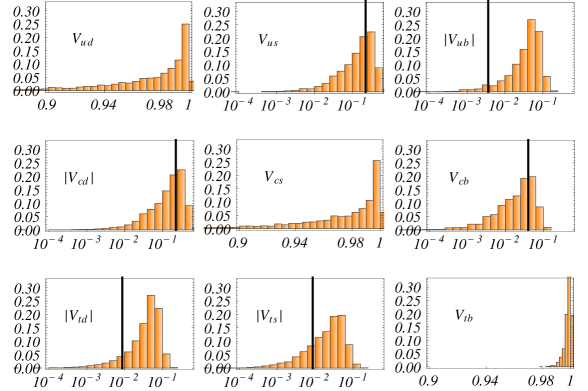
Figure 3: Distributions of the CKM matrix elements as obtained in our model. The best fit values [20] of the off-diagonal matrix elements are shown with a solid vertical line.

As we can see, it is very easy in our model to reproduce, with no fine-tuning, the correct values of $V_{us},V_{cd}$ as well as $V_{cb},V_{ts}$ while a small discrepancy remains with the best fit of $V_{ub}$ and $V_{td}$, as anticipated above. To make also these matrix elements fully compatible with the data, we need a moderate cancellation among the Yukawas $d_{d}^{\prime}$ and $d_{d}^{{}^{\prime\prime\prime}}$, see eq.(68). We do not present any plot related to the CP phase since the large number of ${\cal O}(1)$ parameters does not allow any definite prediction. As a last comment, we observe that taking a charge assignment for the field $b^{c}$ as the one adopted for $t^{c}$, we would get a structure of $U_{d}$ similar to $U_{up}$ as given is eq.(57); this automatically would imply $V_{ub}\sim V_{cb}\sim V_{td}\sim V_{ts}\sim\varepsilon^{3}$, so an enhancement should be invoked to reproduce the values of $V_{ub}$ and $V_{td}$. In this case, the bottom-to-tau mass ratio would be completely explained by large $\tan\beta$.

7 Conclusions

The Daya Bay Collaboration has released the measurement of the reactor angle $\theta_{13}$, showing a 5.2$\sigma$ discrepancy from zero. From the model building point of view, neutrino mass textures predicting a vanishing $\theta_{13}$ at leading order seem to be less appealing, unless large corrections bring the reactor angle to values compatible with the recent results, without destroying the predictions for the other mixing parameters. In this paper we have presented a see-saw SUSY model for fermion masses and mixing based on the non-abelian discrete symmetry $S_{3}$, whose main result is the prediction of a large $\theta_{13}\sim 0.13$, fully compatible with the Daya Bay claim of eq.(1). Other remarkable features of our construction are:

• in the lepton sector, the spectrum is of normal type, with $\theta_{12}$ and $\theta_{23}$ compatible with their experimental allowed ranges;

• in the quark sector, we obtained a good description of the relevant mass ratios and the absolute values of all the CKM matrix elements (including the Cabibbo angle) but $V_{ub},V_{td}$, for which we need a moderate fine-tuning among the Yukawas defining these matrix elements;

• the flavon alignments needed to get the previous results are natural minima of the superpotential in the SUSY limit.

References

• [1] G. L. Fogli, E. Lisi, A. Marrone, A. Palazzo and A. M. Rotunno, Phys. Rev. D 84, 053007 (2011) [arXiv:1106.6028 [hep-ph]]; T. Schwetz, M. Tortola and J. W. F. Valle, New J. Phys.  13, 109401 (2011) [arXiv:1108.1376 [hep-ph]].
• [2] K. Abe et al. [T2K Collaboration], Phys. Rev. Lett.  107, 041801 (2011) [arXiv:1106.2822 [hep-ex]]; L. Whitehead [MINOS Collaboration], ” Recent results from MINOS”
http://theory.fnal.gov/jetp/
• [3] Y. Abe et al. [DOUBLE-CHOOZ Collaboration], arXiv:1112.6353 [hep-ex].
• [4] F. P. An et al. [DAYA-BAY Collaboration], arXiv:1203.1669 [hep-ex]
• [5] Z. -z. Xing, arXiv:1203.1672 [hep-ph].
• [6] D. Meloni, S. Morisi and E. Peinado, arXiv:1203.2535 [hep-ph].
• [7] G. C. Branco, R. G. Felipe, F. R. Joaquim and H. Serodio, arXiv:1203.2646 [hep-ph].
• [8] X. Zhang and B. Q. Ma, arXiv:1203.2906 [hep-ph].
• [9] H. J. He and X. J. Xu, arXiv:1203.2908 [hep-ph].
• [10] G. Altarelli and F. Feruglio, Rev. Mod. Phys.  82, 2701 (2010) [arXiv:1002.0211 [hep-ph]].
• [11] N. Haba and K. Yoshioka, Nucl. Phys. B 739, 254 (2006) [hep-ph/0511108].
• [12] Y. Koide, Phys. Rev. D 69, 093001 (2004) [hep-ph/0312207]; S. Morisi and M. Picariello, Int. J. Theor. Phys.  45, 1267 (2006) [hep-ph/0505113]; R. N. Mohapatra, S. Nasri and H. -B. Yu, Phys. Lett. B 636, 114 (2006) [hep-ph/0603020].
• [13] S. -L. Chen, M. Frigerio and E. Ma, Phys. Rev. D 70, 073008 (2004) [Erratum-ibid. D 70, 079905 (2004)] [hep-ph/0404084]; Z. -z. Xing, D. Yang and S. Zhou, Phys. Lett. B 690, 304 (2010) [arXiv:1004.4234 [hep-ph]].
• [14] F. Feruglio and Y. Lin, Nucl. Phys. B 800, 77 (2008) [arXiv:0712.1528 [hep-ph]].
• [15] P. F. Harrison, D. H. Perkins and W. G. Scott, Phys. Lett. B 530, 167 (2002) [hep-ph/0202074].
• [16] W. Grimus and L. Lavoura, Phys. Lett.  B 572 (2003) 189 [arXiv:hep-ph/0305046]; W. Grimus and L. Lavoura, J. Phys. G 30 (2004) 73 [arXiv:hep-ph/0309050]; W. Grimus and L. Lavoura, JHEP 0508 (2005) 013 [arXiv:hep-ph/0504153].
• [17] R. N. Mohapatra, S. Nasri and H. -B. Yu, Phys. Lett. B 639, 318 (2006) [hep-ph/0605020].
• [18] G. Altarelli and F. Feruglio, Nucl. Phys. B 741, 215 (2006) [hep-ph/0512103].
• [19] K. Nakamura et al. (Particle Data Group), J. Phys. G 37 (2010) 075021.
• [20] http://www.utfit.org/UTfit/