EQUATION OF STATE FOR WATER IN THE SMALL COMPRESSIBILITY REGION

Abstract

The equation of state for dense fluids has been derived within the framework of the Sutherland and Katz potential models. The equation quantitatively agrees with experimental data on the isothermal compression of water under extrapolation into the high pressure region. It establishes an explicit relationship between the thermodynamic experimental data and the effective parameters of the molecular potential.

1 Introduction

Deriving the equation of state (EoS) for water in a wide range of pressures and temperatures remains a challenging open problem, especially in the high pressure region. In the recent papers [1,​ 2,​ 3,​ 4] devoted to the water EoS, this problem was solved by fitting multiparameter formulae with such a large number of adjustable parameters that it approaches the number of experimental points. These methods are not based on reliable statistical mechanic foundations, and the applicability of these EoS is restricted. If the functional form of the EoS and their parameters are applicable to other substance or solution is an open question.

In comparison with the majority of one-component liquids, water reveals many unusual properties in its normal and supercooled states. The analysis of the diffusion peak of the quasi-elastic incoherent neutron scattering and the kinematic shear viscosity of water has shown that the global H-bond network disintegrates into an ensemble of weakly interacting clusters: dimers, trimers, tetramers, etc. [5,​ 6,​ 7,​ 8,​ 9]. It was also shown [10] that the properties of water in the supercritical region are determined by the averaged spherically symmetric potential. Therefore, it is reasonable to use such well-known models as Lennard-Jones, Buckingham, Sutherland or Katz potentials for water in the high pressure region.

In this paper, we derive the EoS for a supercritical fluid within the framework of the Sutherland and Katz potentials. In our previous work [11], we used a new version of the thermodynamic perturbation theory (TPT) originally proposed by Sysoev [11]. The main feature of the proposed TPT is in the assumption that the functional form of the perturbed potential is identical to the potential of the reference system. Therefore, the deviation of the potential of the more compressed system from the potential of the less compressed system is considered as a perturbation. On this basis, the concept of a reference thermodynamic state has been developed. A functional expansion of the free energy gave the possibility to derive, at a certain choice of the parameter expansion, two EoS modifications within the framework of a realistic model and the ‘‘soft’’ sphere potential one. As was shown in [11], these EoS correctly described the isothermal compression for supercritical fluids of inert gases.

Following [11], we use the free energy perturbation expansion

$$F_{V}\left({V_{0}}\right)=F_{0}\left({V_{0}}\right)+\sum\limits_{i<j}{\int{d\bar{r}_{i}}}d\bar{r}\,\Delta e\left({\bar{r}_{ij}}\right)\,\frac{{\delta F\left({V_{0}}\right)}}{{\delta e\left({\bar{r}_{ij}}\right)}}+$$

$$+\frac{1}{{2!}}\sum\limits_{\scriptstyle i<j\hfill\atop\scriptstyle e<m\hfill}{\int{d\bar{r}_{i}}}d\bar{r}_{j}d\bar{r}_{l}d\bar{r}_{m}\,\Delta e\left({r_{ij}}\right)\,\Delta e\left({r_{lm}}\right)\times$$

$$\times\frac{{\delta^{2}F\left({V_{0}}\right)}}{{\delta e\left({r_{ij}}\right)\delta e\left({r_{lm}}\right)}},$$ (1)

where $\Delta e\left({r_{ij}}\right)=e\left({r_{ij}}\right)-e_{0}\left({r_{ij}}\right)=e^{-\frac{{\varphi\left({qr_{ij}}\right)}}{{kT}}}-e^{-\frac{{\varphi\left({r_{ij}}\right)}}{{kT}}}$, $\phi\left({qr_{ij}}\right)$ is the potential of the perturbed system, and $q$ is a scale factor, $\bar{r}\to q\bar{r},q=\sqrt[{}^{3}]{{\frac{V}{{V_{0}}}}}$.

Equation (1) can be transformed into the expression for pressure (the details are given in [11])

$$P-P_{0}=\frac{{NkT\Delta V}}{V}-$$

$$-\frac{{\rho_{0}^{2}V_{0}}}{{6V}}\int\limits_{V}{g_{2}\left(r\right)}\exp\left[{\beta\left({-\Phi\left({qr}\right)+\Phi\left(r\right)}\right)}\right]\,\frac{{d\Phi\left({qr}\right)}}{{dr}}rd\bar{r}+$$

$$+\frac{{\rho_{0}^{2}}}{6}\int\limits_{V}{g_{2}\left(r\right)}\frac{{d\Phi\left({qr}\right)}}{{dr}}rd\bar{r}.$$ (2)

This expression was obtained within the framework of a realistic potential model, that can be presented in the general form

$$\varphi\left(r\right)=\Phi\left(r\right)+\psi\left(r\right),$$ (3)

where $\Phi\left(r\right)$ is the repulsive part of the potential, and $\psi\left(r\right)$ is its attractive part.

2 The Equation of State within the Framework of Sutherland and Katz Potential Models

In the case of short-range potentials, the expression for the pressure can be rewritten in the form

$$P=\frac{{NkT}}{V}-\frac{{\rho_{0}^{2}V_{0}}}{{6V}}\int\limits_{V}{g_{2}\left(r\right)f\left(r\right)}\upsilon\left(r\right)d\bar{r}-$$

$$-\frac{{\rho_{0}^{2}V_{0}}}{{6V}}\int\limits_{V}{g_{2}\left(r\right)}\upsilon_{0}\left(r\right)d\bar{r},$$ (4)

where $f\left(r\right)=e^{{}^{\left[{\beta\left({-\varphi\left({qr}\right)-\varphi\left(r\right)}\right)}\right]}}-1$, $\upsilon\left(r\right)=-\bar{\nabla}\varphi\left({qr}\right)\bar{r}$ is the virial of intermolecular forces and $\upsilon_{0}\left(r\right)=-\bar{\nabla}\varphi\left({qr}\right)\bar{r}\left|{{}_{q=1}}\right.=-\bar{\nabla}\varphi\left(r\right)\bar{r}$ is the virial of intermolecular forces in the reference state. With regard for the expression for the pressure in the reference state

$$P_{0}=\frac{{NkT}}{{V_{0}}}-\frac{{\rho_{0}^{2}}}{6}\int\limits_{V}{g_{2}\left(r\right)}\upsilon_{0}\left(r\right)d\bar{r},$$ (5)

we rewrite relation (4) as

$$P=\frac{{V_{0}P{}_{0}}}{V}-\frac{{\rho_{0}^{2}V_{0}}}{{6V}}\int\limits_{V}{g_{2}\left(r\right)f\left(r\right)}\upsilon\left(r\right)d\bar{r}-$$

$$-\frac{{\rho_{0}^{2}V_{0}}}{{6V}}\int\limits_{V}{g_{2}\left(r\right)\Delta}\upsilon\left(r\right)d\bar{r}.$$ (6)

Equation (6) can be expressed in the terms of $\Pi=\frac{{P-P_{0}}}{{P_{0}}}$ or $\Delta=\frac{{V_{0}-V}}{{V_{0}}}$, using of the approximate quality $\frac{{V_{0}}}{V}\approx 1+\Delta$

$$\Pi=\Delta+\left({1+\Delta}\right)\left({L+K}\right),$$ (7)

where

$$L=-\frac{{\rho_{0}^{2}}}{{6P_{0}}}\int\limits_{V}{g_{2}\left(r\right)f\left(r\right)}\upsilon\left(r\right)d\bar{r},$$ (8)

$$K=-\frac{{\rho_{0}^{2}}}{{6P_{0}}}\int\limits_{V}{g_{2}\left(r\right)}\Delta\upsilon\left(r\right)d\bar{r}.$$ (9)

Now the problem of deriving the EoS reduces to the evaluation of integrals (8) and (9). First, we consider the Sutherland potential

$$\varphi\left(r\right)=\left\{{\begin{array}[]{ll}{\infty,}&{r<d_{0},}\\ {-cr^{-m},}&{r>d_{0},}\\ \end{array}}\right.$$ (10)

$d_{0}$ is the molecular diameter, and the potential well depth $\varepsilon$ is defined by $\varepsilon=\frac{c}{{d_{0}^{m}}}$. Then $\varphi\left({qr}\right)$ is written as

$$\varphi\left({qr}\right)=\left\{{\begin{array}[]{ll}{\infty,}&{r<d_{0},}\\ {-c\left({\frac{{V_{0}}}{V}}\right)^{m/3}r^{-m},}&{r>d_{0},}\\ \end{array}}\right.$$ (11)

where $d=\sqrt[3]{{\frac{{V_{0}}}{V}}}d_{0}$. We calculate the singular force $-\frac{{d\varphi\left(r\right)}}{{dr}}$ following [13] and obtain

$$\upsilon\left({\bar{r}}\right)=-kT\delta\left({r-d}\right)r+cm\left({\frac{{V_{0}}}{V}}\right)^{m/3}r^{-m}\Theta\left({r-d}\right),$$ (12)

$$\Delta\upsilon\left({\bar{r}}\right)=-kT\left[{\delta\left({r-d}\right)-\delta\left({r-d_{0}}\right)}\right]r+$$

$$+cmr^{-m}\left[{\left({\frac{{V_{0}}}{V}}\right)^{m/3}\Theta\left({r-d}\right)-\Theta\left({r-d_{0}}\right)}\right],$$ (13)

$\delta\left({r-d}\right)$ is the Dirac delta function and $\Theta\left({r-d}\right)$ is the Heaviside step function. The expression for $L$ takes the form

$$L=-\frac{{2\pi\rho_{0}^{2}}}{{3P_{0}}}\bigg{[}{-kTg_{2}\left(d\right)f\left({r\downarrow d}\right)d^{3}+}$$

$${+cm\left({\frac{{V_{0}}}{V}}\right)^{m/3}\int\limits_{d}^{\infty}{g_{2}\left(r\right)r^{-m+2}f\left(r\right)}dr}\bigg{]}$$ (14)

where $f\left({r\downarrow d}\right)=\mathop{\lim}\limits_{r\to d+0}f\left(r\right)$ [13]. The integral in (14) can be evaluated if we assume that $g_{2}\left(r\right)\approx e^{-\beta\varphi\left(r\right)}.$ Then, in view of $\frac{{V_{0}}}{V}\approx 1+\Delta,$ we have

$$cm\left({\frac{{V_{0}}}{V}}\right)^{m/3}\int\limits_{d}^{\infty}{g_{2}\left(r\right)r^{-m+2}f\left(r\right)}d=$$

$$=\left({-\beta}\right)^{(3-m)/m}c^{3/m}\left[{\left({\frac{{V_{0}}}{V}}\right)^{2m/3}\gamma\left({x,y}\right)-}\right.$$

$$\left.{-\left({\frac{{V_{0}}}{V}}\right)^{m/3}\gamma\left({x,y\left({\frac{V}{{V_{0}}}}\right)^{m/3}}\right)}\right].$$ (15)

Here, $\gamma\left({x,y}\right)$ is the upper incomplete gamma function with $x=\frac{{m-3}}{\beta}$, $y=-\frac{{\beta c}}{{d_{0}^{m}}}$. Using the same assumptions for integral (9), we obtain

$$K=\frac{{2\pi\rho_{0}^{2}}}{{3P_{0}}}\left[{kT\left[{g_{2}\left(d\right)d^{3}-g_{2}\left({r\downarrow d_{0}}\right)d^{3}}\right]-}\right.$$

$$-\left({-\beta}\right)^{(3-m)/m}c^{3/m}\times$$

$$\times\left.{\left[{\left({\frac{{V_{0}}}{V}}\right)^{2m/3}\gamma\left({x,y\left({\frac{V}{{V_{0}}}}\right)^{m/3}}\right)-\gamma\left({x,y}\right)}\right]}\right],$$ (16)

where $g_{2}\left({r\downarrow d_{0}}\right)=\mathop{\lim}\limits_{r\to d+0}g_{2}\left(r\right)$. Since the parameter $\Delta$ is small, we can expand $g_{2}\left(d\right)$ at a point $d_{0}$ in the Taylor series

$$g_{2}\left(d\right)\approx g_{2}\left({r\downarrow d_{0}}\right)\left[{1+C\left(T\right)\Delta}\right],$$ (17)

T a b l e  1. : The values of the EoS parameters

$T$, K	$300$	$350$	$400$	$450$	$500$	$550$
$B(T)$, MPa	$9.63$	$8.55$	$7.70$	$6.55$	$5.10$	$3.35$
$C(T)$	$2.76$	$2.65$	$2.59$	$2.45$	$2.39$	$2.10$
$A(T)$, K-1	$0.0042$	$0.0037$	$0.0032$	$0.0027$	$0.0024$	$0.002$

where $C(T)=\frac{{d_{0}}}{3}\frac{{\partial\ln g(r)}}{{\partial r}}\left|{{}_{r\to d_{0}+0}}\right.$ is the function of the reference state. Since, in the approximation $\Delta\ll 1,$ $f\left({r\downarrow d}\right)=\exp\left({\frac{{\beta cm\Delta}}{{3d_{0}^{m}}}}\right)-1$ and $\frac{\Delta}{\Pi}\ll 1,$ Eq. (7) in the case of small compressibility takes the form

$$P=P_{0}+\left[{B\left(T\right)+P_{0}}\right]\bigg{[}\left({e^{\frac{\Delta}{{A\left(T\right)T}}}\!\!-1}\right)\left[{1+\Delta\left({2+C\left(T\right)}\right)}\right]-$$

$$-\left({1+C\left(T\right)}\right)\Delta+2\left({1+C\left(T\right)}\right)\Delta^{2}\bigg{]}+\Gamma,$$ (18)

$\Gamma$ is the term which comprises the incomplete gamma function

$$\Gamma=\frac{{2\pi\rho_{0}^{2}}}{{3P_{0}}}\left[{\left({-\beta}\right)^{(3-m)/m}c^{3/m}\left[{\left({\frac{{V_{0}}}{V}}\right)^{2m/3}\!\!-1}\right]\gamma\left({x,y}\right)}\right].$$ (19)

For the Sutherland model, it is expressed in terms of the second virial coefficient ${B_{2}\left(T\right)}$

$$\Gamma=\frac{{kT\rho_{0}}}{{P_{0}}}\left[{\left({\frac{{V_{0}}}{V}}\right)^{2m/3}-1}\right]\left[{B_{2}\left(T\right)+\frac{{2\pi d_{0}^{3}}}{3}}\right].$$ (20)

However, the analysis of the experimental data for some dense fluids (water, argon, neon, krypton) revealed that this term can be neglected under the condition $\Pi\approx 10^{3}$ with an accuracy of 1%. It is the fairly wide range of thermodynamic variables, where the isothermal compressibility is low ($\Delta\ll 1$) corresponding to the pressure interval 100–2200 MPa. The terms $2\left({1+C\left(T\right)}\right)\Delta^{2}-\left({1+C\left(T\right)}\right)\Delta$ can also be ignored with the same accuracy. Finally, we arrive at the EoS within the framework of the Sutherland model

$$P=P_{0}+\left[{B\left(T\right)+P_{0}}\right]\,\left[{\left({e^{\frac{\Delta}{{A\left(T\right)\,T}}}-1}\right)\,D\left(T\right)}\right],$$ (21)

where $D\left(T\right)=1+\Delta\left({2+C\left(T\right)}\right)$. Expression (21) is a three-constant equation of state with the adjustable parameters $B(T)$, $D(T),$ and $A(T)$ (see Table 1). The parameter $B(T)$ depends on the temperature. It is related to the pressure caused by attractive forces

$$B\left(T\right)=\frac{{2\pi\rho_{0}^{2}}}{{3_{0}}}kTg_{2}\left({r\downarrow d_{0}}\right)d_{0}^{3}-P_{0}=$$

$$=P_{0}^{r}-P_{0}=P_{0}^{a}-\frac{{NkT}}{{V_{0}}},$$ (22)

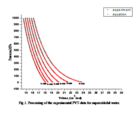
Fig. 1.: Processing of the experimental PVT-data for supercritical water

where $P_{0}^{r}$ is the pressure caused by the repulsive forces in the reference state, and $P_{0}^{a}$ is a part of the pressure due to the attractive forces. The parameter $A(T)$, within the framework of the Sutherland model, is expressed by the formula

$$A(T)=\frac{{3\,d_{0}^{m}\,k}}{{mc}}.$$ (23)

If we use the Katz potential model

$$\Phi\left({\bar{r}}\right)=\left\{{\begin{array}[]{ll}{\infty,}&{r<d_{0},}\\ {-\frac{{aR_{0}^{3}}}{{4\pi}}e^{-rR_{0}},}&{r>d_{0},}\\ \end{array}}\right.$$ (24)

where $R_{0}$ is the interaction radius of the attractive forces, $\frac{{aR_{0}^{3}}}{{4\pi}}$ is the interaction constant, Eq.(21) retains its functional form, but the parameter $A(T)$ is defined by the formula $A(T)=\frac{{12\,\pi d_{0}^{m}\exp\left({R_{0}d_{0}}\right)\,k}}{{d_{0}R_{0}^{4}a}}$.

The parameters $B(T)$ and $C(T)$ are defined in a similar way.

3 Experimental PVT-data Analysis

We used the technique from the previous paper [11] to process the PVT data and evaluate the EoS parameters. It turns out that Eq. (21) yields good agreement with the experimental PVT data [14] under the extrapolation to the high pressure region. The results of the comparison are presented in Figure.

Of special interest are the values of the parameter $A(T),$ because it is related to the parameters of the potential, formulae (23) and (25) for the Sutherland and Katz models. On the basis of (23), we evaluated the values of the potential well depth $\varepsilon$ at a fixed value $m=12$ commonly used in the Lennard–Jones model (Table 2).

T a b l e  2. : The values of $\varepsilon$ (Sutherland potential) at $m=12$ in the temperature interval 300–550 K

$T$, K	$300$	$350$	$400$	$450$	$500$	$550$
$\varepsilon$, $J10^{3}$/mole	$0.493$	$0.562$	$0.650$	$0.769$	$0.866$	$1.038$

If we fix the value of $\varepsilon=0.650$ kJ/mole, which corresponds to the SPC/E model, we obtain a variation of the softness parameter $m$ with the temperature. In general, fixing $\varepsilon$ at the values for well-known potential models such as SPC/Fw [15], TIP3P/Fw [15], and TIP5P/Ew [16] leads to a variation of the softness parameter $m$ with the temperature within the framework of the Sutherland potential.

4 Conclusion

The approach developed on the basis of the free energy perturbation expansion and a new version of TPT resulted in some universality for the EOS statistical foundation of the low weight molecular supercritical fluids. In principle, the concept of the thermodynamic reference state implies that an initial state ($P_{0}$, $V_{0}$) on the isotherm corresponds to the reference system with the unperturbed potential, and every subsequent point on the isotherm ($P_{1}$, $V_{2}$), …, ($P_{n}$, $V_{n}$) corresponds to the system with the perturbed potential at the isothermal compression of the system. This modification of TPT allowed obtaining the EoS which exhibits good results under the extrapolation to the high-pressure region and, most importantly, establishes a relationship between the parameters of the model potential and the thermodynamic properties of substances. This relationship gives estimations for the values of the parameter $\varepsilon$ (Table 2). Interestingly, the values are of the same order of magnitude as the values of many well-known water models (SPC/E, SPC/Fw, TIP3P/Fw, TIP5P/Ew). However, the temperature dependence of $\varepsilon$ in this region of thermodynamic variables indicates that the form of the Sutherland model is unsuitable for this high pressure region. Nevertheless, these data can be used as additional information for calibrating the potential parameters in simulations.

РIВНЯННЯ СТАНУ ВОДИ В ОБЛАСТI МАЛИХ
СТИСЛИВОСТЕЙ
В.Ю. Бардiк, Д.А. Нерух, Є.В. Павлов, I.В. Жиганюк
Р е з ю м е
Одержано статистично обґрунтоване рiвняння стану густих флюїдiв у рамках моделей потенцiалу Сюзерленда та Каца. Запропоноване рiвняння стану з високою точнiстю узгоджується з експериментальними даними по iзотермiчному стисненню води при екстраполяцiї в область високих тискiв. Встановлено кiлькiсний зв’язок мiж ефективними параметрами модельних потенцiалiв з параметрами рiвняння стану.

References

• [1] A. Saul and W. Wagner, J. Phys. Chem. Ref. Data 18, 1537 (1989).
• [2] W. Wagner and A. Pruss, J. Phys. Chem. Ref. Data 31, 387 (2002).
• [3] R.I. Nigmatulin and R.Kh. Bolotnova, Teplofiz. Vys. Temp. 46, 182 (2008).
• [4] R.I. Nigmatulin and R.Kh. Bolotnova, Teplofiz. Vys. Temp. 46, 325 (2008).
• [5] A.I. Fisenko and N.P. Malomuzh, Int. J. Mol. Sc. 10, 2383 (2009).
• [6] A.I. Fisenko and N.P. Malomuzh, Chem. Phys. 345, 164 (2008).
• [7] L.A. Bulavin, A.I. Fisenko, and N.P. Malomuzh, Chem. Phys. Lett. 453, 183 (2008).
• [8] A.I. Fisenko, N.P. Malomuzh, and A.V. Oleynik, Chem. Phys. Lett. 450, 297 (2008).
• [9] T.V. Lokotosh, N.P. Malomuzh, and K.N. Pankratov, J. Chem. Eng. Data 55, 2021 (2010).
• [10] S.V. Lishchuk, N.P. Malomuzh, and P.V. Makhlaichuk, Phys. Lett. A 374, 2084 (2010).
• [11] V.Yu. Bardik, N.P. Malomuzh, K.S. Shakun, and V.M. Sysoev, Journal of Molecular Liquids, in press.
• [12] V.M. Sysoev, Teor. Mat Fiz. 55, 305 (1983).
• [13] R. Reijnhart, Physica A 83, 533 (1976).
• [14] NIST Database http://webbook.nist.gov/chemistry/fluid/.
• [15] Y. Wu, H.L. Tepper, G.A. Voth, J. Chem. Phys. 124, 024503 (2006).
• [16] S.W. Rick, J. Chem. Phys. 120, 6085 (2004).
Received 17.05.11