Wall Orientation and Shear Stress in the Lattice Boltzmann Model

Abstract

The wall shear stress is a quantity of profound importance for clinical diagnosis of artery diseases. The lattice Boltzmann is an easily parallelizable numerical method of solving the flow problems, but it suffers from errors of the velocity field near the boundaries which leads to errors in the wall shear stress and normal vectors computed from the velocity. In this work we present a simple formula to calculate the wall shear stress in the lattice Boltzmann model and propose to compute wall normals, which are necessary to compute the wall shear stress, by taking the weighted mean over boundary facets lying in a vicinity of a wall element. We carry out several tests and observe an increase of accuracy of computed normal vectors over other methods in two and three dimensions. Using the scheme we compute the wall shear stress in an inclined and bent channel fluid flow and show a minor influence of the normal on the numerical error, implying that that the main error arises due to a corrupted velocity field near the staircase boundary. Finally, we calculate the wall shear stress in the human abdominal aorta in steady conditions using our method and compare the results with a standard finite volume solver and experimental data available in the literature. Applications of our ideas in a simplified protocol for data preprocessing in medical applications are discussed.

1 Introduction

Computer simulations of the blood flow in the human circular system allow physicians to visualize the internal flow structure, a capability that might have a significant impact on diagnosis and medical treatment of arterial diseases (for review see [1, 2, 3]). Digital simulations have been applied in many scenarios and for various purposes e.g. to study the role of hemodynamic forces in the development of atheromatous plaques in human cartoids atherosclerosis [4], in a clinical study on the rupture risk assesment in the cerebral aneurysm [5] or in a discovery of a shear-driven mechanism of platelet aggregation in arterial thrombosis [6]. Direct results of hydrodynamical simulations (velocity and pressure fields) are not practical in medical analysis. To better understand the impact of the blood flow dynamics on the complex biochemical phenomena associated with the development of vascular diseases, a wall shear stress (WSS, see Fig. 1) with its gradient (WSSG), a hoop stress or an oscillatory shear index (OSI) are often computed. WSS is a tangential force exerted on the unit of the wall surface by the flow [7] and OSI describes its deviation from the average direction [8]. WSS has been a subject of intensive research for many years, including studies on its role in development of human atherosclerosis [9, 10], the growth of an intracranial aneurysm [11] and development of the dissecting aneurysm in the human aorta [12]. WSS determines the structure, function and gene expression of an endothelial cells [4, 13]. It is now well established that a low shear stress is correlated with rapid development of various vascular malfunctions [14, 15, 16, 17, 18]. These facts motivate physicians to find applications of the WSS in diagnosis [19, 20] and to seek efficient and practical protocols for its measurement.

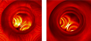
Figure 1: (color online) Wall shear stress magnitude in the bifurcation of the human abdominal aorta (the lighter color the higher the stress) calculated using a lattice Boltzmann model (left) and the finite volume method (right).

In order to compute WSS for patient-specific data one has to acquire the organ geometry, convert and import it to the Navier–Stokes solver, compute the velocity field and take gradients of its components at the wall. The process may be iterative and further time-averaging might be necessary if the flow is transient. The major difficulty of this procedure is the prohibitively long pre-processing and computation time which limits its applicability in a real patient diagnosis. The pre-processing involves mainly the conversion of digital data from the computer tomography scans into a three-dimensional mesh required by standard finite element/finite volume solvers [21, 22, 23]. High quality of the output mesh is required by flow solvers to work properly and computer-human interaction during the meshing process is often necessary. The flow solver runtime depends on many factors e.g. solver type, mesh resolution, flow properties and hardware used. It may be a bottleneck of the whole procedure as well, particularly for geometries of high resolution, time dependent flows and problems involving fluid-structure interaction. It is widely believed that the run time of fluid solvers could be significantly reduced by using efficient parallel algorithms on massively parallel architectures, e.g. graphics processing units (GPUs) [24].

Time issues mentioned above might be addressed with the lattice Boltzmann method (LBM), a recently developed method for solving fluid flow problems which is based on the kinetic theory of gases [25]. The method operates directly on voxel data and thus does not require meshing at the level of accuracy required by standard solvers. It also proved excellent parallel scalability on supercomputers [26, 27] as well as on emerging parallel architectures [28, 29, 30, 31]. The method was validated against analytical solutions in a two-dimensional oscillatory channel flow and its second order accuracy in space and time was confirmed [32, 33]. In medical applications, LBM was tested in solving time-dependend three-dimensional flows in models of the human abdominal aorta [34] and compared against finite element solvers in the superior mesentric artery blood flow [35]. Non-Newtonian LBM models also exist e.g. the Carreau–Yasuda fluid model applied in cerebral aneurysm problem [36]. Palabos, a parallel open source LBM implementation, was used to model blood flow in cerebral aneurysm and compared to a finite volume flow solver [37, 38] and the difference between the velocity fields obtained in both methods was estimated to be around 10$\%$. Application of LBM to modeling aneurysm and tumor development were recently discussed [39]. He et al. compared LBM combined with the level-set method to an OpenFOAM solver in patient-specific geometry [40].

Despite the second order accuracy of the LBM stress tensor in bulk fluid being recently reported [41, 42], the WSS in LBM suffers from inaccuracy introduced by a staircase boundary. The problem may be eased with subgrid boundary conditions [43] or the recently developed unstructured mesh LBM formulation [44], but both of them introduce additional complexity into the solver code, making it more difficult to maintain and parallelize. Recently Stahl et al. showed that a few lattice nodes away from the wall the error is significantly decreased in the standard LBM formulation [45]. He suggests to calculate normal vectors required by this procedure from the velocity field as the fluid flowing along the noslip walls follows its geometry. Thus, the normal at the boundary is approximated by the normal to the local velocity vector in a cell close to the wall. However, this method behaves peculiarly bad in a vicinity of the wall, with maximum error close to 90%. Moreover, it is not suitable for time dependent flow problems unless one solves an additional steady flow case. It also requires a solution to the eigenvalue problem and does not provide the vector sense relative to the wall.

In this paper we discuss another way of computing the normal vectors which does not suffer from above issues. If we look at the LBM staircase wall, we intuitively see its orientation. This is because we subconsciously average the input of all faces we see. A similar example is our brain’s handling of a two-dimensional line on a computer display: if pixels are small enough, the line orientation is easily recognized by eye. We propose to utilize similar averaging of a few boundary facets around the point of interest to compute the normal vectors required for evaluating WSS. The procedure is simple and its implementation consists of only a few algebraic operations. Therefore, no eigenvalue problem has to be solved. Additionally, the information about the normal sense is provided, and we show that our procedure tends to provide more accurate results. Henceforth the normals calculated in this way will be called ‘geometric normals’ and the normals approximated from the velocity field will be called ‘dynamic normals’.

The structure of the paper is as follows. In Sec. 2 and 3 we briefly introduce the lattice Boltzmann method and the formula for the wall shear stress. In Sec. 3.1 we explain how to compute geometric normals and verify them in simple geometries. The wall shear stresses in an inclined and a bent channel flow are calculated in Sec. 4. A comparison of WSS obtained with the lattice Boltzmann and a finite volume methods in the human abdominal aorta is given in Sec. 5. Section 6 presents the discussion of the results and Sec. 7 is devoted to conclusions.

2 The lattice Boltzmann method

LBM is a computational method of solving the Navier–Stokes equations. It was developed mainly as a remedy to noise issues of the lattice gas automata (LGA) [46, 47]. In LGA the local state of the system is described by a boolean variable $c_{\mathrm{i}}$, where $i$ runs over lattice vectors (vectors that link neighbour sites in the lattice). In contrast, LBM replaces $c_{\mathrm{i}}$ by a particle distribution function $f_{\mathrm{i}}\in[0,1]$, which is interpreted as the probability that a particle found in the lattice node moves along the $i$-th direction. A typical LBM algorithm runs two steps, propagation and collision, and is expressed by a set of discrete equations:

$$f_{\mathrm{\alpha}}(\mathbf{x}+\mathbf{c}_{\mathrm{\alpha}}\delta t,t+\delta t)=f_{\mathrm{\alpha}}(\mathbf{x},t)+\Omega_{\alpha}(\mathbf{f}),$$ (1)

where $\mathbf{c}_{\alpha}$ is the $\alpha$-th lattice vector, $\delta t$ is the time interval (usually $\delta t=1$) and $\Omega_{\alpha}(\mathbf{f})$ is a collision operator. The collision operator may realize either a linear relaxation to the equilibrium distribution function or the multirelaxation of separate hydrodynamical and kinetic moments [48]. The Chapman-Enskog analysis cane be used to show that the model reproduces incompressible Navier–Stokes equations [49].

As an implementation of LBM we used the Sailfish library [50]. Sailfish works on GPU processors. It is written in Python and utilizes template-based methodology for automatic device code generation on CUDA and OpenCL GPU platforms. The original code is freely available under the LGPL licence.

3 The wall shear stress

When fluid flows over a rigid surface, the velocity at the wall vanishes and the no slip boundary condition holds. However, in a vicinity of the wall the tangential component of the velocity does not vanish; the corresponding gradient of the tangential velocity component along the wall normal generates the wall shear stress, a force that is exerted by the fluid on the wall’s surface. WSS may be expressed as the difference between the Cauchy stress on a plane and its projection on the plane normal (see A). For an incompressible, Newtonian fluid the WSS in the lattice Boltzmann method can be calculated in terms of the non-equilibrium distribution function $f_{\alpha}^{neq}$:

$$\tau_{i}=\frac{\mu\omega}{c_{s}^{2}\varrho}f_{\alpha}^{neq}c_{\alpha j}n_{j}\left(c_{\alpha i}-c_{\alpha k}n_{i}n_{k}\right),$$ (2)

where $c_{s}$ is the lattice sound speed, $\mu$ is the dynamic viscosity, $\varrho$ is the fluid density, and $\omega$ is the LBM relaxation parameter. $c_{\alpha x}$ and $n_{x}$ denote lattice and normal vector components, i.e. $n_{i}$ is the $i$-th component of the wall normal vector $\mathbf{n}$ and $c_{\alpha i}$ is the $i$-th component of the lattice vector $\mathbf{c}_{\alpha}$. Einstein summation convention is implied. A detailed derivation of Eq. 2 is given in A with its algorithmic form in B.

3.1 Wall orientation

To calculate WSS with Eq. (2) the wall orientation and the corresponding wall normal $\mathbf{n}$ must be known. A typical three-dimensional LBM simulation works on a discrete, uniform grid built of adjacent cubic cells. If a fluid node has a no-slip boundary neighbour then there is a boundary facet between them at which the no-slip condition of zero velocity is fulfilled. The facet is perpendicular to the line that joins node centers whereas its physical location depends on the LBM relaxation time. For a three-dimensional model there are six possible boundary normals: $\pm\mathbf{e_{x}}=(\pm 1,0,0)$, $\pm\mathbf{e_{y}}=(0,\pm 1,0)$, and $\pm\mathbf{e_{z}}=(0,0,\pm 1)$.

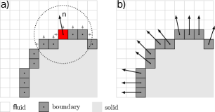
Figure 2: (color online) (left) A geometric normal vector (long arrow denoted as $\mathbf{n}$) is calculated by averaging input from normals of neighbouring fluid/no-slip boundary nodes (short arrows). Right: normal vectors computed for each individual boundary node. Geometric normals are enlarged for easier viewing.

In order to calculate $\mathbf{n}$ we suggest taking an average of normal vectors of the individual fluid/no-slip boundary facets in a spherical vicinity of the cell. For this we find all boundary facets whose centers lay in the sphere of radius $r$ centered at a given cell (Fig. 2a). If $\mathbf{b}_{i}$ is the boundary normal of the $i$-th facet then the above procedure may be expressed as the arithmetic mean:

$$\mathbf{n}=n_{b}^{-1}\sum_{i=0}^{n_{b}-1}\mathbf{b}_{i},$$ (3)

where $n_{b}$ is the number of facets within the neighborhood. The same procedure is repeated for each boundary cell (Fig. 2, right)

3.2 Weighted scheme

In the application of Eq. (3) an unacceptable averaging of normals that belong to separate or opposite fragments of the object’s surface may take place if $r$ is taken to be too large. In the hemodynamical scenario, this may occur in small arteries or bifurcation regions where object radii are smaller that $r$ and details may be lost due to averaging normals to opposite facets. Moreover, if $r$ is too small, $\mathbf{n}$ is influenced by the staircase approximation of the surface and may change rapidly from node to node. To deal with these issues we suggest to weight the mean in Eq. (3):

$$\mathbf{n}=\left(\sum_{i}w_{i}\right)^{-1}\sum_{i}w_{i}\mathbf{b}_{i},$$ (4)

where the sum goes over neighour facets. We choose $w_{i}=1/(1+d_{i})^{\gamma}$, where $d_{i}$ is the distance between the center of the node for which the average is computed and the center of the node with normal $\mathbf{b}_{i}$.

The exponent $\gamma$ defines how strongly concentrated the weighting is, with $\gamma=0$ corresponding to uniform weights (reducing to Eq. (3)); the strength of weighting increases with the value of $\gamma$.

3.3 Numerical tests for normal vectors

We test the above procedure in three-dimensional ball and tube geometries for which exact normal vectors are known. First, a boolean array of size $L^{3}$ is generated such that it holds $0$ if the voxel (three dimensional pixel) center lays inside the object and $1$ otherwise. Boundary cells are represented by voxels equal to $1$ having at least one adjacent zero neighbour. The object (ball or tube) radius is $R=L/2$ and we test three resolutions: $L=25^{3},50^{3}$ and $100^{3}$.

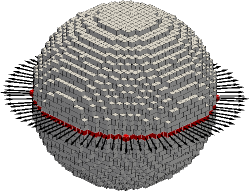
Figure 3: (color online) Geometry of the ball for L=25 (lattice units). Normal vectors calculated at half vertical distance are computed with Eq. (4) for $\gamma=1$. The averaging radius is $r=4$ l.u.

We calculate normals on the circle created by boundary nodes at half vertical position. As an example, in Fig. 3 the geometry of a ball for L=25 is visualized with normal vectors calculated using our procedure.

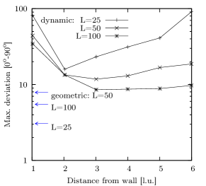
Figure 4: The maximum error of a normal vector (measured as the angle between numerical and exact vectors) for two numerical methods in a three-dimensional ball. Arrows represent geometric normals computed with Eq. (4) using $\gamma=1$ and $r=4$.

Fig. 4 depicts the maximum error between geomeric and exact normals. Results are compared to dynamic normals at various distances from the wall [45]. Geometric normals are found to be more accurate.

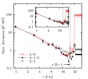
Figure 5: (color online) The maximum error of geometric normal (4) for three values of $\gamma$ as a function of the averaging radius $r$ in a three-dimensionall ball and tube (inset) with radii $R$=25.

To test the influence of the averaging radius on the accuracy of the normal for various exponents $\gamma$ we vary $r$ and calculate the error on a ball and a tube of radii $R$. The resulting error is a non-monotonous function of $r$ with a minimum at at $r/R=1$ (see Fig. 5). At $r/R>1$ the mean error for $\gamma=0$ grows rapidly whereas for $\gamma\neq 0$ it remains constant (with slight favour to $\gamma=1/2$). A large error for $r/R>1$ for $\gamma=0$ comes from the fact that the averaging area covers the entire object, the resulting normal is $0$, and the information on the object geometry vanishes. If $\gamma\neq 0$, the problem is avoided because normal vectors defined on facets on the boundary lying on the opposite side of the object have much lower weights.

4 Wall shear stress in a channel flow

In this section we test the accuracy of the WSS equation (2) combined with geometric normals in an inclined and bent channel flows.

4.1 Inclined channel

A two-dimensional channel of an initial resolution $120\times 20$ lattice units (l.u.) was inclined at angle $\alpha$ to the $x$ axis so that the radii of the inlet and outlet were kept constant. The analytical velocity profile (Poiseuille flow) was imposed on the inlet and outlet boundaries. The lattice viscosity was $\nu=0.01$ and the maximum velocity in the channel center was $u_{max}=0.01$ (lattice units). Using deviations from the analytical velocity field we found the steady state in less than $10^{4}$ iterations. We ran the flow for $\tan\alpha\in[0;2]$ and calculated dynamical and geometrical normal vectors in a strip of length $80$ l.u. (centered horizontally).

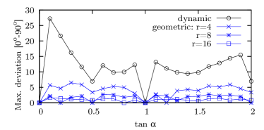
Figure 6: (color online) The maximum error of geometrical and dynamical normal in a channel at various inclination angles. For geometrical scheme three $r$ are tested.

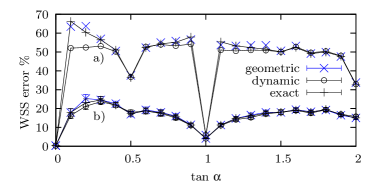
Figure 7: (color online) The maximum (a) and average (b) over $80$ neighbouring sites of the error of WSS computed using various types of normal vectors in a channel at various inclination angles. Error bars in the average represent the standard error.

In Fig. 6 the maximum angle between the numerical and exact vectors is given as a function of the channel inclination angle. The error of the geometric procedure decreases with $r$ and is smaller than for the dynamic scheme. The most accurate results were obtained for $\tan\alpha=0$ and $\tan\alpha=1$.

Next, we compute WSS using Eq. (2) and show that in an inclined channel WSS is essentially independent of the choice of the normal vector type (Fig. 7). This implies that the largest contribution to the error comes from the velocity field near the staircase boundary. This fact is also visible in Fig. 6 where the large error of dynamic normals is caused by the velocity field inaccuracy. The maximum relative error of numerical WSS calculated at a single node is much larger than the error of the mean taken over 80 nodes. Therefore one could use an equation similar to Eq. 4, where a spatial average of WSS in a vicinity of the wall element is computed:

$$\boldsymbol{\tau}=\left(\sum_{i}w_{i}\right)^{-1}\sum_{i}w_{i}\boldsymbol{\tau}_{i},$$ (5)

where $w_{i}$ are weights of the same form as used for normals. However, we leave applicability of Eq. (5) to more complex flows as an open problem.

4.2 Bent channel

Next, we investigate the flow in a two-dimensional bent channel geometry defined by its inner and outer radii ($R_{1}$ and $R_{2}$, respectively). For the mesh of resolution $W\times H$ a site placed at $(i,j)$ is of fluid type if $R_{1}<|(i-W/2,j)|<R_{2}$, otherwise it is a no-slip site (or it is excluded). We take $R_{1}=10$ and $R_{2}=20$ and the mesh resolution $45\times 25$ l.u. and run the steady state simulation with $\nu=0.01$ and analytical inlet/outlet boundary conditions.

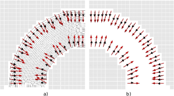
Figure 8: (color online) Exact normals in a bent channel flow (short arrows) compared to dynamic (a) and geometric (b) normals. Boundary cells are empty and only part of the channel is shown for both methods (the other parts are symmetric).

We calculated normals using both procedures and compare them visually against exact normals (Fig. 8). To understand the influence of the flow field near staircase wall on dynamic normals the flow field is shown using streamlines (Fig. 8 a). We determined the angle between each individual pair of numerical and exact vectors using the data from Fig. 8 and found the maximum error of the dynamic scheme to be around 25^∘. For the geometric scheme the error is kept below 10^∘. The average errors are calculated as $10.8^{\circ}$ and $3.9^{\circ}$ for dynamic and geometric vectors, respectively.

Figure 9: WSS components in the bent channel flow computed with Eq. (2) at various angular positions ($2$ l.u. from the inner channel wall). Results are obtained using geometric (squares) and dynamic (circles) normals. Empty and filled symbols represent the $x$ and $y$ component, respectively. Data are normalized by $\tau_{\mathrm{ref}}=\max(\tau_{i})$.

Then we computed WSS at the inner wall at various angular positions and plotted its components against exact solutions (Fig. 9). The numerical data follow the analytical solutions. Regions of larger deviations may be recognized (e.g. $\tau_{y}$ at $\alpha\in(20,40)$) mostly because WSS was calulated at the first node next to the boundary. An interesting observation may be done for the central region ($\alpha\in(80,100)$) where introduction of the geometric normals slightly decreased the error for $\tau_{x}$ (similarly for $\tau_{y}$). The reason could be that the central part of the bent channel is horizontally flat in the grid representation (see Fig. 8) and the velocity field follows the geometry. Therefore, the resulting dynamic normals are almost perpendicular to the surface whereas they are not in the original geometry (a bent inner circle). This results in a large systematic deviation of the $x$ component of WSS which is slightly decreased if more accurate geometric normals are used.

5 A flow through the human abdominal aorta

Finally, we test the procedures described in previous sections in a real situation and compute WSS in an abdominal aorta model based on patient-specific data. For this purpose we utilize data from the Virtual Family (VF) [51] – a freely available library of high resolution anatomical human body models based on MRI measurements. We use Eq. (2) to compute the geometric normals and Eq. (3) for WSS.

5.1 Data preparation

From several models provided by the VF we chose Duke – a 34 year old man. Using the software included in VF we manually selected a part of his abdominal aorta 17.8 cm over and 5.2 cm under the bifurcation point. We exported voxel data as .raw files that encode a tissue type with integers. Then we used the CVMLCPP library [52] ray marching algorithm to approximate the artery surface. The resulting mesh was of very poor quality, therefore further smoothing was done using MeshLab [53]. At this point we either voxelized the mesh to get various grid resolutions for the LBM or continued meshing until we obtained a three-dimensional unstructured volumetric mesh using NETGEN [54]. Next we applied the boundary conditions and exported the mesh in the neutral NETGEN format for further use in FVM software.

5.2 Simulation

First, we ran the steady state LBM simulation using the Sailfish library adjusted for our purposes. We imposed a flat velocity profile on the inlet and zero pressure at both outlets of the model. Due to the tortuous geometry of the aorta the flat inlet velocity causes a macroscopic flow with a slightly lower effective flowrate. We used the following parameters: $u_{0,p}=0.0764$ m/s (the velocity at inlet), $l_{0,p}=0.03$ m (the diameter of the inlet), $\nu=3\cdot 10^{-6}$ m²/s (kinematic viscosity of the fluid), $\varrho_{p}=1000$ kg/m³ (the fluid density). Thus, the characteristic time $t_{0,p}=l_{0,p}/u_{0,p}=0.393$ s and the Reynolds number Re=300 (based on an effective flowrate). The model was subdivided into $461\times 108\times 163$ voxels ($5$mm resolution). The number of grid nodes along the inlet diameter was $N$=60, thus $\delta x=0.0166$. We chosed $u_{lb}=0.125$, for which $\delta t=u_{lb}\cdot\delta x=0.00208$ was found. The final lattice viscosity $\nu_{lb}=\delta t/\delta x^{2}\cdot 1/\mathrm{Re}=0.0098$ was found. We continued the simulation until the steady stade was reached (41 000 time steps) based on the observation of the velocity and pressure field convergence. The resulting distribution function that describes the steady state was used in Eq. (2) to get WSS at $2$ l.u. away from the boundary. We used our geometric normals in Eq. (2) as well as to move away from the boundary nodes. We first computed a dimensionless counterpart of $\tau_{lb}$, namely $\tau_{d}=\varrho_{lb}\cdot\delta x^{2}/\delta t^{2}\cdot\tau_{lb}=63.7\tau_{lb}$. Then, the stress in [Pa] was obtained using $\tau_{p}=\varrho_{p}\cdot l_{0,p}/t_{0,p}\cdot\tau_{d}=5.84\tau_{d}$.

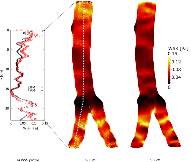
Figure 10: (color online) Wall shear stress calculated using LBM and FVM. The lighter the color, the larger WSS acts on the surface.

Second, we ran the same steady flow using finite volume Semi Implicit Method for Pressure Linked Equations (SIMPLE) [55]. We used simpleFoam solver from OpenFOAM [56] with previously generated mesh built of 496 656 tetrahedral elements. We applied a constant flowrate condition at the inlet with the flowrate Q=$2.1206\cdot 10^{-5}$ [m³/s] corresponding to $Re=300$. The zero pressure and zero velocity gradient was applied at both outlets. We stopped the simulation after 1 second and confirmed that the convergence criteria was met (the initial and final residuals of pressure and velocity was smaller than $10^{-5}$). Then, we computed WSS using standard OpenFOAM tools.

The resulting WSS in the abdominal aorta model computed with both methods is visualized as a color map (Fig. 1 and Fig. 10). The resulting ranges of WSS were $(6.74\cdot 10^{-5},0.32)$ for LBM and $(0,0.42)$ for FVM. We found that the discrepancy in maximum values is due to the extreme values at the very boundary conditions, thus we encoded the WSS magnitude in the range of WSS $\in(0,0.15)$ [Pa] only for better visualization. The profile of WSS (Fig. 10 a) is taken along the white dashed line (see Fig. 10 b) from a gray scale projection of the results onto a plane.

The peak value in the bifurcation area is around $0.12$ [Pa] as observed in two branches behind the bifurcation point where the wavy profile of WSS may be easily recognized. The wavy profile of WSS seems to be mainly an effect of the geometry: the smaller profile diameter, the larger WSS. The quantitative comparison of WSS between LBM and WSS (Fig. 10 a) shows an excellent agreement in the area not influenced by boundary conditions.

Next, we compare the WSS magnitudes obtained for both methods with the experimental data measured using the laser photochromic dye tracer technique [57]. There, for similar conditions (the abdominal aorta of the healthy 35-year-old subject at rest and the steady flow) and the Reynolds number $Re=227$ (based on the inlet flowrate) the measurement values of WSS were in the range $\tau\in(0.06,0.3)$ [Pa]. We found our numerical computations agree well with the experimental data. The remaining difference in the minimum value of WSS is most probably an effect of the patient-specific geometry as we found the minimum of WSS in Fig. 10a at $y=16$cm, where the enlargement of the cross-section of our aorta model is clearly noticeable.

6 Discussion

Comparison of normal vectors computed for three-dimensional objects with two different methods given in Sec. 3.1 indicates an improvement in accuracy of our procedure against the dynamic scheme based on the velocity field. The improvement is significant e.g. close to the wall for a small lattice the error for dynamic normals is close to $90^{\circ}$ but it remains below $10^{\circ}$ in our method (Fig.6). Additional tests in the flow through an inclined (Fig. 6) and bent (Fig. 8) channel flows confirm higher accuracy of geometric normals. Application of the geometric normals gives practically the same WSS as when its dynamic or exact counterparts are used in an inclined channel. In the bent channel, however, some differences are visible if separate stress components are analyzed (see Fig. 9). We found a region of an increased WSS accuracy based on the geometric normals (central part of the inner wall). We believe this observations favorize the use of our scheme as it is simpler, more efficient (fewer algebraic operations) and provides the sense of the normal. We are aware that our method is nonlocal which may lead to complications in parallel implementation, this, however, might be solved e.g. by using algorithms that utilize fast shared memory of GPU processors.

Our tests in a real patient-based geometry show an excellent agreement with a standard finite volume solver. The WSS in the fluid flow through the abdominal aorta is both qualitatively and quantitatively the same in LBM and FVM (see Fig. 10). The slight difference between both methods at inlets and outlets is an effect of differences in the boundary conditions used. The data in Fig. 10 a) give an impression of what is a typical length scale at which the imposed inlet boundary conditions play a role in hemodynamical simulations (e.g. we got around $10$ cm from the inlet for the given setup).

To get acceptable matching of the results in Fig. 10 we moved the computation 2 nodes away from the wall (as suggested in [45]). This procedure has, however, some limitations. First, while producing color-maps of WSS we noticed some missing nodes (see discontinuity in Fig. 10b just above the bifurcation point). The reason for it is the following: if we start from two neighbouring sites and move some distance along their normals, the destination nodes no longer have to be neighbours (especially if normals were pointing in different directions) and empty nodes at the surface may be visible. This artifact does not influence WSS values obtained. To produce decent visualization one could additionaly compute WSS for those empty sites, e.g. in the Fig. 1 we visualize WSS at a distances d=2 and at d=0 which practically eliminated the problem of empty sites. Second, moving away from boundary may be unwanted in general because one could argue the quantity is no longer the wall shear stress but rather a near-the-wall shear stress. To make the use of the information at the wall surface only, we suggested averaging of WSS at the wall in the neighbourhood of a site for which WSS is calculated (see Eq. 5). Averaging decreased the error of WSS at almost each site of the inclined channel flow by more than 50% (see Fig. 7). To make the WSS averaging procedure a part of a complete protocol one should further test its behavior for smaller averaging radii and various three-dimensional geometries.

We found that for a single model the preparation of FVM mesh described in Sec. 5.1 takes around an hour without data segmentation (the Virtual Family implements this). In contrast, LBM could utilize the segmented MRI/CT data directly and skip the meshing process. We can imagine that, if the gray level was decoded correctly into some of physical variables used in LBM simulation (e.g. endothelial wall roughness) then these data could be used directly without segmentation. In this way one could turn the largest weakness of the LBM method (staircase approximation of the boundary) into its strongest point in hemodynamical applications (no need for tedious data preprocessing), where our simple procedure for normals would be of high importance.

7 Conclusions

There are several reasons why one would want to calculate the wall orientation in LBM using the geometric procedure described here. First, our method gives a gain in accuracy over dynamic normals. Second, the computation overhead is much smaller as the averaging is done using a few simple algebraic operations rather than by solving an eigenvalue problem. Third, we showed that our procedure gives practically the same WSS as if exact normals were used. Fourth, the computation of geometric normals is – by definition – independent of the Reynolds number whereas dynamic normals are dependent on Re, which is unphysical. Fifth, it is suitable for the time dependent flows. Sixth, the given scheme provides the sense of normals that might be crucial in the calculations that require determination of separated wall shear stress components e.g. oscillating shear index and wall shear stress gradient.

8 Acknowledgement

The publication has been prepared as part of the project of the City of Wrocław, entitled – “Green Transfer” – academia-to-business knowledge transfer project co-financed by the European Union under the European Social Fund, under the Operational Programme Human Capital (OP HC): sub-measure 8.2.1 (MM). ZK was supported by MNiSW grant No. N 519 437939. We acknowledge support and discussions from Dominik Szczerba, Jakub Kominiarczuk, Ziemowit Malecha, Michał Januszewski, Jonas Latt and Bastien Chopard. Additionaly to the software mentioned in the text we used also Palabos, Paraview and Techdig. We gratefully acknowledge hardware donation from Nvidia.

Appendix A The stress on arbitrary plane in LBM

The stress tensor in fluids is a sum of pressure and viscous terms:

$$\sigma_{ij}=-p\delta_{ij}+\sigma_{ij}^{\prime}.$$ (6)

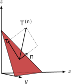
Figure 11: (color online) The overall stress $\mathbf{T}^{(n)}$ and its tangential part $\boldsymbol{\tau}$.

The Cauchy formula gives the overall stress on the wall with a normal vector $\mathbf{n}$ (Fig. 11):

$$T^{(\mathbf{n})}_{i}=\sigma_{ij}n_{j}.$$ (7)

The shear stress may be computed as the difference between the overall stress and its projection onto the normal:

$$\tau_{i}=\sigma_{ij}n_{j}-(\sigma_{kj}n_{j}n_{k})n_{i}.$$ (8)

We insert Eq. (6) into Eq. (8), and since $\delta_{jk}n_{j}n_{k}=1$, the equation for WSS reads:

$$\tau_{i}=\sigma^{\prime}_{ij}n_{j}-(\sigma^{\prime}_{kj}n_{j}n_{k})n_{i}.$$ (9)

For the incompressible, Newtonian fluid the viscous stress $\sigma^{\prime}_{ij}$ is a linear function of the rate of strain $\varepsilon_{ij}$:

$$\sigma_{ij}^{\prime}=2\mu\varepsilon_{ij}.$$ (10)

Combination of Eq. (9) and Eq. (10) gives:

$$\tau_{i}=2\mu\left(\varepsilon_{ij}n_{j}-\left(\varepsilon_{kj}n_{j}n_{k}\right)n_{i}\right).$$ (11)

A definition of the rate of strain tensor in LBM, which uses the non-equilibrium part of the distribution function reads:

$$\varepsilon_{ij}=\frac{\omega}{2c_{s}^{2}\varrho}\sum_{\alpha}f_{\alpha}^{neq}c_{\alpha i}c_{\alpha j},$$ (12)

where $f_{\alpha}^{neq}=f_{\alpha}-f_{\alpha}^{eq}$ and $f_{\alpha}^{eq}$ is an equilibrium Maxwell-Boltzmann distribution. Finally, we combine Eqs. (11) and (12) and and get Eq. (2).

Appendix B WSS algorithm

  $dim\leftarrow 3$

  $C\leftarrow(\mu\omega)/(c_{s}^{2}\varrho)$

  for $i=0\to dim-1$ do

     $sum\alpha\leftarrow 0$

     for all $\alpha$ do

        $sumk\leftarrow 0$

        for $k=0\to dim-1$ do

           $sumk\leftarrow sumk+c_{\alpha k}n_{i}n_{k}$

        end for

        $sumj\leftarrow 0$

        for $j=0\to dim-1$ do

           $sumj\leftarrow sumj+c_{\alpha j}n_{j}\left(c_{\alpha i}-sumk\right)$

        end for

        $f_{\alpha}^{neq}\leftarrow f_{\alpha}-f_{\alpha}^{eq}$

        $sum\alpha\leftarrow sum\alpha+f_{\alpha}^{neq}\cdot sumj$

     end for

     $\tau_{i}\leftarrow C\cdot sum\alpha$

  end for

  $WSS\leftarrow|\boldsymbol{\tau}|$

Algorithm 1 Calculation of WSS from Eq. (2).

References

- Ku [1997] D. N. Ku, Blood Flow In Arteries, Annual Review of Fluid Mechanics 29 (1) (1997) 399–434.
- Berger and Jou [2000] S. A. Berger, L.-D. Jou, Flows in Stenotic Vessels, Annual Review of Fluid Mechanics 32 (1) (2000) 347–382.
- Anor et al. [2010] T. Anor, L. Grinberg, H. Baek, J. R. Madsen, M. V. Jayaraman, G. E. Karniadakis, Modeling of blood flow in arterial trees, Wiley Interdisciplinary Reviews: Systems Biology and Medicine 2 (5) (2010) 612–623.
- Dai et al. [2004] G. Dai, M. R. Kaazempur-Mofrad, S. Natarajan, Y. Zhang, S. Vaughn, B. R. Blackman, R. D. Kamm, G. García-Cardeña, M. A. Gimbrone, Distinct endothelial phenotypes evoked by arterial waveforms derived from atherosclerosis-susceptible and -resistant regions of human vasculature, Proceedings of the National Academy of Sciences of the United States of America 101 (41) (2004) 14871–14876.
- Cebral et al. [2004] J. R. Cebral, M. A. Castro, J. E. Burgess, R. S. Pergolizzi, M. J. Sheridan, C. M. Putman, Characterization of cerebral aneurysm for assessing risk of rupture using patient-specific computational hemodynamics models, AJNR American Journal of Neuroradiology 2005 (2004) 2550–2559.
- Nesbitt et al. [2009] W. S. Nesbitt, E. Westein, F. J. Tovar-Lopez, E. Tolouei, A. Mitchell, J. Fu, J. Carberry, A. Fouras, S. P. Jackson, A shear gradient-dependent platelet aggregation mechanism drives thrombus formation., Nature Medicine 15 (6) (2009) 665–673.
- Papaioannou and Stefanadis [2005] T. G. Papaioannou, C. Stefanadis, Vascular wall shear stress: basic principles and methods, Hellenic journal of cardiology HJC Hellenike kardiologike epitheorese 46 (1) (2005) 9–15.
- Ku et al. [1985] D. Ku, D. Giddens, C. Zarins, S. Glagov, Pulsatile flow and atherosclerosis in the human carotid bifurcation. Positive correlation between plaque location and low oscillating shear stress, Arteriosclerosis, Thrombosis, and Vascular Biology 5 (3) (1985) 293–302.
- Shaaban and Duerinckx [2000] A. M. Shaaban, A. J. Duerinckx, Wall Shear Stress and Early Atherosclerosis, American Journal of Roentgenology 174 (6) (2000) 1657–1665.
- Cecchi et al. [2011] E. Cecchi, C. Giglioli, S. Valente, C. Lazzeri, G. F. Gensini, R. Abbate, L. Mannini, Role of hemodynamic shear stress in cardiovascular disease, Atherosclerosis 214 (2) (2011) 249 – 256.
- Boussel et al. [2008] L. Boussel, V. Rayz, C. McCulloch, A. Martin, G. Acevedo-Bolton, M. Lawton, R. Higashida, W. S. Smith, W. L. Young, D. Saloner, Aneurysm Growth Occurs at Region of Low Wall Shear Stress, Stroke 39 (11) (2008) 2997–3002.
- Tse et al. [2011] K. M. Tse, P. Chiu, H. P. Lee, P. Ho, Investigation of hemodynamics in the development of dissecting aneurysm within patient-specific dissecting aneurismal aortas using computational fluid dynamics (CFD) simulations, Journal of Biomechanics 44 (5) (2011) 827 – 836.
- Reneman et al. [2006] R. S. Reneman, T. Arts, A. P. G. Hoeks, Wall shear stress–an important determinant of endothelial cell function and structure–in the arterial system in vivo. Discrepancies with theory., Journal of Vascular Research 43 (3) (2006) 251–269.
- Caro [2009] C. Caro, Discovery of the Role of Wall Shear in Atherosclerosis, Arterioscler. Thromb. Vasc. Biol. 29 (2009) 158–161.
- Jou et al. [2008] L.-D. Jou, D. Lee, H. Morsi, M. Mawad, Wall Shear Stress on Ruptured and Unruptured Intracranial Aneurysms at the Internal Carotid Artery, American Journal of Neuroradiology 29 (9) (October 2008) 1761–1767.
- Carallo et al. [2006] C. Carallo, L. F. Lucca, M. Ciamei, S. Tucci, M. S. de Franceschi, Wall shear stress is lower in the carotid artery responsible for a unilateral ischemic stroke, Atherosclerosis 185 (1) (2006) 108 – 113.
- Meyerson et al. [2001] S. L. Meyerson, C. L. Skelly, M. A. Curi, U. M. Shakur, J. E. Vosicky, S. Glagov, L. B. Schwartz, The effects of extremely low shear stress on cellular proliferation and neointimal thickening in the failing bypass graft, Journal of Vascular Surgery 34 (1) (2001) 90 – 97.
- Malek et al. [1999] A. M. Malek, S. L. Alper, S. Izumo, Hemodynamic shear stress and its role in atherosclerosis, Jama The Journal Of The American Medical Association 282 (21) (1999) 2035–42.
- Paszkowiak and Dardik [2003] J. J. Paszkowiak, A. Dardik, Arterial Wall Shear Stress: Observations from the Bench to the Bedside, Vascular and Endovascular Surgery 37 (1) (January/February 2003) 47–57.
- Pantos et al. [2007] J. Pantos, E. Efstathopoulos, D. G. Katritsis, Vascular Wall Shear Stress in Clinical Practice, Current Vascular Pharmacology 5 (2) (2007) 113–119.
- Milner et al. [1998] J. S. Milner, J. A. Moore, B. K. Rutt, D. A. Steinman, Hemodynamics of human carotid artery bifurcations: computational studies with models reconstructed from magnetic resonance imaging of normal subjects., J Vasc Surg 28 (1) (1998) 143–56.
- Quarteroni et al. [2000] A. Quarteroni, M. Tuveri, A. Veneziani, Computational vascular fluid dynamics: problems, models and methods, Computing and Visualization in Science 2 (2000) 163–197, ISSN 1432-9360, 10.1007/s007910050039.
- Gohil et al. [2011] T. Gohil, R. McGregor, D. Szczerba, K. Burckhardt, K. Muralidhar, G. Székely, Simulation of Oscillatory Flow in an Aortic Bifurcation Using FVM and FEM: a Comparative Study of Implementation Strategies, International Journal for Numerical Methods in Fluids 66 (8) (2011) 1037–1067.
- Nickolls and Dally [2010] J. Nickolls, W. J. Dally, The GPU Computing Era, IEEE Micro 30 (2010) 56–69.
- Aidun and Clausen [2011] C. K. Aidun, J. R. Clausen, Lattice-Boltzmann Method for Complex Flows, Annual Review of Fluid Mechanics 42 (1) (2011) Annual Reviews—472.
- Pohl et al. [2004] T. Pohl, F. Deserno, N. Thurey, U. Rude, P. Lammers, G. Wellein, T. Zeiser, Performance Evaluation of Parallel Large-Scale Lattice Boltzmann Applications on Three Supercomputing Architectures, in: Proceedings of the 2004 ACM/IEEE conference on Supercomputing, SC ’04, IEEE Computer Society, Washington, DC, USA, 21–, 2004.
- Peters et al. [2010] A. Peters, S. Melchionna, E. Kaxiras, J. Lätt, J. Sircar, M. Bernaschi, M. Bison, S. Succi, Multiscale Simulation of Cardiovascular flows on the IBM Bluegene/P: Full Heart-Circulation System at Red-Blood Cell Resolution, in: Proceedings of the 2010 ACM/IEEE International Conference for High Performance Computing, Networking, Storage and Analysis, SC ’10, IEEE Computer Society, Washington, DC, USA, 1–10, 2010.
- Harvey et al. [2008] M. J. Harvey, G. De Fabritiis, G. Giupponi, Accuracy of the lattice-Boltzmann method using the Cell processor, Phys. Rev. E 78 (2008) 056702.
- Peng et al. [2008] L. Peng, K.-I. Nomura, T. Oyakawa, R. K. Kalia, A. Nakano, P. Vashishta, Parallel Lattice Boltzmann Flow Simulation on Emerging Multi-core Platforms, in: Proceedings of the 14th international Euro-Par conference on Parallel Processing, Euro-Par ’08, Springer-Verlag, Berlin, Heidelberg, ISBN 978-3-540-85450-0, 763–777, 2008.
- Tölke and Krafczyk [2008] J. Tölke, M. Krafczyk, TeraFLOP computing on a desktop PC with GPUs for 3D CFD, Int. J. Comput. Fluid Dyn. 22 (7) (2008) 443–456.
- Xian and Takayuki [2011] W. Xian, A. Takayuki, Multi-GPU performance of incompressible flow computation by lattice Boltzmann method on GPU cluster, Parallel Computing 37 (February) (2011) 521–535.
- He and Luo [1997] X. He, L.-S. Luo, Lattice Boltzmann Model for the Incompressible Navier–Stokes Equation, Journal of Statistical Physics 88 (1997) 927–944.
- Cosgrove et al. [2003] J. A. Cosgrove, J. M. Buick, S. J. Tonge, C. G. Munro, C. A. Greated, D. M. Campbell, Application of the lattice Boltzmann method to transition in oscillatory channel flow, Journal of Physics A: Mathematical and General 36 (10) (2003) 2609.
- Artoli et al. [2006] A. Artoli, A. Hoekstra, P. Sloot, Mesoscopic simulations of systolic flow in the human abdominal aorta, Journal of Biomechanics 39 (5) (2006) 873+.
- Axner et al. [2009] L. Axner, A. G. Hoekstra, A. Jeays, P. Lawford, R. Hose, P. M. Sloot, Simulations of time harmonic blood flow in the Mesenteric artery: comparing finite element and lattice Boltzmann methods, BioMedical Engineering Online 8 (2009) 23.
- Bernsdorf and Wang [2009] J. Bernsdorf, D. Wang, Non-Newtonian blood flow simulation in cerebral aneurysms, Comput. Math. Appl. 58 (2009) 1024–1029.
- Palabos [2012] Palabos, http://www.palabos.org/, 2012.
- Chopard et al. [2010a] B. Chopard, D. Lagrava, O. Malaspinas, R. Ouared, J. Latt, K.-O. Lovblad, V. Pereira-Mendes, A Lattice Boltzmann Modeling of Bloodflow in Cerebral Aneurysm, in: V European Conference on Computational Fluid Dynamics, ECCOMAS CFD, 2010a.
- Chopard et al. [2010b] B. Chopard, R. Ouared, A. Deutsch, H. Hatzikirou, D. Wolf-Gladrow, Lattice-Gas Cellular Automaton Models for Biology: From Fluids to Cells, Acta Biotheoretica 58 (2010b) 329–340.
- He et al. [2009] X. He, G. Duckwiler, D. J. Valentino, Lattice Boltzmann simulation of cerebral artery hemodynamics, Computers & Fluids 38 (4) (2009) 789 – 796.
- Krüger et al. [2009] T. Krüger, F. Varnik, D. Raabe, Shear stress in lattice Boltzmann simulations, Phys. Rev. E 79 (2009) 046704.
- Krüger et al. [2010] T. Krüger, F. Varnik, D. Raabe, Second-order convergence of the deviatoric stress tensor in the standard Bhatnagar-Gross-Krook lattice Boltzmann method, Phys. Rev. E 82 (2010) 025701.
- Boyd et al. [2005] J. Boyd, J. Buick, J. A. Cosgrove, P. Stansell, Application of the lattice Boltzmann model to simulated stenosis growth in a two-dimensional carotid artery, Physics in Medicine and Biology 50 (20) (2005) 4783.
- Pontrelli et al. [2011] G. Pontrelli, C. S. König, I. Halliday, T. J. Spencer, M. W. Collins, Q. Long, S. Succi, Modelling wall shear stress in small arteries using the Lattice Boltzmann method: influence of the endothelial wall profile 33 (7) (2011) 832 – 839, micro and Nano Flows 2009 - Biomedical Stream - 2nd Micro and Nano Flows Conference.
- Stahl et al. [2010] B. Stahl, B. Chopard, J. Latt, Measurements of wall shear stress with the lattice Boltzmann method and staircase approximation of boundaries, Computers & Fluids 39 (9) (2010) 1625–1633.
- McNamara and Zanetti [1988] G. R. McNamara, G. Zanetti, Use of the Boltzmann Equation to Simulate Lattice-Gas Automata, Phys. Rev. Lett. 61 (1988) 2332–2335.
- Higuera and Jiménez [1989] F. J. Higuera, J. Jiménez, Boltzmann Approach to Lattice Gas Simulations, EPL (Europhysics Letters) 9 (7) (1989) 663.
- d’Humieres et al. [2002] D. d’Humieres, I. Ginzburg, M. Krafczyk, P. Lallemand, L. S. Luo, Multiple-Relaxation-Time Lattice Boltzmann Models in Three Dimensions, Philosophical Transactions: Mathematical, Physical and Engineering Sciences 360 (1792) (2002) 437+.
- Luo [2000] L.-S. Luo, Theory of the lattice Boltzmann method: Lattice Boltzmann models for nonideal gases, Phys. Rev. E 62 (2000) 4982–4996.
- Sailfish [2012] Sailfish, http://sailfish.us.edu.pl/, 2012.
- Christ et al. [2010] A. Christ, W. Kainz, E. G. Hahn, K. Honegger, M. Zefferer, E. Neufeld, W. Rascher, R. Janka, W. Bautz, J. Chen, B. Kiefer, P. Schmitt, H.-P. Hollenbach, J. Shen, M. Oberle, D. Szczerba, A. Kam, J. W. Guag, N. Kuster, The Virtual Family development of surface-based anatomical models of two adults and two children for dosimetric simulations, Physics in Medicine and Biology 55 (2) (2010) N23.
- CVMLCPP [2012] CVMLCPP, http://tech.unige.ch/cvmlcpp/, 2012.
- MeshLab [2012] MeshLab, meshlab.sourceforge.net/, 2012.
- NETGEN [2012] NETGEN, http://www.hpfem.jku.at/netgen/, 2012.
- Patankar [1980] S. V. Patankar, Numerical heat transfer and fluid flow, Hemisphere Pub. Corp. ; McGraw-Hill, Washington : New York :, 1980.
- OpenFoam [2012] OpenFoam, http://www.openfoam.com/, 2012.
- Bonert et al. [2003] M. Bonert, R. L. Leask, J. Butany, C. R. Ethier, J. G. Myers, K. W. Johnston, M. Ojha, The relationship between wall shear stress distributions and intimal thickening in the human abdominal aorta., Biomed Eng Online 2 (2003) 18.