Nearly extensive sequential memory lifetime achieved by coupled nonlinear neurons

Abstract

Many cognitive processes rely on the ability of the brain to hold sequences of events in short-term memory. Recent studies have revealed that such memory can be read out from the transient dynamics of a network of neurons. However, the memory performance of such a network in buffering past information has only been rigorously estimated in networks of linear neurons. When signal gain is kept low, so that neurons operate primarily in the linear part of their response nonlinearity, the memory lifetime is bounded by the square root of the network size. In this work, I demonstrate that it is possible to achieve a memory lifetime almost proportional to the network size, “an extensive memory lifetime”, when the nonlinearity of neurons is appropriately utilized. The analysis of neural activity revealed that nonlinear dynamics prevented the accumulation of noise by partially removing noise in each time step. With this error-correcting mechanism, I demonstrate that a memory lifetime of order $N/\log N$ can be achieved.

Keywords:

working memory, memory lifetime, nonlinear dynamics, error-correcting

1 Introduction

Buffering a sequence of events in the activity of neurons is an important property of the brain that is necessary to carry out many cognitive tasks Baddeley, (2000); Münte et al., (1998); de Fockert et al., (2001); Orlov et al., (2000); Pastalkova et al., (2008); Hahnloser et al., (2002); Baeg et al., (2003). The fundamental limit of the capacity of the sequential memory is, however, largely unknown. Several works have suggested that a long memory lifetime can arise as a network property of neurons, where individual neurons typically have limited memory Goldman, (2009); White et al., (2004); Lim and Goldman, (2011). However, the structures and operating regimes suitable for a network of neurons to buffer a sequence of events is also unknown. This paper investigates the limit of such sequential memory for buffering past stimuli in the presence of dynamical noise. More specifically, we examine how reconstructions of past stimuli degrade as we trace them back into the past. This kind of working memory generally improves with the size of the network. Hence, important questions are: How the memory lifetime scales with network size, and what kind of network structure achieves the longest memory lifetime. The scaling of the memory lifetime to the network size has been rigorously characterized only under limited conditions White et al., (2004); Ganguli et al., (2008). In particular, the memory lifetime for non-saturating linear neurons can be proportional to the network size, $N$, which is, from an information theoretical perspective, the best possible situation for reconstructing all sequences of non-sparse input Ganguli and Sompolinsky, (2010). This is called the extensive memory lifetime. Ganguli et al. also estimated the memory lifetime of a network of neurons with response nonlinearity but under a rather restricted condition where the signal gain was kept small so that neurons operated in their linear regime. Under this condition, the sequential memory lifetime is upper-bounded by $\sim\sqrt{N}$ Ganguli et al., (2008). However, as we will see in the following, fine-tuning of a network parameter is necessary for this to work.

I explore in this paper a network structure that yields a long-lasting sequential memory that is longer than the bound previously set for nonlinear neurons. The network structure that I explore is a simple feedforward network with a fixed number of neurons in one layer. This network architecture has been studied in the context of synchronous-firing chains, i.e., synfire chains Abeles, (1982); Bienenstock, (1995); Herrmann et al., (1995); Diesmann et al., (1999); Rossum et al., (2002); Vogels and Abbott, (2005); Kumar et al., (2008). In the current context, reliable propagation of synfire activity is used to maintain information on past sequences. Although reliable propagation of synfire activity in the presence of noise has been reported several times, quantitative characterization of such reliability has been only partially achieved. In particular, previous studies did not systematically evaluate the effect of occasional strong noise that spontaneously ignites or blocks synfire activity Herrmann et al., (1995); Bienenstock, (1995). As we will see, this occasional large noise prevents a network from achieving an extensive memory lifetime. The scaling of the memory lifetime to the network size in the presence of such noise has not yet been reported to my knowledge.

In this paper, I analytically evaluate the effects of response nonlinearity and noise on the performance of sequential memory. The main result is the following: If we require a network of $N$ neurons to hold $I$ bits of information about stimulus presented at each time, the achievable memory lifetime is proportional to $(N/I)/\log(N/I)$, which is much longer than the previously proposed order $\sqrt{N}$ memory, assuming a small gain. Moreover, the nonlinear dynamics of neurons drastically improves the tolerance of working-memory to noise levels, compared to the previously proposed semi-linear dynamical regime. Numerical simulations show that complex firing sequences of leaky integrate-and-fire neurons are successfully buffered by this network architecture.

2 Result

In order to derive the memory lifetime of feedforward networks, I consider a simple firing-rate model of neurons with saturating response nonlinearity. We first aim at reconstructing a sequence of binary input but we will show later that it is straightforward to generalize this scheme to reconstruct sequences of analog input.

2.1 Evaluating the memory lifetime for interacting nonlinear neurons

To study what effects response nonlinearity has on the memory lifetime in a simple system, we consider the dynamics of a homogeneous feedforward network of $L$ layers (see, Fig.1), where each layer has $n$ neurons, and the total number of neurons in the network is given by $N=nL$. Let us consider discrete-time dynamics here for the sake of simplicity. The activity of neuron $i$ in layer $l+1$ at time $t+1$ is modeled as

$$r_{i}(t+1)=\phi\left(\sum_{j\in\mathcal{S}_{l}}w_{ij}r_{j}(t)+\sigma\xi_{i}(t+1)\right),$$ (1)

where $\phi$ is the response nonlinearity, $\mathcal{S}_{l}$ is a set of $n$ neurons in layer $l$, $w_{ij}=1/n$ is the uniform synaptic strength from neuron $j$ in layer $l$ to neuron $i$ in layer $l+1$, $\sigma$ is the magnitude of noise, and $\xi_{i}$ is an independent white Gaussian random variable of unit variance that describes the postsynaptic noise to neuron $i$. Here, in order to better distinguish the effect of the nonlinearity from the signal-to-noise ratio, we fix the magnitude of synaptic strength and instead change the slope of the nonlinearity and the parameter $\sigma$ that controls the noise level relative to the input from the previous layer. The time-dependent input to the network is described by $r_{0}(t)$ and fed only to the first layer. For simplicity, we assume a sequence of binary input that takes either a positive or negative value of the same magnitude. Because the input to the network at each time step propagates separately in this feedforward model, we drop the time index, $t$, in the following and focus on the propagation of a certain binary input signal, $r_{0}$. The information about input degrades as the activity travels down the chain due to noise. The task is to find the maximum number of layers $L$ until which the information about the binary input reliably propagates.

Figure 1: Simple feedforward network model of size $N$. There are $n$ neurons in each layer, and there are $L=N/n$ successive layers. Each neuron is connected to all the neurons in the previous layer with a uniform synaptic strength. We study how the input of strength, $r_{0}$, propagates down the feedforward chain.

Let $\bar{r}_{l}\equiv\frac{1}{n}\sum_{i\in\mathcal{S}_{l}}r_{i}$ be the average activity of the neurons in layer $l$. Because of the uniform coupling strengths, $w_{ij}=1/n$, between adjacent layers the average activity of layer $l+1$ is given in terms of the average activity of layer $l$ by

$$\bar{r}_{l+1}=\frac{1}{n}\sum_{i\in\mathcal{S}_{l+1}}\phi(\bar{r}_{l}+\sigma\xi_{i}).$$ (2)

Note that Eq. 2 is derived by averaging both sides of Eq. 1 with $i\in\mathcal{S}_{l+1}$. Here, $\bar{r}_{l+1}$ is the sum of $n$ independent and identically distributed random variables. Hence, by using the central limit theorem, the conditional distribution, $P(\bar{r}_{l+1}|\bar{r}_{l})$, approaches a Gaussian distribution

$$P(\bar{r}_{l+1}|\bar{r}_{l})\approx\mathcal{N}\left(\mu(\bar{r}_{l}),\frac{v(\bar{r}_{l})}{n}\right)$$ (3)

for a large $n$. This distribution is characterized by the conditional mean, $\mu(\bar{r}_{l})$, and the conditional variance, $v(\bar{r}_{l})/n$, calculated as:

$$\mu(\bar{r}) = \int\phi(\bar{r}+\sigma\xi)D\xi,$$

$$v(\bar{r}) = \int\phi^{2}(\bar{r}+\sigma\xi)D\xi-\mu^{2}(\bar{r}),$$ (4)

where $D\xi=\frac{e^{-\xi^{2}/2}}{\sqrt{2\pi}}d\xi$ describes a Gaussian integral. These two quantities $\mu$ and $v$ are plotted in Fig. 2 for $\phi(x)=\tanh(\beta x)$. With this conditional probability, and for a given input $r_{0}$, the probability distribution of the average activity in the final layer can be formally described as $P(\bar{r}_{L}|r_{0})=\int\cdots\int P(\bar{r}_{L}|\bar{r}_{L-1})P(\bar{r}_{L-2}|\bar{r}_{L-3})\cdots P(\bar{r}_{1}|r_{0})d\bar{r}_{L}d\bar{r}_{L-2}\cdots d\bar{r}_{1}$, which is sufficient to characterize the memory degradation at layer $L$.

Figure 2: Conditional probability $P(\bar{r}_{l+1}|\bar{r}_{l})$ of the average activity. The blue line is the conditional mean, $\mu(\bar{r}_{l})$, and the pink band is the conditional standard deviation, $\sqrt{v(\bar{r}_{l})/n}$. The brown line indicates the condition $\bar{r}_{l+1}=\bar{r}_{l}$, and the black dashed line shows the nonlinear response function $\phi(x)=\tanh(\beta x)$. (A) The slope of $\phi$ is $\beta=0.8$. Here, $\bar{r}=\mu(\bar{r})$ has only one attracting solution at $\bar{r}=0$. Hence, the activity tends to decay toward 0. (B) The slope of $\phi$ is $\beta=2$. Here, $\bar{r}_{l+1}=\mu(\bar{r}_{l})$ has three fixed points: two ($\bar{r}\approx\pm 0.9$) are attractive and one ($\bar{r}=0$) is repulsive. When $\bar{r}$ is close to one of the attracting fixed points, noise does not accumulate because it is partially removed at each time step. Other parameters are set to $\sigma=0.3$ and $n=10$.

In the following, let us consider a class of odd saturating nonlinearity, such as $\phi(x)=\tanh(\beta x)$. For this class of functions, we can show that the conditional mean, $\mu$, is also odd and saturating. This means that the slope of $\mu$ is steepest at the origin ($\mu^{\prime}(x)\leq\mu^{\prime}(0)$ for $x\neq 0$). Let us first consider a trivial case, where the conditional variance, $v(\bar{r})/n$, is small and negligible. In this case, the dynamics is well approximated by a deterministic update equation of the mean activity, $\bar{r}_{l+1}=\mu(\bar{r}_{l})$. Because $\mu(0)=0$ for odd $\phi$, $\bar{r}=0$ is always a fixed point in this dynamics. Let us call the slope $\mu^{\prime}(0)$ gain. If the gain is small ($\mu^{\prime}(0)<1$), $\bar{r}=0$ is a unique and stable fixed point because $\mu$ is saturating. The average activity must decay toward 0 (Fig. 2A). On the other hand, if the gain is large ($\mu^{\prime}(0)>1$), $\bar{r}=0$ becomes an unstable fixed point, and two stable fixed points (one positive and one negative) appear (Fig. 2B). Hence, the average activity converges to either the positive or the negative fixed point depending on the sign of the input $r_{0}$. In general, when the conditional variance $v(\bar{r})/n$ is not negligible, the activity fluctuates around the deterministic dynamics described above, but the trend is similar. One important property is that, while the conditional mean, $\mu(\bar{r})$, is independent of the number of neurons per layer, $n$, the conditional variance $v(\bar{r})/n$ decreases as $n$ increases. Hence, when the gain is small ($\mu^{\prime}(0)<1$), increasing the number of neurons in each layer does not prevent the average activity from decaying. This means that the memory lifetime is order $1$, i.e., the memory lifetime does not scale with the number of neurons in each layer and is determined by the gain. In contrast to the above case, when the gain is large ($\mu^{\prime}(0)>1$) and the activity approaches one of the attracting fixed points, the memory degrades due to the conditional variance, $v(\bar{r})/n$, and, hence, due to finite $n$. This memory decay can be slowed down by increasing the number of neurons in each layer. Even with additional noise at each time step, the attracting force toward one of the stable fixed points can partially remove this noise. This error-correcting dynamics that prevents noise from accumulating becomes essential for the nearly extensive memory lifetime as we will see in what follows.

Let us introduce an intuitive overview of how $\sim N/\log N$ memory lifetime is derived. According to the attractor dynamics described above, the average activity near an attracting fixed point can only be driven closer to the other attracting fixed-point when uncommonly large noise occurs. We estimate how often this rare flipping occurs. The central limit theorem of Eq. 3 states that the effective noise level inversely decreases with the number of neurons in each layer, $n$. Kramers’ escape rate, e.g.Risken, (1996), yields that the probability of the activity flipping from one attracting basin to the other in a particular layer is approximately $e^{-n}$, where constant factors and higher order terms are neglected. Hence, the probability that no flipping occurs throughout $L=N/n$ successive layers is about $(1-e^{-n})^{L}\approx\exp{\bm{(}}-(N/n)e^{-n}{\bm{)}}$, with which the input is correctly estimated from the activity of the final layer. It is easy to see that in order to keep this probability finite in the limit of large $N$, $n$ should increase asymptotically faster than or equal to $\log N$. Therefore, the best achievable memory lifetime is $L\sim N/\log N$.

Let us more rigorously evaluate a lower bound for the memory lifetime when the dynamics is sufficiently nonlinear ($\mu^{\prime}(0)>1$). In this case, we can choose a positive constant $r_{c}$ which satisfies $\mu(r_{c})>r_{c}$ (c.f. Fig. 2B). The basic strategy is to assure with high probability that the average activity in the final layer is $\bar{r}_{L}\geq r_{c}$ if the input is also $r_{0}\geq r_{c}$. Because of the symmetry of the system, this condition also guarantees that the activity is $\bar{r}_{L}\leq-r_{c}$ if the input is $r_{0}\leq-r_{c}$. Using the Gaussian assumptions of $P(\bar{r}_{l+1}|\bar{r}_{l})$ for given $\bar{r}_{l}$ (c.f. Eq. 3), the probability of $\bar{r}_{l+1}\geq r_{c}$ is expressed in terms of the error function by

$$P(\bar{r}_{l+1}\geq r_{c}|\bar{r}_{l}) = \int_{r_{c}}^{\infty}d\bar{r}_{l+1}\,P(\bar{r}_{l+1}|\bar{r}_{l})$$ (5)

$$= 1-\frac{1}{2}\mbox{erfc}\left(\sqrt{\frac{n}{2}}\frac{\mu(\bar{r}_{l})-r_{c}}{\sqrt{v(\bar{r}_{l})}}\right).$$

Therefore, for any $\bar{r}_{l}\geq r_{c}$, the probability of Eq. 5 is lower bounded by

$$P(\bar{r}_{l+1}\geq r_{c}|\bar{r}_{l})\geq 1-\frac{1}{2}\mbox{erfc}\left(\sqrt{\frac{n}{2}}z_{c}\right),$$ (6)

where

$$z_{c}\equiv\min_{\bar{r}_{l}\geq r_{c}}\frac{\mu(\bar{r}_{l})-r_{c}}{\sqrt{v(\bar{r}_{l})}}>\frac{\mu(r_{c})-r_{c}}{\sqrt{1-\mu^{2}(r_{c})}}>0$$ (7)

is a positive constant because $\mu(r_{c})>r_{c}$. To obtain the first inequality in Eq. 7 we used two properties: the variance of Eq. 2.1 is upper bounded by $v(\bar{r})\leq 1-\mu^{2}(\bar{r})$ if $|\phi(x)|<1$, and $\mu$ is monotonically increasing with monotonically increasing $\phi$ (because $\mu^{\prime}(r)=\int\phi^{\prime}(r+\sigma\xi)D\xi>0$). The right hand side of Eq. 6 can take a value close to 1 for large $n$ ($>2/z_{c}^{2}$), suggesting that the average activity tends to remain in the same interval ($\bar{r}\geq r_{c}$) as the previous layer with high probability. If we assume that the input to the first layer is $r_{0}>r_{c}$, the probability that the average activity will reliably propagate through all layers without ever escaping below $r_{c}$ is

$$P_{c} \equiv P(\{\bar{r}_{l}\geq r_{c}\}_{l=1}^{L}|r_{0})$$ (8)

$$= \int_{r_{c}}^{\infty}\cdots\int_{r_{c}}^{\infty}\prod_{l=1}^{L}\left[P(\bar{r}_{l}|\bar{r}_{l-1})d\bar{r}_{l}\right]$$

$$\geq \prod_{l=1}^{L}\left[1-\frac{1}{2}\mbox{erfc}\left(\sqrt{\frac{n}{2}}z_{c}\right)\right]$$

$$= \left[1-\frac{1}{2}\mbox{erfc}\left(\sqrt{\frac{n}{2}}z_{c}\right)\right]^{L}$$

where Eq. 6 is used in the third line. To guarantee a certain level of reliability, $P_{c}$, at the end of the chain, the length of the chain, $L$, must be restricted by Eq. 8; i.e., the length of the chain is at most

$$L = \frac{\log{P_{c}}}{\log\left[1-\frac{1}{2}\mbox{erfc}\left(\sqrt{\frac{n}{2}}z_{c}\right)\right]}$$ (9)

$$\approx \frac{-2\log{P_{c}}}{\mbox{erfc}\left(\sqrt{\frac{n}{2}}z_{c}\right)}$$

$$\approx C\sqrt{n}\;e^{\frac{n}{2}z_{c}^{2}},$$

where $C\equiv-\sqrt{2\pi}z_{c}\log{P_{c}}$ and, in the last two lines, higher order terms are neglected assuming a large $n$. Thus, the number of layers where activity can reliably propagate increases as the number of neurons in each layer increases. There is a constraint, on the other hand, on the total number of neurons in the network, i.e.,

$$N=nL=Cn^{3/2}\,e^{\frac{n}{2}z_{c}^{2}},$$ (10)

where the second equality follows assuming Eq. 9. For large $N$, this equation yields to the leading order, $n\sim(2/z_{c}^{2})\log N$. Therefore, a memory lifetime of

$$L=\frac{N}{n}\sim\frac{z_{c}^{2}}{2}\frac{N}{\log N}$$ (11)

can be achieved with $n\sim(2/z_{c}^{2})\log N$ neurons per layer. Because of the symmetry of the system, we can repeat a similar argument for $r_{0}<-r_{c}$ and find that the scaling is the same. The proportionality factor $z_{c}^{2}$ in Eq. 11 describes the signal-to-noise ratio. This factor takes a small value if $r_{c}$ is small compared with the noise, showing that there is a minimum input intensity for the network to store sequential memory reliably. Although Eq. 11 is a lower bound for the memory lifetime as the inequality in Eq. 8 is not necessarily tight, we can expect that the derived scaling behavior to $N$ is correct. This is because we can also upper bound the probability of Eq. 5 using the same functional form as Eq. 6 but with another constant factor greater than $z_{c}$. The derived scaling of the memory lifetime of order $N/\log N$ is much better than the previously suggested Ganguli et al., (2008) scaling of order $\sqrt{N}$ for large $N$.

Although only a limited amount of information (at most 1 bit) can be transmitted by the above network, it is easy to increase the amount of information through the parallel use of $k$ chains. Provided there is independent input to each chain, the information transmitted through the parallel chains becomes $k$ times larger than that through a single chain. While this solution requires $k$ times more neurons than a single chain, this does not alter the scaling of the memory lifetime to $N$. Therefore, the memory lifetime for reliably reconstructing sequences of $\sim k$ bits of information in each time step is $\sim(N/k)/\log(N/k)$. More quantitatively, based on the assumption that the input to each chain independently takes a positive or negative value of the same magnitude with equal probability, the mutual information between the input and the average activity in the final layer is, by symmetry,

$$I(r_{0};\bar{r}_{L})=k(1-H_{2}(P_{c}))$$ (12)

in bits, where the noise entropy, $H_{2}(P_{c})\equiv-P_{c}\log_{2}P_{c}-(1-P_{c})\log_{2}(1-P_{c})$, is about $0.5$ bits if $P_{c}=0.9$. This means that the nonlinear feedforward chains can sustain $I$ bits of information about the input for a duration proportional to $(N/I)\log(N/I)$.

2.2 Numerical verification of the nearly extensive memory lifetime

As an example, let us consider the sign nonlinearity, $\phi(x)=\mbox{sgn}(x)$. The corresponding conditional mean is given by $\mu(\bar{r})=\mbox{erf}\left(\frac{\bar{r}}{\sqrt{2}\sigma}\right)$. With these binary neurons, where each neuron takes either an active ($r=+1$) or inactive ($r=-1$) state, it is easy to numerically evaluate the memory lifetime because the average activity $\bar{r}$ in each layer can only take $n+1$ discrete values. For example, when $m$ $(m=0,1,\dots,n)$ neurons in layer $l+1$ are active and $n-m$ neurons are inactive, the average activity in this layer is

$$\bar{r}_{l+1}=\frac{m}{n}-\frac{n-m}{n}=\frac{2m-n}{n}.$$ (13)

Hence, the conditional probability distribution is given in terms of a binomial distribution by

$$P\left(\left.\bar{r}_{l+1}=\frac{2m-n}{n}\right|\bar{r}_{l}\right)=\binom{n}{m}\left(\frac{1+\mu(\bar{r}_{l})}{2}\right)^{m}\left(\frac{1-\mu(\bar{r}_{l})}{2}\right)^{n-m},$$ (14)

where $(1+\mu(\bar{r}_{l}))/2$ and $(1-\mu(\bar{r}_{l}))/2$ are the respective probabilities that a neuron in layer $l+1$ will take an active or inactive state. The conditional distribution of Eq. 14 over all possible input/output states can be described as an $n+1$ by $n+1$ square matrix. In particular, the distribution of average activity in the final layer, $P(\bar{r}_{L}|r_{0})$, can be computed by evaluating the $L$th power of this matrix. We assume a decoder that estimates the sign of $r_{0}$ based on the sign of $\bar{r}_{L}$. This means that the performance is good if $P(\bar{r}_{L}>0|r_{0})\approx 1$ for positive $r_{0}$; and this condition also assures $P(\bar{r}_{L}<0|r_{0})\approx 1$ for negative $r_{0}$ by the symmetry.

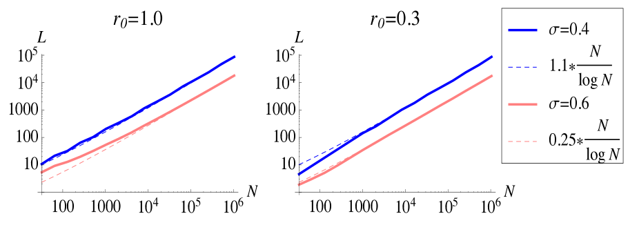
Figure 3: Memory lifetime of binary neurons is scaled close to the network size. The memory lifetime, $L$, was evaluated at two noise levels: $\sigma=0.4$ (blue solid) and $\sigma=0.6$ (red solid), and two inputs: $r_{0}=1.0$ (Left) and $r_{0}=0.3$ (Right). The offset of two curves at different noise levels reflects the different number of neurons in each layer, $n$, chosen to achieve the 90% decoding criterion. The scaling behavior was well fitted by $\sim N/\log N$ in all cases as suggested by the theoretical result.

Figure 3 plots the number of layers $L$, beyond which probability $P(\bar{r}_{L}>0|r_{0})$ falls to less than 90% at two different noise levels, $\sigma=0.4$ and $0.6$. The number of neurons in each layer, $n$, was chosen to maximize the memory lifetime under a constraint that the total number of neurons is $N$. We used two inputs, $r_{0}=1.0$ and $r_{0}=0.3$, in the simulation, but the scaling of the memory lifetime was not sensitive to the input $r_{0}$. We can see from Fig. 3 that the memory lifetime is asymptotically proportional to $N/\log N$ as predicted by the theory. Note that if the input is too small compared to the noise level ($r_{0}\ll\sigma$), the asymptotic behavior is apparent only at very large $N$ because a large number of neurons ($\gg\sigma^{2}/r_{0}^{2}$) are required to achieve the 90% reliability criterion even in the first layer.

2.3 Nonlinear dynamics provides robust working memory.

We saw in the previous section that a nearly extensive memory lifetime can be achieved by utilizing the error-correcting property of nonlinear neural dynamics. In this section, I will show that the sequential memory in this regime is much more robust to network parameters than the previously proposed solution in the semi-linear regime Ganguli et al., (2008).

To better compare the sequential memory in a nonlinear vs. semi-linear regime, let us clarify our goal. The goal is to maximize the length of the feedforward chain(s), while maintaining $I$ bits of mutual information about the input until the end of the chain(s). In this section we consider that the input, $r_{0}$, is randomly drawn from a Gaussian distribution of mean zero and variance $\sigma_{0}^{2}$. Because the information about the input can only degrade as activity propagates down the layers, it suffices to constrain the information in the final layer, i.e., the mutual information between the input and the average activity in the final layer must satisfy

$$I(r_{0};\bar{r}_{L})\geq I.$$ (15)

Let us now review the sequential memory in the semi-linear regime Ganguli et al., (2008). The feedforward network structure in this setting is similar to the one used in this paper except that the number of neurons in each layer, $n_{l}$ for layer $l$, can vary. The total number of neurons is given by $N=\sum_{l=1}^{L}n_{l}$. The derivation of Eqs. 3 and 2.1 is analogous with the variable number of neurons in each layer. When the activity is small, the conditional mean of Eq. 2.1 is well approximated by a linear function with slope (gain) $\mu^{\prime}(0)$. As previously explained, if the gain is smaller than 1, the signal tends to decay toward zero, and if the gain is larger than 1, the signal tends to grow until nonlinearity eventually kicks in (c.f. Fig. 2). The optimal semi-linear solution is achieved by setting the gain equal to 1 so that the signal neither decays nor grows on average, and memory only degrades due to fluctuation of the activity. In this case, the memory lifetime can scale with $\sqrt{N}$ Ganguli et al., (2008). To implement this semi-linear solution, however, some fine-tuning is required. For example, Ganguli et al. simply used $\phi(x)=\tanh(x)$ without explicitly considering the effect of noise that reduces the gain Herrmann et al., (1995). Because the slope of $\phi(x)=\tanh(x)$ is always less than 1 except at the origin, the gain must be strictly less than 1 in the presence of noise ($\mu^{\prime}(0)=\int D\xi\phi^{\prime}(\sigma\xi)<1$). This means that the signal must decay at each time step by the factor $\mu^{\prime}(0)<1$, and because the gain is independent of the number of neurons, the memory lifetime is indeed order 1 rather than $\sqrt{N}$. To implement the memory lifetime of $\sim\sqrt{N}$, one needs to fine-tune parameters such as the slope $\beta$ of nonlinearity $\phi(x)=\tanh(\beta x)$. The solution of $\beta$ that yields $\mu^{\prime}(0)=1$ deviates from $\beta=1$ as the noise level increases, and this difference becomes apparent at large $N$. One should also note that the fine-tuning of the slope, $\beta$, only provides a linear relation locally at around zero activity ($\bar{r}\approx 0$). If the activity is large in magnitude, the signal tends to decay due to nonlinear effects.

Suppose we fine-tuned the gain to 1 and assumed the linear input-output relation (which is not true if the signal and/or noise is large). It is easy then to estimate the mutual information between input and output because $P(\bar{r}_{L}|r_{0})$ is approximately Gaussian. The signal-to-noise ratio in the final layer is described by $\sigma_{0}^{2}/(\sum_{l=1}^{L}\sigma^{2}/n_{l})$, where the signal is preserved by setting the gain equal to 1, and the noise of variance $\sigma^{2}/n_{l}$ is added in each layer. Hence, under this semi-linear scheme, the mutual information is

$$I(r_{0};\bar{r}_{L}) = \frac{1}{2}\log_{2}\left[1+\frac{\sigma_{0}^{2}}{L\sigma^{2}}\left(\frac{1}{L}\sum_{l=1}^{L}\frac{1}{n_{l}}\right)^{-1}\right]$$ (16)

$$\leq \frac{1}{2}\log_{2}\left[1+\frac{\sigma_{0}^{2}}{L\sigma^{2}}\left(\frac{1}{\frac{1}{L}\sum_{l=1}^{L}n_{l}}\right)^{-1}\right]$$

$$= \frac{1}{2}\log_{2}\left[1+\frac{N\sigma_{0}^{2}}{L^{2}\sigma^{2}}\right],$$

where the second line follows due to the convexity of the $1/x$ function, and the equality holds if and only if the number of neurons in each layer is uniform ($n_{l}=N/L$ for all $l$) Lim and Goldman, (2011). Hence, the best achievable memory lifetime that guarantees $I$ bits of information about input under this semi-linear scheme is

$$L=\min\left(\frac{\sigma_{0}}{\sigma}\sqrt{\frac{N}{2^{2I}-1}},N\right),$$ (17)

where $\min$ takes the minimum argument. This means that unless the number of neurons is small, i.e., $N<(\sigma_{0}^{2}/\sigma^{2})/(2^{2I}-1)$, the memory lifetime of the semi-linear network is proportional to $\sqrt{N}$ and exponentially decreases with $I$, suggesting that it is difficult to maintain precise information about input in this setting. If a large amount of information is required, however, we can apply the parallel scheme used in Sec. 2.1 to the semi-linear memory by dividing $N$ neurons to $k$ parallel chains, where each chain consists of $N/k$ neurons. Provided there is independent input to each chain, a single chain only needs to retain $I/k$ bits of information in the final layers. Hence, the memory lifetime of the semi-linear parallel chains becomes

$$L=\min\left(\frac{\sigma_{0}}{\sigma}\sqrt{\frac{(N/k)}{2^{2I/k}-1}},\frac{N}{k}\right).$$ (18)

In Eq. 18, the first and second arguments of $\min(\cdot)$ are increasing and decreasing functions of $k$, respectively. Hence, the best memory lifetime for large $N$ is given by

$$L\approx\frac{\sigma_{0}}{\sigma}\sqrt{\frac{N}{(2\log 2)I}}$$ (19)

at $k\approx(\sigma/\sigma_{0})\sqrt{(2\log 2)NI}$, where each chain needs to retain much less information than the single chain scheme. Although the use of parallel chains does not alter the asymptotic scaling of memory lifetime to $N$, it is also beneficial in the semi-linear regime to buffer a large amount of information. Comparing the memory lifetime in two regimes, $\sim(N/I)\log(N/I)$ in the nonlinear regime and $\sim\sqrt{N/I}$ in the semi-linear regime, we can conclude that the memory lifetime to retain the same amount of information increases asymptotically faster with $N$ in the nonlinear regime than in the semi-linear regime.

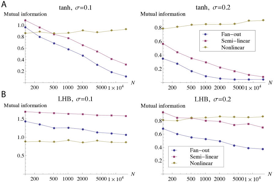
Figure 4: The nonlinear network outperformed the semi-linear network for large network sizes or with large noise. A Gaussian random input with zero mean and standard deviation $\sigma_{0}=0.5$ was provided to the first layer, and the performance was measured by the mutual information of the input and the activity in the final layer. The sequential memory performance was numerically examined at noise level $\sigma$, shown in each panel and with two nonlinear functions: (A) the hyperbolic tangent nonlinearity $\phi(x)=\tanh(\beta x)$ and (B) a piecewise-linear function $\phi(x)=\beta x$ for $|x|<1/\beta$ with hard saturating bounds (LHB). Three types of networks were compared with approximately the same size, $N$, and the same number of layers $L\approx\sqrt{2N}$ for a fair comparison: the fan-out network Ganguli et al., (2008) with $\beta=1$ and a linearly increasing number of neurons along deeper layers ($n_{l}=l$; order 1 memory lifetime); the semi-linear network with a $\beta$ solution that yielded a gain equal to 1 and a fixed number of neurons in each layer ($n_{l}=N/L$; order $\sqrt{N}$ memory lifetime); and the nonlinear network with the same network architecture as the semi-linear network but with $\beta=2$ ($n_{l}=N/L$, order $N/\log N$ memory lifetime). The semi-linear network always showed better performance than the fan-out network and the nonlinear network was superior to the other two except at a small network size and with a small amount of noise.

In practice, the network size $N$ is always finite. Hence, whether we see the differences in the order 1, $\sqrt{N}$, and $N/\log N$ memory lifetimes depends on the network size. I therefore investigated three different networks with about the same number of total neurons $N$ and the same number of layers $L$: the fan-out network Ganguli et al., (2008) with a linearly increasing number of neurons along layers ($n_{l}=l$) and $\beta=1$; the semi-linear network with a fixed number of neurons in each layer and a $\beta$ solution that yielded a gain equal to 1; and the nonlinear network, which had the same network architecture as the semi-linear network, but with $\beta=2$ (and a gain greater than 1). For a fair comparison, the number of neurons per layer was adjusted for the semi-linear and nonlinear networks so that the total number of neurons was approximately the same as that of the fan-out network, i.e., $N=L(L+1)/2$. Figure 4A shows the mutual information between the Gaussian input and the activity in the final layer for the three networks introduced above for various network sizes with $\phi(x)=\tanh(\beta x)$. When noise was small ($\sigma=0.1$), the performance of the semi-linear and fan-out networks was superior to that of the non-linear network with a small network size. This was because the nonlinear network squashed the analog inputs to almost binary values, reducing information down to about one bit, but the fan-out and semi-linear networks were able to retain more than one bit of information at a small network size and with low noise. As expected, the semi-linear network preserved more information than the fan-out network because of the fine-tuning of $\beta$ and the optimal network architecture. When the network size was larger than 500, the nonlinear network preserved more information than the other networks. At a slightly higher noise level ($\sigma=0.2$), the nonlinear network always outperformed the other two in the range of network sizes examined. Note that the mutual information of the nonlinear network increased with the network size here because the number of layers was matched to the fan-out network. This means that the nonlinear chain can be significantly longer than the fan-out and semi-linear chains to achieve a comparable level of mutual information. Figure 4B shows results analogous to Fig. 4A but using for $\phi$ a linear function with hard saturating bounds (LHB), i.e., $\phi(x)=\mbox{sgn}(x)\min(|\beta x|,1)$. The results were qualitatively similar to Fig. 4A but the fan-out and semi-linear networks performed better in this figure because LHB retained linearity for a larger range of input than the hyperbolic tangent function. In particular, compared at the same noise levels, the crossover point of the semi-linear and nonlinear networks with LHB nonlinearity lay at a larger $N$ than with the tangent hyperbolic nonlinearity. Because the nonlinear functions used in 4A and 4B share the same slope at the origin, the result shows that not only $N$ and $\sigma$, but also the nonlinearity affects the crossover point of the semi-linear and nonlinear networks.

We should also note that when more biological neuron models are used, it is even more difficult for the semi-linear model to set the gain equal to 1 because the nonlinearity is not fixed but changes with the dynamical input properties in those models. Hence, the semi-linear memory requires some elaborate additional mechanism to achieve full performance. Another important and potentially testable difference between the semi-linear and non-linear memory is how the memory lifetime, $L$, scales with the variance, $v$, of the network activity, i.e., $L\sim v^{-\gamma}$ with some exponent $\gamma$. While the semi-linear memory provides $\gamma=1/2$ from Eq. 18, the non-linear memory provides $\gamma=1$ from Eq. 11.

2.4 Synfire chains can reliably buffer complex spike sequences of leaky integrate-and-fire neurons.

The abstract firing rate model studied in the previous sections was suitable for mathematical analyses but was less biologically realistic. However, all the main properties explored in the previous sections should hold even with more realistic models. The key properties that yielded the nearly extensive sequential memory lifetime were the feedforward propagation of activity (that prevents stimuli presented at different timings from mixing) and the attracting dynamics (that implements error-correction). To illustrate this point, a feedforward network of leaky integrate-and-fire (LIF) neurons was explored. Detailed parameter studies were, however, not the scope of this paper.

A network of $N=4000$ current-based LIF neurons was simulated, e.g., Dayan and Abbott, (2001); Vogels and Abbott, (2005). The network consists of $k=10$ independent synfire chains, where each chain has $L=20$ layers and $n=20$ neurons in each layer. The membrane dynamics of neurons $i\,(i=1,2,\dots,N)$ is described by

$$\tau\frac{dV_{i}}{dt}(t)=-V_{i}(t)+E_{L}+x_{i}(t)+\mu_{bg}+\sigma_{bg}\xi_{i}(t),$$ (20)

where $V_{i}$ is the membrane potential of neuron $i$, $\tau=10$ ms is the membrane time-constant, $E_{L}=-70$ mV is the resting potential, $x_{i}$ is the input to neuron $i$ from other neurons in a local network, $\mu_{bg}=7$ mV is the mean background input level, $\xi_{i}$ is white Gaussian noise of unit variance, and $\sigma_{bg}=5$ mV describes the magnitude of background input fluctuation. When the membrane potential reaches the threshold value of $V_{th}=-50$ mV, the neuron emits a spike and the membrane potential is reset to $V_{reset}=-70$ mV. After the spike, the membrane potential is fixed at $V_{rest}$ for the duration of the refractory period, $\tau_{ref}=2$ ms. Input to neuron $i$ is calculated according to

$$\tau_{x}\frac{dx_{i}}{dt}(t)=-x_{i}(t)+\sum_{j=1}^{N}\sum_{f}w_{ij}\delta(t-t_{j}^{(f)})$$ (21)

where $\tau_{x}=5$ ms, $w_{ij}$ is the synaptic strength from neuron $j$ to $i$, $\delta(t)$ is the Dirac delta function, and $t_{j}^{(f)}$ is the $f$th spike time of neuron $j$. This means that when neuron $i$ receives a spike from neuron $j$ at $t_{j}^{(f)}$, its membrane potential is depolarized by $w_{ij}[e^{-(t-t_{j}^{(f)})/\tau}-e^{-(t-t_{j}^{(f)})/\tau_{x}}]/(\tau-\tau_{x})$ for $t>t_{j}^{(t)}$. We measure the synaptic strength $w_{ij}$ using the peak amplitude of the excitatory postsynaptic potential, which is about $w_{ij}*50\,\mbox{s}^{-1}$ for the current set of parameters. The synaptic strength, $w_{ij}$, takes a uniform non-zero value, $w$, if the layer of neuron $i$ is next to the layer of neuron $j$, and takes zero otherwise. The feedforward synaptic strength between adjacent layers is set uniformly to $1.0$ mV except in Fig. 5C, where $w$ is varied as a control parameter. Each chain is independently stimulated by $10$-Hz random Poisson pulses, upon which all the neurons in the first layer are depolarized by $10$ mV according to the time course of excitatory synaptic input.

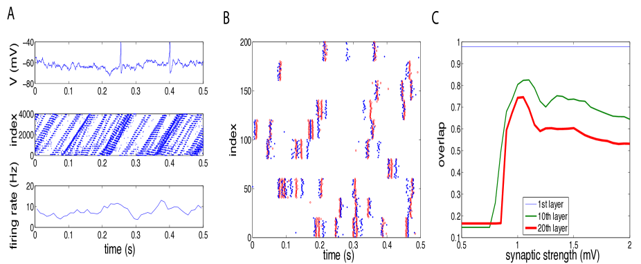
Figure 5: A feedforward network of leaky integrate-and-fire neurons reliably buffered spike patterns. (A) Top: Membrane potential of a single neuron. Middle: Spike-timing of all neurons in the network. The network consisted of $k=10$ independent synfire chains, where each synfire chain had $L=20$ layers and $n=20$ neurons in each layer. The oblique patterns describe feedforward propagation of synfire activity. Bottom: The population firing rate of all the neurons averaged in 10-ms bins. (B) The spiking pattern of the first layers (blue dots) was well preserved even until the final 20th layers (red circles). The spike pattern of the final layers was shifted so that the spike overlap with the first layers was maximized. The feedforward synaptic strengths were set to 1 mV. Note that input pulses were somewhat degraded by background noise even in the first layer. (C) The spike overlap with the input pulses in the 1st, 10th, and 20th layers plotted for different feedforward synaptic strengths.

Figure 5A shows the model behavior. The top panel shows the membrane potential of a single neuron. The middle panel shows the spiking pattern of all neurons, where neurons were indexed first within the same layer of the same chain, then across chains, and finally across layers. The oblique arrangements of spiking patterns in the middle panel demonstrates that most of the synchronous firing patters evoked by external input pulses successfully reached the final layers in about 100 ms. The bottom panel shows that the overall population firing rate of the network was kept at about 10 Hz. Figure 5B shows the spike patterns of the first and last layers. To better show the similarity, the spike time of the last layers was temporally shifted so that the spiking activity in these two layers could be viewed closer together. The figure demonstrates that the precise spike pattern was well preserved even until the final layers. To quantify the similarity of two spike trains (sums of Dirac delta functions) $S_{1}(t)$ and $S_{2}(t)$, we define the inner product $\langle S_{1},S_{2}\rangle=\int_{0}^{T}\int_{0}^{T}S_{1}(t)D(t-t^{\prime})s_{2}(t^{\prime})dtdt^{\prime}$, using the entire duration of simulations, $T$, and a smoothing kernel $D(t)=\exp(-t^{2}/(2\tau_{D}^{2}))/\sqrt{2\pi\tau_{D}^{2}}$ with $\tau_{D}=10$ ms. The overlap of the two spike trains are then measured, using the correlation coefficient, by $\langle S_{1},S_{2}\rangle/\sqrt{\langle S_{1},S_{1}\rangle\langle S_{2},S_{2}\rangle}$. The overlap of the external input pulses and the spiking activity in different layers are compared more systematically in Fig. 5C for various values of the feedforward synaptic strengths, $w$. Note that the amplitude of external input pulses to the first layers of the chains was always fixed at 10 mV. The key parameter for the signal propagation was the effective input amplitude, $nw$, which is the product of synaptic strengths and the number of neurons in each layer. When this effective coupling strength was too small, the activity could not be successfully propagated to the next layers, and when the effective coupling strength was too strong, even a spontaneous firing of a single neuron was sufficient to activate most of the neurons in the next layer. For the network structure explored here, the best overlap was achieved using about 1 mV of feedforward synaptic strength. The figure suggests that the fine-tuning of the synaptic strength is not critical for the memory lifetime because the difference between the overlaps in the 10th and 20th layers did not expand rapidly as mistuning from the optimal parameter value increased.

3 Discussion

I estimated the memory lifetime achieved by coupled nonlinear neurons. In contrast to the previously proposed semi-linear scheme that provided the order $\sqrt{N}$ memory lifetime Ganguli et al., (2008), I have shown that an order $N/\log N$ memory lifetime can be achieved by appropriately using nonlinear dynamics. The derived asymptotic scaling was invariant to the accuracy of the information buffered. The proposed nonlinear network outperformed a previously proposed semi-linear scheme in a wide range of parameters, in particular, with a large number of neurons and large noise. I have also demonstrated that the previously proposed semi-linear scheme is sensitive to the noise level, i.e., a small increase in the noise level causes monotonic decay of the average activity, turning the order $\sqrt{N}$ memory lifetime to order $1$. The nonlinear scheme proposed in this paper, on the other hand, uses large gain to prevent the activity from decaying and to alleviate the accumulation of noise using error-correcting nonlinear dynamics. Because the mathematical model studied here is general, the result that a network is capable of buffering sequential input much longer than individual elements is potentially applicable to other systems beyond neural networks, such as, gene/protein and social networks.

We considered in this paper the sequential memory task that aims to reconstruct a whole dynamical sequence of input after some delay. Note that this task is different from delayed matching working memory tasks Fuster, (1973); Goldman-Rakic, (1995), where a brief stimulus is presented only at a certain time. The major difference is that stimuli presented at different timings can interfere with each other under the sequential memory task. This typically happens when recurrently connected networks are used to buffer a sequence of input Büsing et al., (2010); Lim and Goldman, (2011). For example, under the sequence generations by Hopfield-type networks Hopfield, (1982); Sompolinsky and Kanter, (1986); Kleinfeld, (1986) or by winnerless competition networks Seliger et al., (2003); Bick and Rabinovich, (2009), the activity converges to one of the learned patterns, and the presentation of a new pattern disrupts the current state. Hence, the delay-line structure is often considered for a sequential memory task to prevent the interference of signals presented at different timings Ganguli et al., (2008). While nonlinear attracting dynamics has been utilized for non-sequential working memory tasks Camperi and Wang, (1998); Lisman et al., (1998); Koulakov, (2001); Goldman et al., (2003), this study shows that its error-correcting property also provides long-lasting memory for a sequential memory task with a feed-forward network architecture.

The feedforward network structure presented in this paper was studied in the context of synfire chains Abeles, (1991); Aertsen et al., (1996); Diesmann et al., (1999); Rossum et al., (2002); Vogels and Abbott, (2005); Kumar et al., (2008), where precise temporal patterns of spikes are their prominent characteristic. Temporally precise spiking patterns have been observed across different brain areas and different recording conditions Takahashi et al., (2010); Hahnloser et al., (2002); Pastalkova et al., (2008); Ji and Wilson, (2007); Ikegaya et al., (2004); Jin et al., (2007). There is also some experimental evidence suggesting that the synfire chain is the underlying network architecture in the brain for generating precise temporal sequences Long et al., (2010). Although the effect of noise on the gain was systematically studied Herrmann et al., (1995), the contribution of occasional large noise that blocks or spontaneously ignites synfire activity Bienenstock, (1995); Tetzlaff et al., (2002) was not theoretically analyzed. In particular, the trade-off between the length of the chain and the reliability of activity being propagated for a fixed total number of neurons was not elucidated. I demonstrated that such occasional large noise prevents synfire chains from achieving an extensive memory lifetime, and the resulting $\sim N/\log N$ memory lifetime is the direct consequence of such noise.

Reservoir computing Jaeger and Haas, (2004); Maass et al., (2002) was recently proposed as an attractive paradigm for universal and dynamical computation. This is one candidate network that can also perform sequential memory tasks White et al., (2004). According to this paradigm, dynamical input is provided to a pool of neurons, called a reservoir, which buffers the history of the input and extracts many useful features of the input sequence. Some linear readout units are placed on top of this reservoir and trained for a specific task, for example for reconstructing past input, while the reservoir itself remains task-nonspecific. One of the fundamental aspects of reservoir computing is that a reservoir buffers past input sequences so that the readout unit can successfully combine the history of the input stimuli. Although randomly connected networks are commonly used as the reservoir, the optimal structure of the reservoir is not yet known Lazar et al., (2009). The current study has shown that a feedforward structure is suitable to buffer sequences of events. Despite its benefit for sequential memory, making the whole network into a feedforward network is probably not a good idea. In addition to memory, it is also important for the reservoir to map input to a high dimensional “feature space” so that a linear readout has access to useful features Jaeger and Haas, (2004); Maass et al., (2002); Sussillo and Abbott, (2009); Bertschinger and Natschläger, (2004); Büsing et al., (2010). The current study suggests instead that it would be a promising approach to embed feedforward chains with high gain as a memory-specific sub-network for a wide class of tasks that requires a long-lasting sequential memory. This guarantees a memory lifetime that is nearly proportional to the size of that memory-specific sub-network. We should note that a straightforward implementation of randomly and recurrently connected nonlinear neurons only achieved a memory lifetime of order $\log N$ Büsing et al., (2010). In view of the fact that the best possible scaling of memory lifetime is $\sim N$ for non-sparse input sequences Ganguli and Sompolinsky, (2010), it is clear that the error-correcting feedforward network studied in this paper with $\sim N/\log N$ memory lifetime is a promising candidate for general dynamical computations requiring a recent history of activity.

References

- Abeles, (1982) Abeles, M. (1982). Local Cortical Circuits: An Electrophysiological study. Springer, Berlin.
- Abeles, (1991) Abeles, M. (1991). Corticonics. Cambridge Univ Pr, Cambridge.
- Aertsen et al., (1996) Aertsen, A., Diesmann, M., and Gewaltig, M. (1996). propagation of synchronous spiking activity in feedforward neural networks. Journal of Physiology-Paris, 90(3-4):243–247.
- Baddeley, (2000) Baddeley, A. (2000). The episodic buffer: a new component of working memory? Trends in cognitive sciences, 4(11):417–423.
- Baeg et al., (2003) Baeg, E., Kim, Y., Huh, K., Mook-Jung, I., Kim, H., and Jung, M. (2003). Dynamics of population code for working memory in the prefrontal cortex. Neuron, 40(1):177–188.
- Bertschinger and Natschläger, (2004) Bertschinger, N. and Natschläger, T. (2004). Real-Time Computation at the Edge of Chaos in Recurrent. Neural Computation, 1436:1413–1436.
- Bick and Rabinovich, (2009) Bick, C. and Rabinovich, M. I. (2009). Dynamical Origin of the Effective Storage Capacity in the Brain Working Memory. Physical Review Letters, 103(21):1–4.
- Bienenstock, (1995) Bienenstock, E. (1995). A model of neocortex. Network: Computation in Neural Systems, 6(2):179–224.
- Büsing et al., (2010) Büsing, L., Schrauwen, B., and Legenstein, R. (2010). Connectivity, Dynamics, andMemory in Reservoir Computing with Binary and Analog Neurons. Neural computation, 22(5):1272–1311.
- Camperi and Wang, (1998) Camperi, M. and Wang, X. J. (1998). A model of visuospatial working memory in prefrontal cortex: recurrent network and cellular bistability. Journal of Computational Neuroscience, 5(4):383–405.
- Dayan and Abbott, (2001) Dayan, P. and Abbott, L. (2001). Theoretical neuroscience. The MIT Press, Cambridge.
- de Fockert et al., (2001) de Fockert, J. W., Rees, G., Frith, C. D., and Lavie, N. (2001). The role of working memory in visual selective attention. Science, 291(5509):1803–6.
- Diesmann et al., (1999) Diesmann, M., Gewaltig, M., and Aertsen, A. (1999). Stable propagation of synchronous spiking in cortical neural networks. Nature, 402(6761):529–533.
- Fuster, (1973) Fuster, J. (1973). Unit Activity in Prefrontal Cortex During Delayed-Response Performance: Neuronal Correlates of Transient Memory. Journal of Neurophysiology, 36(1):61–78.
- Ganguli et al., (2008) Ganguli, S., Huh, D., and Sompolinsky, H. (2008). Memory traces in dynamical systems. Proceedings of the National Academy of Sciences, 105(48):18970.
- Ganguli and Sompolinsky, (2010) Ganguli, S. and Sompolinsky, H. (2010). Short-term memory in neuronal networks through dynamical compressed sensing. In Lafferty, J., Williams, C., Shawe-Taylor, J., Zemel, R., and Culotta, A., editors, Advances in Neural Information Processing Systems 23, pages 667–675.
- Goldman, (2009) Goldman, M. S. (2009). Memory without feedback in a neural network. Neuron, 61(4):621–34.
- Goldman et al., (2003) Goldman, M. S., Levine, J. H., Major, G., Tank, D. W., and Seung, H. S. (2003). Robust Persistent Neural Activity in a Model Integrator with Multiple Hysteretic Dendrites per Neuron. Cerebral Cortex, 13(11):1185–1195.
- Goldman-Rakic, (1995) Goldman-Rakic, P. S. (1995). Cellular basis of working memory. Neuron, 14(3):477.
- Hahnloser et al., (2002) Hahnloser, R. H. R., Kozhevnikov, A. A., and Fee, M. S. (2002). An ultra-sparse code underlies the generation of neural sequences in a songbird. Nature, 797(1989):796–797.
- Herrmann et al., (1995) Herrmann, M., Hertz, J., and Prügel-Bennett, A. (1995). Analysis of synfire chains. Network: computation in neural systems, 6(3):403–414.
- Hopfield, (1982) Hopfield, J. (1982). Neural networks and physical systems with emergent collective computational abilities. Proceedings of the National Academy of Sciences of the United States of America, 79(8):2554.
- Ikegaya et al., (2004) Ikegaya, Y., Aaron, G., Cossart, R., Aronov, D., Lampl, I., Ferster, D., and Yuste, R. (2004). Synfire chains and cortical songs: temporal modules of cortical activity. Science, 304(5670):559–64.
- Jaeger and Haas, (2004) Jaeger, H. and Haas, H. (2004). Harnessing nonlinearity: Predicting chaotic systems and saving energy in wireless communication. Science, 304(5667):78.
- Ji and Wilson, (2007) Ji, D. and Wilson, M. A. (2007). Coordinated memory replay in the visual cortex and hippocampus during sleep. Nature neuroscience, 10(1):100–7.
- Jin et al., (2007) Jin, D. Z., Ramazanoglu, F. M., and Seung, H. S. (2007). Intrinsic bursting enhances the robustness of a neural network model of sequence generation by avian brain area HVC. Journal of Computational Neuroscience.
- Kleinfeld, (1986) Kleinfeld, D. (1986). Sequential state generation by model neural networks. Proceedings of the National Academy of Sciences of the United States of America, 83:9469.
- Koulakov, (2001) Koulakov, A. (2001). Properties of synaptic transmission and the global stability of delayed activity states. Network: Computation in Neural Systems, 12:47–74.
- Kumar et al., (2008) Kumar, A., Rotter, S., and Aertsen, A. (2008). Conditions for propagating synchronous spiking and asynchronous firing rates in a cortical network model. The Journal of neuroscience, 28(20):5268–80.
- Lazar et al., (2009) Lazar, A., Pipa, G., and Triesch, J. (2009). SORN: a self-organizing recurrent neural network. Frontiers in computational neuroscience, 3(October):23.
- Lim and Goldman, (2011) Lim, S. and Goldman, M. S. (2011). Noise tolerance of attractor and feedforward memory models. Neural Computation, 24(2):332-90.
- Lisman et al., (1998) Lisman, J. E., Fellous, J. M., and Wang, X. J. (1998). A role for NMDA-receptor channels in working memory. Nature neuroscience, 1(4):273–5.
- Long et al., (2010) Long, M., Jin, D., and Fee, M. (2010). Support for a synaptic chain model of neuronal sequence generation. Nature, 468(7322):394–399.
- Maass et al., (2002) Maass, W., Natschläger, T., and Markram, H. (2002). Real-time computing without stable states: A new framework for neural computation based on perturbations. Neural computation, 14(11):2531–2560.
- Münte et al., (1998) Münte, T., Schiltz, K., and Kutas, M. (1998). When temporal terms belie conceptual order. Nature, 395(6697):71–72.
- Orlov et al., (2000) Orlov, T., Yakovlev, V., and Hochstein, S., and Zohary E. (2000). Macaque monkeys categorize images by their ordinal number. Nature, 404(6773):77–80.
- Pastalkova et al., (2008) Pastalkova, E., Itskov, V., Amarasingham, A., and Buzsáki, G. (2008). Internally Generated Cell Assembly Sequences in the Rat Hippocampus. Science, 321(5894):1322.
- Risken, (1996) Risken, H. (1996). The Fokker-Planck equation, volume 18. Springer Verlag, 3rd edition.
- Rossum et al., (2002) Rossum, M. C. W. V., Turrigiano, G. G., and Nelson, S. B. (2002). Fast Propagation of Firing Rates through Layered Networks of Noisy Neurons. The Journal of neuroscience, 22(5):1956–1966.
- Seliger et al., (2003) Seliger, P., Tsimring, L., and Rabinovich, M. (2003). Dynamics-based sequential memory: Winnerless competition of patterns. Physical Review E, 67(1):1–4.
- Sompolinsky and Kanter, (1986) Sompolinsky, H. and Kanter, I. (1986). Temporal Association in Asymmetric Neural Network. Physical Review Letters, 57(22):2861.
- Sussillo and Abbott, (2009) Sussillo, D. and Abbott, L. F. (2009). Article Generating Coherent Patterns of Activity from Chaotic Neural Networks. Neuron, 63(4):544–557.
- Takahashi et al., (2010) Takahashi, N., Sasaki, T., Matsumoto, W., Matsuki, N., and Ikegaya, Y. (2010). Circuit topology for synchronizing neurons in spontaneously active networks. Proceedings of the National Academy of Sciences of the United States of America, 107(22):10244–10249.
- Tetzlaff et al., (2002) Tetzlaff, T., Geisel, T., and Diesmann, M. (2002). The ground state of cortical feed-forward networks. Neurocomputing, 44:673–678.
- Vogels and Abbott, (2005) Vogels, T. and Abbott, L. (2005). Signal propagation and logic gating in networks of integrate-and-fire neurons. The Journal of neuroscience, 25(46):10786.
- White et al., (2004) White, O., Lee, D., and Sompolinsky, H. (2004). Short-term memory in orthogonal neural networks. Physical review letters, 92(14):148102.