EXPANDING THE TRANSFER ENTROPY TO IDENTIFY INFORMATION CIRCUITS IN COMPLEX SYSTEMS

Abstract

We propose a formal expansion of the transfer entropy to put in evidence irreducible sets of variables which provide information for the future state of each assigned target. Multiplets characterized by a large contribution to the expansion are associated to informational circuits present in the system, with an informational character which can be associated to the sign of the contribution. For the sake of computational complexity, we adopt the assumption of Gaussianity and use the corresponding exact formula for the conditional mutual information. We report the application of the proposed methodology on two EEG data sets.

I INTRODUCTION

The inference of couplings between dynamical subsystems, from data, is a topic of general interest. Transfer entropy te , which is related to the concept of Granger causality granger , has been proposed to distinguish effectively driving and responding elements and to detect asymmetry in the interaction of subsystems. By appropriate conditioning of transition probabilities this quantity has been shown to be superior to the standard time delayed mutual information, which fails to distinguish information that is actually exchanged from shared information due to common history and input signals lehnertz ; wibral . On the other hand, Granger formalized the notion that, if the prediction of one time series could be improved by incorporating the knowledge of past values of a second one, then the latter is said to have a causal influence on the former. Initially developed for econometric applications, Granger causality has gained popularity also in neuroscience (see, e.g., blinoska ; smirnov ; dingprl ; noiprl ; faes ). A discussion about the practical estimation of information theoretic indexes for signals of limited length can be found in porta . Transfer entropy and Granger causality are equivalent in the case of Gaussian stochastic variables barnett : they measure the information flow between variables hla . Recently it has been shown that the presence of redundant variables influences the estimate of the information flow from data, and that maximization of the total causality is connected to the detection of groups of redundant variables noired .

In recent years, information theoretic treatment of groups of correlated degrees of freedom have been used to reveal their functional roles as memory structures or those capable of processing information borst . Information theory suggests quantities that reveal if a group of variables is mutually redundant or synergetic sch ; bett . Most approaches for the identification of functional relations among nodes of a complex networks rely on the statistics of motifs, subgraphs of k nodes that appear more abundantly than expected in randomized networks with the same number of nodes and degree of connectivity milo ; yeger .

An interesting approach to identify functional subgraphs in complex networks, relying on an exact expansion of the mutual information with a group of variables, has been presented in bettencourt . In this work we generalize these results to show a formal expansion of the transfer entropy which puts in evidence irreducible sets of variables which provide information for the future state of the target. Multiplets of variables characterized by an high value, unjustifiable by chance, will be associated to informational circuits present in the system. Additionally, in applications where linear models are sufficient to explain the phenomenology, we propose to use the exact formula for the conditioned mutual information among Gaussian variables so as to get a computationally efficient approach. An approximate procedure is also developed, to find informational circuits of variables starting from few variables of the multiplet by means of a greedy search. We illustrate the application of the proposed expansion to a toy model and two real EEG data sets.

The paper is organized as follows. In the next section we describe the expansion and motivate our approach. In section III we report the applications of the approach and describe our greedy search algorithm. In section IV we draw our conclusions.

II Expansion

We start describing the work in bettencourt . Given a stochastic variable $X$ and a family of stochastic variables $\{Y_{k}\}_{k=1}^{n}$, the following expansion for the mutual information, analogous to a Taylor series, has been derived there:

$$\begin{array}[]{l}S\left(X|\{Y\}\right)-S(X)=-I\left(X;\{Y\}\right)=\\ \sum_{i}{\Delta S(X)\over\Delta Y_{i}}+\sum_{i>j}{\Delta^{2}S(X)\over\Delta Y_{i}\Delta Y_{j}}+\cdots+{\Delta^{n}S(X)\over\Delta Y_{i}\cdots\Delta Y_{n}},\\ \end{array}$$ (3)

where the variational operators are defined as

$${\Delta S(X)\over\Delta Y_{i}}=S\left(X|Y_{i}\right)-S(X)=-I\left(X;Y_{i}\right),$$ (4)

$${\Delta^{2}S(X)\over\Delta Y_{i}\Delta Y_{j}}=-{\Delta I\left(X;Y_{i}\right)\over\Delta Y_{j}}=I\left(X;Y_{i}\right)-I\left(X;Y_{i}\right|Y_{j}),$$ (5)

$${\Delta^{3}S(X)\over\Delta Y_{i}\Delta Y_{j}\Delta Y_{k}}=I\left(X;Y_{i}|Y_{k}\right)-I\left(X;Y_{i}\right|Y_{j},Y_{k})-I\left(X;Y_{i}\right)+I\left(X;Y_{i}\right|Y_{j}),$$ (6)

and so on.

Now, let us consider $n+1$ time series $\{x_{\alpha}(t)\}_{\alpha=0,\ldots,n}$. The lagged state vectors are denoted

$$Y_{\alpha}(t)=\left(x_{\alpha}(t-m),\ldots,x_{\alpha}(t-1)\right),$$

$m$ being the window length.

Firstly we may use the expansion (3) to model the statistical dependencies among the $x$ variables at equal times. We take $x_{0}$ as the target time series, and the first terms of the expansion are

$$W_{i}^{0}=-I\left(x_{0};x_{i}\right)$$ (7)

for the first order;

$$Z_{ij}^{0}=I\left(x_{0};x_{i}\right)-I\left(x_{0};x_{i}|x_{j}\right)$$ (8)

for the second order; and so on. We note that

$$Z_{ij}^{0}=-{\cal I}\left(x_{0};x_{i};x_{j}\right),$$

where ${\cal I}\left(x_{0};x_{i};x_{j}\right)$ is the interaction information, a well known information measure for sets of three variables mcgill ; it expresses the amount of information (redundancy or synergy) bound up in a set of variables, beyond that which is present in any subset of those variables. Unlike the mutual information, the interaction information can be either positive or negative. Common-cause structures lead to negative interaction information . As a typical example of positive interaction information one may consider the three variables of the following system: the output of an XOR gate with two independent random inputs (however some difficulties may arise in the interpretation of the interaction information, see bell ). It follows that positive (negative) $Z_{ij}^{0}$ corresponds to redundancy (synergy) among the three variables $x_{0}$, $x_{i}$ and $x_{j}$.

In order to go beyond equal time correlations, here we propose to consider the flow of information from multiplets of variables to a given target. Accordingly, we consider

$$S\left(x_{0}|\{Y_{k}\}_{k=1}^{n}\right)-S(x_{0})=-I\left(x_{0};\{Y_{k}\}_{k=1}^{n}\right),$$ (9)

which measures to what extent all the remaining variables contribute to specifying the future state of $x_{0}$. This quantity can be expanded according to (3):

$$\begin{array}[]{l}S\left(x_{0}|\{Y_{k}\}_{k=1}^{n}\right)-S(x_{0})=\\ \sum_{i}{\Delta S(x_{0})\over\Delta Y_{i}}+\sum_{i>j}{\Delta^{2}S(x_{0})\over\Delta Y_{i}\Delta Y_{j}}+\cdots+{\Delta^{n}S(x_{0})\over\Delta Y_{i}\cdots\Delta Y_{n}}.\\ \end{array}$$ (12)

A drawback of the expansion (9) is that it does not remove shared information due to common history and input signals; therefore we choose to condition it on the past of $x_{0}$, i.e. $Y_{0}$. To this aim we introduce the conditioning operator ${\cal C}_{Y_{0}}$:

$${\cal C}_{Y_{0}}S(X)=S(X|Y_{0}),$$

and observe that ${\cal C}_{Y_{0}}$ and the variational operators (4) commute. It follows that we can condition the expansion (12) term by term, thus obtaining

$$\begin{array}[]{l}S\left(x_{0}|\{Y_{k}\}_{k=1}^{n},Y_{0}\right)-S(x_{0}|Y_{0})=-I\left(x_{0};\{Y\}_{k=1}^{n}|Y_{0}\right)=\\ \sum_{i}{\Delta S(x_{0}|Y_{0})\over\Delta Y_{i}}+\sum_{i>j}{\Delta^{2}S(x_{0}|Y_{0})\over\Delta Y_{i}\Delta Y_{j}}+\cdots+{\Delta^{n}S(x_{0}|Y_{0})\over\Delta Y_{i}\cdots\Delta Y_{n}}.\\ \end{array}$$ (15)

The first order terms in the expansion are given by:

$$A_{i}^{0}={\Delta S(x_{0}|Y_{0})\over\Delta Y_{i}}=-I\left(x_{0};Y_{i}|Y_{0}\right),$$ (16)

and coincide with the bivariate transfer entropies $i\to 0$ (times -1). The second order terms are

$$B_{ij}^{0}=I\left(x_{0};Y_{i}|Y_{0}\right)-I\left(x_{0};Y_{i}|Y_{j},Y_{0}\right),$$ (17)

and may be seen as a generalization of the interaction information ${\cal I}$; hence a positive (negative) $B_{ij}^{0}$ corresponds to a redundant (synergetic) flow of information $\{i,j\}\to 0$. The typical examples of synergy and redundancy, in the present framework of network analysis, are the same as in the static case, plus a delay for the flow of information towards the target. The third order terms are

$$\begin{array}[]{ll}C_{ijk}^{0}=&I\left(x_{0};Y_{i}|Y_{j},Y_{0}\right)+I\left(x_{0};Y_{i}|Y_{k},Y_{0}\right)\\ &-I\left(x_{0};Y_{i}|Y_{0}\right)-I\left(x_{0};Y_{i}|Y_{j},Y_{k},Y_{0}\right),\end{array}$$ (20)

and so on.

The generic term in the expansion (15),

$$\Omega_{k}={\Delta^{k}S(x_{0}|Y_{0})\over\Delta Y_{i}\cdots\Delta Y_{k}},$$ (21)

is symmetrical under permutations of the $Y_{i}$ and, remarkably, statistical independence among any of the $Y_{i}$ results in vanishing contribution to that order. Therefore each nonvanishing accounts for an irreducible set of variables providing information for the specification of the target: the search for for informational multiplets is thus equivalent to search for terms (21) which are significantly different from zero. Another property of (15) is that the sign of each term is connected to the informational character of the corresponding set of variables, see bettencourt ).

For practical applications, a reliable estimate of conditional mutual information from data should be used. Non parametric methods are recommendable when nonlinear effects are relevant. However, a conspicuous amount of phenomenology in brain can be explained by linear models: therefore, for the sake of computational load, In this work we adopt the assumption of Gaussianity and use the exact expression that holds in this case barnett , which reads as follows. Given multivariate Gaussian random variables $X$, $W$ and $Z$, the conditioned mutual information is

$$I\left(X;W|Z\right)=\frac{1}{2}\ln{|\Sigma(X|Z)|\over|\Sigma(X|W\oplus Z)|},$$ (22)

where $|\cdot|$ denotes the determinant, and the partial covariance matrix is defined

$$\Sigma(X|Z)=\Sigma(X)-\Sigma(X,Z)\Sigma(Z)^{-1}\Sigma(X,Z)^{\top},$$ (23)

in terms of the covariance matrix $\Sigma(X)$ and the cross covariance matrix $\Sigma(X,Z)$; the definition of $\Sigma(X|W\oplus Z)$ is analogous.

The statistical significance of (21) can be assessed by observing that it is the sum of terms like (22) which, under the null hypothesis $I\left(X;W|Z\right)=0$, have a $\chi^{2}$ distribution. Alternatively, statistical testing may be done using surrogate data obtained by random temporal shuffling of the target vector $x_{0}$; the latter strategy is the one we use in this work.

III APPLICATIONS

III.1 Second order terms

In this subsection we show the application of the proposed expansion, truncated at the second order. To this aim we turn to real electroencephalogram (EEG) data, the window length $m$ being fixed by cross validation. Firstly we consider recordings obtained at rest from 10 healthy subjects. During the experiment, which lasted for 15 min, the subjects were instructed to relax and keep their eyes closed. To avoid drowsiness, every minute the subjects were asked to open their eyes for 5 s. EEG was measured with a standard 10-20 system consisting of 19 channels nolte . Data were analyzed using the linked mastoids reference, and are available from website_nolte .

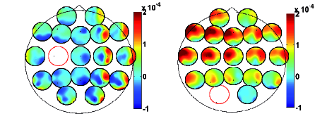
Figure 2: The lagged components $B^{0}_{ij}$ for two target electrodes, C3 on the left and O1 on the right. The target electrode is in white, and for each of the other electrodes $i$ on the map, the value of $B^{0}_{ij}$ is displayed for the other electrodes.

For each subject we consider several epochs of 4 seconds in which the subjects kept their eyes closed. For each epoch we compute the second order terms at equal times $Z^{0}_{ij}$ and the lagged ones $B^{0}_{ij}$; then we average the results over epochs. In order to visualize these results, for each target electrode we plot a on a topographic scalp map the pairs of electrodes which are redundant or synergetic with respect to it. Both quantities are distributed with a clear pattern across the scalp. Interactions at equal times are one order of magnitude higher than the lagged interactions, and are dominated by the effect of spatial proximity, see fig. 1. On the other hand, $B^{0}_{ij}$ show a richer dynamics, such as interhemispheric communications and predominance redundancy to and from the occipital channels, see fig. 2, reflecting the prominence of the occipital rhythms when the subjects rest with their eyes closed.

As another example we consider intracranial EEG recordings from a patient with drug-resistant epilepsy and which has thus been implanted with an array of $8\times 8$ cortical electrodes and two depth electrodes with six contacts. The data are available at kol_web and described in kol_paper . For each seizure data are recorded from the preictal period, the 10 seconds preceding the clinical onset of the seizure, and the ictal period, 10 seconds from the clinical onset of the seizure. We analyze data corresponding to eight seizures and average the corresponding results.

For each electrode we compute the lagged influences $B^{0}_{ij}$, obtaining for each electrode the pair of other electrodes with redundant or synergetic contribution to its future. The patient has a putative epileptic focus in a deep hippocampal region, with the seizure that then spreads to the cortical areas. In fig. 3 we report the values of coefficients $B$ taking as the target a cortical electrode located on the putative cortical focus: we report the values of $B^{0}_{ij}$ corresponding to all the couple of the electrodes, as well as their sum over electrode $j$. It is clear how the redundancy increases during the seizure. On the other hand, for sensors from 70 to 76, corresponding to a depth electrode, the redundancy is higher in the preictal period, reflecting the fact that the seizure is already active in its primary focus even if not yet clinically observable. The values of $B$ corresponding to this electrode are reported in fig. 4.

III.2 Greedy search of multiplets

Given a target variable, the time required for the exhaustive search of all the subsets of variables, with a statistically significant information flow (21), is exponential in the size of the system. It follows that the exact search for large multiplets is computationally unfeasible, hence we adopt the following approximate strategy. We start from a pair of variables with non-vanishing second order term $B$ w.r.t. the given target. We consider these two variables as a seed, and aggregate other variables to them so as to construct a multiplet. The third variable of the subset is selected among the remaining ones as those that, jointly with the previously chosen variable, maximize the modulus $|C|$ of the corresponding third order term. Then, one keeps adding the rest of the variables by iterating this procedure. Calling $Z_{k-1}$ the selected set of k - 1 variables, the set $Z_{k}$ is obtained adding, to $Z_{k-1}$, the variable, among the remaining ones, with the greatest modulus of $\Omega_{k}$. These iterations stop when $\Omega_{k}$, corresponding to $Z_{k}$, is not significantly different from zero (the Bonferroni correction for multiple comparisons is to be applied at each iteration); $Z_{k-1}$ is then recognized as the multiplet originated by the initial pair of variables chosen as the seed.

We apply this strategy to the following toy model

$$\begin{array}[]{lll}x_{0}(t)&=a\;\eta(t-1)+\sigma\xi_{0}(t),&\\ x_{\alpha}(t)&=b_{\alpha}\;\eta(t)+\sigma_{1}\xi_{\alpha}(t),&\alpha=1,\ldots,m\\ x_{\beta}(t)&=\sigma_{2}\xi_{\beta}(t),&\beta=m+1,\ldots,m+M\\ \end{array}$$ (27)

where $\xi$ and $\eta$ are i.i.d. unit variance Gaussian variables. In this model the target $x_{0}$ is influenced by the process $\eta$; variables $x_{\alpha}$, $\alpha=1,\ldots,m$, are a mixture of $\eta$ and noise $\xi$, whilst the remaining $M$ variables are pure noise. Estimates of $\Omega_{k}$ are based on time series, generated from (27) and 1000 samples long. The results are displayed in figure (5). Firstly we consider the case $m=20$ and $M=0$, with all the twenty variables driving the target with equal couplings $b_{\alpha}$; in figure (5)-A we depict the term $\Omega_{k}$ corresponding to the $k$-th iteration of the greedy search. We note that $\Omega_{k}$ has alternating sign and its modulus decreases with $k$. In figure (5)-B we consider another situation, with $m=10$ and $M=10$, the ten non-zero couplings $b_{\alpha}$ being non-uniform. $\Omega_{k}$ still shows alternating sign, and $\Omega_{k}$ vanishes for $k>9$; hence the multiplet of ten variables is correctly identified. The order of selection is related to the strength of the coupling: variables with stronger coupling are selected first.

In figure (6) we consider again the EEG data from healthy subjects with closed eyes website_nolte , and apply the greedy search taking C3 as the target and $\{C4,C6\}$ as the seed. We find a subset of 9 variables influencing the target. The fact that the sign of $\Omega_{k}$ is alternating, as in the previous model, suggests that the channels in this set correspond to a single source which is responsible for the inter-hemispheric communication towards the target electrode C3. In figure (7) we take O1 as the target and $\{F3,C5\}$ as the seed. A subset of 11 variables is found which describes the information flow from the frontal to the occipital cortex.

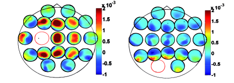
Figure 1: The instantaneous components $Z^{0}_{ij}$ for two target electrodes, C3 on the left and O1 on the right. The target electrode is in white, and for each of the other electrodes $i$ on the map, the value of $Z^{0}_{ij}$ is displayed for the other electrodes.

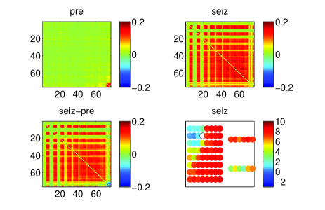
Figure 3: The lagged second order terms $B^{0}_{ij}$ for a cortical electrode (in white) right before and during the clinical onset of a seizure, and the sum over the second electrode of the pair in the lower right panel.

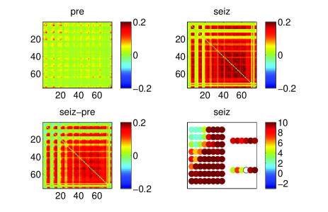
Figure 4: The lagged second order terms $B^{0}_{ij}$ for a depth electrode (in white) right before and during the clinical onset of a seizure, and the sum over the second electrode of the pair in the lower right panel.

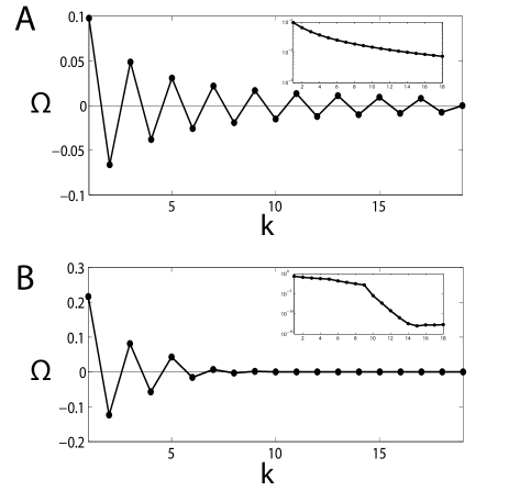
Figure 5: $\Omega_{k}$ as a function of the multiplet size $k$ for a model in which one variable is influenced by all the other variables or by part of them. In (A) $m=20$ and $M=0$: all the 20 variables influence the target with unitary weight. In (B) $m=10$ and $M=10$; the weights $b_{\alpha}$ are [ 1.75 1.75 1 1 1 1 .5 .5 .5 .5 ]. The insets show the logarithm of the absolute value of $\Omega_{k}$. The first point $k=1$, in both plots, represents the initial pair of variables chosen as the seed, i.e. $\{1,2\}$. The other parameters are, in both cases, $a,\sigma,\sigma_{1},\sigma_{2}=0.5$.

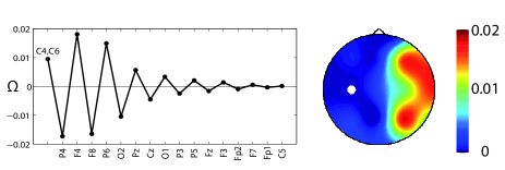
Figure 6: Informative contributions to the target electrode C3. Left: information contribute from the resulting multiplet when time series from a given electrode are added to the existing multiplet, starting from the pair (C4,C6) which is the one which shares the most of information on the future of the target time series. Channels P4, F4, F8, P6, O2, Pz and Cz are recognized to belong to the same multiplet as C4 and C6, whilst including $O1$ leads to a $\Omega_{k}$ which is not significantly different from zero. Right: the absolute value of this contributions plotted on a scalp map.

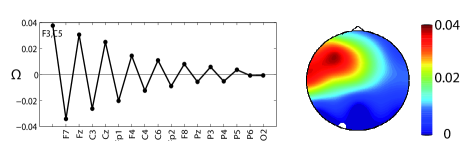
Figure 7: Informative contributions to the target electrode O1. Left: information contribute from the resulting multiplet when time series from a given electrode are added to the existing multiplet, starting from the pair (F3,C5) which is the one which shares the most of information on the future of the target time series. Nine channels (F7, Fz, C3, Cz, Fp1, F4, C4, C6, Fp2) are recognized to belong to the same multiplet, for the remaining variables $\Omega_{k}$ is not significantly different from zero. Right: the absolute value of this contributions plotted on a scalp map.

IV CONCLUSIONS

Summarizing, we have proposed to describe the flow of information, in a system, by means of multiplets of variables which send information to each assigned target node. We used a recently proposed expansion of the mutual information, between a stochastic variable and a set of other variables, to measure the character and the strength of multiplets of variables. Indeed, terms of the proposed expansion put in evidence irreducible sets of variables which provide information for the future state of the target channel. The sign of the contributions are related to their informational character; for the second order terms, synergy and redundancy correspond to negative and positive sign, respectively. For higher orders, we have shown that groups of variables, related to the same source of information, lead to contributions with alternating signs as the number of variables is increased. A decomposition with similarities to the present work have been reported in beer , where for multiple sources the distinction between unique, redundant, and synergistic transfer has been proposed; in lizier the inference of an effective network structure, given a multivariate time series, using incrementally conditioned transfer entropy measurements, has been discussed. The main purpose of this paper is to introduce an information based decomposition, and we did that in a framework unifying Granger causality and Transfer entropy, thus using a formula which is exact for linear models. In cases in which a nonlinear model is required, the entropy has to be computed, requiring a high enough number of time points for statistical validation; nonetheless the expansion that we proposed remains valid and exact in both cases.

We have reported the results of the applications to two EEG examples. The first data set is from resting brains and we found signatures of inter-hemispherical communications and frontal to occipital flow of information. Concerning a data set from an epileptic subject, our analysis puts in evidence that the seizure is already active, close to the primary lesion, before it is clinically observable.

References

- (1) T. Schreiber,Phys. Rev. Lett. 85, pp. 461-464, 2000.
- (2) C.W.J. Granger, Econometrica 37, pp. 424-438, 1969.
- (3) M. Staniek, K. Lehnertz, Phys. Rev. Lett. 100, 158101 (2008).
- (4) M. Lindner, R. Vicente, V. Priesemann, and M. Wibral, BMC Neuroscience 12, 119 (2011).
- (5) K.J. Blinowska, R. Kus, M. Kaminski, Phys. Rev. E 70, pp. 50902-50905(R), 2004.
- (6) D.A. Smirnov, B.P. Bezruchko, Phys Rev. E 79, pp. 46204-46212, 2009.
- (7) M. Dhamala, G. Rangarajan, M. Ding,Phys. Rev. Lett. 100, pp. 18701-18704, 2008.
- (8) D. Marinazzo, M. Pellicoro, S. Stramaglia, Phys. Rev. Lett. 100, pp. 144103-144107, 2008.
- (9) L. Faes, A. Porta, G. Nollo, Phys. Rev. E 78, 26201 (2008).
- (10) A. Porta et al, Methods of Information in Medicine 49, pp. 506-510, 2010.
- (11) L. Barnett, A.B. Barrett, and A.K. Seth, Phys. Rev. Lett. 103, pp. 238701-23704, 2009.
- (12) K. Hlavackova-Schindler, M. Palus, M. Vejmelka, J. Bhattacharya, Physics Reports 441, 1 (2007).
- (13) L. Angelini, M. de Tommaso, D. Marinazzo, L. Nitti, M. Pellicoro, and S. Stramaglia, Phys. Rev. E 81, 37201 (2010).
- (14) A. Borst, F.E. Theunissen, Nat. Neurosci. 2, pp. 947-957, 1999.
- (15) E. Schneidman, W. Bialek, M.J. Berry II, J. Neuroscience 23, pp. 11539-11553, 2003.
- (16) L.M.A. Bettencourt et al., Phys. Rev. E 75, pp. 21915-21924, 2007.
- (17) R. Milo et al., Science 298, pp. 824-827, 2002.
- (18) E. Yeger-Lotem et al., Proc. Natl.Acad. Sci. U.S.A. 101, pp. 5934-5939, 2004.
- (19) L.M.A. Bettencourt, V. Gintautas, M.I. Ham, Phys. Rev. Lett. 100, pp. 238701-238704, 2008.
- (20) W.J. McGill, “Multivariate information transmission” Psychometrika 19, 97-116 (1954).
- (21) A.J. Bell , “The co-information lattice”. Proceedings of ICA 2003, Nara, Japan, April 2003.
- (22) Z. Shehzad et al., Cerebral cortex 19, pp. 2209-2229, 2009.
- (23) N. Tzourio-Mazoyer et al., it Neuroimage 15, pp. 273-289, 2002.
- (24) M.D. Fox et al., Proc Natl Acad Sci U S A. 102, pp. 9673-9678, 2005.
- (25) R. Salvador et al., Cereb. Cortex 15, 1332-1342, 2005.
- (26) R. Leech, R. Braga, and D. J. Sharp, The Journal of Neuroscience 32, pp. 215-222, 2012.
- (27) G. Nolte et al., Phys. Rev. Lett. 100, pp. 234101-234104, 2008.
- (28) http://clopinet.com/causality/data/nolte/
- (29) G. Nolte, A. Ziehe, V. Nikulin, A. Schlögl, N. Krämer, T. Brismar, K.R. Müller, Phys. Rev. Lett. 100, 234101, 2008
- (30) http://clopinet.com/causality/data/nolte/, accessed may 2012
- (31) M.A. Kramer, E.D. Kolaczyk, H.E. Kirsch, Epilepsy Research 79, 173, 2008
- (32) http://math.bu.edu/people/kolaczyk/datasets.html, accessed may 2012
- (33) P.L. Williams, R.D. Beer, Generalized Measures of Information Transfer, preprint arXiv:1102.1507 (2011).
- (34) J. T. Lizier, M. Rubinov, ”Multivariate construction of effective computational networks from observational data”, preprint MPI MIS Preprint 25/2012.