Electron-phonon relaxation and excited electron distribution in zinc oxide and anatase

Abstract

We propose a first-principle method for evaluations of the time-dependent electron distribution function of excited electrons in the conduction band of semiconductors. The method takes into account the excitations of electrons by external source and the relaxation to the bottom of conduction band via electron-phonon coupling. The methods permits calculations of the non-equilibrium electron distribution function, the quasi-stationary distribution function with steady-in-time source of light, the time of setting of the quasi-stationary distribution and the time of energy loss via relaxation to the bottom of conduction band. The actual calculations have been performed for titanium dioxide in the anatase structure and zinc oxide in the wurtzite structure. We find that the quasi-stationary electron distribution function for ZnO is a fermi-like curve that rises linearly with increasing excitation energy whereas the analogous curve for anatase consists of a main peak and a shoulder. The calculations demonstrate that the relaxation of excited electrons and the setting of the quasi-stationary distribution occur within the time no more than 500 fsec for ZnO and 100 fsec for anatase. We also discuss the applicability of the effective phonon model with energy-independent electron-phonon transition probability. We find that the model only reproduces the trends in changing of the characteristic times whereas the precision of such calculations is not high. The rate of energy transfer to phonons at the quasi-stationary electron distribution also have been evaluated and the effect of this transfer on the photocatalyses has been discussed. We found that for ZnO this rate is about 5 times less than in anatase.

I Introduction

The zinc oxide in wurtzite structure and the titanium dioxide in anatase structure are the semiconductors of great interest from many viewpoints. Both demonstrate photocatalytic activity in the UV region of the sunlight spectra and are widely used as basic compounds in attempts to create the photocatalysts active in the visual sunlight that can be used for cleaning the environment from organic pollutants and pathogenic bacteria Hoff95 ; Carp04 ; Lu08 ; Ni07 ; Gird09 . They are also perspective materials for applications in solar energetics and random access memory devices Mai04 ; Kim04 ; Lane04 . The photocatalytic activity, magnetic properties and charge transport in these oxides to a great extent depend on the dynamics of the excited states, therefore in many works the characteristics of fast electron and hole dynamics have been studied. In the works Yama99 ; Hend07 ; Wen07 ; Sun05 the relaxation rates of excited electrons in ZnO via electron-phonon coupling have been estimated whereas in the papers Wata00 ; Wata01 ; Seki04 ; Hend04 the characteristics of relaxation rates for anatase have been evaluated.

The comprehension of the results obtained in the experimental works requires an application of some theoretical models that should incorporate both the conditions of experiments and the characteristics of electron dynamics determined by the properties of the solids under study. Such models have been successfully developed and widely applied for the excited electron relaxation in metals Knor02a ; Zhuk02 ; Zhuk04 . In the case of semiconductors this aim is, however, far from being achieved, partly because only recently the rigorous methods for evaluations of the characteristics of electron dynamics have been developed. The main phenomenon responsible for the relaxation of the low-energy excited electrons in semi-conductors (whose energy with respect to the bottom of the conduction band is no more than the band gap) is the electron-phonon coupling. A number of first-principle method for the calculations of the parameters of this coupling have been developed that permit to perform subsequent calculations for the temporal characteristics of electron relaxation. Possibly, the most promising of them is provided by the density-functional perturbation theory Zein84 ; Baro01 implemented in the pseudo-potential Quantum Espresso (QE) computer code. Recently this approach has been applied to the evaluations of the characteristics of electron relaxation in ZnO Zhuk10b , anatase and rutile Zhuk10a , germanium Tyut11 ,. The calculations have demonstrated a reasonable correspondence to experimental data and helped to understand some fine relations between the band structure and electron dynamics in the compounds.

The shortage of the evaluations of the Refs. Zhuk10b ; Zhuk10a was that they had been performed for a case of a single excited electron in the conduction band that falls down to the bottom of the band loosing the energy via the electron-phonon coupling. More rigorous estimations of the electron dynamics should include also the emergence of new electrons excited by the external light source and also the effect of filling the energy level under consideration with the electrons falling from the higher levels. The method of such evaluations is proposed in the current paper. Although the concrete results are obtained for ZnO and TiO₂, the proposed method does not have features preventing its application to different kinds of semi-conductors. The method is based on the fully first-principle calculations of the electron-phonon coupling constants. So it does not have simplifying assumptions on the energy dependence of the rate of electron-phonon relaxation. It is worth noting that the neglect of the energy dependence of the electron-phonon interaction is a conventional approximation, as it is e.g. with the Fröhlich’s hamiltonian DasS88 ; Tao93 ; Komi01 ; Jang07 . So, together with the characteristics of electron relaxation in ZnO and TiO₂, we discuss also the applicability of the energy-independent electron-phonon coupling and find that in the current case it is of very limited accuracy.

II Method of calculations

II.1 Quasi-stationary electron distribution

We start with the following Boltzmann equation for the time-dependent distribution function $f(t,\epsilon)$ of excited electrons (hereafter EDF) at the energy $\epsilon$ above the bottom of the conduction band of a semiconductor (hereafter - excess energy)

$$\frac{\partial f(t,\epsilon)}{\partial t}=(1-n(t,\epsilon))\int_{0}^{\omega_{m}}n(t,\epsilon+\hbar\omega)F(\epsilon+\hbar\omega,\omega)d\omega-$$ (1)

$$n(t,\epsilon)\int_{0}^{\omega_{m}}F(\epsilon,\omega)d\omega(1-n(t,\epsilon-\hbar\omega))+\frac{\partial f_{inst}(t,\epsilon)}{\partial t}$$ (2)

In this equation $n(t,\epsilon)=f(t,\epsilon)/N(\epsilon)$, where $N(\epsilon)$ is the density of electronic states, is the population of a single band state at the $\epsilon$ level. First integral describes, in a momentum-averaged manner, the process of coming of electrons to the level $\epsilon$ from all the electronic states higher by the energy $\hbar\omega$, the process accompanied by the emission of phonons whose maximum frequency is $\omega_{m}$. $F(\epsilon+\hbar\omega,\omega)$, the spectral function of electron-phonon interaction, is the probability for electrons to fall from all the band states with energy $\epsilon+\hbar\omega$ to the states at the energy $\epsilon$ emitting phonons with energy $\hbar\omega$ satisfying the conditions of energy and momentum conservation. Similarly, the second integral describes the process of electron transitions from the $\epsilon$ level to the levels lower by the phonon energy $\hbar\omega$. We discuss only the case of a small intensity of irradiation, so we assume that the $n(t,\epsilon)$ values are small and omit the factors $1-n(t,\epsilon)$. The spectral function $F(\epsilon,\omega)$, satisfying to energy and momentum conservation, has the form

$$F(\epsilon,\omega)=\sum_{{\bf qkk^{\prime}}}\sum_{nn^{\prime}\sigma}\delta(\epsilon-e_{n{\bf k}})P(n{\bf k},n^{\prime}{\bf k^{\prime}},\sigma{\bf q})\delta_{{\bf k-k^{\prime}\pm q}}\delta(\omega-\omega_{\sigma{\bf q}})\delta(\epsilon-\hbar\omega-e_{n^{\prime}{\bf k^{\prime}}})$$ (3)

where $P(n{\bf k},n^{\prime}{\bf k^{\prime}},\sigma{\bf q})$ is the probability of a single electron transition between the electronic band states $|n{\bf k}\rangle$ and $|n^{\prime}{\bf k^{\prime}}\rangle$ accompanied by the emission or absorption of the photon with frequency $\omega_{\sigma{\bf q}}$. The calculations of such spectral function, which for the Fermi level in metals is proportional to the well-known Eliashberg function, were extensively discussed in literature Maha90 ; Grim . In accordance to the ’golden Fermi rule’, this probability, per unit of time, is determined as

$$P(n{\bf k},n^{\prime}{\bf k^{\prime}},\sigma{\bf q})=(2\pi/\hbar)|\langle{n\bf k}|\Delta V_{{\bf q}\sigma}|n^{\prime}{\bf k^{\prime}}\rangle|^{2}\delta(e_{n{\bf k}}-e_{n^{\prime}{\bf k^{\prime}}})$$ (4)

Here the value $\Delta V_{{\bf q}\sigma}$ is the variation of the self-consistent potential in crystal caused by the displacement mode of the phonon, and the value $\langle{n\bf k}|\Delta V_{{\bf q}\nu}|{n^{\prime}\bf k^{\prime}}\rangle$ is the matrix element of the electron-phonon interaction. The energy of phonon, small in comparison with the energy of electronic states, is neglected here. The ways of calculating this matrix element also have been well discussed Baro01 .

The term $\partial f_{inst}(t,\epsilon)/\partial t$ in Eq. 1 describes the instantaneous electron distribution in the conduction band produced by the external source of excited electrons. One can take for this term the approximation

$$\frac{\partial f_{inst}(t,\epsilon)}{\partial t}=S_{0}(t)S(\epsilon)$$ (5)

where the factor $S_{0}(t)$, which in general can be time-dependent, is the concentration of the excited electrons determined by the power of the light radiation, and $S(\epsilon)$ is the instantaneous spectral function ( hereafter IEDF) which describes the probability for an excited electron to have the excess energy $\epsilon$. Naturally, IEDF should be normalized to unity: $\int_{0}^{\infty}S(\omega)d\omega=1$.

If one linearizes the energy dependence of the $F(\epsilon+\hbar\omega,\omega)$ with $\omega$ as a small parameter then Eq. 1 is written in the form

$$\frac{\partial f(t,\epsilon)}{\partial t}=\frac{\partial}{\partial\epsilon}[N^{-1}(\epsilon)f(t,\epsilon)B(\epsilon)]+\frac{\partial f_{inst}(t,\epsilon)}{\partial t}$$ (6)

Here the function

$$B(\epsilon)=\int_{0}^{\omega_{m}}\hbar\omega F(\epsilon,\omega)d\omega$$ (7)

is the energy lost by the electrons at the level $\epsilon$ via phonon emission. So the value which we define as $\hbar\omega_{0}=B(\epsilon)/N(\epsilon)$ is the averaged energy lost by $one$ electron in the process of phonon emission; a first-principle approach to the calculations of this value has been demonstrated in Refs. Zhuk10a ; Zhuk10b (where it has been denoted as $\Delta e$).

Eq. 6 describes the time evolution of the $f(t,\epsilon)$ EDF when the light source produces an instantaneous distribution of excited electrons in the conduction band. We discuss here the quasi-stationary case, when the temporal evolution of the external pulse is slow and $dS_{0}(t)/dt<<S_{0}(t)B(\epsilon)$. Taking $\partial f(t,\epsilon)/\partial t=0$ one has the solution of the Eq. 6 in the form

$$f(t,\epsilon)=S_{0}(t)\frac{1}{\hbar\omega_{0}}\int_{\epsilon}^{\epsilon_{m}}S(\epsilon^{\prime})d\epsilon^{\prime}$$ (8)

where $\epsilon_{m}$ is the highest excess energy of the excited electrons.

The IEDF $S(\omega)$ can be obtained from the electronic band structure calculations. Namely, if the energy of the quantum of optical excitation is $E_{exc}$, then for the excess energy $\epsilon$ one has to sum the probabilities of all direct excitations from the electronic states at the energy $\epsilon-E_{exc}$ to the states at the energy $\epsilon$. Hence, the un-normalized IEDF is

$$S(\epsilon)=\sum_{{\bf k}nn^{\prime}}\delta(\epsilon-e_{n{\bf k}})T(n{\bf k},n^{\prime}{\bf k})\delta(\epsilon-E_{exc}-e_{n^{\prime}{\bf k}})$$ (9)

where $T(n{\bf k},n^{\prime}{\bf k})$ is the probability of the transition between the states $|n{\bf k}\rangle$ and $|n^{\prime}{\bf k}\rangle$. (In practical calculations we replace the $\delta$-functions with the normalized to unity gaussians whose width at the half-maximum is 0.01 eV.) The transition probability also can be evaluated basing on the first-order perturbation theory. In order to calculate the matrix elements of the Eq. (9) we take advantage of the atomic sphere approximation Ande87 . In this approximation the integration over the space of a crystal is replaced with the integration over atomic spheres. In every atomic sphere we take for the perturbation the dipole approximation Loud83 . With this approximation the hamiltonian of the interaction of an atom with the electric field of light $\bf E(\omega)$ has the form

$$H_{S}=e{\bf D}_{S}{\bf E}(\omega)$$ (10)

Here $e{\bf D}_{S}=e\sum_{j}{\bf r}_{j}^{S}$, where ${\bf r}_{j}^{S}$ is the radius with respect to the center of the given atom, is the operator of the dipole moment of the atom. Hence, the interaction of an electron with the field is

$$H(\omega)=e\sum_{S}{\bf r}^{S}{\bf\epsilon_{E}}E(\omega)$$ (11)

We consider the case of interaction of light with a polycrystal, so we have for the angle-averaged transition rate

$$T(n{\bf k},n^{\prime}{\bf k})=$$ (12)

$$\frac{2\pi}{\hbar}\cdot e^{2}\cdot(E(\omega))^{2}\delta(e_{n{\bf k}}-e_{n^{\prime}{\bf k}}-\omega)\frac{1}{3}|\sum_{S}\langle{\bf k},i|{\bf r}^{S}|{\bf k},j\rangle|^{2}$$ (13)

Here the overlap of atomic spheres is neglected, and the coefficient 1/3 emerges because of the averaging over the angle between the vector ${\bf r}^{S}$ and the directional vector of the field ${\bf\epsilon}_{\bf q}$, see details in Loud83 .

II.2 Electron-phonon energy loss time and the time of EDF setting

The value $F(\epsilon+\hbar\omega,\omega)$ in Eq. 1, according to the definition (3), is the probability of transitions from $all$ the electronic states at the energy $\epsilon+\hbar\omega$ to $all$ the states at the energy $\epsilon$. So we apply to this value the approximation

$$F(\epsilon+\hbar\omega,\omega)=N(\epsilon+\hbar\omega)P(\epsilon)N(\epsilon)\delta(\omega-\omega_{0})$$ (15)

where $P(\epsilon)$ is the momentum-averaged probability of a $single$ transition at the electron energy $\epsilon$ and phonon energy $\hbar\omega_{0}$. The energy dependence of $P$ is often neglected, as it takes place in numerous works with Fröhlich’s electron-phonon interaction, see e.g. DasS88 ; Komi01 ; Jang07 . We will show in the next section that the energy dependence of $P(\epsilon)$ can be omitted only for the aims of interpretations. In fact this dependence is not negligible. Employing approximation (15) and introducing for the external source definition

$$\frac{\partial n_{inst}(t,\epsilon)}{\partial t}=\frac{\partial f_{inst}(t,\epsilon)}{\partial t}/N(\epsilon)$$ (16)

we can rewrite Eq. (1) in the form

$$\frac{\partial n(t,\epsilon)}{\partial t}=n(t,\epsilon+\hbar\omega_{0})P(\epsilon)N(\epsilon+\hbar\omega_{0})-n(t,\epsilon)P(\epsilon)N(\epsilon-\hbar\omega_{0})]+\frac{\partial n_{inst}(t,\epsilon)}{\partial t}$$ (17)

After linearization near the energy $\epsilon$ the equation becomes

$$\frac{\partial n(t,\epsilon)}{\partial t}=P(\epsilon)\hbar\omega_{0}\frac{1}{N(\epsilon)}\frac{\partial}{\partial\epsilon}[N^{2}(\epsilon)n(t,\epsilon)]+\frac{\partial n_{inst}(t,\epsilon)}{\partial t}$$ (18)

We introduce a new variable

$$q(t,\epsilon)=N^{2}(\epsilon)n(t,\epsilon)$$ (19)

and get for this value the equation

$$\frac{\partial q(t,\epsilon)}{\partial t}=\hbar\omega_{0}P(\epsilon)N(\epsilon)\frac{\partial q(t,\epsilon)}{\partial\epsilon}+\frac{\partial n_{inst}(t,\epsilon)}{\partial t}$$ (20)

One can show that in the absence of light the formal solution of Eq. (20) at the energy $E$ can be written as

$$q(t,E)=\Phi\{t+[\hbar\omega_{0}]^{-1}\int_{E_{i}}^{E}d\epsilon(P(\epsilon)N(\epsilon))^{-1}$$ (21)

where $\Phi$ is an arbitrary function; this function and the energy $E_{i}$ have to be chosen in order to satisfy initial conditions. We assume for the initial conditions that at $t=0$ the electron is excited by the external source to the level $E_{i}$, and afterwards the source is switched off. It is easy to check that these conditions are satisfied if $\Phi$ is a $\delta$-like function, so

$$n(t,E)=N^{-2}\delta\{t+[\hbar\omega_{0}]^{-1}\int_{E_{i}}^{E}d\epsilon(P(\epsilon)N(\epsilon))^{-1}\}$$ (22)

The equation

$$t+[\hbar\omega_{0}]^{-1}\int_{E_{i}}^{E}d\epsilon(P(\epsilon)N(\epsilon))^{-1}=0$$ (23)

is then that of relaxation of the excited electron. Hence for the rate of the energy relaxation we have

$$dE/dt=-\hbar\omega_{0}P(E)N(E)$$ (24)

and the energy-loss time, that is the time necessary for the electron to fall from the level $E_{i}$ to the bottom of the conduction band, is

$$\tau_{l}(E_{i})=(\hbar\omega_{0})^{-1}\int_{0}^{E_{i}}(P(\epsilon)N(\epsilon))^{-1}d\epsilon$$ (25)

In real calculations the lower limit of integration has to be replaced with the maximum energy of phonons $\hbar\omega_{m}$ since at lower energy the distribution function is determined by different mechanisms, mainly by the electron-hole recombination.

Eq. (25) demonstrates the relation between the time of energy loss and the density of states. One can reveal also the relation between the energy-loss time in the current paper and that in the previous works Zhuk10a ; Zhuk10b . In the cited papers the rate $\Gamma(\epsilon)$ of the electron-phonon relaxation has been defined via

$$\Gamma(\epsilon)=P(\epsilon)N(\epsilon).$$ (26)

So the $\Gamma$ value is the transition probability from the electronic state at energy $\epsilon$ to $all$ the states inside the energy interval from $\epsilon-\hbar\omega_{m}$ to $\epsilon$, and the equation for the energy-loss time is

$$\tau_{l}(E_{i})=(\hbar\omega_{0})^{-1}\int_{0}^{E_{i}}\Gamma^{-1}(\epsilon)d\epsilon$$ (27)

Since the value $\hbar\omega_{0}\equiv\Delta e$ is almost energy-independent Zhuk10a ; Zhuk10b , this equation is equivalent to the equation for the energy-loss time

$$\tau_{l}(E_{i})=\int_{0}^{E_{i}}(\Delta e(\epsilon)\Gamma(\epsilon))^{-1}d\epsilon$$ (28)

proposed in the papers Zhuk10a ; Zhuk10b .

One more function of interest is also the time of setting of the quasi-stationary electron distribution. Now we assume that the source of light is switched on at t=0 and slowly changes afterwards satisfying the condition $dS_{0}(t)/dt<<S_{0}(t)B(\epsilon)$. The time of setting is determined as the time necessary for transient processes to extinct after the light is switched on. Employing definitions (16, 26) and neglecting the energy dependence of $P$ we can rewrite Eq. (17) as

$$\frac{\partial n(t,\epsilon)}{\partial t}=n(t,\epsilon+\hbar\omega_{0})\Gamma(\epsilon+\hbar\omega_{0})-n(t,\epsilon)\Gamma(\epsilon-\hbar\omega_{0})+\frac{\partial n_{inst}(t,\epsilon)}{\partial t}$$ (29)

We solve this equation supporting on a set of excess electron energies $\epsilon_{p}=\hbar\omega_{m}+p\hbar\omega_{0}$, p = 0 $\div$ m, that is from $\hbar\omega_{m}$ to the maximum excess energy $\epsilon_{m}$. Introducing the notation $\Gamma_{p}=P(\epsilon_{p})N(\epsilon_{p})$ we transform Eq. (36) to the set of equations near the $\epsilon_{p}$ levels:

$$\frac{\partial n(t,\epsilon_{m})}{\partial t}=-n(t,\epsilon_{m})\Gamma_{m-1}+\frac{\partial n_{inst}(t,\epsilon_{m})}{\partial t}$$ (30)

$$\frac{\partial n(t,\epsilon_{m-1})}{\partial t}=n(t,\epsilon_{m})\Gamma_{m}-n(t,\epsilon_{m-1})\Gamma_{m-2}+\frac{\partial n_{inst}(t,\epsilon_{m-1})}{\partial t}$$ (31)

$$...\hskip 142.26378pt$$ (32)

$$\frac{\partial n(t,\epsilon_{m-p})}{\partial t}=n(t,\epsilon_{m-p+1})\Gamma_{m-p+1}-n(t,\epsilon_{m-p})\Gamma_{m-p-1}+\frac{\partial n_{inst}(t,\epsilon_{m-p})}{\partial t}$$ (33)

$$...\hskip 142.26378pt$$ (34)

$$\frac{\partial n(t,\epsilon_{0})}{\partial t}=n(t,\epsilon_{1})\Gamma_{1}+\frac{\partial n_{inst}(t,\epsilon_{0})}{\partial t}$$ (35)

For the highest energy level the solution is

$$n(t,\epsilon_{m})=[\int_{0}^{t}\frac{\partial n_{inst}(t^{\prime},\epsilon_{m})}{\partial t}e^{\Gamma_{m-1}t^{\prime}}+n(0,\epsilon_{m})]e^{-\Gamma_{m-1}t}$$ (36)

For the lower energy levels, except of the 0-th, the solution obtained by recursion is

$$n(t,\epsilon_{m-p})=[\int_{0}^{t}\frac{\partial\tilde{n}_{inst}(t^{\prime},\epsilon_{m-p})}{\partial t}e^{\Gamma_{m-p-1}t^{\prime}}+n(0,\epsilon_{m-p})]e^{-\Gamma_{m-p}t}.$$ (37)

Here we defined the modified source function

$$\frac{\partial\tilde{n}(t,\epsilon_{m-p})}{\partial t}=\frac{\partial{n_{inst}(t,\epsilon_{m-p})}}{\partial t}+n(t,\epsilon_{m-p+1})\Gamma_{m-p+1}$$ (38)

The solution for the m-th level has terms proportional to $e^{-\Gamma_{m-1}t}$, so omitting these terms decaying with characteristic time $\tau_{m}=1/\Gamma_{m-1}^{-1}$ one obtains static solution

$$n(t,\epsilon_{m})=\frac{\partial{n_{inst}(t,\epsilon_{m})}}{\partial t}/\Gamma_{m-1}$$ (39)

The solution for the level $\epsilon_{m-1}$ becomes static after the time

$$\tau_{m-1}=\tau_{m}+1/\Gamma_{m-2}$$ (40)

and it has the form

$$n(t,\epsilon_{m-1})=\frac{1}{\Gamma_{m-1}\Gamma_{m-2}}[\frac{\partial n_{inst}(t,\epsilon_{m})}{\partial t}+\frac{\partial n_{inst}(t,\epsilon_{m-1})}{\partial t}\Gamma_{m-1}]$$ (41)

It follows from further recursion that for an arbitrary level $\epsilon_{p}$ the static solution is realized after the time

$$\tau_{p}=\sum_{s=p}^{m-1}1/\Gamma_{s}$$ (42)

and it is

$$n(t,\epsilon_{p})=\frac{1}{\Gamma_{p}\Gamma_{p-1}}\sum_{s=p}^{m-1}\frac{\partial n_{inst}(t,\epsilon_{s})}{\partial t}\Gamma_{s}$$ (43)

Taking into account the smallness of the $\hbar\omega_{0}$ value and the definition (26) we can replace these sums with integrals

$$\tau_{s}(E_{i})=(\hbar\omega_{0})^{-1}\int_{E_{i}}^{\epsilon_{m}}\Gamma(\epsilon)^{-1}d\epsilon$$ (44)

and

$$n(t,E_{i})=\frac{1}{\hbar\omega_{0}(P(E_{i})N(E_{i}))^{2}}\int_{E_{i}}^{\epsilon_{m}}P(\epsilon)N(\epsilon)\frac{\partial n_{inst}(t,\epsilon)}{\partial t}d\epsilon$$ (45)

Eq. (44) is similar to Eq. (25), but contrary to the time of energy loss the time of EDF setting is determined by the time of the transitions to $E_{i}$ from all the $higher$ states. It is easy to show that if the source function is defined via Eq. (5) the Eq. (45) becomes, as it has to be, equivalent to Eq. (8).

III Technical details

We apply the described approach to the cases of ZnO in the structure of wurtzite and TiO₂ in the anatase structure. Pure ZnO is the semiconductor with direct band gap of 3.4 eV, whereas anatase has the band gap 3.2 eV wide. The energy band structure of the pure anatase and zinc oxide has been extensively studied, mainly by the methods of the density functional theory. Normally such methods produce the value of band gap much less than the experimental data. The present study is based on the band structure calculations Zain10a ; Zhuk10a ; Zhuk10b for the pure and doped anatase modified by applying single-site coulomb correlation corrections within the LSDA+U approach based on the LMTO band structure method. Such approach produces for the pure and doped anatase the values of the band gap and the energies of impurity states close to experimental data. However, this method of the band gap correction is not sufficient for zinc oxide. So in this case we apply to the conduction band states of zinc oxide the ’scissor operator’, hence we perform a rigid shift of all the conduction band states to higher energy until a good value of the band gap is achieved. Such approach is justified by the comparison with the results of the band structure calculations of ZnO corrected by the application of the GW many-body theory Usud02 . They demonstrate that the application of the many-body GW corrections produces almost uniform shifts of the conduction band states to higher energy.

IV Results and discussions

In Figs. 1 and 2 the main data on the band states, IEDF and EDF are given for zinc oxide. The bands of ZnO between -6.2 and - 4 eV are those composed of the Zn 3d-states, the states between -4 eV and the Fermi level consist of the O 2p valence states, whereas the conduction band states, composed of the Zn 4s-states, are separated by the direct band gap 3.4 eV wide.

Figure 1: Left panel: the density of states for ZnO; right panel: electron dispersion curves of zinc oxide near the band gap. Both kinds of data are given with respect to the Fermi level.

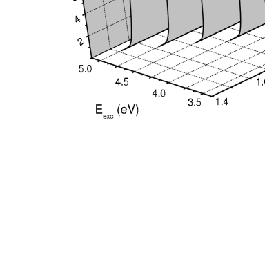
Figure 2: IEDF $S(\epsilon)$ and EDF $f(\epsilon)$ values for zinc oxide given as functions of the excess energy of excited electrons $\epsilon$ and excitation energy $E_{exc}$ .

Figure 3: Dependence of the relaxation rate P on the excess energy $\epsilon$ for zinc oxide. In the inset also the energy dependencies of the total relaxation rate $\Gamma$ and density of states N are given.

Figure 4: Dependence of the EDF setting time $\tau_{s}$ (thick solid line) and energy loss time $\tau_{l}$ (thick dashed line) on the excess energy $\epsilon$ for ZnO. Also the values of the $\tau_{l}$ (thin solid line) and $\tau_{s}$ (thin dashed line) are given calculated with the constant transition probability P= 1 eV/fsec.

It follows from the Fig. 2 that in the case of zinc oxide the main feature of the $S(\omega)$ IEDF function is a gaussian peak whose maximum energy increases linearly with the rise of the excitation energy. This peak corresponds to the vertical transitions from the highest valence band states to the lowest conduction band states for the points located at the $\Gamma-K$ direction of the Brillouine zone and in the vicinity of this direction. With the increase of the excitation energy the wave vector of the transition shifts from the $\Gamma$ to K point. The transition matrix elements of such excitations are much higher than the TME for excitations from all the lower valence band states, so the excitations from the lower states manifest themselves as the low satellites of the main peak. In correspondence with this IEDF function, the quasi-stationary function $f(\omega)$ demonstrates a Fermi-like distribution of the excited electrons in the conduction band, with almost constant number of electrons at the energy levels from the bottom of the conduction band to the energy $E_{exc}-3.4$ eV.

In Figs. 3 and 4 the data concerning electron dynamics in ZnO anatase are given. Fig. 3 also characterizes the applicability of the ”effective phonon” approximation with energy-independent transition probability $P$. The change of the total probability $\Gamma(\epsilon)$ with energy is almost linear beginning from the lowest excess energy $\epsilon=\hbar\omega_{m}$, whereas the density of states $N(\epsilon)$ also changes almost linearly, but reduces to very small values at the low limit. Therefore the value $P(\epsilon)=\Gamma(\epsilon)/N(\epsilon)$ diverges near the bottom of the conduction band, but at the energy above 0.3 eV the change of $P(\epsilon)$ with energy is slow.

The calculated data on the energy loss time $\tau_{l}$ and EDF setting time $\tau_{s}$ are shown in Fig. 4. They demonstrate that the relaxation of the electrons to the bottom of the conduction band occurs within the time less than 500 fsec. The setting of the quasi-stationary electron distribution in presence of the steady in time light source also occurs within the time of no more than 500 fsec. These data are in reasonable correspondence to the experimental data Yama99 ; Sun05 ; Hend07 ; Wen07 . An analysis of the problems of comparing the experimental and theoretical data can be found in the Ref. Zhuk10b .

In Fig. 4 also the data on $\tau_{l}$, $\tau_{s}$ are given calculated with a constant value of the transition probability $P$. In order to obtain the best results the integration interval from 0 to 0.3 eV has been from the calculations excluded. The calculations demonstrate that the approximation of the energy-independent P produces sufficiently good results only at the excess energy more than 0.7 eV. Variation of the $P$-value does not help to improve the correspondence to the results of the calculations with the energy-dependent probability.

In Fig. 5 the density of states and dispersion curves for anatase are given. The conduction band states at the energy from 3.2 to 7.8 eV above the Fermi level are composed mainly of 3d Ti states. The corresponding density of states sharply changes with energy that evokes essential variation of $\Gamma$-probability Zhuk10b . On opposite to the case of ZnO the calculations demonstrate that the band gap of anatase is not direct. The highest valence band state with almost equal energy are observed in $Z$- and $M$-point whereas the lowest conduction band state is in $\Gamma$-point. The decrease of energy of the highest valence states on direction from $M$ to $\Gamma$ points has been confirmed recently on ARPES experiments Emor10 .

Figure 5: Left panel: the density of states of anatase; right panel: energy band structure of anatase near the band gap. Both kinds of data are given with respect to the Fermi level.

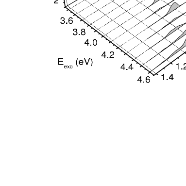
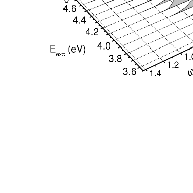
Figure 6: The dependencies of the IEDF $S(\epsilon)$ and EDF $f(\epsilon)$ functions on the excess energy of excited electrons $\epsilon$ and excitation energy $E_{exc}$ for anatase.

At the excitation energy from 3.5 to 3.8 eV the $S(\omega)$ dependencies for anatase also are gaussian peaks accompanied by low-energy satellite. Similarly to the the case of zinc oxide they correspond to the transitions from the highest occupied valence band states to the lowest conduction band states. The wave vectors of these excitations are located on the $\Gamma-Z$ direction or in the vicinity of it. For example, the excitations at 3.5 eV occur from the states near the middle point of the $\Gamma-Z$ direction, the excitations at 3.6 eV occur from the states near $Z$ point, and the excitations at 3.8 eV occur from the states near the $\Gamma$ point. However, contrary to the case of zinc oxide, the TME for excitations from some lower band states are higher than those for the excitations from the highest valence band states. Such are the band states that belong to the 13-th and 14,15-th degenerate dispersion curves on Fig. 4 and the states of general symmetry in the vicinity of these curves. So, when the excitation energy increases up to the value sufficient for the excitations from these lower bands, and this energy is of 3.9 eV, a shift of the $S(\omega)$ peaks to the lower $\omega$ occurs. At energy above this threshold the excitations from the highest valence band states to the lowest conduction band states contribute to only low satellites of the the $S(\omega)$ functions. In comparison with ZnO, this modification of $S(\omega)$ provokes essential change in the corresponding $f(\omega)$ EDF function. At energy above 3.9 eV it is no more a Fermi-like regularity, but is composed of the main peak at $\epsilon$ $\leq$0.6 eV and a low shoulder extending up to the excess energy equal to $E_{exc}-3.2$ eV. So at any $E_{exc}$ and $\epsilon$ the number of excited electrons in anatase is markedly less than in ZnO.

Figure 7: The dependence of the relaxation rate P on the excess energy $\epsilon$ for anatase. In the inset also the energy dependencies of the total relaxation rate $\Gamma$ and density of states are given.

Figure 8: The dependence of the EDF setting time $\tau_{s}$ (thick solid line) and energy loss time $\tau_{l}$ (thick dashed line) on the excess energy $\epsilon$ for anatase. Also the values of the $\tau_{l}$ (thin solid line) and $\tau_{s}$ (thin dashed line) are given calculated with the constant transition probability P= 0.25 eV/fsec.

The characteristics of electron dynamics are given for anatase in Figs. 7 and 8. As in the case of ZnO, the transition probability $P$ has divergence near the bottom of the conduction band. The interval of rapid change of $P$ with energy extends from zero to about 0.7 eV. At higher energy $P$ varies near 0.25 eV/fsec, the value much less than in the case of ZnO. Nevertheless, as it follows from Fig. 8, both the energy-loss time $\tau_{l}$ and EDF setting time $\tau_{s}$ appear to be much less than for ZnO. This is associated with much higher values of density of state that provide higher rate of electron-phonon relaxation. Also the $\tau_{l}$ and $\tau_{s}$ values are shown in Fig. 8 calculated with constant value $P$=0.25 eV and with interval of rapid variations of $P$ excluded from integration. It is evident that these calculations only reproduce the trends of changes, whereas the actual deviations from the exact $\tau_{l},\tau_{s}$-values mounts to 400 %. The variations of the P-value between 0.1 and 0.4 eV/fsec and also of the low limit of integration do not help to improve these results.

V Conclusions

We have proposed a first-principle method for evaluations of the distribution function of the excited electrons in the conduction band of semi-conductors. The approach takes into account the loss of electron energy via electron-phonon coupling, the emergence of new electrons excited by the external light source and redistribution of electrons between the energy levels. The method has been applied to the evaluations of the static electron distribution function in anatase and zinc oxide; the time of energy loss and the time of setting of the static distribution also have been calculated.

The method helps to come also to some conclusions that may have relation to the photocatalytic activity of the compounds. It is generally accepted that the photocatalytic activity of the oxide semiconductors is to a great extent determined by the light absorption because it is proportional to the number of created electron-hole pairs. Therefore the band structure and optical absorption in pure and doped ZnO and TiO₂ was a subject of a great number of calculations, see e.g. Ref. [Cui08, ]. Also a factor important for the photocatalytic activity is the rate of charge transfer between the oxide and molecules absorbed on surface; this rate should be higher than the rate of electron-hole recombination. This factor deserves a special attention, but till now it was only hardly touched in the first-principle approaches. Our calculations permit to discuss one more characteristic of oxides that also can be important. Namely, one should expect that, irrespectively of the details of the processes on the surface, the less is the energy loss of excited electrons in bulk the more is the portion of the absorbed energy of light that can be spent to produce a photochemical reaction. So it is worthwhile to introduce the value

$$e_{ph}(\epsilon)=\hbar\omega_{0}f(\epsilon)\Gamma(\epsilon)$$ (46)

as the measure of the energy transfer to the phonon system. In Fig. 9 we compare these values for ZnO and anatase (the factor $\hbar\omega_{0}$ is omitted). They are given for the excess energy of 0.3 eV, that is the middle energy between the band gap and the edge of the solar light, 4 eV. The $f(\omega)$ value is in this region slightly less for anatase than for ZnO, but the $\Gamma$ value for anatase is much higher. Evidently, this is associated with much higher density of states in the conduction band of anatase. Therefore the rate of energy loss in ZnO appears to be about 5 times less than in anatase.

Figure 9: Left panel: the energy dependencies of the $f(\epsilon)$ and $\Gamma(\epsilon)$ values for ZnO and anatase; right panel: the energy dependencies of the $\Gamma(\epsilon)f(\epsilon)$ products. The data on ZnO are given in solid curves, and the data for anatase are in dash.

This is the factor favoring the higher photocatalytic activity of ZnO. Since this ratio depends on the states of only conduction band and on the electron-phonon coupling of only these states, one can expect that such ratio is valid also for the ZnO and anatase doped with elements producing states inside the band gap. So we may expect that the doped ZnO can probably be more promising material for photocatalytic applications than the doped anatase. The photocatalytic properties of the doped ZnO have been studied much less than those of the doped TiO₂. Nevertheless, there are few papers containing the comparison of activity of ZnO and anatase in the reactions of photo-decolarization of red dye Asl11 ; Kans09 . It has been shown in Asl11 that the ZnO catalyst composed of nano-particles has the activity equal to that of the analogous anatase catalyst, in spite of that the surface area of the anatase catalyst was more extensive. The comparison of the effectiveness of ZnO- and TiO₂-based photo-catalysts in degradation of dyes made by the authors of the Ref. Kans09 demonstrated a 20 - 30 % superiority of the ZnO-based catalysts. There are also examples of the doped ZnO-based catalysts that have high activity in visible light Kana07 ; Shap09 .

References

- (1) O. Carp, C. Huisman, and A. Reller, Progress in Solid State Chemistry 32, 33 (2004).
- (2) H. Lu, H. Li, L. Liao, Y. Tian, M. Shuai, J. C. Li, M. Hu, Q. Fu, and B. Zhu, Nanotechnology 19, 045605 (2008).
- (3) Y. Ni, X. Cao, G. Wu, G. Hu, Z. Yang, and X. Wei, Nanotechnology 18, 155603 (2007).
- (4) O. Girdasova, V. N. Krasilnikov, L. I. Buldakova, M. Iu.Yanchenko, and O. V. Koriakova, Izv. Ross. Akad. Nauk, Ser. Fiz. 73, 1176 (2009).
- (5) M. R. Hoffmann, S. Martin, W. Choi, and D. Bahnemannt, Chem. Rev. 95, 69 (1995).
- (6) S. Kim, W.-D. Kim, K. Kim, C. Hwang, and J. Jeong, Appl. Phys. Lett. 85, 4112 (2004).
- (7) C. Maiti, S. Samanta, G. Dalapati, S. Nandi, and S. Chatterjee, Microelectron. Eng. 72, 253 (2004).
- (8) M. Lane, C. Murray, and F. McFeely, Appl. Phys. Lett. 85, 4112 (2004).
- (9) A. Yamamoto, T. Kido, T. Goto, Y. Chen, T. Yao, and A. Kasuya, Appl. Phys. Lett. 75, 469 (1999).
- (10) E. Hendry, M. Koeberg, and M. Bonn, Phys. Rev. B 76, 045214 (2007).
- (11) X. Wen, J. Davis, D. McDonald, L. Dao, P. Hannaford, V. Coleman, H. Tan, C. Jagadish, K. Koike, S. Sasa, et al., Nanotechnolog 18, 315403 (2007).
- (12) C.-K. Sun, S.-Z. Sun, K.-H. Lin, K. Y.-J. Zhang, H.-L. Liu, S.-C. Liu, and J.-J. Wu, Appl. Phys. Lett. 87, 023106 (2005).
- (13) M. Watanabe, S. Sasaki, and T. Hayashi, J. Lumin. 87 89, 1234 (2000).
- (14) M. Watanabe, T. Hayashi, H. Yagasaki, and S. Sasaki, Int. J. Mod. Phys. B 15, 3997 (2001).
- (15) T. Sekiya, M. Tasaki, K. Wakabayashi, and S. Kurita, Journal of Luminesc. 108, 69 (2004).
- (16) E. Hendry, F. Wang, J. Shan, T. F. Heinz, and M. Bonn, Phys. Rev. B 69, 081101 (2004).
- (17) V. P. Zhukov, E. Chulkov, and P. Echenique, Physical Review B 65, 115116 (2002).
- (18) V. P. Zhukov, E. Chulkov, and P. Echenique, Physical Review Letters 93(9), 096401 (2004).
- (19) R. Knorren, G. Bouzerar, and K. Bennemann, J. Phys.: Condens. Matter 14, R739 (2002).
- (20) S. Baroni, S. de Gironcoli, and A. D. Corso, Rev. of Modern Physics 73, 515 (2001).
- (21) E. Zein, Sov. Phys. Solid State 26, 1825 (1984).
- (22) V. Zhukov, P. Echenique, and E. Chulkov, Phys. Rev. B 82, 094302 (2010).
- (23) V. Zhukov and E. Chulkov, J. Phys.: Condens. Matter 22, 435802 (2010).
- (24) V.G.Tyuterev, S. Obukhov, N. Vast, and J. Sjakste, Phys. Rev. B 84, 035201 (2011).
- (25) S. D. Sarma, J. K. Jain, and R. Jalabert, Physical Review B 37, 6290 (1988).
- (26) S. Komirenko, K. Kim, M. Stroscio, and M. Dutta, J. Phys.: Condens. Matter 13, 6233 (2001).
- (27) D.-J. Jang, G.-T. Lin, C.-L. Wu, C.-L. Hsiao, and L. W. Tu, Appl. Phys. Lett. 91, 092108 (2007).
- (28) Z. Tao, C. S. Ting, and M. Singh, Phys. Rev. Lett. 70, 2467.
- (29) G. Mahan, Many-particle physics (Plenum Press, New York, 1990).
- (30) G. Grimvall, The Electron-Phonon Interactions in Metals (North-Holland, Amsterdam, 1981).
- (31) O. Andersen, O. Jepsen, and M. Sob, in M. Yussouff, ed., Electronic band structure and its applications (Springer, 1987), vol. 283 of Lecture Notes in Physics.
- (32) R. Loudon, The quantum theory of light (Oxford University Press Inc., New York, 1983).
- (33) V. Zainullina, M. Korotin, and V. Zhukov, Physica B 405, 2110 (2010).
- (34) M. Usuda, N. Hamada, T. Kotani, and M. van Schilfgaarde, Phys. Rev. B 66, 125101 (2002).
- (35) M. Emori, M. Sugita, H. Sakama, and K. Ozawa, Photon Factory Activity Report 2009 # 27 Part B p. 98 (2010).
- (36) Y. Cui, H. Du, and L. Wen, J. Mater. Sci. Technol. 24, 675 (2008).
- (37) S. K. Asl, S. K. Sadrnezhaad, M. K. Rad, and D. Ëuner, Turk J. Chem 35, 1 (2011).
- (38) S. K. Kansal, N. Kaur, and S. Singh, Nanoscale Res. Lett. 4, 709 (2009).
- (39) A. Shaporev, Master’s thesis, Institute of General and Inorganic chemistry, Leninski prospect, 31, 119991 Moscow, Russian Federation (2009).
- (40) K. Kanade, B. Kale, J.-O. Baeg, S. M. Lee, C. W. Lee, S.-J. Moon, and H. Chang, Materials Chemistry and Physics 102, 98 (2007).