Asymptotic properties of the sequential empirical ROC, PPV and NPV curves under case-control sampling

Abstract

The receiver operating characteristic (ROC) curve, the positive predictive value (PPV) curve and the negative predictive value (NPV) curve are three measures of performance for a continuous diagnostic biomarker. The ROC, PPV and NPV curves are often estimated empirically to avoid assumptions about the distributional form of the biomarkers. Recently, there has been a push to incorporate group sequential methods into the design of diagnostic biomarker studies. A thorough understanding of the asymptotic properties of the sequential empirical ROC, PPV and NPV curves will provide more flexibility when designing group sequential diagnostic biomarker studies. In this paper, we derive asymptotic theory for the sequential empirical ROC, PPV and NPV curves under case-control sampling using sequential empirical process theory. We show that the sequential empirical ROC, PPV and NPV curves converge to the sum of independent Kiefer processes and show how these results can be used to derive asymptotic results for summaries of the sequential empirical ROC, PPV and NPV curves.

T1Supported by NIH Grants P01-CA53996 and U01-CA86368.

and

1 Introduction

Several recent papers have discussed the application of group sequential methodology to diagnostic biomarker studies [Tang, Emerson and Zhou (2008), Tang and Liu (2010), Pepe et al. (2009)]. Group sequential study designs (i.e., study designs with multiple interim analyses) provide an opportunity to improve the efficiency of diagnostic biomarker studies by allowing studies to terminate early when the candidate marker is clearly superior or inferior to established markers or historical levels of marker performance. Many group sequential methods assume the existence of a test statistic with an independent increments covariance structure [Jennison and Turnbull (2000)]. A thorough understanding of the asymptotic properties of the sequential empirical ROC, PPV and NPV curves and, specifically, verifying that their summary measures have an independent increments covariance structure, would provide great flexibility when designing group sequential diagnostic biomarker studies.

Diagnostic biomarkers are used to classify a patient as a case or a control. A dichotomous biomarker results in either a positive test, indicating that the subject should be classified as a case, or a negative test, indicating that the subject should be classified as a control. Many biomarkers are measured on a continuous scale and a threshold must be defined in order to translate a continuous biomarker into a positive or negative test result. Let $D$ be a Bernoulli random variable indicating disease status with prevalence $\rho$ and let $X$ be a biomarker value with conditional distribution $F(x|D=1)\equiv F_{D}(x)$ and $F(x|D=0)\equiv F_{\bar{D}}(x)$, where $F_{D}(x)$ is the distribution function for the cases and $F_{\bar{D}}(x)$ is the distribution function for the controls. Furthermore, we define $F(x)\equiv F_{D}(x)+(1-\rho)F_{\bar{D}}(x)$ to be the biomarker distribution function for the entire population. Without loss of generality, assume that larger biomarker values are more indicative of disease. For a threshold $c$, a biomarker value $X$ is translated into a positive test result if it is greater than $c$ and a negative test result if it is less than or equal to $c$.

The receiver operating characteristic (ROC) curve summarizes the classification accuracy of a continuous diagnostic biomarker [Pepe (2003)] by reporting the true positive fraction (TPF) and the false positive fraction (FPF) for all possible cut-offs of the marker. For a threshold $c$, $\mathrm{TPF}(c)=P[X>c|D=1]$ and $\mathrm{FPF}(c)=P[X>c|D=0]$. The ROC curve is defined as

$$\mathrm{ROC}(c)=\{(\mathrm{TPF}(c),\mathrm{FPF}(c)),c\in(-\infty,\infty)\}$$

and can alternately be expressed as

$$\mathrm{ROC}(t)=S_{D}(S^{-1}_{\bar{D}}(t)),\qquad t\in(0,1),$$ (1)

where $S_{D}(x)=1-F_{D}(x)$ and $S_{\bar{D}}(x)=1-F_{\bar{D}}(x)$. $\mathrm{ROC}(t)$ can be interpreted as the TPF corresponding to a FPF of $t$. Alternately, one might be interested in the inverse of the ROC curve,

$$\mathrm{ROC}^{-1}(v)=S_{\bar{D}}(S^{-1}_{D}(v)),\qquad v\in(0,1).$$ (2)

$\mathrm{ROC}^{-1}(v)$ is indexed by the TPF and can be interpreted as the FPF corresponding to a TPF of $v$.

The predictive accuracy of a dichotomous biomarker can be summarized by the positive predictive value (PPV) and negative predictive value (NPV). The PPV and NPV curves were proposed as an extension of PPV and NPV to continuous markers [Moskowitz and Pepe (2004), Zheng et al. (2008)]. For a threshold $c$, $\mathrm{PPV}(c)=P[D=1|X>c]$ and $\mathrm{NPV}(c)=P[D=0|X\leq c]$. The PPV and NPV curves are defined as $\mathrm{PPV}(c)$ and $\mathrm{NPV}(c)$ for all $c\in(-\infty,\infty)$. In practice, PPV and NPV curves are indexed by a summary of the marker distribution rather than a generic threshold [Moskowitz and Pepe (2004), Zheng et al. (2008)]. In this paper, we consider the PPV and NPV curves indexed by the FPF and the percentile value in the entire population.

The ROC, PPV and NPV curves are commonly estimated nonparametrically to avoid making assumptions about the form of $F_{D}(x)$ and $F_{\bar{D}}(x)$. This is particularly important in the case of the ROC, PPV and NPV curves because we are often interested in regions of the curve that correspond to the tails of these distributions. For example, a biomarker must possess a high specificity in order to be clinically useful in a low disease risk population screening setting, which corresponds to the upper tail of the biomarker distribution among controls.

Our understanding of the empirical ROC curve is enhanced by knowledge of its asymptotic properties. Hsieh and Turnbull (1996) showed that the empirical ROC curve converges to the sum of two independent Brownian bridges. The asymptotic normality of summary measures of the empirical ROC curve, such as the area under the ROC curve or a point on the ROC curve, can be derived from their work. To our knowledge, no asymptotic theory is available for the empirical PPV and NPV curves.

Tang, Emerson and Zhou (2008) showed that a family of weighted area under the ROC curve (wAUC) statistics has an independent increments covariance structure. It would be beneficial to show that this assumption holds for a larger class of summaries of the ROC curve. In this paper, we develop asymptotic theory for the sequential empirical ROC, PPV and NPV curves. Our results allow us to develop distribution theory for other summaries of the ROC curve and to develop distribution theory for summaries of the PPV and NPV curves.

2 Notation and definitions

Before beginning our discussion of the sequential empirical ROC, PPV and NPV curves, we provide definitions of the sequential empirical estimates for the underlying distribution and quantile functions. Let $X_{D,1},X_{D,2},\ldots,X_{D,n_{D}}$ be i.i.d. marker values for the cases with distribution function, $F_{D}(x)$, and $X_{\bar{D},1},X_{\bar{D},2},\ldots,X_{\bar{D},n_{\bar{D}}}$ be i.i.d. marker values for the controls with distribution function, $F_{\bar{D}}(x)$. Furthermore, let $r_{D}$ and $r_{\bar{D}}$ refer to the proportion of case and controls, respectively, that are observed at a given time point. The sequential empirical estimate of $F_{D}(x)$ is defined as

$$\hat{F}_{D,r_{D}}(x)=\cases{0,&\quad$\displaystyle 0\leq r_{D}<\frac{1}{n_{D}}$,\vspace*{1pt}\cr\displaystyle\frac{1}{[r_{D}n_{D}]}\sum_{i=1}^{[r_{D}n_{D}]}1\{X_{D,i}\leq x\},&\quad$\displaystyle-\infty<x<\infty,\frac{1}{n_{D}}\leq r_{D}\leq 1$,}$$

and the sequential empirical estimate of $F_{D}^{-1}(t)$ is defined as

$$\hat{F}_{D,r_{D}}^{-1}(t)=\cases{X_{D,1,[r_{D}n_{D}]},&\quad if $t=0,0\leq r_{D}\leq 1$,\vspace*{2pt}\cr X_{D,k,[r_{D}n_{D}]},&\quad if $\displaystyle\frac{k-1}{[r_{D}n_{D}]}<t\leq\frac{k}{[r_{D}n_{D}]}$,\vspace*{2pt}\cr&\quad$1\leq k\leq[r_{D}n_{D}],0\leq t\leq 1$,}$$

where $X_{D,1,[r_{D}n_{D}]},X_{D,2,[r_{D}n_{D}]},\ldots,X_{D,[r_{D}n_{D}],[r_{D}n_{D}]}$ are the sequential order statistics of the biomarker values for the cases. The sequential empirical estimates of $S_{D}(x)$ and $S_{D}^{-1}(t)$ are defined as $\hat{S}_{D,r_{D}}(x)=1-\hat{F}_{D,r_{D}}(x)$ and $\hat{S}_{D,r_{D}}^{-1}(t)=\hat{F}_{D,r_{D}}^{-1}(1-t)$. The sequential empirical estimates for the control population are defined in an analogous fashion. The sequential empirical estimates of $F_{D}(x)$ and $F_{\bar{D}}(x)$ lead to a natural definition of the sequential empirical estimates of $F(x)$ and $F^{-1}(t)$,

$$\hat{F}_{r_{D},r_{\bar{D}}}(x)=\rho\hat{F}_{D,r_{D}}(x)+(1-\rho)\hat{F}_{\bar{D},r_{\bar{D}}}(x)$$

and

$$\hat{F}_{r_{D},r_{\bar{D}}}^{-1}(t)=\inf\{x\dvtx\hat{F}_{r_{D},r_{\bar{D}}}(x)\geq t\},$$

where $\rho$ is assumed to be known. $\hat{F}_{r_{D},r_{\bar{D}}}(x)$ is a linear combination of $\hat{F}_{D,r_{D}}(x)$ and $\hat{F}_{\bar{D},r_{\bar{D}}}(x)$ and is therefore indexed by both $r_{D}$, the proportion of cases observed at a given time point, and $r_{\bar{D}}$, the proportion of controls observed at a given time point.

Throughout this paper, we let $0<a<b<1$, $0<c<1$, $0<d<1$ and make the following assumptions: [(A4)]

$F_{D}(x)$ and $F_{\bar{D}}(x)$ are continuous distribution functions with continuous densities $f_{D}(x)$ and $f_{\bar{D}}(x)$, respectively,

$f_{D}(x)>0$ for $x\in(\sup\{x\dvtx F_{D}(x)=0\},\inf\{x\dvtx F_{D}(x)=1\})$,

$f_{\bar{D}}(x)>0$ for $x\in(\sup\{x\dvtx F_{\bar{D}}(x)=0\},\inf\{x\dvtx F_{\bar{D}}(x)=1\})$,

$\frac{n_{D}}{n_{\bar{D}}}\rightarrow\lambda>0$ as $n_{D}\rightarrow\infty$ and $n_{\bar{D}}\rightarrow\infty$, that is, the ratio of cases to controls converges to a constant that is greater than 0. The asymptotic results in Section 3 make use of the Kiefer process. The Kiefer process, $K(t,r)$, is a two-dimensional, mean-zero Gaussian process with covariance

$$\operatorname{Cov}(K(t_{1},r_{1}),K(t_{2},r_{2}))=(t_{1}\wedge t_{2}-t_{1}t_{2})(r_{1}\wedge r_{2}),$$

where $\wedge$ represents the minimum. The Kiefer process behaves like a Brownian bridge in $t$ and Brownian Motion in $r$.

The remainder of this paper proceeds as follows. In Section 3, we develop asymptotic theory for the sequential empirical ROC, PPV and NPV curves. First, we generalize the work of Hsieh and Turnbull (1996) to the sequential empirical ROC curve by showing that the sequential empirical ROC curve converges to the sum of independent Kiefer processes. Next, we develop asymptotic theory for the sequential empirical PPV and NPV curves indexed by the FPF by writing them as functions of the sequential empirical ROC curve. Finally, we follow the approach of Pyke and Shorack (1968) to develop asymptotic theory for the PPV and NPV curves indexed by the percentile value of the marker distribution. We validate our asymptotic results by simulation in Section 4 and illustrate how they can be used to design group sequential diagnostic biomarker studies in Section 5. We conclude with a discussion in Section 6.

3 Asymptotic results

3.1 The sequential empirical ROC curve

In this section, we provide asymptotic results for the sequential empirical ROC curve. Results for the inverse of the sequential empirical ROC curve are nearly identical; we direct the reader to an associated technical report for details [Koopmeiners and Feng (2010)]. The sequential empirical ROC curve, $\widehat{\mathrm{ROC}}_{r_{D},r_{D}}(t)$, is defined by substituting the sequential empirical estimates of $S_{D}(x)$ and $S_{\bar{D}}(x)$ into (1), yielding

$$\widehat{\mathrm{ROC}}_{r_{D},r_{\bar{D}}}(t)=\hat{S}_{D,r_{D}}(\hat{S}^{-1}_{\bar{D},r_{\bar{D}}}(t)),$$

and for ease of notation, we define

$$R_{r_{D},r_{\bar{D}}}(t)\equiv n_{D}^{-1/2}[n_{D}r_{D}]\bigl{(}\widehat{\mathrm{ROC}}_{r_{D},r_{\bar{D}}}(t)-\mathrm{ROC}(t)\bigr{)}.$$

The primary result in this section provides asymptotic theory for $R_{r_{D},r_{\bar{D}}}(t)$. By developing asymptotic theory for $R_{r_{D},r_{\bar{D}}}(t)$, we are also able to develop asymptotic theory for functionals of $R_{r_{D},r_{\bar{D}}}(t)$ as a special case. Theorem 3.1 establishes the convergence of $R_{r_{D},r_{\bar{D}}}(t)$ to the sum of independent Kiefer processes.

Theorem 3.1

Assume (A1)–(A4) hold and let $\frac{f_{D}(S_{\bar{D}}^{-1}(t))}{f_{\bar{D}}(S_{\bar{D}}^{-1}(t))}$ be bounded on $[a,b]$. As $n_{D}\rightarrow\infty$ and $n_{\bar{D}}\rightarrow\infty$

$$R_{r_{D},r_{\bar{D}}}(t)\rightarrow_{d}K_{1}(\mathrm{ROC}(t),r_{D})+\lambda^{1/2}\frac{r_{D}}{r_{\bar{D}}}\biggl{(}\frac{f_{D}(S_{\bar{D}}^{-1}(t))}{f_{\bar{D}}(S_{\bar{D}}^{-1}(t))}\biggr{)}K_{2}(t,r_{\bar{D}})$$

uniformly for $t\in[a,b]$, $r_{D}\in[c,1]$ and $r_{\bar{D}}\in[d,1]$ where $K_{1}$ and $K_{2}$ are independent Kiefer processes.

A proof of Theorem 3.1 can be found in the Appendix. Theorem 3.1 generalizes the results of Hsieh and Turnbull (1996) to the sequential empirical ROC curve. The proof of Theorem 3.1 is similar to the proof found in Hsieh and Turnbull (1996) but our proof relies on the more powerful sequential empirical process theory. Sequential empirical process theory generalizes asymptotic theory for the standard empirical process by introducing a parameter for time. In doing so, asymptotic results for the sequential empirical process involve the Kiefer process. Using properties of the Kiefer process, we are able to easily derive asymptotic results for summaries of the sequential empirical ROC curve and verify that the independent increments assumption holds in many cases. Furthermore, we can recover Hsieh and Turnbull’s result as a special case of Theorem 3.1 by letting $r_{D}$ and $r_{\bar{D}}$ both equal 1.

Corollary 3.2

Assume (A1)–(A4) hold and let $\frac{f_{D}(S_{\bar{D}}^{-1}(t))}{f_{\bar{D}}(S_{\bar{D}}^{-1}(t))}$ be bounded on $[a,b]$. As $n_{D}\rightarrow\infty$ and $n_{\bar{D}}\rightarrow\infty$,

$$R_{1,1}(t)\rightarrow_{d}B_{1}(\mathrm{ROC}(t))+\lambda^{1/2}\biggl{(}\frac{f_{D}(S_{\bar{D}}^{-1}(t))}{f_{\bar{D}}(S_{\bar{D}}^{-1}(t))}\biggr{)}B_{2}(t)$$

uniformly for $t\in[a,b]$ where $B_{1}$ and $B_{2}$ are independent Brownian bridges.

Immediate from Theorem 3.1 and by noting that $K(t,1)=_{d}B(t)$.

An advantage to studying the asymptotic behavior of the sequential empirical ROC curve at the process level, rather than a single point on the sequential empirical ROC curve, is that we are able to study the joint behavior of multiple points on the ROC curve. Corollary 3.3 provides a normal approximation for a vector of points on the sequential empirical ROC curve.

Corollary 3.3

Assume (A1)–(A4) hold and let $\frac{f_{D}(S_{\bar{D}}^{-1}(t))}{f_{\bar{D}}(S_{\bar{D}}^{-1}(t))}$ be bounded on $[a,b]$. For $t_{1},t_{2},\ldots,t_{J}\in(0,1)$, $r_{D,1},r_{D,2},\ldots,r_{D,J}\in(0,1]$ and $r_{\bar{D},1},r_{\bar{D},2},\allowbreak\ldots,r_{\bar{D},J}\in(0,1]$, a vector of arbitrary points on the sequential empirical ROC curve, $(\widehat{\mathrm{ROC}}_{r_{D,1},r_{\bar{D},1}}(t_{1}),\widehat{\mathrm{ROC}}_{r_{D,2},r_{\bar{D},2}}(t_{2}),\ldots,\widehat{\mathrm{ROC}}_{r_{D,J},r_{\bar{D},J}}(t_{J}))$, is approximately multivariate normal with

$$\widehat{\mathrm{ROC}}_{r_{D,j},r_{\bar{D},j}}(t_{j})\sim N\bigl{(}\mathrm{ROC}(t_{j}),\sigma^{2}_{\widehat{\mathrm{ROC}}_{r_{D,j},r_{\bar{D},j}}(t_{j})}\bigr{)},\qquad j=1,2,\ldots,J,$$

where

$$\sigma^{2}_{\widehat{\mathrm{ROC}}_{r_{D,j},r_{\bar{D},j}}(t_{j})}=\frac{\mathrm{ROC}(t_{j})(1-\mathrm{ROC}(t_{j}))}{n_{D}r_{D,j}}+\biggl{(}\frac{f_{D}(S_{\bar{D}}^{-1}(t_{j}))}{f_{\bar{D}}(S_{\bar{D}}^{-1}(t_{j}))}\biggr{)}^{2}\frac{t_{j}(1-t_{j})}{n_{\bar{D}}r_{\bar{D},j}}$$

and

$$\operatorname{Cov}[\widehat{\mathrm{ROC}}_{r_{D,i},r_{\bar{D},i}}(t_{i}),\widehat{\mathrm{ROC}}_{r_{D,j},r_{\bar{D},j}}(t_{j})]$$

$$\qquad=\frac{(r_{D,i}\wedge r_{D,j})(\mathrm{ROC}(t_{i})\wedge\mathrm{ROC}(t_{j})-\mathrm{ROC}(t_{i})\operatorname{ROC}(t_{j}))}{n_{D}r_{D,i}r_{D,j}}$$

$$\qquad\quad{}+\biggl{(}\frac{f_{D}(S_{\bar{D}}^{-1}(t_{i}))}{f_{\bar{D}}(S_{\bar{D}}^{-1}(t_{i}))}\biggr{)}\biggl{(}\frac{f_{D}(S_{\bar{D}}^{-1}(t_{j}))}{f_{\bar{D}}(S_{\bar{D}}^{-1}(t_{j}))}\biggr{)}\frac{(r_{\bar{D},i}\wedge r_{\bar{D},j})(t_{i}\wedge t_{j}-t_{i}t_{j})}{n_{\bar{D}}r_{\bar{D},i}r_{\bar{D},j}}.\vspace*{-3pt}$$

Immediate from Theorem 3.1.

Corollary 3.3 provides the asymptotic covariance for two points at different locations and different times on the sequential empirical ROC curve. This allows us to fully specificy the joint sequential distribution of multiple points on the ROC curve, which allows us to design group sequential diagnostic biomarker studies where multiple points on the ROC curve are treated as multiple endpoints of a group sequential study. For example, we might be interested in $\mathrm{ROC}(t_{1})$ and $\mathrm{ROC}(t_{2})$, where $t_{1}$ is chosen for high specificity to rule patients in for work up and $t_{2}$ is chosen for high sensitivity to rule out patients for invasive work.

Our interest in the sequential empirical ROC curve is motivated by the need to design group sequential diagnostic biomarker studies. Our ability to design group sequential diagnostic biomarker studies would be enhanced by showing that summaries of the sequential empirical ROC curve have an independent increments covariance structure. The simplest summary of the ROC curve is a point on the ROC curve, $\mathrm{ROC}(t)$. $\mathrm{ROC}(t)$ can be interpreted as the sensitivity at a specificity of $1-t$. Corollary 3.4 shows that the sequential empirical estimator of $\mathrm{ROC}(t)$ is asymptotically normal and has independent increments when divided its variance.

Corollary 3.4

Assume (A1)–(A4) hold and let $\frac{f_{D}(S_{\bar{D}}^{-1}(t))}{f_{\bar{D}}(S_{\bar{D}}^{-1}(t))}$ be bounded on $[a,b]$. For $t\in(0,1)$ and J stopping times, $(\widehat{\mathrm{ROC}}_{r_{D,1},r_{\bar{D},1}}(t),\widehat{\mathrm{ROC}}_{r_{D,2},r_{\bar{D},2}}(t),\allowbreak\ldots,\widehat{\mathrm{ROC}}_{r_{D,J},r_{\bar{D},J}}(t))$, is approximately multivariate normal with

$$\widehat{\mathrm{ROC}}_{r_{D,i},r_{\bar{D},i}}(t)\sim N\bigl{(}\mathrm{ROC}(t),\sigma^{2}_{\widehat{\mathrm{ROC}}_{r_{D,i},r_{\bar{D},i}}(t)}\bigr{)},\qquad i=1,2,\ldots,J,\vspace*{-2pt}$$

and

$$\operatorname{Cov}[\widehat{\mathrm{ROC}}_{r_{D,i},r_{\bar{D},i}}(t),\widehat{\mathrm{ROC}}_{r_{D,j},r_{\bar{D},j}}(t)]$$

$$\qquad=\operatorname{Var}[\widehat{\mathrm{ROC}}_{r_{D,j},r_{\bar{D},j}}(t)]=\sigma^{2}_{\widehat{\mathrm{ROC}}_{r_{D,j},r_{\bar{D},j}}(t)},\qquad r_{i}\leq r_{j},\vspace*{-2pt}$$

where $\sigma^{2}_{\widehat{\mathrm{ROC}}_{r_{D,j},r_{\bar{D},j}}(t)}$ is defined as in Corollary 3.3.

Immediate from Corollary 3.3.

Asymptotic theory for other summary measures of the ROC curve, such as the area under the curve or the partial area under the curve, can also be derived from Theorem 3.1. This illustrates the flexibility of Theorem 3.1. By developing distribution theory for the sequential empirical ROC curve, we are able to derive distribution theory for summaries of the ROC curve as a special case.

3.2 The sequential empirical PPV and NPV curves indexed by the false positive fraction

In this section, we consider the sequential empirical PPV and NPV curves indexed by the false positive fraction, $t$. The PPV and NPV curve indexed by the false positive fraction can be written as a function of the ROC curve and their asymptotic properties can be derived using the results from Section 3.1. Asymptotic results for the PPV and NPV curve indexed by the true positive fraction, $v$, can similarly be derived by writing the PPV and NPV curve as a function of the inverse of the ROC curve but are not presented in this paper. The interested reader is directed to Koopmeiners and Feng (2010) for details.

The PPV and NPV curves indexed by the false positive fraction are defined as $\mathrm{PPV}(t)=P[D=1|X>S_{\bar{D}}^{-1}(t)]$ and $\mathrm{NPV}(t)=P[D=0|X\leq S_{\bar{D}}^{-1}(t)]$ for all $t\in(0,1)$ and can be written as functions of the ROC curve as follows:

$$\mathrm{PPV}(t)=\frac{\mathrm{ROC}(t)\rho}{\mathrm{ROC}(t)\rho+t(1-\rho)}$$ (3)

and

$$\mathrm{NPV}(t)=\frac{(1-t)(1-\rho)}{(1-\mathrm{ROC}(t))\rho+(1-t)(1-\rho)}.$$ (4)

The sequential empirical estimators of $\mathrm{PPV}(t)$ and $\mathrm{NPV}(t)$ are defined be plugging the sequential empirical estimator of $\mathrm{ROC}(t)$ into (3) and (4), yielding

$$\widehat{\mathrm{PPV}}_{r_{D},r_{\bar{D}}}(t)=\frac{\widehat{\mathrm{ROC}}_{r_{D},r_{\bar{D}}}(t)\rho}{\widehat{\mathrm{ROC}}_{r_{D},r_{\bar{D}}}(t)\rho+t(1-\rho)}$$

and

$$\widehat{\mathrm{NPV}}_{r_{D},r_{\bar{D}}}(t)=\frac{(1-t)(1-\rho)}{(1-\widehat{\mathrm{ROC}}_{r_{D},r_{\bar{D}}}(t))\rho+(1-t)(1-\rho)}.$$

From this point forward, we only consider $\widehat{\mathrm{PPV}}_{r_{D},r_{\bar{D}}}(t)$ and note that results for $\widehat{\mathrm{NPV}}_{r_{D},r_{\bar{D}}}(t)$ are nearly identical. Again, for ease of notation, we define

$$P_{r_{D},r_{\bar{D}}}(t)\equiv n_{D}^{-1/2}[n_{D}r_{D}]\bigl{(}\widehat{\mathrm{PPV}}_{r_{D},r_{\bar{D}}}(t)-\mathrm{PPV}(t)\bigr{)}.$$

We begin by using the results of Section 3.1 to derive asymptotic theory for $P_{r_{D},r_{\bar{D}}}(t)$. Theorem 3.5 establishes the convergence of $P_{r_{D},r_{\bar{D}}}(t)$ to the sum of two independent Kiefer processes.

Theorem 3.5

Assume (A1)–(A4) hold and let $\frac{f_{D}(S_{\bar{D}}^{-1}(t))}{f_{\bar{D}}(S_{\bar{D}}^{-1}(t))}$ be bounded on $[a,b]$. As $n_{D}\rightarrow\infty$ and $n_{\bar{D}}\rightarrow\infty$

$$P_{r_{D},r_{\bar{D}}}(t) \rightarrow_{d} \biggl{(}\frac{t(1-\rho)\rho}{(\mathrm{ROC}(t)\rho+t(1-\rho))^{2}}\biggr{)}$$

$${}\times\biggl{(}K_{1}(\mathrm{ROC}(t),r_{D})+\lambda^{1/2}\frac{r_{D}}{r_{\bar{D}}}\biggl{(}\frac{f_{D}(S_{\bar{D}}^{-1}(t))}{f_{\bar{D}}(S_{\bar{D}}^{-1}(t))}\biggr{)}K_{2}(t,r_{\bar{D}})\biggr{)}$$

uniformly for $t\in[a,b]$, $r_{D}\in[c,1]$ and $r_{\bar{D}}\in[d,1]$ where $K_{1}$ and $K_{2}$ are independent Kiefer processes.

The proof of Theorem 3.5 relies on writing $P_{r_{D},r_{\bar{D}}}(t)$ as a functionof $R_{r_{D},r_{\bar{D}}}(t)$

$$P_{r_{D},r_{\bar{D}}}(t) = \biggl{(}\frac{\widehat{\mathrm{ROC}}_{r_{D},r_{\bar{D}}}(t)\rho}{\widehat{\mathrm{ROC}}_{r_{D},r_{\bar{D}}}(t)\rho+t(1-\rho)}-\frac{\mathrm{ROC}(t)\rho}{\mathrm{ROC}(t)\rho+t(1-\rho)}\biggr{)}$$

$${}\times\bigl{(}{\widehat{\mathrm{ROC}}_{r_{D},r_{\bar{D}}}(t)-\mathrm{ROC}(t)}\bigr{)}^{-1}R_{r_{D},r_{\bar{D}}}(t)$$

and applying the results of Theorem 3.1. The first term converges to

$$\biggl{(}\frac{t(1-\rho)\rho}{(\mathrm{ROC}(t)\rho+t(1-\rho))^{2}}\biggr{)}$$

and $R_{r_{D},r_{\bar{D}}}(t)$ converges to the sum of two independent Kiefer process by Theorem 3.1. A formal proof of Theorem 3.5 can be found in Koopmeiners and Feng (2010).

From Theorem 3.5, we can prove analogous results to Corollaries 3.3 and 3.4 for the sequential empirical PPV curve indexed by the FPF. Namely, that an arbitrary vector of points on the sequential empirical PPV curve follows a multivariate normal distribution and the sequential empirical estimate of a point on the PPV curve is approximately normally distributed with an independent increments covariance structure. We leave the formal statement of these corollaries for the Appendix but present the form of the covariance between two arbitrary points on the sequential empirical PPV curve:

$$\operatorname{Cov}[\widehat{\mathrm{PPV}}_{r_{D,i},r_{\bar{D},i}}(t_{i}),\widehat{\mathrm{PPV}}_{r_{D,j},r_{\bar{D},j}}(t_{j})]$$

$$\qquad=\biggl{(}\frac{t_{i}(1-\rho)\rho}{(\mathrm{ROC}(t_{i})\rho+t_{i}(1-\rho))^{2}}\biggr{)}\biggl{(}\frac{t_{j}(1-\rho)\rho}{(\mathrm{ROC}(t_{j})\rho+t_{j}(1-\rho))^{2}}\biggr{)}$$

$$\qquad\quad{}\times\operatorname{Cov}[\widehat{\mathrm{ROC}}_{r_{D,i},r_{\bar{D},i}}(t_{i}),\widehat{\mathrm{ROC}}_{r_{D,j},r_{\bar{D},j}}(t_{j})].$$

$\mathrm{PPV}(t)$ is a function of $\mathrm{ROC}(t)$ and, therefore, distribution theory for a vector of points on the PPV curve can also be derived using the delta method and Corollary 3.3.

Asymptotic theory for the fixed-sample empirical PPV curve indexed by the FPF, which was previously unavailable, can be derived as a special case of Theorem 3.5 by letting $r_{D}$ and $r_{\bar{D}}$ equal 1. The fixed-sample empirical PPV curve converges to the sum of independent Brownian bridges

$$P_{1,1}(t) \rightarrow_{d} \biggl{(}\frac{t(1-\rho)\rho}{(\mathrm{ROC}(t)\rho+t(1-\rho))^{2}}\biggr{)}$$

$${}\times\biggl{(}B_{1}(\mathrm{ROC}(t))+\lambda^{1/2}\biggl{(}\frac{f_{D}(S_{\bar{D}}^{-1}(t))}{f_{\bar{D}}(S_{\bar{D}}^{-1}(t))}\biggr{)}B_{2}(t)\biggr{)},$$

which allows us to derive a normal approximation for the empirical estimate of a point on the PPV curve

$$\widehat{\mathrm{PPV}}_{1,1}(t)\sim N\biggl{(}\mathrm{PPV}(t),\biggl{(}\frac{t(1-\rho)\rho}{(\mathrm{ROC}(t)\rho+t(1-\rho))^{2}}\biggr{)}^{2}\sigma^{2}_{\widehat{\mathrm{ROC}}_{1,1}(t)}\biggr{)},$$

where $\sigma^{2}_{\widehat{\mathrm{ROC}}_{1,1}(t)}$ is defined as in Corollary 3.3.

3.3 The sequential empirical PPV and NPV curves indexed by the percentile value

Finally, we consider the PPV and NPV curves indexed by the proportion of the population that are classified as negative, $u$, and positive, $1-u$. In this case, the PPV and NPV curves are defined as $\mathrm{PPV}(u)=P[D=1|X>F^{-1}(u)]$ and $\mathrm{NPV}(u)=P[D=0|X\leq F^{-1}(u)]$ for all $u\in(0,1)$. Under this indexing, the PPV curve can be written as

$$\mathrm{PPV}(u)=\frac{S_{D}(F^{-1}(u))\rho}{1-u},$$ (5)

and since the NPV curve can be written as

$$\mathrm{NPV}(u)=\frac{u-\rho}{u}+\frac{1-u}{u}\operatorname{PPV}(u),$$ (6)

it suffices to study the PPV curve when considering estimation of the NPV curve.

The sequential empirical estimator of $\mathrm{PPV}(u)$ is found by substituting the sequential empirical estimators of $S_{D}(x)$ and $F(x)$, along with the known value of $\rho$, into (5),

$$\widehat{\mathrm{PPV}}_{r_{D},r_{\bar{D}}}(u)=\frac{\hat{S}_{D,r_{D}}(\hat{F}_{r_{D},r_{\bar{D}}}^{-1}(u))\rho}{1-u},$$ (7)

and the sequential empirical estimator of $\mathrm{NPV}(u)$ is found by substituting the sequential empirical estimator of $\mathrm{PPV}(u)$ into (6),

$$\widehat{\mathrm{NPV}}_{r_{D},r_{\bar{D}}}(u)=\frac{u-\rho}{u}+\frac{1-u}{u}\,\widehat{\mathrm{PPV}}_{r_{D},r_{\bar{D}}}(u).$$ (8)

Finally, we define,

$$P_{r_{D},r_{\bar{D}}}(u)=n_{D}^{-1/2}[n_{D}r_{D}]\bigl{(}\widehat{\mathrm{PPV}}_{r_{D},r_{\bar{D}}}(u)-\mathrm{PPV}(u)\bigr{)}$$

and

$$N_{r_{D},r_{\bar{D}}}(u)=n_{D}^{-1/2}[n_{D}r_{D}]\bigl{(}\widehat{\mathrm{NPV}}_{r_{D},r_{\bar{D}}}(u)-\mathrm{NPV}(u)\bigr{)}$$

for mathematical convenience. We begin by developing distribution theory for $P_{r_{D},r_{\bar{D}}}(u)$. Theorem 3.6 establishes the convergence of the sequential empirical PPV curve to the sum of two independent Kiefer processes.

Theorem 3.6

Assume (A1)–(A4) hold and let $\frac{f_{D}(F^{-1}(u))}{f(F^{-1}(u))}$ be bounded on $[a,b]$. As $n_{D}\rightarrow\infty$ and $n_{\bar{D}}\rightarrow\infty$

$$P_{r_{D},r_{\bar{D}}}(u) \rightarrow_{d} -\frac{\rho(1-\rho)}{1-u}\frac{f_{\bar{D}}(F^{-1}(u))}{f(F^{-1}(u))}K_{1}(F_{D}(F^{-1}(u)),r_{D})$$

$${}+\frac{\rho(1-\rho)}{1-u}\frac{f_{D}(F^{-1}(u))}{f(F^{-1}(u))}\sqrt{\lambda}\frac{r_{D}}{r_{\bar{D}}}K_{2}(F_{\bar{D}}(F^{-1}(u)),r_{\bar{D}})$$

uniformly for $u\in[a,b]$, $r_{D}\in[c,1]$ and $r_{\bar{D}}\in[d,1]$ where $K_{1}$ and $K_{2}$ are independent Kiefer processes.

The proof of Theorem 3.6 is complicated by the fact that $\hat{S}_{D,r_{D}}(x)$and $\hat{F}_{r_{D},r_{\bar{D}}}^{-1}(t)$ are correlated because $\hat{F}_{r_{D},r_{\bar{D}}}(x)$ is a linear combinationof $\hat{F}_{D,r_{D}}(x)$ and $\hat{F}_{\bar{D},r_{\bar{D}}}(x)$. In contrast, the sequential empirical ROC curve and the sequential empirical PPV curve indexed by the FPF are functionals of two independent sequential empirical estimators, $\hat{S}_{D,r_{D}}(x)$ and $\hat{S}_{\bar{D},r_{\bar{D}}}^{-1}(t)$, which makes it easier to show that $R_{r_{D},r_{\bar{D}}}(t)$ and $P_{r_{D},r_{\bar{D}}}(t)$ converge to the sum of independent Kiefer processes. To account for the correlation between $\hat{S}_{D,r_{D}}(x)$ and $\hat{F}_{r_{D},r_{\bar{D}}}^{-1}(t)$, we follow the approach of Pyke and Shorack (1968), who prove a similar result for two correlated, fixed-sample empirical processes. The proof of Theorem 3.6 can be found in the Appendix.

Theorem 3.6 also establishes asymptotic theory for the sequential empirical NPV curve because $\widehat{\mathrm{NPV}}_{r_{D},r_{\bar{D}}}(t)$ is a function of $\widehat{\mathrm{PPV}}_{r_{D},r_{\bar{D}}}(t)$. Corollary 3.7 establishes the convergence of $N_{r_{D},r_{\bar{D}}}(t)$ to the sum of two independent Kiefer processes.

Corollary 3.7

Assume (A1)–(A4) hold and let $\frac{f_{D}(F^{-1}(u))}{f(F^{-1}(u))}$ be bounded on $[a,b]$. As $n_{D}\rightarrow\infty$ and $n_{\bar{D}}\rightarrow\infty$

$$N_{r_{D},r_{\bar{D}}}(u) \rightarrow_{d} -\frac{\rho(1-\rho)}{u}\frac{f_{\bar{D}}(F^{-1}(u))}{f(F^{-1}(u))}K_{1}(F_{D}(F^{-1}(u)),r_{D})$$

$${}+\frac{\rho(1-\rho)}{u}\frac{f_{D}(F^{-1}(u))}{f(F^{-1}(u))}\sqrt{\lambda}\frac{r_{D}}{r_{\bar{D}}}K_{2}(F_{\bar{D}}(F^{-1}(u)),r_{\bar{D}})$$

uniformly for $u\in[a,b]$, $r_{D}\in[c,1]$ and $r_{\bar{D}}\in[d,1]$ where $K_{1}$ and $K_{2}$ are independent Kiefer processes.

Corollary 3.7 is immediate from Theorem 3.6 by noting that

$$N_{r_{D},r_{\bar{D}}}(t)=\frac{1-u}{u}P_{r_{D},r_{\bar{D}}}(t).$$

As with the ROC curve and the PPV curve indexed by the FPF, Theorem 3.6 and Corollary 3.7 allow us to develop distribution theory for summaries of the PPV and NPV curve indexed by u. Distribution theory for a vector of points on the PPV or NPV curve is left for the Appendix but we choose to highlight the joint distribution of the sequential empirical estimate of a single point on the PPV or NPV curve. Corollary 3.8 establishes that the sequential empirical estimate of a point on the PPV or NPV curve is asymptotically normal and has independent increments when divided by its variance.

Corollary 3.8

Assume (A1)–(A4) hold and let $\frac{f_{D}(F^{-1}(u))}{f(F^{-1}(u))}$ be bounded on $[a,b]$. For $u\in(0,1)$ and J stopping times: [(A)]

$(\widehat{\mathrm{PPV}}_{r_{D,1},r_{\bar{D},1}}(u),\widehat{\mathrm{PPV}}_{r_{D,2},r_{\bar{D},2}}(u),\ldots,\widehat{\mathrm{PPV}}_{r_{D,J},r_{\bar{D},J}}(u))$, is approximately multivariate normal with

$$\widehat{\mathrm{PPV}}_{r_{D,i},r_{\bar{D},i}}(u)\sim N\bigl{(}\mathrm{PPV}(u),\sigma^{2}_{\widehat{\mathrm{PPV}}_{r_{D,i},r_{\bar{D},i}}(u)}\bigr{)},\qquad i=1,2,\ldots,J,$$

and

$$\operatorname{Cov}[\widehat{\mathrm{PPV}}_{r_{D,i},r_{\bar{D},i}}(u),\widehat{\mathrm{PPV}}_{r_{D,j},r_{\bar{D},j}}(u)]$$

$$\qquad=\operatorname{Var}[\widehat{\mathrm{PPV}}_{r_{D,j},r_{\bar{D},j}}(u)]=\sigma^{2}_{\widehat{\mathrm{PPV}}_{r_{D,j},r_{\bar{D},j}}(u)},\qquad r_{i}\leq r_{j},$$

where

$$\sigma^{2}_{\widehat{\mathrm{PPV}}_{r_{D,j},r_{\bar{D},j}}(u)} = \biggl{(}\frac{f_{\bar{D}}(F^{-1}(u))}{f(F^{-1}(u))}(1-\rho)\biggr{)}^{2}\operatorname{PPV}(u)\biggl{(}\frac{\rho}{1-u}-\mathrm{PPV}(u)\biggr{)}$$

$${}\times\frac{1}{n_{D}r_{D,j}}$$

$${}+\biggl{(}\frac{f_{D}(F^{-1}(u))}{f(F^{-1}(u))}\rho\biggr{)}^{2}\bigl{(}1-\mathrm{PPV}(u)\bigr{)}\biggl{(}\frac{u-\rho}{1-u}+\mathrm{PPV}(u)\biggr{)}$$

$$\hskip 11.0pt{}\times\frac{1}{n_{\bar{D}}r_{\bar{D},j}}.$$

$(\widehat{\mathrm{NPV}}_{r_{D,1},r_{\bar{D},1}}(u),\widehat{\mathrm{NPV}}_{r_{D,2},r_{\bar{D},2}}(u),\ldots,\widehat{\mathrm{NPV}}_{r_{D,J},r_{\bar{D},J}}(u))$, is approximately multivariate normal with,

$$\widehat{\mathrm{NPV}}_{r_{D,i},r_{\bar{D},i}}(u)\sim N\bigl{(}\mathrm{NPV}(u),\sigma^{2}_{\widehat{\mathrm{NPV}}_{r_{D,i},r_{\bar{D},i}}(u)}\bigr{)},\qquad i=1,2,\ldots,J,$$

and

$$\operatorname{Cov}[\widehat{\mathrm{NPV}}_{r_{D,i},r_{\bar{D},i}}(u),\widehat{\mathrm{NPV}}_{r_{D,j},r_{\bar{D},j}}(u)]$$

$$\qquad=\operatorname{Var}[\widehat{\mathrm{NPV}}_{r_{D,j},r_{\bar{D},j}}(u)]=\sigma^{2}_{\widehat{\mathrm{NPV}}_{r_{D,j},r_{\bar{D},j}}(u)},\qquad r_{i}\leq r_{j},$$

where

$$\sigma^{2}_{\widehat{\mathrm{NPV}}_{r_{D,j},r_{\bar{D},j}}(u)} = \biggl{(}\frac{f_{\bar{D}}(F^{-1}(u))}{f(F^{-1}(u))}(1-\rho)\biggr{)}^{2}\biggl{(}\mathrm{NPV}(u)+\frac{\rho-u}{u}\biggr{)}\bigl{(}1-\mathrm{NPV}(u)\bigr{)}$$

$${}\times\frac{1}{n_{D}r_{D,j}}$$

$${}+\biggl{(}\frac{f_{D}(F^{-1}(u))}{f(F^{-1}(u))}\rho\biggr{)}^{2}\operatorname{NPV}(u)\biggl{(}\frac{1-\rho}{u}-\mathrm{NPV}(u)\biggr{)}$$

$$\hskip 11.0pt{}\times\frac{1}{n_{\bar{D}}r_{\bar{D},j}}.$$

It is immediate from Theorem 3.6 and Corollary 3.7 that $\widehat{\mathrm{PPV}}_{r_{D},r_{\bar{D}}}(u)$ and $\widehat{\mathrm{NPV}}_{r_{D},r_{\bar{D}}}(u)$ are asymptotically normal with an independent increments covariance structure. By noting that

$$F_{D}(F^{-1}(u))=1-\frac{1-u}{\rho}\operatorname{PPV}(u)=\frac{u}{\rho}\bigl{(}1-\mathrm{NPV}(u)\bigr{)}$$

and

$$F_{\bar{D}}(F^{-1}(u))=1-\frac{1-u}{1-\rho}\bigl{(}1-\mathrm{PPV}(u)\bigr{)}=\frac{u}{1-\rho}\operatorname{NPV}(u),$$

we can write the asymptotic variances of $\widehat{\mathrm{PPV}}_{r_{D},r_{\bar{D}}}(u)$ and $\widehat{\mathrm{NPV}}_{r_{D},r_{\bar{D}}}(u)$ as functions of $\mathrm{PPV}(u)$ and $\mathrm{NPV}(u)$, respectively. This provides a better understanding of the mean-variance relationship for the asymptotic distributions of $\widehat{\mathrm{PPV}}_{r_{D},r_{\bar{D}}}(u)$ and $\widehat{\mathrm{NPV}}_{r_{D},r_{\bar{D}}}(u)$ and, perhaps, provides a form of the variance that is easier to work with in practical situations (i.e., study design, estimating the standard error, etc.).

An important component of Theorem 3.6 and Corollary 3.7 is that not only do $P_{r_{D},r_{\bar{D}}}(u)$ and $N_{r_{D},r_{\bar{D}}}(u)$ converge to the sum of independent Kiefer processes, but they both converge to the same two Kiefer processes. As a result, we are able to derive the correlation between a point on the PPV curve and a point on the NPV curve. Corollary 3.9 provides a bivariate normal approximation for a point on the PPV and a point on the NPV curve.

Corollary 3.9

Assume (A1)–(A4) hold and let $\frac{f_{D}(F^{-1}(u))}{f(F^{-1}(u))}$ be bounded on $[a,b]$. For $u_{1},u_{2}\in(0,1)$, $(\widehat{\mathrm{PPV}}_{r_{D,1},r_{\bar{D},1}}(u_{1}),\widehat{\mathrm{NPV}}_{r_{D,2},r_{\bar{D},2}}(u_{2}))$, is approximately bivariate normally distributed with

$$\widehat{\mathrm{PPV}}_{r_{D,1},r_{\bar{D},1}}(u_{1})\sim N\bigl{(}\mathrm{PPV}(u),\sigma^{2}_{\widehat{\mathrm{PPV}}_{r_{D,1},r_{\bar{D},1}}(u_{1})}\bigr{)}$$

and

$$\widehat{\mathrm{NPV}}_{r_{D,2},r_{\bar{D},2}}(u_{2})\sim N\bigl{(}\mathrm{NPV}(u),\sigma^{2}_{\widehat{\mathrm{NPV}}_{r_{D,2},r_{\bar{D},2}}(u_{2})}\bigr{)}$$

with

$$\operatorname{Cov}[\widehat{\mathrm{PPV}}_{r_{D,1},r_{\bar{D},1}}(u_{1}),\widehat{\mathrm{NPV}}_{r_{D,2},r_{\bar{D},2}}(u_{2})]$$

$$\qquad=\frac{(1-\rho)^{2}u_{1}(1-u_{2})}{(1-u_{1})u_{2}}\frac{f_{\bar{D}}(F^{-1}(u_{1}))}{f(F^{-1}(u_{1}))}\frac{f_{\bar{D}}(F^{-1}(u_{2}))}{f(F^{-1}(u_{2}))}$$

$$\qquad\quad{}\times\frac{(r_{D,1}\wedge r_{D,2})(1-\mathrm{NPV}(u_{1}))\operatorname{PPV}(u_{2})}{n_{D}r_{D,1}r_{D,2}}$$

$$\qquad\quad{}+\frac{\rho^{2}u_{1}(1-u_{2})}{(1-u_{1})u_{2}}\frac{f_{D}(F^{-1}(u_{1}))}{f(F^{-1}(u_{1}))}\frac{f_{D}(F^{-1}(u_{2}))}{f(F^{-1}(u_{2}))}$$

$$\qquad\quad\hskip 11.0pt{}\times\frac{(r_{\bar{D},2}\wedge r_{\bar{D},2})\operatorname{NPV}(u_{1})(1-\mathrm{PPV}(u_{2}))}{n_{D}r_{D,1}r_{D,2}},$$

when $u_{1}\leq u_{2}$ and

$$\operatorname{Cov}[\widehat{\mathrm{PPV}}_{r_{D,1},r_{\bar{D},1}}(u_{1}),\widehat{\mathrm{NPV}}_{r_{D,2},r_{\bar{D},2}}(u_{2})]$$

$$\qquad=(1-\rho)^{2}\frac{f_{\bar{D}}(F^{-1}(u_{1}))}{f(F^{-1}(u_{1}))}\frac{f_{\bar{D}}(F^{-1}(u_{2}))}{f(F^{-1}(u_{2}))}$$

$$\qquad\quad{}\times\frac{(r_{D,1}\wedge r_{D,2})(1-\mathrm{NPV}(u_{2}))\operatorname{PPV}(u_{1})}{n_{D}r_{D,1}r_{D,2}}$$

$$\qquad\quad{}+\rho^{2}\frac{f_{D}(F^{-1}(u_{1}))}{f(F^{-1}(u_{1}))}\frac{f_{D}(F^{-1}(u_{2}))}{f(F^{-1}(u_{2}))}$$

$$\qquad\quad\hskip 11.0pt{}\times\frac{(r_{\bar{D},2}\wedge r_{\bar{D},2})\operatorname{NPV}(u_{2})(1-\mathrm{PPV}(u_{1}))}{n_{D}r_{D,1}r_{D,2}},$$

when $u_{2}\leq u_{1}$, where $\sigma^{2}_{\widehat{\mathrm{PPV}}_{r_{D,1},r_{\bar{D},1}}(u_{1})}$ and $\sigma^{2}_{\widehat{\mathrm{NPV}}_{r_{D,2},r_{\bar{D},2}}(u_{2})}$ are defined as in Corollary 3.8.

The case of a point on the PPV curve and a point on the NPV curve is presented for simplicity but Corollary 3.9 can be extended to an arbitrary vector of points on the PPV and NPV curves. Corollary 3.9 has obvious practical implications. It is not uncommon to classify the bottom $u_{1}\times 100$% of the population as “low-risk,” the top $(1-u_{2})\times 100$% of the population as “high-risk” and the remainder of the population as “moderate-risk.” In this case, one would be interested in the NPV of the low-risk group and the PPV of the high-risk group. Corollary 3.9 provides the joint convergence of these two estimates.

Finally, we note that asymptotic results for the fixed-sample empirical PPV and NPV curves indexed by the percentile value of the marker distribution can be derived as a special case of the results in this section. It is immediate from Theorem 3.6 and Corollary 3.7 that the fixed-sample empirical PPV and NPV curves converge to the sum of independent Brownian bridges by letting $r_{D}$ and $r_{\bar{D}}$ both equal 1. Furthermore, Corollary 3.8 provides a normal approximation for the fixed-sample empirical estimate of a point on the PPV or NPV curve for the special case when $J=1$.

4 Finite sample properties

A simulation study was completed to assess the finite sample properties of the results in Theorems 3.1, 3.5 and 3.6. We simulated 10,000 studies with $n_{\bar{D}}$ controls and $n_{D}$ cases. Biomarker values for the controls were drawn from a standard normal distribution and biomarker values for the cases were drawn from a normal distribution with mean and standard deviation equal to 1. A prevalence of 0.2 was used for estimation of the PPV curve. Figure 1 presents the true ROC and PPV curves for this scenario. For each realization, we calculated

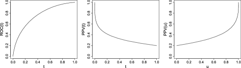
Figure 1: True ROC and PPV curves for the scenario considered in Section 4.

$R_{r_{D},r_{\bar{D}}}(t)$, $P_{r_{D},r_{\bar{D}}}(t)$ and $P_{r_{D},r_{\bar{D}}}(u)$ and evaluated the expected value, normality and covariance for various combinations of $r_{D}$, $r_{\bar{D}}$ and $t$ or $u$. Normality was evaluated by providing a summary of information found in a normal q-q plot. Instead of providing the entire plot, we provide the (simulated) probability of being less than the 5th, 25th, 50th, 75th and 95th percentile of a normal distribution with variance derived using the results in Theorems 3.1, 3.5 and 3.6. Similarly, the simulated covariance matrices were compared to the theoretical covariance matrices derived using the results in Theorems 3.1, 3.5 and 3.6.

== 5th 25th 50th 75th 95th Observed Theoretical Mean %tile %tile %tile %tile %tile covariance matrix covariance matrix $n_{D}=50$, $n_{\bar{D}}=50$ $R_{0.4,0.7}(0.4)$ 0.01 0.05 $0.17$ $0.46$ $0.63$ 0.98 $0.1$ $0.117$ $0.079$ $0.103$ 0.104 0.129 $0.081$ $0.104$ $R_{1,1}(0.4)$ 0.02 0.07 $0.2$ $0.44$ $0.74$ 0.97 $0.318$ $0.104$ $0.262$ 0.322 $0.104$ $0.26$ $R_{0.4,0.7}(0.2)$ 0.03 0.04 $0.22$ $0.47$ $0.73$ 0.96 $0.161$ $0.201$ $0.171$ $0.225$ $R_{1,1}(0.2)$ 0.05 0.04 $0.2$ $0.47$ $0.68$ 0.93 $0.544$ $0.563$ $n_{D}=100$, $n_{\bar{D}}=100$ $R_{0.4,0.7}(0.4)$ 0.01 0.05 $0.21$ $0.41$ $0.78$ 0.97 $0.101$ $0.12$ $0.08$ $0.102$ 0.104 0.129 $0.081$ $0.104$ $R_{1,1}(0.4)$ 0.02 0.05 $0.24$ $0.48$ $0.76$ 0.96 $0.318$ $0.104$ $0.26$ 0.322 $0.104$ $0.26$ $R_{0.4,0.7}(0.2)$ 0.03 0.04 $0.2$ $0.45$ $0.73$ 0.95 $0.164$ $0.205$ $0.171$ $0.225$ $R_{1,1}(0.2)$ 0.05 0.04 $0.23$ $0.47$ $0.73$ 0.95 $0.55$ $0.563$ $n_{D}=200$, $n_{\bar{D}}=200$ $R_{0.4,0.7}(0.4)$ 0.01 0.06 $0.22$ $0.44$ $0.7$ 0.96 $0.104$ $0.121$ $0.081$ $0.102$ 0.104 0.129 $0.081$ $0.104$ $R_{1,1}(0.4)$ 0.02 0.05 $0.25$ $0.48$ $0.72$ 0.95 $0.317$ $0.104$ $0.259$ 0.322 $0.104$ $0.26$ $R_{0.4,0.7}(0.2)$ 0.03 0.04 $0.25$ $0.5$ $0.7$ 0.94 $0.168$ $0.212$ $0.171$ $0.225$ $R_{1,1}(0.2)$ 0.05 0.05 $0.23$ $0.46$ $0.72$ 0.95 $0.555$ $0.563$

Table 1: Simulation results to evaluate the finite sample properties of Theorem 3.1. Presented are the expected value, simulated probability of being less than 5th, 25th, 50th, 75th and 95th percentile of the normal distribution, the simulated covariance matrix and the theoretical covariance matrix for $R_{r_{D},r_{\bar{D}}}(t)$. 10,000 simulations were performed for each scenario

Table 1 presents simulation results for $R_{r_{D},r_{\bar{D}}}(t)$. The expected value was close to 0 in all cases with only a small amount of bias observed when $t=0.2$. The probability of being less than the theoretical 5th and 95th percentile was close to the nominal value for all sample sizes, while the probability of being less than the 25th, 50th and 75th percentile was less than the nominal value with 50 cases and 50 controls but approached the correct values as sample size increases. The observed variance and covariance were less than expected with 50 cases and 50 controls but the observed covariance matrix approached the theoretical covariance matrix in larger sample sizes. This phenomenon is likely due to the sample space for $\mathrm{ROC}(t)$ being restricted to the unit interval. $\widehat{\mathrm{ROC}}(t)$ is less likely to equal 0 or 1 as sample size increases and the normal approximation will be more accurate. Similar results were observed for $P_{r_{D},r_{\bar{D}}}(t)$ and $P_{r_{D},r_{\bar{D}}}(u)$ but were omitted for brevity.

5 Application

The results of Section 3 provide fundamental theory that allows existing group sequential methodology to be applied to summaries of the ROC, PPV and NPV curves. In this section, we present an example of how these results can be used to design group sequential diagnostic biomarker studies. Our application is presented in the context of a study to evaluate the diagnostic accuracy of des-gamma carboxyprothrombin (DCP), a novel biomarker for the early detection of hepatocellular carcinoma (HCC). A multi-center study was completed to compare the diagnostic accuracy of DCP to that of alpha-fetoprotein (AFP), the most widely used biomarker for the detection of HCC [Marrero et al. (2009)] but in our application we will only consider the design of a study to compare DCP to historical levels of diagnostic accuracy for AFP.

We consider a study to evaluate the predictive accuracy of DCP using the following novel design that makes use of the joint asymptotic theory for the PPV and NPV curve derived in Section 3.8. Assume that the prevalence of HCC in the population of interest is 0.2. In this case, one might call the bottom 60% percent of biomarker values “negative,” the top 10% of the biomarker values “positive” and refer the remaining subjects for further evaluation. Under this scenario, we would desire a high NPV for negative test results, NPV(0.6), and a high PPV for positive test results, PPV(0.9). The NPV(0.6) for AFP is 0.92 and the PPV(0.9) is 0.82. To determine if DCP improves on the predictive accuracy of AFP, we would test the hypothesis,

$$H_{0}\mbox{:}\quad\mathrm{NPV}(0.6)\leq 0.9\quad\mbox{or}\quad\mathrm{PPV}(0.9)\leq 0.8$$

versus

$$H_{a}\mbox{:}\quad\mathrm{NPV}(0.6)>0.9\quad\mbox{and}\quad\mathrm{PPV}(0.9)>0.8$$

using the test statistics, $Z_{\mathrm{NPV}(u_{1})}$ and $Z_{\mathrm{PPV}(u_{2})}$, where $Z_{\mathrm{NPV}(u_{1})}$ is defined as

$$Z_{\mathrm{NPV}(u_{1})}=\frac{\widehat{\mathrm{NPV}}(0.6)-\mathrm{NPV}(0.6)_{0}}{\sigma_{\mathrm{NPV}(0.6)_{0}}},$$

and $Z_{\mathrm{PPV}(u_{2})}$ is defined in an analogous fashion.

We consider a group sequential design using the error spending approach proposed by Hwang, Shih and De Cani (1990). The overall null hypothesis will only be rejected if the null hypotheses for both $\mathrm{NPV}(0.6)$ and $\mathrm{PPV}(0.9)$ are rejected. In the context of a group sequential study, this means that the study will stop early to reject the null hypothesis if $Z_{\mathrm{NPV}(u_{1})}$ and $Z_{\mathrm{PPV}(u_{2})}$ both cross the boundary for rejecting the null hypothesis but the study will stop early for futility if either $Z_{\mathrm{NPV}(u_{1})}$ or $Z_{\mathrm{PPV}(u_{2})}$ cross the futility boundary. This implies that we do not need to adjust the type-I error rate to account for multiple endpoints but we do need to consider the joint probability of rejecting the null hypothesis when determining the power.

The sample size for our study is chosen to achieve 90% power under the alternative hypothesis $\mathrm{NPV}(0.6)=0.95$ and $\mathrm{PPV}(0.9)=0.90$. A closed-form formula for determining the required sample size is not available. Instead, the sample size for a fixed sample design is derived by numerically solving

$$P\bigl{(}Z_{\mathrm{NPV}(u_{1})}>Z_{1-\alpha/2},\mathrm{PPV}(u_{2})>Z_{1-\alpha/2}|\mathrm{NPV}(u_{1})=0.95,\mathrm{PPV}(u_{2})=0.90\bigr{)}$$

for $n_{D}$, where the joint distribution of $Z_{\mathrm{NPV}(u_{1})}$ and $Z_{\mathrm{PPV}(u_{2})}$ is derived by applying the delta method to the joint asymptotic normal distribution of $\widehat{\mathrm{NPV}}_{r_{D},r_{\bar{D}}}(u_{1})$ and $\widehat{\mathrm{PPV}}_{r_{D},r_{\bar{D}}}(u_{2})$ found in Corollary 3.9. Assuming a one-to-one ratio of cases to controls, 702 cases are required to achieve 90% power under the alternative hypothesis. This sample size must be multiplied by an inflation factor to determine the maximum sample size for a group sequential design (i.e., the sample size if the study does not stop at the interim analyses) in order for the group sequential design to maintain the same type-I error rate and power as the fixed-sample design [Jennison and Turnbull (2000)]. Using the gsDesign package in R, we find that the maximum sample size for group sequential studies with two, three and four stopping times are 724, 737 and 745 cases, respectively. However, as illustrated in the simulation which follows, the actual sample sizes required in group sequential studies are generally smaller than these maximum values.

Table 2: Simulation results to evaluate the operating characteristics of a study to evaluate the predictive accuracy of DCP using a fixed-sample design and group sequential designs with two, three or four stopping times. Presented are the probability of rejecting the null hypothesis and expected sample size under the null and alternative hypotheses. 10,000 simulations were performed for each scenario

	$\bolds{\mathrm{NPV}(0.6)=0.90}$		$\bolds{\mathrm{NPV}(0.6)=0.95}$		$\bolds{\mathrm{NPV}(0.6)=0.90}$		$\bolds{\mathrm{NPV}(0.6)=0.95}$
	$\bolds{\mathrm{PPV}(0.9)=0.80}$		$\bolds{\mathrm{PPV}(0.9)=0.80}$		$\bolds{\mathrm{PPV}(0.9)=0.90}$		$\bolds{\mathrm{PPV}(0.9)=0.90}$
Stopping times	$\bolds{P(\mathrm{reject})}$	$\bolds{E(n_{D})}$	$\bolds{P(\mathrm{reject})}$	$\bolds{E(n_{D})}$	$\bolds{P(\mathrm{reject})}$	$\bolds{E(n_{D})}$	$\bolds{P(\mathrm{reject})}$	$\bolds{E(n_{D})}$
$J=1$	0.003	$702$	$0.03$	$702$	0.026	$702$	0.917	$702$
$J=2$	0.004	$432$	$0.026$	$492.4$	0.024	$489.5$	0.924	$624.5$
$J=3$	0.004	$367.4$	$0.022$	$431.3$	0.023	$433$	0.917	$580.1$
$J=4$	0.002	$340$	$0.023$	$410.7$	0.024	$417.2$	0.911	$571.1$

Table 2 presents simulation results using a fixed-sample design and group sequential designs with two, three and four stopping times. Biomarker values for the controls were simulated from a standard normal distribution and biomarker values for the cases were simulated from a normal distribution with mean and variance chosen to achieve the desired value of $\mathrm{NPV}(0.6)$ and $\mathrm{PPV}(0.9)$. The advantages of group sequential designs are clear. The group sequential designs have similar type-I error rate and power to the fixed-sample design but with substantially smaller expected sample sizes in all scenarios.

6 Discussion

In this paper, we derived asymptotic properties of the sequential empirical ROC, PPV and NPV curves. We first extended the work of Hsieh and Turnbull (1996) to the sequential empirical ROC curve and used these results to develop distribution theory for summaries of the sequential empirical ROC curve. Next, we considered asymptotic theory for the sequential empirical PPV curve indexed by the FPF and percentile value in the entire population. These results were used to develop distribution theory for summaries of the sequential empirical PPV curve. Asymptotic theory for the fixed-sample PPV curve, which was previously unavailable, was developed as a special case.

This work was motivated by the desire to design group sequential diagnostic biomarker studies. In Section 5, we illustrated how our results can be used to design group sequential diagnostic biomarker studies. Our simulation results clearly illustrate the advantages of group sequential designs. In both cases, the group sequential designs have similar type-I error rate and power than the fixed-sample designs but with substantially smaller expected sample size.

An advantage to our approach is that we are able to investigate the joint behavior of multiple points on the ROC and PPV curve. The primary endpoint of a diagnostic biomarker study may be a single point on the ROC or PPV curve but other points on the ROC or PPV curve may also be of interest. The results of Theorems 3.1, 3.5 and 3.6 allow us to apply existing group sequential methodology for analyzing multiple endpoints to scenarios where multiple points on the ROC or PPV curve are of interest in a group sequential diagnostic biomarker study [Liu and Hall (2001)].

We considered estimation of the sequential empirical ROC and PPV curve under case-control sampling. The asymptotic properties of the sequential empirical ROC and PPV curve under other sampling schemes are also of interest. We are currently working on extending the results of this paper to estimation of the sequential empirical ROC and PPV curve under cohort and nested case-control sampling.

The theory developed in this paper applies to sequential testing of the diagnostic accuracy of a continuous test. In many cases, diagnostic tests take the form of multi-level ordinal data (cancer staging, for example). Methods exist extending the ROC curve to ordinal data [Dorfman and Alf (1960)] but further work is needed to verify that group sequential methods can be applied in these settings.

Response adaptive clinical trials have been proposed as a means to provide greater flexibility when designing therapeutic clinical trials. Response adaptive clinical trials adjust the design characteristics of the study (sample size, percent randomized to each group, etc.) in response to outcomes for subjects enrolled earlier in the study. Recently, Zhu and Hu (2010) showed that a class of test statistics from a response adaptive clinical trial converges to Brownian Motion when considered sequentially (similar to what we have shown for the emprical ROC, PPV and NPV curves), which allows existing group sequential methodology to be applied to response adaptive clinical trials. Future work will be needed to consider how response adaptive designs can be applied in the setting of group sequential diagnostic biomarker studies.

Appendix: Supplementary results for Section 3

.1 Supplementary results for Section 3.1

Proof of Theorem 3.1 First, note that

$$n_{D}^{-1/2}[n_{D}r_{D}]\bigl{(}\widehat{\mathrm{ROC}}_{r_{D},r_{\bar{D}}}(t)-\mathrm{ROC}(t)\bigr{)}$$

$$\qquad=n_{D}^{-1/2}[n_{D}r_{D}]\bigl{(}\hat{S}_{D,r_{D}}(\hat{S}_{\bar{D},r_{\bar{D}}}^{-1}(t))-S_{D}(S_{\bar{D}}^{-1}(t))\bigr{)}$$

$$\qquad=n_{D}^{-1/2}[n_{D}r_{D}]\bigl{(}\hat{S}_{D,r_{D}}(\hat{S}_{\bar{D},r_{\bar{D}}}^{-1}(t))-S_{D}(\hat{S}_{\bar{D},r_{\bar{D}}}^{-1}(t))\bigr{)}$$

$$\qquad\quad{}+n_{D}^{-1/2}[n_{D}r_{D}]\bigl{(}S_{D}(\hat{S}_{\bar{D},r_{\bar{D}}}^{-1}(t))-S_{D}(S_{\bar{D}}^{-1}(t))\bigr{)}.$$

The first term converges to a Kiefer process. We note that

$$\sup_{c\leq r_{D}\leq 1}\sup_{d\leq r_{\bar{D}}\leq 1}\sup_{a\leq t\leq b}|F_{\bar{D}}(\hat{F}_{\bar{D},r_{\bar{D}}}^{-1}(t))-t|$$

$$\qquad=\frac{n_{\bar{D}}}{[n_{\bar{D}}d]}\sup_{c\leq r_{D}\leq 1}\sup_{d\leq r_{\bar{D}}\leq 1}\sup_{a\leq t\leq b}\frac{[n_{\bar{D}}d]}{n_{\bar{D}}}|F_{\bar{D}}(\hat{F}_{\bar{D},r_{\bar{D}}}^{-1}(t))-t|$$

$$\qquad\leq\frac{n_{\bar{D}}}{[n_{\bar{D}}d]}\sup_{c\leq r_{D}\leq 1}\sup_{d\leq r_{\bar{D}}\leq 1}\sup_{a\leq t\leq b}\frac{[n_{\bar{D}}r_{\bar{D}}]}{n_{\bar{D}}}|F_{\bar{D}}(\hat{F}_{\bar{D},r_{\bar{D}}}^{-1}(t))-t|.$$

Therefore,

$${\sup_{c\leq r_{D}\leq 1}\sup_{d\leq r_{\bar{D}}\leq 1}\sup_{a\leq t\leq b}}|F_{\bar{D}}(\hat{F}_{\bar{D},r_{\bar{D}}}^{-1}(t))-t|\rightarrow_{\mathrm{a.s.}}0$$ (9)

by the Glivenko–Cantelli theorems [Theorems 1.51 and 1.52 in Csörgő and Szyszkowicz (1998)] and because $\frac{n_{\bar{D}}}{[n_{\bar{D}}d]}\rightarrow\frac{1}{d}$. Furthermore, $F_{\bar{D}}^{-1}(t)$ will be continuous by (A1)–(A3) and will be uniformly continuous on $[a,b]$. Therefore,

$${\sup_{c\leq r_{D}\leq 1}\sup_{d\leq r_{\bar{D}}\leq 1}\sup_{a\leq t\leq b}}|\hat{F}_{\bar{D},r_{\bar{D}}}^{-1}(t)-F_{\bar{D}}^{-1}(t)|\rightarrow_{\mathrm{a.s.}}0.$$ (10)

We note that due to the continuity of $F_{\bar{D}}(x)$, $S_{\bar{D}}^{-1}(t)=F_{\bar{D}}^{-1}(1-t)$ and therefore (10) also applies to $S_{\bar{D}}^{-1}(t)$. From Corollary 1.A in Csörgő and Szyszkowicz (1998), (10) and the uniform continuity of the Kiefer process, we have

$$\qquad n_{D}^{-1/2}[n_{D}r_{D}]\bigl{(}\hat{S}_{D,r_{D}}(\hat{S}_{\bar{D},r_{\bar{D}}}^{-1}(t))-S_{D}(\hat{S}_{\bar{D},r_{\bar{D}}}^{-1}(t))\bigr{)}\rightarrow_{d}K_{1}(\mathrm{ROC}(t),r_{D}).$$ (11)

The second term can be rewritten as

$$n_{D}^{-1/2}[n_{D}r_{D}]\bigl{(}S_{D}(\hat{S}_{\bar{D},r_{\bar{D}}}^{-1}(t))-S_{D}(S_{\bar{D}}^{-1}(t))\bigr{)}$$

$$\qquad=\frac{n_{D}^{-1/2}[n_{D}r_{D}]}{n_{\bar{D}}^{-1/2}[n_{\bar{D}}r_{\bar{D}}]}\frac{(S_{D}(S_{\bar{D}}^{-1}(S_{\bar{D}}(\hat{S}_{\bar{D},r_{\bar{D}}}^{-1}(t))))-S_{D}(S_{\bar{D}}^{-1}(t)))}{S_{\bar{D}}(\hat{S}_{\bar{D},r_{\bar{D}}}^{-1}(t))-t}$$

$$\qquad\quad{}\times n_{\bar{D}}^{-1/2}[n_{\bar{D}}r_{\bar{D}}]\bigl{(}S_{\bar{D}}(\hat{S}_{\bar{D},r_{\bar{D}}}^{-1}(t))-\hat{S}_{\bar{D},r_{\bar{D}}}(\hat{S}_{\bar{D},r_{\bar{D}}}^{-1}(t))\bigr{)}$$

$$\qquad\quad{}+\frac{n_{D}^{-1/2}[n_{D}r_{D}]}{n_{\bar{D}}^{-1/2}[n_{\bar{D}}r_{\bar{D}}]}\frac{(S_{D}(S_{\bar{D}}^{-1}(S_{\bar{D}}(\hat{S}_{\bar{D},r_{\bar{D}}}^{-1}(t))))-S_{D}(S_{\bar{D}}^{-1}(t)))}{S_{\bar{D}}(\hat{S}_{\bar{D},r_{\bar{D}}}^{-1}(t))-t}$$

$$\hskip 11.0pt\qquad\quad{}\times n_{\bar{D}}^{-1/2}[n_{\bar{D}}r_{\bar{D}}]\bigl{(}\hat{S}_{\bar{D},r_{\bar{D}}}(\hat{S}_{\bar{D},r_{\bar{D}}}^{-1}(t))-t\bigr{)}.$$

By the mean value theorem, there exists a $S_{\bar{D}}(\tilde{S}_{\bar{D},r_{\bar{D}}}^{-1}(t))$ between $S_{\bar{D}}(\hat{S}_{\bar{D},r_{\bar{D}}}^{-1}(t))$ and $t$ such that

$$\frac{S_{D}(S_{\bar{D}}^{-1}(S_{\bar{D}}(\hat{S}_{\bar{D},r_{\bar{D}}}^{-1}(t))))-S_{D}(S_{\bar{D}}^{-1}(t))}{S_{\bar{D}}(\hat{S}_{\bar{D},r_{\bar{D}}}^{-1}(t))-t}=\frac{f_{D}(S_{\bar{D}}^{-1}(S_{\bar{D}}(\tilde{S}_{\bar{D},r_{\bar{D}}}^{-1}(t))))}{f_{\bar{D}}(S_{\bar{D}}^{-1}(S_{\bar{D}}(\tilde{S}_{\bar{D},r_{\bar{D}}}^{-1}(t))))}.$$

From (9), we know that $S_{\bar{D}}(\hat{S}_{\bar{D},r_{\bar{D}}}^{-1}(t))\rightarrow_{\mathrm{a.s.}}t$, uniformly for $t\in[a,b]$, $r_{D}\in[c,1]$ and $r_{\bar{D}}\in[d,1]$, and, therefore, $S_{\bar{D}}(\tilde{S}_{\bar{D},r_{\bar{D}}}^{-1}(t))\rightarrow_{\mathrm{a.s.}}t$, uniformly for $t\in[a,b]$, $r_{D}\in[c,1]$ and $r_{\bar{D}}\in[d,1]$. This, along with the uniform continuity of $\frac{f_{D}(S_{\bar{D}}^{-1}(t))}{f_{\bar{D}}(S_{\bar{D}}^{-1}(t))}$, allows us to conclude that

$$\sup_{c\leq r_{D}\leq 1}\sup_{d\leq r_{\bar{D}}\leq 1}\sup_{a\leq t\leq b}\biggl{|}\frac{f_{D}(S_{\bar{D}}^{-1}(S_{\bar{D}}(\tilde{S}_{\bar{D},r_{\bar{D}}}^{-1}(t))))}{f_{\bar{D}}(S_{\bar{D}}^{-1}(S_{\bar{D}}(\tilde{S}_{\bar{D},r_{\bar{D}}}^{-1}(t))))}-\frac{f_{D}(S_{\bar{D}}^{-1}(t))}{f_{\bar{D}}(S_{\bar{D}}^{-1}(t))}\biggr{|}\rightarrow_{\mathrm{a.s.}}0,$$

which implies

$$\sup_{c\leq r_{D}\leq 1}\sup_{d\leq r_{\bar{D}}\leq 1}\sup_{a\leq t\leq b}\biggl{|}\frac{S_{D}(S_{\bar{D}}^{-1}(S_{\bar{D}}(\hat{S}_{\bar{D},r_{\bar{D}}}^{-1}(t))))-S_{D}(S_{\bar{D}}^{-1}(t))}{S_{\bar{D}}(\hat{S}_{\bar{D},r_{\bar{D}}}^{-1}(t))-t}$$

$$\hskip 199.0pt{}-\frac{f_{D}(S_{\bar{D}}^{-1}(t))}{f_{\bar{D}}(S_{\bar{D}}^{-1}(t))}\biggr{|}$$ (12)

$$\qquad\rightarrow_{\mathrm{a.s.}}0.$$

For all $r_{\bar{D}}\in[d,1]$,

$${\sup_{a\leq t\leq b}}|\hat{S}_{\bar{D},r_{\bar{D}}}(\hat{S}_{\bar{D},r_{\bar{D}}}^{-1}(t))-t|\leq_{\mathrm{a.s.}}\frac{1}{[n_{\bar{D}}r_{\bar{D}}]}.$$

Therefore,

$$\sup_{c\leq r_{D}\leq 1}\sup_{d\leq r_{\bar{D}}\leq 1}\sup_{a\leq t\leq b}n_{\bar{D}}^{-1/2}[n_{\bar{D}}r_{\bar{D}}]|\hat{S}_{\bar{D},r_{\bar{D}}}(\hat{S}_{\bar{D},r_{\bar{D}}}^{-1}(t))-t|\leq_{\mathrm{a.s.}}\frac{1}{n_{\bar{D}}^{1/2}}\vspace*{-2pt}$$

and

$$\sup_{c\leq r_{D}\leq 1}\sup_{d\leq r_{\bar{D}}\leq 1}\sup_{a\leq t\leq b}n_{\bar{D}}^{-1/2}[n_{\bar{D}}r_{\bar{D}}]|\hat{S}_{\bar{D},r_{\bar{D}}}(\hat{S}_{\bar{D},r_{\bar{D}}}^{-1}(t))-t|\rightarrow_{\mathrm{a.s.}}0.\vspace*{-2pt}$$ (13)

From Corollary 1.A in Csörgő and Szyszkowicz (1998), (10) and the uniform continuity of the Kiefer process, we have

$$n_{\bar{D}}^{-1/2}[n_{\bar{D}}r_{\bar{D}}]\bigl{(}S_{\bar{D}}(\hat{S}_{\bar{D},r_{\bar{D}}}^{-1}(t))-\hat{S}_{\bar{D},r_{\bar{D}}}(\hat{S}_{\bar{D},r_{\bar{D}}}^{-1}(t))\bigr{)}\rightarrow_{d}K_{2}(t,r_{\bar{D}}).\vspace*{-2pt}$$ (14)

By (.1), (13), (14) and noting that $\frac{n_{D}^{-1/2}[n_{D}r_{D}]}{n_{\bar{D}}^{-1/2}[n_{\bar{D}}r_{\bar{D}}]}\rightarrow\lambda^{1/2}\frac{r_{D}}{r_{\bar{D}}}$, we conclude that

$$n_{D}^{-1/2}[n_{D}r_{D}]\bigl{(}S_{D}(\hat{S}_{\bar{D},r_{\bar{D}}}^{-1}(t))-S_{D}(S_{\bar{D}}^{-1}(t))\bigr{)}$$

(15)

$$\qquad\rightarrow_{d}\lambda^{1/2}\frac{r_{D}}{r_{\bar{D}}}\biggl{(}\frac{f_{D}(S_{\bar{D}}^{-1}(t))}{f_{\bar{D}}(S_{\bar{D}}^{-1}(t))}\biggr{)}K_{2}(t,r_{\bar{D}}).\vspace*{-2pt}$$

Summing (11) and (.1) gives the desired result.

.2 Supplementary results for Section 3.2

Corollary .1

Assume (A1)–(A4) hold and let $\frac{f_{D}(S_{\bar{D}}^{-1}(t))}{f_{\bar{D}}(S_{\bar{D}}^{-1}(t))}$ be bounded on $[a,b]$. For $t_{1},t_{2},\ldots,t_{J}\in(0,1)$, $r_{D,1},r_{D,2},\ldots,r_{D,J}\in(0,1]$ and $r_{\bar{D},1},r_{\bar{D},2},\allowbreak\ldots,r_{\bar{D},J}\in(0,1]$, a vector of arbitrary points on the sequential empirical PPV curve, $(\widehat{\mathrm{PPV}}_{r_{D,1},r_{\bar{D},1}}(t_{1}),\widehat{\mathrm{PPV}}_{r_{D,2},r_{\bar{D},2}}(t_{2}),\ldots,\widehat{\mathrm{PPV}}_{r_{D,J},r_{\bar{D},J}}(t_{J}))$, is approximately multivariate normal with

$$\widehat{\mathrm{PPV}}_{r_{D,j},r_{\bar{D},j}}(t_{j}) \sim N\bigl{(}\mathrm{PPV}(t_{j}),\sigma^{2}_{\widehat{\mathrm{PPV}}_{r_{D,j},r_{\bar{D},j}}(t_{j})}\bigr{)},\qquad j=1,2,\ldots,J,$$

$$\sigma^{2}_{\widehat{\mathrm{PPV}}_{r_{D,j},r_{\bar{D},j}}(t_{j})} = \biggl{(}\frac{t(1-\rho)\rho}{(\mathrm{ROC}(t)\rho+t(1-\rho))^{2}}\biggr{)}^{2}\sigma^{2}_{\widehat{\mathrm{ROC}}_{r_{D,j},r_{\bar{D},j}}(t_{j})}\vspace*{-2pt}$$

and

$$\operatorname{Cov}[\widehat{\mathrm{PPV}}_{r_{D,i},r_{\bar{D},i}}(t_{i}),\widehat{\mathrm{PPV}}_{r_{D,j},r_{\bar{D},j}}(t_{j})]$$

$$\qquad=\biggl{(}\frac{t_{i}(1-\rho)\rho}{(\mathrm{ROC}(t_{i})\rho+t_{i}(1-\rho))^{2}}\biggr{)}\biggl{(}\frac{t_{j}(1-\rho)\rho}{(\mathrm{ROC}(t_{j})\rho+t_{j}(1-\rho))^{2}}\biggr{)}$$

$$\qquad\quad{}\times\operatorname{Cov}[\widehat{\mathrm{ROC}}_{r_{D,i},r_{\bar{D},i}}(t_{i}),\widehat{\mathrm{ROC}}_{r_{D,j},r_{\bar{D},j}}(t_{j})],\vspace*{-2pt}$$

where $\sigma^{2}_{\widehat{\mathrm{ROC}}_{r_{D,j},r_{\bar{D},j}}(t_{j})}$ and $\operatorname{Cov}[\widehat{\mathrm{ROC}}_{r_{D,i},r_{\bar{D},i}}(t_{i}),\widehat{\mathrm{ROC}}_{r_{D,j},r_{\bar{D},j}}(t_{j})]$ are as defined in Corollary 3.3.

Immediate from Theorem 3.5.

Corollary .2

Assume (A1)–(A4) hold and let $\frac{f_{D}(S_{\bar{D}}^{-1}(t))}{f_{\bar{D}}(S_{\bar{D}}^{-1}(t))}$ be bounded on $[a,b]$. For $t\in(0,1)$ and J stopping times $(\widehat{\mathrm{PPV}}_{r_{D,1},r_{\bar{D},1}}(t),\widehat{\mathrm{PPV}}_{r_{D,2},r_{\bar{D},2}}(t),\allowbreak\ldots,\widehat{\mathrm{PPV}}_{r_{D,J},r_{\bar{D},J}}(t))$, is approximately multivariate normal with

$$\widehat{\mathrm{PPV}}_{r_{D,i},r_{\bar{D},i}}(t)\sim N\bigl{(}\mathrm{PPV}(t),\sigma^{2}_{\widehat{\mathrm{PPV}}_{r_{D,i},r_{\bar{D},i}}(t)}\bigr{)},\qquad i=1,2,\ldots,J,$$

and

$$\operatorname{Cov}[\widehat{\mathrm{PPV}}_{r_{D,i},r_{\bar{D},i}}(t),\widehat{\mathrm{PPV}}_{r_{D,j},r_{\bar{D},j}}(t)]$$

$$\qquad=\operatorname{Var}[\widehat{\mathrm{PPV}}_{r_{D,j},r_{\bar{D},j}}(t)]=\sigma^{2}_{\widehat{\mathrm{PPV}}_{r_{D,j},r_{\bar{D},j}}(t)},\qquad r_{i}\leq r_{j},$$

where $\sigma^{2}_{\widehat{\mathrm{PPV}}_{r_{D,j},r_{\bar{D},j}}(t)}$ is defined as in Corollary .1.

Immediate from Corollary .1.

.3 Supplementary results for Section 3.3

Proof of Theorem 3.6 The proof of Theorem 3.6 follows the proofs found in Pyke and Shorack (1968). First, note that

$$n_{D}^{-1/2}[n_{D}r_{D}]\bigl{(}\hat{S}_{D,r_{D}}(\hat{F}_{r_{D},r_{\bar{D}}}^{-1}(u))-S_{D}(F^{-1}(u))\bigr{)}$$

$$\qquad=n_{D}^{-1/2}[n_{D}r_{D}]\bigl{(}F_{D}(F^{-1}(u))-F_{D}(\hat{F}_{r_{D},r_{\bar{D}}}^{-1}(u))\bigr{)}$$

$$\qquad\quad{}+n_{D}^{-1/2}[n_{D}r_{D}]\bigl{(}F_{D}(\hat{F}_{r_{D},r_{\bar{D}}}^{-1}(u))-\hat{F}_{D,r_{D}}(\hat{F}_{r_{D},r_{\bar{D}}}^{-1}(u))\bigr{)}.$$

The first term can be rewritten as

$$n_{D}^{-1/2}[n_{D}r_{D}]\bigl{(}F_{D}(F^{-1}(u))-F_{D}(\hat{F}_{r_{D},r_{\bar{D}}}^{-1}(u))\bigr{)}$$

$$\qquad=\frac{F_{D}(F^{-1}(F(\hat{F}_{r_{D},r_{\bar{D}}}^{-1}(u))))-F_{D}(F^{-1}(u))}{F(\hat{F}_{r_{D},r_{\bar{D}}}^{-1}(u))-u}$$

$$\qquad\quad{}\times n_{D}^{-1/2}[n_{D}r_{D}]\bigl{(}u-\hat{F}_{r_{D},r_{\bar{D}}}(\hat{F}_{r_{D},r_{\bar{D}}}^{-1}(u))\bigr{)}$$

$$\qquad\quad{}+\frac{F_{D}(F^{-1}(F(\hat{F}_{r_{D},r_{\bar{D}}}^{-1}(u))))-F_{D}(F^{-1}(u))}{F(\hat{F}_{r_{D},r_{\bar{D}}}^{-1}(u))-u}$$

$$\hskip 11.0pt\qquad\quad{}\times\rho n_{D}^{-1/2}[n_{D}r_{D}]\bigl{(}\hat{F}_{D,r_{D}}(\hat{F}_{r_{D},r_{\bar{D}}}^{-1}(u))-F_{D}(\hat{F}_{r_{D},r_{\bar{D}}}^{-1}(u))\bigr{)}$$

$$\qquad\quad{}+\frac{n_{D}^{-1/2}[n_{D}r_{D}]}{n_{\bar{D}}^{-1/2}[n_{\bar{D}}r_{\bar{D}}]}\frac{F_{D}(F^{-1}(F(\hat{F}_{r_{D},r_{\bar{D}}}^{-1}(u))))-F_{D}(F^{-1}(u))}{F(\hat{F}_{r_{D},r_{\bar{D}}}^{-1}(u))-u}$$

$$\hskip 11.0pt\qquad\quad{}\times(1-\rho)n_{\bar{D}}^{-1/2}[n_{\bar{D}}r_{\bar{D}}]\bigl{(}\hat{F}_{\bar{D},r_{\bar{D}}}(\hat{F}_{r_{D},r_{\bar{D}}}^{-1}(u))-F_{\bar{D}}(\hat{F}_{r_{D},r_{\bar{D}}}^{-1}(u))\bigr{)}.$$

We begin by showing that $F(\hat{F}_{r_{D},r_{\bar{D}}}^{-1}(u))$ converges to $u$ uniformly,

$${\sup_{c\leq r_{D}\leq 1}\sup_{d\leq r_{\bar{D}}\leq 1}\sup_{a\leq u\leq b}}|F(\hat{F}_{r_{D},r_{\bar{D}}}^{-1}(u))-u|$$

$$\qquad\leq{\sup_{c\leq r_{D}\leq 1}\sup_{d\leq r_{\bar{D}}\leq 1}\sup_{a\leq u\leq b}}|F(\hat{F}_{r_{D},r_{\bar{D}}}^{-1}(u))-\hat{F}_{r_{D},r_{\bar{D}}}(\hat{F}_{r_{D},r_{\bar{D}}}^{-1}(u))|$$

$$\qquad\quad{}+{\sup_{c\leq r_{D}\leq 1}\sup_{d\leq r_{\bar{D}}\leq 1}\sup_{a\leq u\leq b}}|\hat{F}_{r_{D},r_{\bar{D}}}(\hat{F}_{r_{D},r_{\bar{D}}}^{-1}(u))-u|.$$

We note that

$${\sup_{c\leq r_{D}\leq 1}\sup_{d\leq r_{\bar{D}}\leq 1}\sup_{a\leq u\leq b}}|F(\hat{F}_{r_{D},r_{\bar{D}}}^{-1}(u))-\hat{F}_{r_{D},r_{\bar{D}}}(\hat{F}_{r_{D},r_{\bar{D}}}^{-1}(u))|$$

$$\quad\leq\frac{n_{D}}{[n_{D}c]}\sup_{c\leq r_{D}\leq 1}\sup_{d\leq r_{\bar{D}}\leq 1}\sup_{a\leq u\leq b}\frac{[n_{D}r_{D}]}{n_{D}}|F_{D}(\hat{F}_{r_{D},r_{\bar{D}}}^{-1}(u))-\hat{F}_{D,r_{D}}(\hat{F}_{r_{D},r_{\bar{D}}}^{-1}(u))|$$

$$\qquad+\frac{n_{\bar{D}}}{[n_{\bar{D}}d]}\sup_{c\leq r_{D}\leq 1}\sup_{d\leq r_{\bar{D}}\leq 1}\sup_{a\leq u\leq b}\frac{[n_{\bar{D}}r_{\bar{D}}]}{n_{\bar{D}}}|F_{\bar{D}}(\hat{F}_{r_{D},r_{\bar{D}}}^{-1}(u))$$

$$\hskip 207.0pt{}-\hat{F}_{\bar{D},r_{\bar{D}}}(\hat{F}_{r_{D},r_{\bar{D}}}^{-1}(u))|$$

$$\quad\rightarrow_{\mathrm{a.s.}}0,$$

by the Glivenko–Cantelli theorems [Theorems 1.51 and 1.52 in Csörgő and Szyszkowicz (1998)], along with the fact that $\frac{n_{D}}{[n_{D}c]}\rightarrow\frac{1}{c}$ and $\frac{n_{\bar{D}}}{[n_{\bar{D}}d]}\rightarrow\frac{1}{d}$. For all $r_{D},r_{\bar{D}}\in(0,1]\times(0,1]$,

$$\sup_{a\leq u\leq b}|u-\hat{F}_{r_{D},r_{\bar{D}}}(\hat{F}_{r_{D},r_{\bar{D}}}^{-1}(u))|\leq_{\mathrm{a.s.}}\biggl{(}\frac{\rho}{[r_{D}n_{D}]}\vee\frac{1-\rho}{[n_{\bar{D}}r_{\bar{D}}]}\biggr{)}.$$

Therefore,

$$\sup_{c\leq r_{D}\leq 1}\sup_{d\leq r_{\bar{D}}\leq 1}\sup_{a\leq u\leq b}|u-\hat{F}_{r_{D},r_{\bar{D}}}(\hat{F}_{r_{D},r_{\bar{D}}}^{-1}(u))|$$

$$\qquad\leq_{\mathrm{a.s.}}\biggl{(}\frac{\rho}{[n_{D}c]}\vee\frac{1-\rho}{[n_{\bar{D}}d]}\biggr{)}\rightarrow 0,$$

which implies that

$$\sup_{c<r_{D}\leq 1}\sup_{d<r_{\bar{D}}\leq 1}\sup_{a\leq u\leq b}|F(\hat{F}_{r_{D},r_{\bar{D}}}^{-1}(u))-u|\rightarrow_{\mathrm{a.s.}}0.$$ (16)

We note that (16) also implies that $F_{D}(\hat{F}_{r_{D},r_{\bar{D}}}^{-1}(u))$ and $F_{\bar{D}}(\hat{F}_{r_{D},r_{\bar{D}}}^{-1}(u))$ converge uniformly to $F_{D}(F^{-1}(u))$ and $F_{\bar{D}}(F^{-1}(u))$, respectively, which can be seen by noting that the difference between $F_{D}(\hat{F}_{r_{D},r_{\bar{D}}}^{-1}(u))$ and $F_{D}(F^{-1}(u))$ will always have the same sign as the difference between $F_{\bar{D}}(\hat{F}_{r_{D},r_{\bar{D}}}^{-1}(u))$ and $F_{\bar{D}}(F^{-1}(u))$.

By the mean value theorem, there exists $F(\tilde{F}_{r_{D},r_{\bar{D}}}^{-1}(u))$ between $u$and $F(\hat{F}_{r_{D},r_{\bar{D}}}^{-1}(u))$, such that

$$\frac{F_{D}(F^{-1}(F(\hat{F}_{r_{D},r_{\bar{D}}}^{-1}(u))))-F_{D}(F^{-1}(u))}{F(\hat{F}_{r_{D},r_{\bar{D}}}^{-1}(u))-u}=\frac{f_{D}(F^{-1}(F(\tilde{F}_{r_{D},r_{\bar{D}}}^{-1}(u))))}{f(F^{-1}(F(\tilde{F}_{r_{D},r_{\bar{D}}}^{-1}(u))))}.$$

The uniform continuity of $\frac{f_{D}(F^{-1}(u))}{f(F^{-1}(u))}$, combined with the fact that

$$F(\tilde{F}_{r_{D},r_{\bar{D}}}^{-1}(u))\rightarrow_{\mathrm{a.s.}}u$$

uniformly, allows us to conclude

$$\sup_{c<r_{D}\leq 1}\sup_{d<r_{\bar{D}}\leq 1}\sup_{a\leq u\leq b}\biggl{|}\frac{f_{D}(F^{-1}(F(\tilde{F}_{r_{D},r_{\bar{D}}}^{-1}(u))))}{f(F^{-1}(F(\tilde{F}_{r_{D},r_{\bar{D}}}^{-1}(u))))}-\frac{f_{D}(F^{-1}(u))}{f(F^{-1}(u))}\biggr{|}\rightarrow_{\mathrm{a.s.}}0.$$ (17)

For all $r_{D},r_{\bar{D}}\in(0,1]\times(0,1]$,

$$\sup_{a\leq u\leq b}n_{D}^{-1/2}[n_{D}r_{D}]|u-\hat{F}_{r_{D},r_{\bar{D}}}(\hat{F}_{r_{D},r_{\bar{D}}}^{-1}(u))|$$

$$\qquad\leq_{\mathrm{a.s.}}\biggl{(}\frac{\rho}{n_{D}^{-1/2}}\vee\frac{[n_{D}r_{D}]}{[n_{\bar{D}}r_{\bar{D}}]}\frac{1-\rho}{n_{D}^{-1/2}}\biggr{)}.$$

Therefore, as $n_{D}\rightarrow\infty$ and $n_{\bar{D}}\rightarrow\infty$,

$$\sup_{0<r_{D}\leq 1}\sup_{0<r_{\bar{D}}\leq 1}\sup_{a\leq u\leq b}n_{D}^{-1/2}[n_{D}r_{D}]|u-\hat{F}_{r_{D},r_{\bar{D}}}(\hat{F}_{r_{D},r_{\bar{D}}}^{-1}(u))|\rightarrow_{\mathrm{a.s.}}0.$$

Combining this result with (17) allows us to conclude that

$$\frac{F_{D}(F^{-1}(F(\hat{F}_{r_{D},r_{\bar{D}}}^{-1}(u))))-F_{D}(F^{-1}(u))}{F(\hat{F}_{r_{D},r_{\bar{D}}}^{-1}(u))-u}n_{D}^{-1/2}[n_{D}r_{D}]\bigl{(}u-\hat{F}_{r_{D},r_{\bar{D}}}(\hat{F}_{r_{D},r_{\bar{D}}}^{-1}(u))\bigr{)}$$

$$\qquad\rightarrow_{\mathrm{a.s.}}0.$$

Corollary 1.A in Csörgő and Szyszkowicz (1998), (17) and the uniform continuity of the Kiefer process allow us to conclude

$$\frac{F_{D}(F^{-1}(F(\hat{F}_{r_{D},r_{\bar{D}}}^{-1}(u))))-F_{D}(F^{-1}(u))}{F(\hat{F}_{r_{D},r_{\bar{D}}}^{-1}(u))-u}$$

$$\quad{}\times\rho n_{D}^{-1/2}[n_{D}r_{D}]\bigl{(}\hat{F}_{D,r_{D}}(\hat{F}_{r_{D},r_{\bar{D}}}^{-1}(u))-F_{D}(\hat{F}_{r_{D},r_{\bar{D}}}^{-1}(u))\bigr{)}$$ (18)

$$\qquad\rightarrow_{d}\frac{f_{D}(F^{-1}(u))}{f(F^{-1}(u))}\rho K_{1}(F_{D}(F^{-1}(u)),r_{D})$$

and

$$\frac{n_{D}^{-1/2}[n_{D}r_{D}]}{n_{\bar{D}}^{-1/2}[n_{\bar{D}}r_{\bar{D}}]}\frac{F_{D}(F^{-1}(F(\hat{F}_{r_{D},r_{\bar{D}}}^{-1}(u))))-F_{D}(F^{-1}(u))}{F(\hat{F}_{r_{D},r_{\bar{D}}}^{-1}(u))-u}$$

$$\quad{}\times(1-\rho)n_{\bar{D}}^{-1/2}[n_{\bar{D}}r_{\bar{D}}]\bigl{(}\hat{F}_{\bar{D},r_{\bar{D}}}(\hat{F}_{r_{D},r_{\bar{D}}}^{-1}(u))-F_{\bar{D}}(\hat{F}_{r_{D},r_{\bar{D}}}^{-1}(u))\bigr{)}$$ (19)

$$\qquad\rightarrow_{d}\sqrt{\lambda}\frac{r_{D}}{r_{\bar{D}}}\frac{f_{D}(F^{-1}(u))}{f(F^{-1}(u))}(1-\rho)K_{2}(F_{\bar{D}}(F^{-1}(u)),r_{D}).\vspace*{-2pt}$$

The second term converges in distribution to a Kiefer process

$$n_{D}^{-1/2}[n_{D}r_{D}]\bigl{(}F_{D}(\hat{F}_{r_{D},r_{\bar{D}}}^{-1}(u))-\hat{F}_{D,r_{D}}(\hat{F}_{r_{D},r_{\bar{D}}}^{-1}(u))\bigr{)}$$

$$\qquad=-n_{D}^{-1/2}[n_{D}r_{D}]\bigl{(}\hat{F}_{D,r_{D}}(\hat{F}_{r_{D},r_{\bar{D}}}^{-1}(u))-F_{D}(\hat{F}_{r_{D},r_{\bar{D}}}^{-1}(u))\bigr{)}$$ (20)

$$\qquad\rightarrow_{d}-K_{1}(F_{D}(F^{-1}(u)),r_{D})\vspace*{-2pt}$$

by Corollary 1.A in Csörgő and Szyszkowicz (1998). Summing (.3), (.3) and (.3) gives the desired result.

Corollary .3

Assume (A1)–(A4) hold and let $\frac{f_{D}(F^{-1}(u))}{f(F^{-1}(u))}$ be bounded on $[a,b]$. For $u_{1},u_{2},\ldots,u_{J}\in(0,1)$, $r_{D,1},r_{D,2},\ldots,r_{D,J}\in(0,1]$ and $r_{\bar{D},1},r_{\bar{D},2},\allowbreak\ldots,r_{\bar{D},J}\in(0,1]$, a vector of arbitrary points on the sequential empirical PPV curve, $(\widehat{\mathrm{PPV}}_{r_{D,1},r_{\bar{D},1}}(u_{1}),\widehat{\mathrm{PPV}}_{r_{D,2},r_{\bar{D},2}}(u_{2}),\ldots,\widehat{\mathrm{PPV}}_{r_{D,J},r_{\bar{D},J}}(u_{J}))$, is approximately multivariate normal with

$$\widehat{\mathrm{PPV}}_{r_{D,j},r_{\bar{D},j}}(u_{j})\sim N\bigl{(}\mathrm{PPV}(u_{j}),\sigma^{2}_{\widehat{\mathrm{PPV}}_{r_{D,j},r_{\bar{D},j}}(u_{j})}\bigr{)},\qquad j=1,2,\ldots,J,\vspace*{-2pt}$$

with

$$\operatorname{Cov}[\widehat{\mathrm{PPV}}_{r_{D,1},r_{\bar{D},1}}(u_{1}),\widehat{\mathrm{PPV}}_{r_{D,2},r_{\bar{D},2}}(u_{2})]$$

$$\qquad=\frac{(1-\rho)^{2}u_{1}}{(1-u_{1})}\frac{f_{\bar{D}}(F^{-1}(u_{1}))}{f(F^{-1}(u_{1}))}\frac{f_{\bar{D}}(F^{-1}(u_{2}))}{f(F^{-1}(u_{2}))}$$

$$\qquad\quad{}\times\frac{(r_{D,1}\wedge r_{D,2})(1-\mathrm{NPV}(u_{1}))\operatorname{PPV}(u_{2})}{n_{D}r_{D,1}r_{D,2}}$$

$$\qquad\quad{}+\frac{\rho^{2}u_{1}}{(1-u_{1})}\frac{f_{D}(F^{-1}(u_{1}))}{f(F^{-1}(u_{1}))}\frac{f_{D}(F^{-1}(u_{2}))}{f(F^{-1}(u_{2}))}$$

$$\hskip 11.0pt\qquad\quad{}\times\frac{(r_{\bar{D},2}\wedge r_{\bar{D},2})\operatorname{NPV}(u_{1})(1-\mathrm{PPV}(u_{2}))}{n_{D}r_{D,1}r_{D,2}},\vspace*{-2pt}$$

when $u_{1}\leq u_{2}$ and

$$\operatorname{Cov}[\widehat{\mathrm{PPV}}_{r_{D,1},r_{\bar{D},1}}(u_{1}),\widehat{\mathrm{PPV}}_{r_{D,2},r_{\bar{D},2}}(u_{2})]$$

$$\qquad=\frac{(1-\rho)^{2}u_{2}}{(1-u_{2})}\frac{f_{\bar{D}}(F^{-1}(u_{1}))}{f(F^{-1}(u_{1}))}\frac{f_{\bar{D}}(F^{-1}(u_{2}))}{f(F^{-1}(u_{2}))}$$

$$\qquad\quad{}\times\frac{(r_{D,1}\wedge r_{D,2})(1-\mathrm{NPV}(u_{2}))\operatorname{PPV}(u_{1})}{n_{D}r_{D,1}r_{D,2}}$$

$$\qquad\quad{}+\frac{\rho^{2}u_{2}}{(1-u_{2})}\frac{f_{D}(F^{-1}(u_{1}))}{f(F^{-1}(u_{1}))}\frac{f_{D}(F^{-1}(u_{2}))}{f(F^{-1}(u_{2}))}$$

$$\hskip 11.0pt\qquad\quad{}\times\frac{(r_{\bar{D},2}\wedge r_{\bar{D},2})\operatorname{NPV}(u_{2})(1-\mathrm{PPV}(u_{1}))}{n_{D}r_{D,1}r_{D,2}},$$

when $u_{2}\leq u_{1}$, where $\sigma^{2}_{\widehat{\mathrm{PPV}}_{r_{D,1},r_{\bar{D},1}}(u_{1})}$ is defined as in Corollary 3.8.

Immediate from Theorem 3.6.

References

• Csörgő and Szyszkowicz (1998) {bincollection}[mr] \bauthor\bsnmCsörgő, \bfnmMiklós\binitsM. and \bauthor\bsnmSzyszkowicz, \bfnmBarbara\binitsB. (\byear1998). \btitleSequential quantile and Bahadur–Kiefer processes. In \bbooktitleOrder Statistics: Theory and Methods. \bseriesHandbook of Statistics \bvolume16 \bpages631–688. \bpublisherNorth-Holland, \baddressAmsterdam. \bidmr=1668760 \bptokimsref \endbibitem
• Dorfman and Alf (1960) {barticle}[author] \bauthor\bsnmDorfman, \bfnmD.\binitsD. and \bauthor\bsnmAlf, \bfnmE.\binitsE. (\byear1960). \btitleMaximum likelihood estimation of parameters of signal detection theory and determination of confidence intervals-rating method data. \bjournalJ. Math. Psych. \bvolume6 \bpages487–496. \bptokimsref \endbibitem
• Hsieh and Turnbull (1996) {barticle}[mr] \bauthor\bsnmHsieh, \bfnmFushing\binitsF. and \bauthor\bsnmTurnbull, \bfnmBruce W.\binitsB. W. (\byear1996). \btitleNonparametric and semiparametric estimation of the receiver operating characteristic curve. \bjournalAnn. Statist. \bvolume24 \bpages25–40. \biddoi=10.1214/aos/1033066197, issn=0090-5364, mr=1389878 \bptokimsref \endbibitem
• Hwang, Shih and De Cani (1990) {barticle}[author] \bauthor\bsnmHwang, \bfnmIrving K.\binitsI. K., \bauthor\bsnmShih, \bfnmWeichung J.\binitsW. J. and \bauthor\bsnmDe Cani, \bfnmJohn S.\binitsJ. S. (\byear1990). \btitleGroup sequential designs using a family of type I error probability spending functions. \bjournalStat. Med. \bvolume9 \bpages1439–1445. \bptokimsref \endbibitem
• Jennison and Turnbull (2000) {bbook}[mr] \bauthor\bsnmJennison, \bfnmChristopher\binitsC. and \bauthor\bsnmTurnbull, \bfnmBruce W.\binitsB. W. (\byear2000). \btitleGroup Sequential Methods With Applications to Clinical Trials. \bpublisherChapman & Hall/CRC, \baddressBoca Raton, FL. \bidmr=1710781 \bptokimsref \endbibitem
• Koopmeiners and Feng (2010) {bmisc}[author] \bauthor\bsnmKoopmeiners, \bfnmJoseph S.\binitsJ. S. and \bauthor\bsnmFeng, \bfnmZiding\binitsZ. (\byear2010). \bhowpublishedAsymptotic properties of the sequential empirical ROC and PPV curves. Working Paper 345, Univ. Washington Biostatistics Working Paper Series. \bptokimsref \endbibitem
• Liu and Hall (2001) {barticle}[mr] \bauthor\bsnmLiu, \bfnmAiyi\binitsA. and \bauthor\bsnmHall, \bfnmW. J.\binitsW. J. (\byear2001). \btitleUnbiased estimation of secondary parameters following a sequential test. \bjournalBiometrika \bvolume88 \bpages895–900. \biddoi=10.1093/biomet/88.3.895, issn=0006-3444, mr=1859420 \bptokimsref \endbibitem
• Marrero et al. (2009) {barticle}[author] \bauthor\bsnmMarrero, \bfnmJorge A.\binitsJ. A., \bauthor\bsnmFeng, \bfnmZiding\binitsZ., \bauthor\bsnmWang, \bfnmYinghui\binitsY., \bauthor\bsnmNguyen, \bfnmMindie H.\binitsM. H., \bauthor\bsnmBefeler, \bfnmAlex S.\binitsA. S., \bauthor\bsnmRoberts, \bfnmLewis R.\binitsL. R., \bauthor\bsnmReddy, \bfnmK. Rajender\binitsK. R., \bauthor\bsnmHarnois, \bfnmDenise\binitsD., \bauthor\bsnmLlovet, \bfnmJosep M.\binitsJ. M., \bauthor\bsnmNormolle, \bfnmDaniel\binitsD., \bauthor\bsnmDalhgren, \bfnmJackie\binitsJ., \bauthor\bsnmChia, \bfnmDavid\binitsD., \bauthor\bsnmLok, \bfnmAnna S.\binitsA. S., \bauthor\bsnmWagner, \bfnmPaul D.\binitsP. D., \bauthor\bsnmSrivastava, \bfnmSudhir\binitsS. and \bauthor\bsnmSchwartz, \bfnmMyron\binitsM. (\byear2009). \btitle[alpha]-Fetoprotein, des-[gamma] carboxyprothrombin, and lectin-bound [alpha]-fetoprotein in early hepatocellular carcinoma. \bjournalGastroenterology \bvolume137 \bpages110–118. \bptokimsref \endbibitem
• Moskowitz and Pepe (2004) {barticle}[pbm] \bauthor\bsnmMoskowitz, \bfnmChaya S.\binitsC. S. and \bauthor\bsnmPepe, \bfnmMargaret S.\binitsM. S. (\byear2004). \btitleQuantifying and comparing the predictive accuracy of continuous prognostic factors for binary outcomes. \bjournalBiostatistics \bvolume5 \bpages113–127. \biddoi=10.1093/biostatistics/5.1.113, issn=1465-4644, pii=5/1/113, pmid=14744831 \bptokimsref \endbibitem
• Pepe (2003) {bbook}[mr] \bauthor\bsnmPepe, \bfnmMargaret Sullivan\binitsM. S. (\byear2003). \btitleThe Statistical Evaluation of Medical Tests for Classification and Prediction. \bseriesOxford Statistical Science Series \bvolume28. \bpublisherOxford Univ. Press, \baddressOxford. \bidmr=2260483 \bptokimsref \endbibitem
• Pepe et al. (2009) {barticle}[mr] \bauthor\bsnmPepe, \bfnmMargaret Sullivan\binitsM. S., \bauthor\bsnmFeng, \bfnmZiding\binitsZ., \bauthor\bsnmLongton, \bfnmGary\binitsG. and \bauthor\bsnmKoopmeiners, \bfnmJoseph\binitsJ. (\byear2009). \btitleConditional estimation of sensitivity and specificity from a phase 2 biomarker study allowing early termination for futility. \bjournalStat. Med. \bvolume28 \bpages762–779. \biddoi=10.1002/sim.3506, issn=0277-6715, mr=2657041 \bptokimsref \endbibitem
• Pyke and Shorack (1968) {barticle}[mr] \bauthor\bsnmPyke, \bfnmRonald\binitsR. and \bauthor\bsnmShorack, \bfnmGalen R.\binitsG. R. (\byear1968). \btitleWeak convergence of a two-sample empirical process and a new approach to Chernoff–Savage theorems. \bjournalAnn. Math. Statist. \bvolume39 \bpages755–771. \bidissn=0003-4851, mr=0226770 \bptokimsref \endbibitem