Arbitrary Dimensional Majorana Dualities and Architectures for Topological Matter

Abstract

Motivated by the prospect of attaining Majorana modes at the ends of nanowires, we analyze interacting Majorana systems on general networks and lattices in an arbitrary number of dimensions, and derive various universal spin duals. Such general complex Majorana architectures (other than those of simple square or other crystalline arrangements) might be of empirical relevance. As these systems display low-dimensional symmetries, they are candidates for realizing topological quantum order. We prove that (a) these Majorana systems, (b) quantum Ising gauge theories, and (c) transverse-field Ising models with annealed bimodal disorder are all dual to one another on general graphs. This leads to an interesting connection between heavily disordered annealed Ising systems and uniform Ising theories with nearest-neighbor interactions. As any Dirac fermion (including electronic) operator can be expressed as a linear combination of two Majorana fermion operators, our results further lead to dualities between interacting Dirac fermionic systems on rather general lattices and graphs and corresponding spin systems. The spin duals allow us to predict the feasibility of various standard transitions as well as spin-glass type behavior in interacting Majorana fermion or electronic systems. Several new systems that can be simulated by arrays of Majorana wires are further introduced and investigated: (1) the XXZ honeycomb compass model (intermediate between the classical Ising model on the honeycomb lattice and Kitaev’s honeycomb model), (2) a checkerboard lattice realization of the model of Xu and Moore for superconducting $(p+ip)$ arrays, and a (3) compass type two-flavor Hubbard model with both pairing and hopping terms. By the use of dualities, we show that all of these systems lie in the 3D Ising universality class. We discuss how the existence of topological orders and bounds on autocorrelation times can be inferred by the use of symmetries and also propose to engineer quantum simulators out of these Majorana networks.

I Introduction

Majorana (contrary to Dirac) fermions are particles that constitute their own anti-particles. Majorana Early quests for Majorana fermions centered on neutrinos and fundamental issues in particle physics that have yet to be fully settled. If neutrinos were Majorana fermions then neutrinoless double $\beta$ decay would be possible and thus experimentally observed. More recently, there has been a flurry of activity in the study of Majorana fermions in candidate condensed matter realizations, Beenakker ; wilczek ; franz ; Alicea ; fu ; carlo ; kitaev-wire ; sau ; oreg ; Biswas ; Lai ; Ivanov ; Green ; gerardo ; lfu including lattice Kitaev06 ; xulu ; Terhal and otherkitaev-wire ; sau systems inspired by the prospect of topological quantum computing. kitaev03 ; Nayak In the condensed matter arena, Majorana fermions are, of course, not fundamental particles but rather emerge as collective excitations of the basic electronic constituents. The systems discussed in this work form a generalization of a model Terhal that largely builds and expands on ideas considered by Kitaev kitaev-wire ; Kitaev06 ; kitaev03 including, notably, the feasibility of creating Majorana fermions at the endpoints of nanowires. lieb-shultz-mattis A quadratic fermionic Hamiltonian for electronic hopping along a wire in the presence of superconducting pairing terms (induced by a proximity effect to bulk superconducting grains on which the wire is placed) can be expressed as a Majorana Fermi bilinear that may admit free unpaired Majorana Fermi modes at the wire endpoints. lieb-shultz-mattis Kitaev’s proposal entailed $p$-wave superconductors. kitaev-wire

More recent and detailed studies suggest simpler and more concrete ways in which zero-energy Majorana modes might explicitly appear at the endpoints of nanowires placed close to (conventional $s$-wave) superconductors. Some of the best known proposals carlo ; sau ; oreg entail semiconductor nanowires (e.g., InAs or InSb kouwenhoven ) with strong depolarizing Rashba spin-orbit coupling that are immersed in a magnetic field that leads to a competing Zeeman effect. These wires are to be placed close to superconductors in order to trigger superconducting pairing terms in the wire. By employing the Bogoliubov-de Gennes equation to study the band structure, it was readily seen how Majorana modes appear when the band gap vanishes. carlo ; sau ; oreg Along another route, it was predicted that zero-energy Majorana fermions might appear at an interface between a superconductor and a ferromagnet. fu ; xulu Majorana modes may also appear in time-reversal invariant $s$-wave topological superconductors. gerardo

If zero-energy Majorana fermions may indeed be harvested in these or other ways carlo then it will be natural to consider what transpires in general networks made of such nanowires. The possible rich architecture of structures constructed out of Majorana wires and/or particular junctions may allow for interesting collective phenomena as well as long sought topological quantum computing applications. kitaev03 ; Nayak Interestingly, as is well appreciated, the braiding of (degenerate) Majorana fermions realizes a non-Abelian unitary transformation that may prove useful in quantum computing providing further impetus to this problem. In the current work, we consider general questions related to Majorana Fermi systems that may be constructed from nanowire architectures.

A central question regarding systems of Majorana fermions is concerned with viable topological quantum orders (TQOs). Disparate (yet inter-related) definitions of TQO appear in the literature. One of the most striking (and experimentally important) aspects of TQO is its immunity to local perturbations or, equivalently, its inaccessibility to local probes at both zero and finite temperatures. TQO Some of the best studied TQO systems are Quantum Hall fluids. Nayak Several lattice models are also well known to exhibit TQO, including the spin $S=1/2$ models introduced by Kitaev. Kitaev06 ; kitaev03 In the context of the Majorana lattice systems (and general networks) that we investigate here, one currently used approach for assessing the presence of TQO Terhal is observing whether a fortuitous match occurs, in perturbation theory, between (a) the studied nanowire systems with (b) Hamiltonians of lattice systems known to exhibit TQO. While such an analysis is highly insightful, it may be hampered by the limited number of lattice systems (and more general networks) that have already been established to exhibit TQO.

In this work we suggest a different method for constructing Majorana system architectures displaying TQO. This approach does not require us to work towards an already examined lattice system that is known to exhibit TQO. Instead, our recipe invokes direct consequences of quantum invariances. Symmetries can mandate and protect the appearance of TQO TQO via a generalization of Elitzur’s theorem. BN ; ads Specifically, whenever $d$-dimensional gauge-like symmetries TQO are present (most importantly, discrete $d=1$ or continuous $d=1,2$ symmetries), finite temperature TQO may be mandated. Zero-temperature TQO states protected by symmetry-based selection rules can be further constructed. A symmetry is termed a $d$-dimensional gauge-like symmetry if it involves operators/fields that reside in a $d$-dimensional volume. TQO ; BN ; ads The use of symmetries offers a direct route for establishing TQO that does not rely on particular known models as a crutch for establishing its presence.

To illustrate the basic premise as it may be applied to architectures with Majorana fermions, we will advance and study a generalization of a model introduced in Ref. Terhal, to describe a square lattice array of Josephson-coupled nanowires on superconducting grains. A schematic of the array studied in Ref. Terhal, is presented in Fig. 1. As we will elaborate on in Section II, our general-dimensional extension of this Hamiltonian is given by Eqs. (5),(6), and (8) with $c_{{\bm{l}}i},(i=1,2)$ denoting Majorana operators (satisfying the standard Majorana algebra of Eq. (4)) associated with nanowire endpoints. Within the generalized scheme, these nanowires are placed on superconducting islands that occupy the vertices ${\bm{r}}$ of a general (even-coordinated) network, with links ${\bm{l}}$ connecting the islands. The ends of the nanowires are placed so that each link ${\bm{l}}$ connects two Majorana fermions $c_{{\bm{l}}1},c_{{\bm{l}}2}$ from different wires. Each link carries an arbitrary but fixed orientation, just for the purpose of labelling the Majoranas on it: As one traverses a link in the specified direction, $c_{{\bm{l}}1}$ comes before $c_{{\bm{l}}2}$ (see Fig. 1).

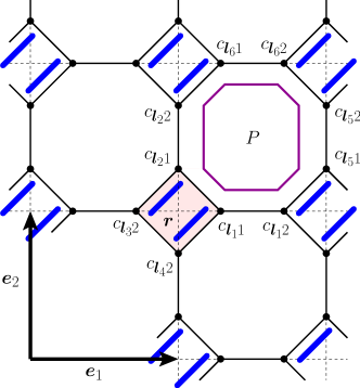
Figure 1: A decorated square lattice (with unit vectors ${\bm{e_{1}}}$ and ${\bm{e_{2}}}$) in which each site is replaced by a tilted square (representing a superconducting grain at site ${\bm{r}}$). Two nanowires (solid blue diagonal lines) are placed on each grain. The grains are coupled to each other via Josephson couplings. A local (gauge) symmetry operator of the model is $G_{P}=(ic_{{\bm{l}}_{1}1}c_{{\bm{l}}_{1}2})(ic_{{\bm{l}}_{5}1}c_{{\bm{l}}_{5}2})(ic_{{\bm{l}}_{6}1}c_{{\bm{l}}_{6}2})(ic_{{\bm{l}}_{2}1}c_{{\bm{l}}_{2}2})$, where $P$ defines the minimal closed loop. See text.

For example, in Fig. 1, two parallel nanowires are placed on each superconducting grain. These grains are placed on the sites ${\bm{r}}$ of a square lattice matrix. The two nanowires on each grain yield four Majorana fermionic degrees of freedom, placed on the edges of the oriented links of the lattice. The Majorana fermions on different superconducting grains, sharing a link, are coupled to each other by Josephson junctions. Prior to introducing the Josephson couplings, each grain is shunted to maintain a fixed superconducting phase and is capacitively coupled to a ground plate. Consequently, there are large fluctuations in the electron number operator. However, the electron number parity is conserved. The sum of the two dominant effects: (i) inter-grain Josephson couplings and (ii) intra-grain constraints on the electron-number parity, complemented by exponentially small capacitive energies, leads to a simple effective Hamiltonian. The intra-grain constraint on electron number (even/odd) parity is more dominant than inter-grain effects. The parity operator is ${\cal P}_{{\bm{r}}}=(-1)^{n_{{\bm{r}}}}$ with $n_{{\bm{r}}}$ the total number of electrons on grain ${\bm{r}}$. This electron number parity can be of paramount importance in interacting Majorana systems. lfu ; xulu In grains having two nanowires each, the electronic parity operator is quartic in the Majorana fermions; it is just the ordered product of the four Majorana fermions at the endpoints of the nanowires on top of the grain at site ${\bm{r}}$,

$${\cal P}_{{\bm{r}}}=c_{{\bm{l}}_{1}1}c_{{\bm{l}}_{2}1}c_{{\bm{l}}_{3}2}c_{{\bm{l}}_{4}2},\ \ \ \ {\bm{r}}\in{\bm{l}}_{1},{\bm{l}}_{2},{\bm{l}}_{3},{\bm{l}}_{4}$$ (1)

(we write ${\bm{r}}\in{\bm{l}}$ to indicate that ${\bm{r}}$ is one of the two endpoints of ${\bm{l}}$). This gives rise to a term in the effective Hamiltonian of the form Terhal

$$H_{0}=-h\sum_{{\bm{r}}}{\cal{P}}_{{\bm{r}}},$$ (2)

with the sum taken over all grains, whose total number is $N_{\bm{r}}$. This term is augmented by Josephson couplings across inter-grain links ${\bm{l}}$, leading to a Majorana Fermi bilinear term involving the coupled pair of Majoranas $\{(c_{{\bm{l}}1},c_{{\bm{l}}2})\}$,

$$H_{1}=-J\sum_{{\bm{l}}}ic_{{\bm{l}}1}c_{{\bm{l}}2}.$$ (3)

Fermionic parity effects are more dominant than Josephson coupling ($h\gg J$) effects. Invoking perturbation theory, for small $(J/h)$, it was found Terhal that, to lowest non-trivial order, the resultant effective Hamiltonian was identical to that of Kitaev’s toric code model, kitaev03 thus establishing that such a system may support TQO. Unfortunately, for $(J/h)\ll 1$, spectral gap is small and the system is more susceptible to thermal fluctuations and noise. A Jordan-Wigner transformation was invoked Terhal to illustrate that these results survive for finite $(J/h)$.

In this article, we will outline a general procedure for the design of different architectures of nanowires on superconducting grains that support TQO. As alluded to above, our considerations will not be limited to the use of perturbation theory but will rather rely on the use of symmetries and exact generalized dualities associated with these granular and other systems defined on general networks. We will further invoke a general framework for dualities that does not require the incorporation of known explicit representations of a spin in terms of Majorana fermions nor Jordan-Wigner transformations that have been invoked in earlier works. xulu ; Terhal ; Fradkin The bond-algebraic approach, ads ; NO ; bond ; orbital ; bondprl ; ADP ; clock that we employ to study general exact dualities and fermionization, bondprl ; ADP allows for the derivation of earlier known dualities as well as a plethora of many new others for rather general networks (or graphs) in arbitrary dimensions and boundary conditions. It is important to note, as we will return to explicitly later, that as Dirac fermions can be expressed as a linear combination of two Majorana fermions, our mappings lead to dualities between standard (non-Majorana) fermionic systems and spin systems on arbitrary graphs in general dimensions. These afford non-trivial examples of fermionization in more that one dimension.

Among several exact dualities that we report here we note, in particular, the following:

• A duality, in any dimension, between the Majorana fermion system corresponding to an arbitrary network of nanowires on superconducting grains and quantum Ising gauge theories.

• A gauge-reducing and emergent dualities ADP in arbitrary number of dimensions between granular Majorana Fermi systems on an arbitrary network and transverse-field Ising models with annealed exchange couplings. In two dimensions, this duality, along with the first one listed above, indicates that an annealed average over a random exchange may leave the system identical to a uniform transverse-field Ising model.

• A further duality between a particular Majorana fermion architecture and a nearest-neighbor quantum spin $S=1/2$ model which, in some sense, is intermediate between an Ising model on a honeycomb lattice and the Kitaev honeycomb model. Kitaev06 We term this system the “XXZ honeycomb compass model”.

As one of the key issues that we wish to address concerns viable TQO, boundary conditions may be of paramount importance. Boundary conditions are inherently related to the character (and, on highly connected systems, to the number) of independent $d$-dimensional gauge-like symmetries. Imposing periodic or other boundary conditions on a system can lead to vexing problems in traditional approaches to dualities and fermionization. By using bond-algebras, we can circumvent these obstacles and construct exact dualities for both infinite systems and for finite systems endowed with arbitrary boundary conditions. Other formidable barricades, such as the use of non-local string transformations, can be overcome as well within the bond-algebraic approach to dualities. ADP The validity of any duality mapping can, of course, be checked numerically by establishing that the spectra of the two purported dual finite systems indeed coincide. The matching of the spectra serves as a definitive test since dualities are (up to global redundancies) unitary transformations ADP that preserve the spectrum of the system.

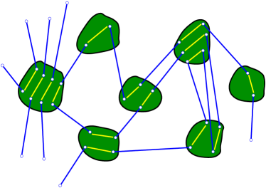
Figure 2: A general network of superconducting grains with an even coordination number of each vertex. The local coordination number $q_{{\bm{r}}}$ of any superconducting grain centered about site ${\bm{r}}$ is equal to the number of endpoints of all nanowires that are placed on that superconducting grain. The dominant Josephson tunneling paths between inter-grain nanowire endpoints are highlighted by solid lines. Shown here is a two-dimensional projection of the network.

II Networks of Superconducting Grains and Nanowires

In the Introduction, we succinctly reviewed the effective Hamiltonian for the square lattice array,Terhal depicted in Fig. 1, of Josephson-coupled granular superconductors carrying each two nanowires. This architecture serves as a useful case of study. There is more to life, however, than square lattice arrays (although we will return to these later on in this work). We consider next rather general architectures in which each node ${\bm{r}}$ (superconducting grain) has an even number of nearest neighbors to which it is linked by Josepshon coupling, see Fig. 2. These general networks include, of course, any two dimensional lattice of even coordination, e.g, those of Figs. 1, and 3, as special cases.

The architectures that we consider are realized by placing at each vertex ${\bm{r}}$ of a graph-theoretical network a finite-size superconducting grain. On each of these grains there are $z_{{\bm{r}}}$ nanowires. These nanowires provide $2z_{{\bm{r}}}$ Majorana fermions, one for each wire’s endpoint. Inter-grain Josephson tunneling is represented by a link involving Majoranas coming from different wires on different islands. We place the nanowires on every grain in the network so that each endpoint of a nanowire is near the endpoint of another nanowire on a neighboring grain, to maximize Josephson tunneling. Thus, the coordination number $q_{{\bm{r}}}$ of grain ${\bm{r}}$ in these graphs is $q_{{\bm{r}}}=2z_{{\bm{r}}}$.combinatorics The general situation is depicted in Fig. 2.

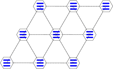
Figure 3: A triangular network of superconducting grains (hexagons) on each of which we place three nanowires.

The basic inter and intra-island interactions have different origins. For ease of reference, we reiterate these below for arbitrary networks:

• there is a Josephson coupling $J_{{\bm{l}}}$ associated with each inter-grain link ${\bm{l}}$ of the network connecting different superconducting grains, and

• an intra-grain charging energy $h_{{\bm{r}}}$ associated to each island at site ${\bm{r}}$.

In a general, spatially non-uniform, network the spatial distribution of couplings $J_{{\bm{l}}}$ and charging energies $h_{{\bm{r}}}$ need not be constant.

The algebra of Majorana fermions is defined by the following relations:

$$\{c_{{\bm{l}}i},c_{{\bm{l}}^{\prime}i^{\prime}}\}=2\delta_{{\bm{l}},{\bm{l}}^{\prime}}\delta_{i,i^{\prime}},\ \ \ \ c_{{\bm{l}}i}^{\dagger}=c_{{\bm{l}}i}.$$ (4)

With all of the above preliminaries in tow,irreps we are now ready to present the effective Hamiltonian for the systems under consideration,

$$H_{\sf M}=-i\sum_{{\bm{l}}}J_{{\bm{l}}}c_{{\bm{l}}1}c_{{\bm{l}}2}-\sum_{{\bm{r}}}h_{{\bm{r}}}{\cal P}_{{\bm{r}}},$$ (5)

where

$${\cal{P}}_{{\bm{r}}}\equiv i^{z_{{\bm{r}}_{2}}}\ c_{{\bm{l}}_{1}i_{1}}c_{{\bm{l}}_{2}i_{2}}\cdots c_{{\bm{l}}_{q_{{\bm{r}}}}i_{q_{{\bm{r}}}}},\ {\bm{r}}\in{\bm{l}}_{1},\cdots,{\bm{l}}_{q_{{\bm{r}}}},$$ (6)

is the product of all Majorana fermion operators associated with the superconducting grain at site ${\bm{r}}$, ordered in some definite but arbitrary fashion (differing orderings produce the same operator up to a sign). order_explain

The index $i_{m}$ can be either $i_{m}=1$ or $i_{m}=2$, depending on the particular orientation that has been assigned to the links in the network. More precisely, $i_{m}=1$ if ${\bm{l}}_{m}$ points away from ${\bm{r}}$, and $i_{m}=2$ if ${\bm{l}}_{m}$ points into ${\bm{r}}$. The factor $i^{z_{{\bm{r}}_{2}}}$ is introduced to render ${\cal P}_{\bm{r}}$ self-adjoint. Since

$$(c_{{\bm{l}}_{1}i_{1}}\cdots c_{{\bm{l}}_{q_{{\bm{r}}}}i_{q_{{\bm{r}}}}})^{\dagger}=(-1)^{q_{\bm{r}}(q_{\bm{r}}-1)/2}c_{{\bm{l}}_{1}i_{1}}\cdots c_{{\bm{l}}_{q_{{\bm{r}}}}i_{q_{\bm{r}}}}$$ (7)

and $q_{\bm{r}}=2z_{\bm{r}}$, we set the integer $z_{{\bm{r}}_{2}}$ to be the number of nanowires counted modulo $2$,

$$z_{{\bm{r}}_{2}}=\left\{\begin{array}[]{lcl}0&\mbox{if}&z_{{\bm{r}}}\ \mbox{is even}\\ 1&\mbox{if}&z_{{\bm{r}}}\ \mbox{is odd}\end{array}\right..$$ (8)

As we remarked earlier, the operators ${\cal{P}}_{{\bm{r}}}$ are related to the operators $n_{{\bm{r}}}$ counting the total number of electrons on the grain ${\bm{r}}$ as

$${\cal P}_{{\bm{r}}}=(-1)^{n_{\bm{r}}},$$ (9)

thus measuring the parity of the number of electrons at site ${\bm{r}}$. Hamiltonian (5) constitutes an arbitrary dimensional generalization of the sum of the two terms in Eqs. (2, 3). In the following, we call the operators $\{ic_{{\bm{l}}1}c_{{\bm{l}}2}\}$ and $\{{\cal{P}}_{\bm{r}}\}$ the bonds of the Hamiltonian $H_{\sf M}$.bondprl ; ADP

III Symmetries and Topological Quantum Order

For the particular case of the square lattice ($D=2$), the interacting Majorana Hamiltonian $H_{\sf M}$ with periodic (toroidal) boundary conditions was found to exhibit $0$-dimensional local, $d=1$-dimensional gauge-like, and $2$-dimensional global symmetries. Terhal These symmetries, inherently tied to TQO TQO and dimensional reduction, TQO ; BN ; ads also appear in the more general network renditions of the granular system just described in the previous section. They are also manifest for the interacting Majorana systems embedded in any spatial dimension $D\geq 2$ when different boundary conditions are imposed.topology

Global Symmetry:
The Hamiltonian $H_{\sf M}$ of Eq. (5) displays a global symmetry $Q$, given by the product of all the Majorana Fermion operators in the system. We can write $Q$ in terms of bonds as

$$Q=\prod_{\bm{r}}{\cal P}_{\bm{r}},$$ (10)

since each Majorana is contributed by some island. The order of the bonds in $Q$ is not an issue, since

$$[{\cal P}_{\bm{r}},{\cal P}_{{\bm{r}}^{\prime}}]=0,$$ (11)

for any pair of sites ${\bm{r}},{\bm{r}}^{\prime}$. The conserved charge $Q$ represents a $\mathbb{Z}_{2}$ symmetry of the system,

$$Q^{2}=\mathds{1}.$$ (12)

Beyond this global symmetry, the system of Eq. (5) exhibits independent symmetries that operate on finer, lower-dimensional regions of the network. Of particular importance to TQO are $d=1$ and $d=0$-dimensional symmetries, and so we turn to these next.

$d=1$ symmetries:
The $d=1$ dimensional symmetry operators of the Majorana system are given by

$$Q_{\ell}=\prod_{{\bm{l}}\in\ell}(ic_{{\bm{l}}1}c_{{\bm{l}}2}),\ \ \ \ (Q_{\ell})^{2}=\mathbb{1},$$ (13)

where $\ell$ is a continuous contour, finite or infinite and open or closed depending on boundary conditions, entirely composed of links. That these non-local operators are symmetries is readily seen once it is noted that (a) each of the terms (or bonds) in the summand of Eq. (5) defining $H_{\sf M}$ involves products of an even number of Majorana fermions and (b) by the second of Eqs. (4), effecting an even number of permutations of Majorana fermion operators in a product incurs no sign change. For example, for a network of linear dimension $L$ along a Cartesian axis, the contour $\ell$ spans ${\cal{O}}(L^{1})$ sites and is thus a $d=1$ dimensional object. This is the origin of the name $d=1$ symmetries. Some of these $d=1$ symmetries may be related to (appear as products of) the local symmetries discussed next, depending on the topology enforced by boundary conditions. Some others are fundamental and cannot be expressed in terms of those local symmetries.

$d=0$ symmetries:
For the models under consideration, local, also called gauge, $d=0$ symmetries are associated with the elementary loops (or plaquettes) $P$ of the wires, see Fig. 1 for an example. That is, when considering the superconductors as point nodes, the links ${\bm{l}}$ form a network with minimal closed loops $P$. The associated local symmetries are given by

$$G_{P}=\prod_{{\bm{l}}\in P}(ic_{{\bm{l}}1}c_{{\bm{l}}2}),\ \ \ \ G_{P}^{2}=\mathds{1}.$$ (14)

Repeating the considerations of (a) and (b) above, we see that, for any elementary plaquette $P$, the product of Majorana Fermi operators in Eq. (14) commutes with $H_{\sf M}$, since it shares an even number (possibly zero) of Majorana fermions with any bond in the Hamiltonian. By multiplying operators $G_{P}$ for a collection of plaquettes $P$ that, together, tile a region bounded by the loop $\Gamma$, it is readily seen that this product is also a symmetry, as in standard theories with gauge symmetries.

The symmetries above lead to non-trivial consequences:

(A) By virtue of Elitzur’s theorem Elitzur and its $d>0$ generalizations TQO ; BN ; ads all non-vanishing correlators $\langle\prod_{\alpha\in S}c_{\alpha}\rangle$ with $S$ a set of sites $\alpha$ must be invariant under all of the symmetries of Eqs. (13,14). That is, $d=0,1$-gauge-like symmetries cannot be spontaneously broken. As we alluded to earlier, one consequence of the non-local symmetries such as the $d=1$ symmetries of Eq. (13) is the existence of TQO. TQO ; topology

(B) Bounds on autocorrelation times. As a consequence of the $d=1$ symmetries of Eq. (13), and the aforementioned generalization of Elitzur’s theorem as it pertains to temporal correlators, ads the Majorana Fermi system will exhibit finite autocorelation times regardless of the system size. Of course, for various realizations of dynamics and geometry of the disorder, different explicit forms of the autocorrelation times can be found. For instance, by use of bond-algebras, Kitaev’s toric code model is identical to that of a classical square plaquette model as in Ref. auto, . Similarly, Kitaev’s toric code model kitaev03 can be mapped onto two uncoupled one-dimensional Ising chains. bond ; NO ; TQO Different realizations of the dynamics can lead to different explicit forms of $\tau$ in both cases, however, finite autocorrelation times are found in all cases (as they must be). Similarly, more general than the exact bond algebraic mapping and dimensional reductions that we find here, by virtue of $d=1$ symmetries of Eq. (13), autocorrelation functions involving Majorana fermions on a line $\ell$ must be bounded by corresponding ones in a $d=1$ dimensional system. ads

IV Dualities and spin realizations of arbitrary Majorana Architectures

In this Section, we provide two spin duals to the interacting Majorana system described by the effective Hamiltonian $H_{\sf M}$ of Eq. (5) on arbitrary lattices/networks. This applies to finite or infinite systems and for arbitrary boundary conditions. These two dual systems are (1) quantum Ising gauge theories for $D=2$ systems, and more general spin gauge theories in higher-dimensions, and (2) a family of transverse-field Ising models with annealed disorder in the exchange couplings (each model representing a single gauge sector of $H_{\sf M}$). The dualities will be established in the framework of the theory of bond algebras of interactions, bondprl ; ADP as it applies to the study of general dualities between many-body Hamiltonians. The general bond algebraic method relies on a comparison of the algebras, in the respective two dual model, that are generated by the corresponding local interaction terms (or bonds) in these theories. ads ; NO ; bond ; orbital ; bondprl ; ADP ; clock For the problem at hand, the Hamiltonian $H_{\sf M}$ is built as the sum of two sets of Hermitian bonds

$$ic_{{\bm{l}}1}c_{{\bm{l}}2},\ {\cal P}_{\bm{r}},$$ (15)

where ${\bm{l}}$ and ${\bm{r}}$ are links and sites of the network supporting $H_{\sf M}$ (${\cal P}_{\bm{r}}$ was defined in Eq. (6)). In this paper, we will only consider the bond algebra ${\cal A}_{\sf M}$ generated by these bonds. We can then obtain dual representations of $H_{\sf M}$ by looking for alternative local representations of ${\cal A}_{\sf M}$. But first we have to characterize ${\cal A}_{\sf M}$ in terms of relations.

The problem of characterizing a bond algebra of interactions is simplified by several features brought about by physical considerations of locality. The first consequence of locality is that interactions are sparse, meaning that each bond in any local Hamiltonian commutes with most other bonds and is involved in only a small number of relations (or constraints) that link individual bonds to one another. Hence the number of non-trivial relations per bond is small. The second consequence is that relations in a bond algebra can be classified into intensive and extensive, and most relations are intensive. We call a relation intensive if the number of bonds it involves is independent of the size of the system, and extensive if the numbers of bonds it involves scales with the size of the system. Since extensive relations could potentially lead to unphysical non-local behavior, they are typically few in number and may reflect the topology of the system regulated by the boundary conditions, as we will illustrate repeatedly in this paper. As there are $(2z_{\bm{r}})$ Majorana modes (or, equivalently, $z_{\bm{r}}$ fermionic modes) per grain, the Majorana theory of Eq. (5) and the algebraic relations listed above are defined on a Hilbert space of dimension $\dim{\cal{H}}_{\sf M}=2^{z_{{\bm{r}}}N_{{\bm{r}}}}$

Next, we characterize the bond algebra ${\cal A}_{\sf M}$ as the first step toward the construction of its spin duals. The intensive relations are:

1. for any ${\bm{r}}$ and ${\bm{l}}$

   $$(ic_{{\bm{l}}1}c_{{\bm{l}}2})^{2}=\mathds{1}=({\cal P}_{\bm{r}})^{2},$$ (16)

2. for ${\bm{r}},{\bm{r}}^{\prime}\in{\bm{l}}$,

   $$\{{\cal P}_{\bm{r}},ic_{{\bm{l}}1}c_{{\bm{l}}2}\}=0=\{{\cal P}_{{\bm{r}}^{\prime}},ic_{{\bm{l}}1}c_{{\bm{l}}2}\},$$ (17)

3. for ${\bm{r}}\in{\bm{l}}_{i},\ i=1,2,\cdots,q_{\bm{r}}$,

   $$\{{\cal P}_{\bm{r}},ic_{{\bm{l}}_{i}1}c_{{\bm{l}}_{i}2}\}=0.$$ (18)

Thus in the bulk, or everywhere for periodic boundary conditions, each island anticommutes with four $q_{\bm{r}}$ (the coordination of ${\bm{r}}$) links, and each link anticommutes with two islands. The presence or absence of extensive relations depends on the boundary conditions. For periodic (toroidal) or other closed boundary conditions (e.g., spherical), we have one extensive relation

$$\prod_{\bm{r}}{\cal P}_{\bm{r}}=\alpha\prod_{\bm{l}}(ic_{{\bm{l}}1}c_{{\bm{l}}2}),\ \ \ \ \alpha=\pm 1,$$ (19)

since each Majorana Fermion operator appears exactly once both on the left and right-hand side of this equation, but not necessarily in the same order. The constant $\alpha$ adjusts for the potentially different orderings, and the overall powers of $i$ on each side of the equation. Notice that $\prod_{\bm{r}}{\cal P}_{\bm{r}}=Q$ is the global $\mathds{Z}_{2}$ symmetry operator. In contrast, for open or semi-open (e.g., cylindrical) boundary conditions, the islands on the free boundary have Majorana fermions that are not matched by links (that is, that do not interact with Majoranas on other islands). Hence the product

$$\left(\prod_{\bm{r}}{\cal P}_{\bm{r}}\right)\left(\prod_{\bm{l}}(ic_{{\bm{l}}1}c_{{\bm{l}}2})\right)=B$$ (20)

reduces to the product $B$ of these Majoranas on the free boundary. The operator $B$ may or may not commute with the Hamiltonian, depending on the details of the architecture at the boundary, see Fig. 4, but either way Eq. (20) does not represent an extensive relation in the bond algebra (rather it just states how to write a particular operator as a product of bonds). If $[H_{\sf M},B]=0$, $B$ represents a $\mathds{Z}_{2}$ boundary symmetry independent of the local symmetries.

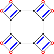
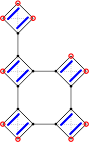
Figure 4: Two architectures with open boundary conditions. In either case, the operator $B$ of Eq. (20) is the product of all the uncoupled Majoranas on the boundary indicated by open circles, but $[H_{\sf M},B]=0$ only for the system shown in the panel on the left.

IV.1 Duality to quantum Ising gauge theories

In this Section we describe a duality relating the Hamiltonian $H_{\sf M}$ to a system of $S=1/2$ spins. The spin degrees of freedom are placed on the (center of the) links of a network identical to the one associated to $H_{\sf M}$, and are described by Pauli matrices $\sigma^{x}_{\bm{l}},\sigma^{y}_{\bm{l}},\sigma^{z}_{\bm{l}}$. The goal is to introduce interactions among these spins that satisfy the same algebraic relations as the bonds of $H_{\sf M}$. Let us introduce the Hermitian spin bond

$${\widetilde{\cal{P}}}_{\bm{r}}=\prod_{\{{\bm{l}}|{\bm{r}}\in{\bm{l}}\}}\sigma^{z}_{\bm{l}}.$$ (21)

For example, for the special case of the square lattice discussed in the Introduction,

$${\widetilde{\cal{P}}}_{\bm{r}}=\sigma^{z}_{{\bm{l}}_{1}}\sigma^{z}_{{\bm{l}}_{2}}\sigma^{z}_{{\bm{l}}_{3}}\sigma^{z}_{{\bm{l}}_{4}},\ \ \ \ {\bm{r}}\in{\bm{l}}_{1},{\bm{l}}_{2},{\bm{l}}_{3},{\bm{l}}_{4}.$$ (22)

The set of spin bonds

$$\sigma^{x}_{\bm{l}},\ \ \ \ \widetilde{\cal P}_{\bm{r}},$$ (23)

satisfy the following intensive relations

1. for any ${\bm{r}}$ and ${\bm{l}}$

   $$(\sigma^{x}_{\bm{l}})^{2}=\mathds{1}=(\widetilde{\cal P}_{\bm{r}})^{2},$$ (24)

2. for ${\bm{r}},{\bm{r}}^{\prime}\in{\bm{l}}$,

   $$\{\widetilde{\cal P}_{\bm{r}},\sigma^{x}_{\bm{l}}\}=0=\{\widetilde{\cal P}_{{\bm{r}}^{\prime}},\sigma^{x}_{\bm{l}}\},$$ (25)

3. for ${\bm{r}}\in{\bm{l}}_{i},\ i=1,2,\cdots,q_{\bm{r}}$,

   $$\{\widetilde{\cal P}_{\bm{r}},\sigma^{x}_{{\bm{l}}_{i}}\}=0,$$ (26)

everywhere for closed boundary conditions, and everywhere in the bulk for open or semi-open boundary conditions. These relations are identical to the intensive relations for the bonds of $H_{\sf M}$. In the Ising gauge theory, the bond algebraic relations listed above are defined on a space of size $2^{z_{r}N_{{\bm{r}}}}$. (That this is so can be easily seen by noting that there are $N_{{\bm{l}}}=z_{{\bm{r}}}N_{{\bm{r}}}$ links each endowed with a spin $S=1/2$ degree of freedom $\sigma^{z}_{\bm{l}}$.) As it so happens, this Hilbert space dimension is identical to that of the Majorana system of $H_{\sf M}$. Putting all of the pieces together, we see that the spin Hamiltonian

$$H_{\sf QIG}=-\sum_{{\bm{l}}}J_{{\bm{l}}}\sigma^{x}_{\bm{l}}-\sum_{{\bm{r}}}h_{{\bm{r}}}\widetilde{\cal P}_{\bm{r}}$$ (27)

is unitarily equivalent to $H_{\sf M}$, provided the extensive relations are matched as well. For open or semi-open boundary conditions, the same follows provided that the intensive relations on the boundary also properly match. In the following, we focus on periodic boundary conditions (of theoretical interest in connection to TQO), and leave the discussion of open boundary conditions (of interest for potential experimental realizations of these systems) to the Appendix A.

As just explained, the mapping of bonds

$$ic_{{\bm{l}}1}c_{{\bm{l}}2}\mapsto\sigma^{x}_{\bm{l}},\ \ \ \ {\cal P}_{\bm{r}}\mapsto\widetilde{\cal P}_{\bm{r}}$$ (28)

preserves the intensive algebraic relations. In particular it maps the local symmetries of Eq. (14) to local symmetries of $H_{\sf QIG}$,

$$G_{P}\equiv\prod_{{\bm{l}}\in P}(ic_{{\bm{l}}1}c_{{\bm{l}}2})\mapsto\prod_{{\bm{l}}\in P}\sigma^{x}_{\bm{l}}\equiv G_{S,P}.$$ (29)

To assess the effect it has on the extensive relation of Eq. (19) (and the global symmetry), notice that (for periodic boundary conditions)

$$\prod_{\bm{l}}(ic_{{\bm{l}}1}c_{{\bm{l}}2})\mapsto\prod_{\bm{l}}\sigma^{x}_{\bm{l}}\equiv Q_{S}$$ (30)

with $[Q_{S},H_{\sf QIG}]$ a global symmetry of $H_{\sf QIG}$, and

$$\prod_{\bm{r}}{\cal P}_{\bm{r}}\mapsto\prod_{\bm{r}}\widetilde{\cal P}_{\bm{r}}=\mathds{1}.$$ (31)

It follows that, as it stands, the mapping of bonds of Eq. (28) is a correspondence, but not an isomorphism of bond algebras. The simplest way to convert it into an isomorphism is to modify one and only one of the bonds $\widetilde{\cal P}_{\bm{r}}$ of the spin model at some arbitrary site ${\bm{r}}_{0}$, so that

$$\widetilde{\cal P}_{{\bm{r}}_{0}}\equiv\alpha Q_{S}\prod_{\{{\bm{l}}|{\bm{r}}_{0}\in{\bm{l}}\}}\sigma^{z}_{\bm{l}}$$ (32)

($\alpha$ was defined in Eq. (19)) while for any other site ${\bm{r}}\neq{\bm{r}}_{0}$, $\widetilde{\cal P}_{{\bm{r}}}$ remains unchanged. The introduction of this modified bond does not change the intensive relations, since $Q_{S}$ commutes with every bond (original or modified). Moreover,

$$\prod_{\bm{r}}{\cal P}_{\bm{r}}\mapsto\widetilde{\cal P}_{{\bm{r}}_{0}}\prod_{{\bm{r}}\neq{\bm{r}}_{0}}\widetilde{\cal P}_{\bm{r}}=\alpha Q_{S}$$ (33)

and the extensive relation of Eq. (19) is now, with the modified definition of $\widetilde{\cal P}_{{\bm{r}}_{0}}$, preserved, since ($\alpha^{2}=1$)

$$\prod_{\bm{l}}\sigma^{x}_{\bm{l}}=\alpha\widetilde{\cal P}_{{\bm{r}}_{0}}\prod_{{\bm{r}}\neq{\bm{r}}_{0}}\widetilde{\cal P}_{\bm{r}}.$$ (34)

Hence there is a unitary transformation $\mathcal{U}_{{\sf d}}$ such that

$$\mathcal{U}_{{\sf d}}H_{\sf M}\mathcal{U}_{{\sf d}}^{\dagger}=H_{\sf QIG},$$ (35)

with $H_{\sf QIG}$ containing the single modified bond $\widetilde{\cal P}_{{\bm{r}}_{0}}$.

In the duality between the systems of Eqs. (5, 27), the dimensions of the their Hilbert spaces are identical. Since we count two Majorana modes (or, equivalently, one Fermionic mode) per link, the Hamiltonian $H_{\sf M}$ is defined on a Hilbert space of dimension $\dim{\cal{H}}_{\sf M}=2^{N_{{\bm{l}}}}$, with $N_{{\bm{l}}}$ denoting the total number of links in the network. On the other hand, the spin system has one spin $S=1/2$ degree of freedom per link, hence the dimension of the Hilbert space on which $H_{\sf QIG}$ is defined is also $2^{N_{{\bm{l}}}}$. Notice that the need to introduce the modified bond $\widetilde{\cal P}_{{\bm{r}}_{0}}$ in the dual spin theory is irrelevant from the point of exploiting the duality to study the ground-state properties of $H_{\sf M}$ (or viceversa, to study the ground-state properties of $H_{\sf QIG}$), since for finite systems the ground state $|\Omega\rangle$ must satisfy $Q_{S}|\Omega\rangle=|\Omega\rangle$. The ease with which we established the duality between Majorana systems and QIG systems for general lattices and networks illustrates how efficient the bond-algebraic construct is.

The duality just described is extremely general, valid in particular for any number of space dimensions $D$. In the following we describe explicitly one particularly important special instance, that of $D=2$. On a square lattice, the Hamiltonian $H_{\sf M}$ simplifies to

$$H_{\sf M}=-\sum_{\bm{l}}J_{\bm{l}}(ic_{{\bm{l}}1}c_{{\bm{l}}2})-\sum_{\bm{r}}h_{\bm{r}}c_{{\bm{l}}_{1}1}c_{{\bm{l}}_{2}1}c_{{\bm{l}}_{3}2}c_{{\bm{l}}_{4}2},$$ (36)

where ${\bm{l}}_{1},{\bm{l}}_{2},{\bm{l}}_{3},{\bm{l}}_{4}$ are shown in Fig. 1. This generalizes the Hamiltonian considered in Ref. Terhal, only in that inhomogeneous couplings are allowed. The dual spin (finite-size) system is (${\bm{r}}_{0}\in{\bm{l}}_{0,1},{\bm{l}}_{0,2}{\bm{l}}_{0,3}{\bm{l}}_{0,4}$)

$$H_{\sf QIG}=-h_{{\bm{r}}_{0}}\alpha Q_{S}\sigma^{z}_{{\bm{l}}_{0,1}}\sigma^{z}_{{\bm{l}}_{0,2}}\sigma^{z}_{{\bm{l}}_{0,3}}\sigma^{z}_{{\bm{l}}_{0,4}}-\sum_{{\bm{r}}\neq{\bm{r}}_{0}}h_{\bm{r}}\sigma^{z}_{{\bm{l}}_{1}}\sigma^{z}_{{\bm{l}}_{2}}\sigma^{z}_{{\bm{l}}_{3}}\sigma^{z}_{{\bm{l}}_{4}}-\sum_{\bm{l}}J_{\bm{l}}\sigma^{x}_{\bm{l}}$$ (37)

that we recognize as the standard, $D=2$, $\mathds{Z}_{2}$ Ising gauge theory, fradkin_susskind up to the modified bond at ${\bm{r}}_{0}$ ($Q_{S}=\prod_{\bm{l}}\sigma^{x}_{\bm{l}}$ and $\alpha$ is determined according to Eq. (19)), see Fig. 5.

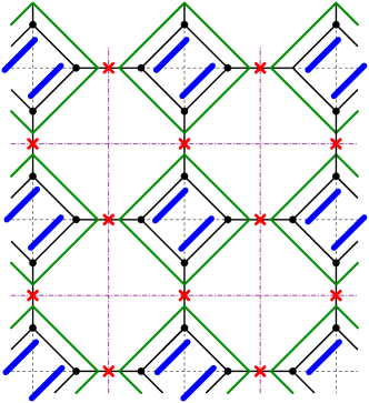
Figure 5: Duality to a $D=2$ $\mathds{Z}_{2}$ quantum Ising gauge theory, where spins are represented as crosses. Hamiltonian $H_{\sf M}$ of Eq. (36) represents a particular fermionization of the $H_{\sf QIG}$ gauge theory.

Hence, we may regard the Hamiltonian of Eq. (36) as an exact fermionization of the $\mathds{Z}_{2}$ Ising gauge theory with periodic boundary conditions (and one modified bond). It is interesting to compare this fermionization with a slightly different one Fradkin that exploits the Jordan-Wigner transformation in the limit of infinite size. This approach yields the Majorana Hamiltonian Fradkin (in our notation)

$$H_{\sf FSS}=-\sum_{\bm{l}}J_{\bm{l}}(ic_{{\bm{l}}1}c_{{\bm{l}}2})-\sum_{\bm{r}}h_{\bm{r}}c_{{\bm{l}}_{1}2}c_{{\bm{l}}_{5}1}c_{{\bm{l}}_{6}2}c_{{\bm{l}}_{2}1},$$ (38)

where ${\bm{l}}_{1},{\bm{l}}_{2},{\bm{l}}_{5},{\bm{l}}_{6}$ are shown in Fig. 1. The two-body interaction $c_{{\bm{l}}_{1}2}c_{{\bm{l}}_{5}1}c_{{\bm{l}}_{6}2}c_{{\bm{l}}_{2}1}$ is different than the two-body interaction in $H_{\sf M}$, since it involves three different islands, see Fig. 6. Hence, disregarding boundary conditions, we see that the $\mathds{Z}_{2}$ quantum Ising gauge theory admits rather different but equivalent fermionizations. As expected, the bonds in $H_{\sf FSS}$ satisfy intensive relations identical to those already discussed for $H_{\sf M}$ and $H_{\sf QIG}$.

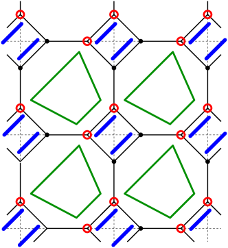
Figure 6: Jordan-Wigner fermionization of the $\mathds{Z}_{2}$ Ising gauge theory realizes a theory of Majorana fermions $H_{\sf FSS}$, with two-body interactions between Majoranas (shown as trapezoids) on three different islands. Notice that, unlike the intra-island two-body interactions of $H_{\sf M}$, two neighboring two-body interactions $H_{\sf FSS}$ share a Majorana operator.

Thus far, we focused on periodic boundary conditions. We now remark on other boundary conditions. When antiperiodic boundary conditions are imposed in a network with an an outer perimeter that includes twice an odd number of links, the right-hand side of Eq. (31) is replaced by $-\mathds{1}$. The union of both cases (periodic and antiperiodic) for a system having a twice odd perimeter spans all possible values of the product $\prod_{{\bm{r}}}\widetilde{{\cal{P}}}_{{\bm{r}}}$. Thus, for these systems in the case of periodic boundary conditions, the spectrum of the Majorana system can be mapped to the union of levels found for the QIG systems for both periodic or antiperiodic boundary conditions. In terms of the corresponding partition functions, we have that

$${\cal{Z}}_{\sf M,\,periodic}={\cal{Z}}_{\sf QIG,\,periodic}+{\cal{Z}}_{\sf QIG,\,antiperiodic}.$$ (39)

IV.2 Duality to annealed transverse-field Ising models

We next derive, in a similar spirit, a duality between the general architecture Majorana system $H_{\sf M}$ and annealed transverse-field Ising models. The number of annealed disorder variables in these systems (along with the number of sites $N_{{\bm{r}}}$) determines the size of the Hilbert space on which the Ising models are defined. With an eye towards things to come, we note (as we will re-iterate later on) that the duality that we will derive in this Section will furnish an example in which the Hilbert space dimensions of two dual systems need not be identical to one another. Generally, dualities are unitary transformations between two theories up to trivial gauge redundancies that do not preserve the Hilbert space dimension. ADP That is, dualities are isometries.

To define the annealed transverse field Ising systems, we place an $S=1/2$ spin on each site ${\bm{r}}$, $\sigma^{x}_{\bm{r}},\sigma^{y}_{\bm{r}},\sigma^{z}_{\bm{r}}$, of the network associated to $H_{\sf M}$, and a classical annealed disorder variable $\eta_{{\bm{l}}}=\pm 1$ on each link ${\bm{l}}$. Then we can introduce the set of Hermitian spin bonds

$$\sigma^{x}_{{\bm{r}}},\ \ \ \ \ \ \ \ \eta_{\bm{l}}\sigma^{z}_{{\bm{r}}}\sigma^{z}_{{{\bm{r}}^{\prime}}},\ \ {\bm{r}},{\bm{r}}^{\prime}\in{\bm{l}}.$$ (40)

If we specialize to periodic boundary conditions, these bonds satisfy a set of intensive relations identical to the ones discussed in the two previous Sections, together with one new relation absent before and listed last below:

1. for any ${\bm{r}}$ and ${\bm{l}}$

   $$(\sigma^{x}_{{\bm{r}}})^{2}=\mathds{1}=(\eta_{\bm{l}}\sigma^{z}_{{\bm{r}}}\sigma^{z}_{{{\bm{r}}^{\prime}}})^{2},$$ (41)

2. for ${\bm{r}},{\bm{r}}^{\prime}\in{\bm{l}}$

   $$\{\sigma^{x}_{{\bm{r}}},\eta_{\bm{l}}\sigma^{z}_{{\bm{r}}}\sigma^{z}_{{\bm{r}}^{\prime}}\}=0=\{\sigma^{x}_{{\bm{r}}^{\prime}},\eta_{\bm{l}}\sigma^{z}_{{\bm{r}}}\sigma^{z}_{{\bm{r}}^{\prime}}\},$$ (42)

3. for ${\bm{r}}\in{\bm{l}}_{i},\ i=1,2,\cdots,q_{\bm{r}}$,

   $$\{\sigma^{x}_{{\bm{r}}},\eta_{{\bm{l}}_{i}}\sigma^{z}_{{\bm{r}}}\sigma^{z}_{{\bm{r}}_{i}^{\prime}}\}=0,\ \ \ \ {\bm{r}}\neq{\bm{r}}_{i}^{\prime}\in{\bm{l}}_{i},$$ (43)

4. for any elementary loop $P$ in the network,

   $$\prod_{{\bm{l}}\in P}(\eta_{\bm{l}}\sigma^{z}_{{\bm{r}}}\sigma^{z}_{{\bm{r}}^{\prime}})=\mathds{1}\prod_{{\bm{l}}\in P}\eta_{\bm{l}}.$$ (44)

The constraint of Eq. (44) holds true for any closed loop. For this reason, and others related to TQO, it is important to clarify the meaning of elementary loop.

Loops in the network that share some links can be joined along those links to obtain another loop or sum of disjoint loops. This means that the set of all loops has a minimal set of generators from which we can obtain any loop or systems of loops by the joining operation just described. We call the loops in an arbitrary but fixed minimal generating set elementary loops. In this way, we obtain a minimal description of the constraints embodied in Eq. (44). It is not obvious a priori whether one should classify these constraints (that is, relations) as intensive or extensive. This depends on the topology of the system. If the system is simply connected, every loop is contractible to some trivial minimal (that is, of minimal length) loop, and hence we can choose minimal loops as elementary loops. These loops afford an intensive characterization of the constraints embodied in Eq. (44). If on the other hand the system is not simply connected, as for periodic boundary conditions, the generating set of elementary loops will include non-contractible loops, and the length of some of these non-contractible loops may scale with the size of the system. Consider, for example, the spin bonds of Eq. (40) on a planar network on the torus and on a punctured infinite plane. Both networks fail to be simply connected, but only the torus forces some of the constraint of Eq. (44) to be extensive, because its two non-contractible loops must scale with the size of the system.

For periodic boundary conditions, there is one extensive relation satisfied by the bonds of Eq. (40),

$$\prod_{\bm{l}}(\eta_{\bm{l}}\sigma^{z}_{\bm{r}}\sigma^{z}_{{\bm{r}}^{\prime}})=\eta\mathds{1},$$ (45)

with

$$\eta\equiv\prod_{\bm{l}}\eta_{\bm{l}},\ \ \ \ \eta=\pm 1,$$ (46)

that may or may not be independent of the relations of Eq. (44), depending on the details of the network. In the following, we will treat it as an independent relation, since it does not affect our results if it turns out to be dependent.

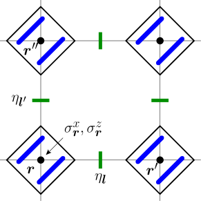
Figure 7: Duality to an annealed transverse-field Ising model, in the particular $D=2$ case. Spins $S=1/2$ are located at the vertices ${\bm{r}}$ of the square lattice and classical $\mathbb{Z}_{2}$ fields $\eta_{\bm{l}}$ at the links ${\bm{l}}$ (indicated by a dash).

It follows that the mapping of bond algebras

$$ic_{{\bm{l}}1}c_{{\bm{l}}2}\mapsto\eta_{\bm{l}}\sigma^{z}_{\bm{r}}\sigma^{z}_{{\bm{r}}^{\prime}},\ \ \ \ {\cal P}_{\bm{r}}\mapsto\sigma^{x}_{\bm{r}},$$ (47)

preserves every local anticommutation relation. Hence the Hamiltonian theory

$$H_{\sf AI}\{\eta_{{\bm{l}}}\}=-\sum_{{\bm{l}}}J_{{\bm{l}}}(\eta_{{\bm{l}}}\sigma^{z}_{\bm{r}}\sigma^{z}_{{\bm{r}}^{\prime}})-\sum_{{\bm{r}}}h_{\bm{r}}\sigma^{x}_{\bm{r}},$$ (48)

obtained from applying this mapping to $H_{\sf M}$ will be shown to be dual to $H_{\sf M}$ (see Fig. 7). The Hilbert space on which the theory of Eq. (48) is defined is of size $\dim{\cal{H}}_{\sf AI}=2^{N_{{\bm{r}}}+N_{\eta}}$ where $N_{{\bm{r}}}$ is the number of superconducting grains and $N_{\eta}$ the total number of $\eta_{\bm{l}}$ fields.

The proposed duality raises an immediate question: What are the features of $H_{\sf M}$ that determine or at least constrain the classical fields $\eta_{\bm{l}}$? As we will see, the answer lies in the local and gauge-like symmetries that $H_{\sf M}$ possesses and $H_{\sf AI}$ lacks. To understand this better, we need to study the effect this mapping has on relations beyond local anticommutation. Let us consider first its effect on the extensive relation of Eq. (19). We have that

$$Q=\prod_{\bm{r}}{\cal P}_{\bm{r}} \mapsto \prod_{\bm{r}}\sigma^{x}_{\bm{r}}=Q_{S},$$ (49)

$$\alpha\prod_{\bm{l}}(ic_{{\bm{l}}1}c_{{\bm{l}}2}) \mapsto \alpha\prod_{\bm{l}}(\eta_{\bm{l}}\sigma^{z}_{\bm{r}}\sigma^{z}_{{\bm{r}}^{\prime}})=\alpha\eta\mathds{1}.$$ (50)

As for periodic boundary conditions the left-hand sides of Eqs. (49) and (50) represent the same operator, but the right-hand sides are different operators, the mapping as it stands does not preserve the relation of Eq. (19). We know of a solution to this shortcoming from the previous Section. If we modify one and only one bond placed on some fixed but arbitrary link ${\bm{l}}_{0}$ to read

$$\alpha\eta\eta_{{\bm{l}}_{0}}\sigma^{z}_{\bm{r}}\sigma^{z}_{{\bm{r}}^{\prime}}Q_{S},$$ (51)

then

$$\alpha\prod_{\bm{l}}(ic_{{\bm{l}}1}c_{{\bm{l}}2})\mapsto$$

$$\alpha^{2}(\eta\eta_{{\bm{l}}_{0}}\sigma^{z}_{{\bm{r}}_{0}}\sigma^{z}_{{{\bm{r}}_{0}}^{\prime}})Q_{S}\prod_{{\bm{l}}\neq{\bm{l}}_{0}}(\eta_{\bm{l}}\sigma^{z}_{\bm{r}}\sigma^{z}_{{\bm{r}}^{\prime}})=Q_{S},$$ (52)

as required by Eq. (19).

The presence of the modified bond at ${\bm{l}}_{0}$ introduces a new feature into the discussion leading to Eq. (44). Now we have that, for any elementary loop $P$,

$$\prod_{{\bm{l}}\in P}(\eta_{\bm{l}}\sigma^{z}_{\bm{r}}\sigma^{z}_{{\bm{r}}^{\prime}})=\left\{\begin{array}[]{lcr}\mathds{1}\prod_{{\bm{l}}\in P}\eta_{\bm{l}},&\ \ \mbox{if}&{\bm{l}}_{0}\not\in P,\\ \\ \alpha\eta Q_{S}\prod_{{\bm{l}}\in P}\eta_{\bm{l}}&\ \ \mbox{if}&{\bm{l}}_{0}\in P.\end{array}\right.$$ (53)

If we consider the role of the elementary loops $P$ in the Majorana system $H_{\sf M}$, and consider the mapping of Eq. (40), we see that the local symmetries (see Section III)

$$G_{P}\equiv\prod_{{\bm{l}}\in P}(ic_{{\bm{l}}1}c_{{\bm{l}}2})$$ (54)

of $H_{\sf M}$ are mapped to one of the two possibilities listed in Eq. (53), showing that as it stands, the mapping of Eq. (40) is still not an isomorphism of bond algebras. The problem is that a large number of distinct symmetries are being mapped either to a trivial symmetry (a multiple of the identity operator), or a multiple of the global $\mathds{Z}_{2}$ symmetry $Q_{S}$ of the annealed Ising model. We can fix this problem by decomposing the Hamiltonians $H_{\sf M}$ and $H_{\sf AI}$ into their symmetry sectors, where the obstruction to the duality mapping disappears. Thus we are able to establish emergent dualities,bondprl ; ADP that is, dualities that emerge between sectors of the two theories.

The sector decomposition is simple for $H_{\sf AI}$, that has only one symmetry $Q_{S}$, with eigenvalues $q_{S}=\pm 1$. Then we can decompose the Hilbert space ${\cal H}_{\sf AI}$ as

$${\cal H}_{\sf AI}=\bigoplus_{q_{S}=\pm 1}{\cal H}_{q_{S}},$$ (55)

so that if $\Lambda_{q_{S}}$ is the orthogonal projector onto ${\cal H}_{q_{S}}$, then

$$Q_{S}\Lambda_{q_{S}}=\pm\Lambda_{q_{S}}.$$ (56)

For $H_{\sf M}$, since its symmetries form a commuting set, one can simultaneously diagonalize them and break the Hilbert space ${\cal H}_{\sf M}$ into sectors labelled by the symmetries’ simultaneous eigenvalues, $q=\pm 1$ for the global symmetry and $\Gamma_{P}=\pm 1$ for the loop symmetries:

$${\cal H}_{\sf M}=\bigoplus_{q,\{\Gamma_{P}\}}{\cal H}_{q,\{\Gamma_{P}\}}.$$ (57)

The Hamiltonian $H_{\sf M}$ is block-diagonal relative to this decomposition, and, if $\Lambda_{q,\{\Gamma_{P}\}}$ is the orthogonal projector onto the subspace ${\cal H}_{q,\{\Gamma_{P}\}}$, we have that

$$Q\Lambda_{q,\{\Gamma_{P}\}} = q\Lambda_{q,\{\Gamma_{P}\}},$$ (58)

$$G_{P}\Lambda_{q,\{\Gamma_{P}\}} = \Gamma_{P}\Lambda_{q,\{\Gamma_{P}\}},$$ (59)

for any elementary loop $P$.

The problem now is to decide which choice of sectors will make the projected Hamiltonians $H_{\sf M}\Lambda_{q,\{\Gamma_{P}\}}$ and $H_{\sf AI}\Lambda_{q_{S}}$ dual to each other. From Eqs. (49), and (53), we obtain the relations

$$q = q_{S},$$ (60)

$$\Gamma_{P} = \left\{\begin{array}[]{lcr}\prod_{{\bm{l}}\in P}\eta_{\bm{l}},&\ \ \mbox{if}&{\bm{l}}_{0}\not\in P,\\ \\ \alpha\eta q_{s}\prod_{{\bm{l}}\in P}\eta_{\bm{l}}&\ \ \mbox{if}&{\bm{l}}_{0}\in P,\end{array}\right.$$ (64)

which allow us to connect the two theories

$$U_{{\sf d}}H_{\sf M}\Lambda_{q,\{\Gamma_{P}\}}U_{{\sf d}}^{\dagger}=H_{\sf AI}\{\eta_{{\bm{l}}}\}\Lambda_{q_{S}},$$ (65)

where the unitary transformation $U_{{\sf d}}$ implements an emergent duality that holds only on the indicated sectors of the two theories.

The dual spin representation of $H_{\sf M}$ projected onto the gauge-invariant sector $q=1,\{\Gamma_{P}=1\}$ is given by the inhomogeneous Ising model ($\eta_{\bm{l}}=1$ on every link)

$$H_{\sf AI}\{1\}=-\sum_{{\bm{l}}}J_{{\bm{l}}}\sigma^{z}_{\bm{r}}\sigma^{z}_{{\bm{r}}^{\prime}}-\sum_{{\bm{r}}}h_{\bm{r}}\sigma^{x}_{\bm{r}},$$ (66)

and is known as a gauge-reducing duality. ADP For the special case of the square lattice and homogeneous couplings, one would expect that this sector contains the ground state of $H_{\sf M}$. This latter result was derived, using methods very different to ours, in Ref. Terhal, .

IV.3 Physical Consequences

We have by now seen, on general networks in an arbitrary number of dimensions, that ordinary quantum Ising gauge theories (and their generalizations) and annealed transverse-field Ising models arise from the very same Majorana system when it is dualized in different ways. Therefore, by transitivity,

$$H_{\sf QIG}\stackrel{{\scriptstyle\sf dual}}{{\longleftrightarrow}}H_{\sf AI}.$$ (67)

This correspondence leads to several consequences. In its simplest incarnation, that for $D=2$ Majorana networks, this duality connects, via an imaginary-time transfer matrix (or $\tau$-continuum limit) approach, kogut ; ADP disordered $D=3$ classical Ising models to $D=3$ classical Ising gauge theories. In its truly most elementary rendition among these planar networks, that of the square lattice, the duality of Eq. (67) implies that the effect of the bimodal annealed disordering fields $\eta_{{\bm{l}}}=\pm 1$ is immaterial in determining the universality class of the system. This is so as the standard random transverse-field Ising model on the square lattice

$$H_{\sf RTFIM}=-\sum_{{\bm{l}}}J_{{\bm{l}}}\sigma^{z}_{{\bm{r}}}\sigma^{z}_{{\bm{r}}^{\prime}}-\sum_{{\bm{r}}}h_{{\bm{r}}}\sigma^{x}_{{\bm{r}}}$$ (68)

(i.e., Eq. (48) in the absence of annealed bimodal disorder) similarly maps, via a transfer matrix approach, onto a corresponding classical Ising model on a cubic lattice. The uniform transverse-field Ising model (that with uniform $J_{{\bm{l}}}$ and $h_{{\bm{r}}}$) maps onto the uniform $D=3$ Ising model. Thus, in this latter case, the extremely disordered system with annealed random exchange constants exhibits the standard $D=3$ Ising type behavior of uniform systems.

By the dualities of Sections IV.1 and IV.2, general multi-particle, or multi-spin, spatio-temporal correlation functions in different systems can be related to one another. In particular, by Eq. (28) relating the Majorana system with the quantum Ising gauge theory, the two correlators

$$\langle\prod_{{\bm{r}},{\bm{l}}}{\cal{P}}_{{\bm{r}}}(t)(ic_{{\bm{l}}1}c_{{\bm{l}}2})(t^{\prime})\rangle=\langle\prod_{{\bm{r}},{\bm{l}}}\widetilde{\cal{P}}_{\bm{r}}(t)\sigma^{x}_{{\bm{l}}}(t^{\prime})\rangle$$ (69)

are equal. Thus, if certain correlators (e.g., standard static two-point correlation functions, autocorrelation functions, or four-point correlators such as those prevalent in the study of glassy systems) 4-point appear in the spin systems, then dual correlators appear in the interacting Majorana system with identical behavior. An exact duality preserves the equations of motion, and so the dynamics of dual operators are the same. ADP Similarly, by the duality of Eq. (35), the phase diagrams describing the Majorana networks are identical to those of quantum Ising gauge systems. In instances in which the quantum Ising gauge theories have been investigated, the phase boundaries in the Majorana system may thus be mapped out without further ado.

Lattice gauge theories with homogeneous couplings, i.e., uniform lattices, have been investigated extensively. wegner ; fradkin_susskind As we alluded to above, it is well appreciated that the quantum Ising gauge theory on a square lattice can be related, via a Feynman mapping, to an Ising gauge theory on the cubic lattice with the classical action

$${\cal{S}}_{\sf IG}=-K\sum_{P}{\cal{P}}_{P}.$$ (70)

The latter has a transition IZ at $K=K_{c}=0.761423$, a value dual wegner to the critical coupling (or inverse critical temperature when the exchange constant is set to unity) of the $D=3$ classical Ising model with nearest neighbor coupling, $\tilde{K}_{c}=0.2216595$. Similar transitions between a confined (small $K$) to a deconfined (large $K$) phases appear in general uniform coupling lattice gauge theories with other geometries. Phase transitions mark singularities of the free energy, that are always identical in any two dual models. ADP In our case of interest here, by the correspondence of Eq. (35), identical transition points must thus appear in the dual Majorana theories. In particular, the transition points in the Majorana system are immediately determined by their dual spin counterpart. More precisely, the Majorana uniform network depicted in Fig. 1 displays a quantum critical point of the $D=3$ Ising universality class at $(J/h)_{c}=-2\tilde{K}_{c}/\ln\tanh\tilde{K}_{c}=0.29112$.

In theories with sufficient disorder (e.g., quenched exchange couplings, fields, or spatially varying coordination number), rich behavior such as that exemplified by spin glass transitions or Griffiths singularities Grf may appear. According to Eq. (35), in architectures with non-equidistant superconducting grains of random sizes, the effective couplings $\{J_{{\bm{l}}}\}$ and $\{h_{{\bm{r}}}\}$ are not uniform and may lead to spin glass, Griffiths, or other behavior whenever the corresponding dual gauge theory exhibits these as well. We note that the random transverse field Ising model of Eq. (68) is well known to exhibit a (quantum) spin glass behavior. dsfisher ; schechter If and when it occurs, glassy (or spin-glass) dynamics in the annealed or gauge spin systems will, by our mapping, imply corresponding glassy (or spin-glass) dynamics in the Majorana system as well as interacting electronic systems (leading to electron glass behavior). The disordered quantum Ising model was employed in the study of the insulator to superconducting phase transition in granular superconductors. mezard Numerous electronic systems are indeed non-uniform electron_nonuniform and/or disordered. electron_glass

V Spin Duals to Square Lattice Majorana Systems

Thus far, we provided a systematic analysis of symmetries and dualities for Majorana systems supported on networks in any number of spatial dimensions. It is instructive to consider particularly simple architectures as these highlight salient features and, on their own merit, provide new connections among well studied theories. In what follows, we will focus on the square lattice superconducting grain array of Fig. 1, and some honeycomb and checkerboard lattice spin dual models.

V.1 The XXZ Honeycomb Compass Model

The Majorana system $H_{\sf M}$ of Eq. (5) in a square lattice is dual to a very interesting spin Hamiltonian on the honeycomb lattice, see Fig. 8. The dual spin model may be viewed as an intermediate between the classical Ising model on the honeycomb lattice (involving products of a single spin component $(\sigma^{z}$) between nearest neighbors) and Kitaev’s honeycomb model, Kitaev06 for which the bonds along the three different directions in the lattice are respectively pairwise products of the three different spin components. This particular spin Hamiltonian, which we dub XXZ honeycomb compass model, is described by

$$H_{\sf XXZh}=-\!\!\!\!\!\sum_{\mbox{\sf\tiny non-vertical~{}links}}\!\!J_{{\bm{l}}}\,\sigma^{x}_{{\bm{r}}}\sigma^{x}_{{\bm{r}}+\hat{e}_{{\bm{l}}}}-\!\!\!\sum_{\mbox{\sf\tiny vertical~{}links}}\!\!h_{{\bm{r}}}\,\sigma^{z}_{{\bm{r}}}\sigma^{z}_{{\bm{r}}+\hat{e}_{z}},$$ (71)

where each $S=1/2$ is located on the vertices ${\bm{r}}$ of a honeycomb lattice, and $\sigma^{x,z}_{{\bm{r}}}$ are the corresponding Pauli matrices. The qualifier “non-vertical links” alludes to the two diagonally oriented directions of the honeycomb lattice while “vertical links” are, as their name suggests, the links parallel to the vertical direction in Fig. 8. The unit vector $\hat{e}_{{\bm{l}}}$ points along the diagonal link ${\bm{l}}$ and may be oriented along any of the two diagonal directions. The XXZ honeycomb compass model exhibits local symmetries associated with every lattice site ${\bm{r}}$,

$$G_{{\bm{r}}}^{\sf XXZh}=\sigma^{x}_{{\bm{r}}}\sigma^{x}_{{\bm{r}}+\hat{e}_{z}}.$$ (72)

Similarly, the XXZ system exhibits $d=1$ symmetries of the form

$$Q^{\sf XXZh}_{\ell}=\prod_{{\bm{r}}\in\ell}\sigma^{z}_{{\bm{r}}}$$ (73)

associated with every non-vertical contour $\ell$ (i.e., that composed of the diagonal non-vertical links) that circumscribes one of the toric cycles.

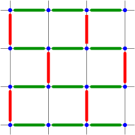
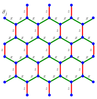
Figure 8: The brick-wall planar orbital compass model ADP (shown on the left) can be seen as a simpler relative of the XXZ honeycomb compass model, by placing it on a honeycomb lattice as shown on the right.

We provide, in the left-hand panel of Fig. 8, a simple schematic of the topology of the honeycomb lattice - that of a “brick-wall lattice”. orbital ; CN The brick-wall lattice also captures the connections in the honeycomb lattice. It is formed by the union of the highlighted vertical (red) and horizontal (green) links in the left-hand side Fig. 8. The brick-wall lattice can be obtained by “squashing” the honeycomb lattice to flatten its diagonal links while leaving its topology unchanged in the process. In the brick-wall lattice, $\hat{e}_{{\bm{l}}}$ simply becomes a unit vector along the horizontal direction. As can be seen by examining either of the panels of Fig. 8, the centers of the vertical links of the honeycomb (or brick-wall) lattice form, up to innocuous dilation factors, a square lattice. As is further evident on inspecting Fig. 8, between any pair of centers of neighboring vertical (red) links, there lies a center of a non-diagonal (green) link. This topological connection underlies the duality between the Majorana model on the square lattice and the XXZ honeycomb compass spin model. We explicitly classify the bonds in the Hamiltonian of Eq. (71) related to the two types of geometric objects:

1. Bonds of type (i) are associated with the products $\{\sigma^{x}_{{\bm{r}}}\sigma^{x}_{{\bm{r}}+\hat{e}_{{\bm{l}}}}\}$ on diagonal links of the lattice. They each anticommute with two

2. Bonds of type (ii), affiliated with products $\{\sigma^{z}_{{\bm{r}}}\sigma^{z}_{{\bm{r}}+\hat{e}_{z}}\}$ on the vertical links. Each one of these bonds anticommute with four bonds of type (i).

We merely note that replacing the bonds of the Majorana model on a square lattice, as they appear in the bond algebraic relations (1-3) of Section IV, by the ones above leads to three equivalent relations that completely specify the bond algebra of the system of Eq. (71). As we have earlier seen also the quantum Ising gauge theory of Eq. (27) and the annealed transverse-field Ising model of Eq. (48) have bonds that share the same three basic bond algebraic relations. Thus we conclude that the XXZ honeycomb compass model is exactly dual to the quantum Ising gauge theory of Eq. (27) on the square lattice. In its uniform rendition (with all couplings $J_{{\bm{l}}}$ and fields $h_{{\bm{r}}}$ being spatially uniform) the XXZ honeycomb compass system lies in the 3D Ising universality class. Similarly, many other properties of the XXZ honeycomb compass model can be inferred from the heavily investigated quantum Ising gauge theory.

The duality between the XXZ honeycomb compass model and its Majorana system equal on the square lattice affords an example of a duality in which the Hilbert space size is preserved as we now elaborate. The XXZ theory of Eq. (71) is defined on a Hilbert space of size $\dim{\cal{H}}_{\sf XXZh}=2^{N_{\sf hl}}$ where $N_{\sf hl}$ is the number of sites on the honeycomb lattice while that of the Majorana model of Eq. (5) was on a Hilbert space of dimension $\dim{\cal{H}}_{\sf M}=4^{N_{{\bm{r}}}}$. Now, for a given number $N_{{\bm{r}}}$ of vertical links on the honeycomb lattice, we have the same number of bonds of type (i) and (ii) as we had in the Majorana system while having $N_{\sf hl}=2N_{{\bm{r}}}$ lattice sites.

V.2 Checkerboard model of $(p+ip)$ superconducting grains

In Ref. XM, , Xu and Moore, motivated by an earlier work of Moore and Lee, ML proposed the following spin Hamiltonian

$$H_{\sf XM}=-\sum_{\bm{r}}(h^{\sf XM}_{{\bm{r}}}\sigma^{x}_{\bm{r}}+J_{\Box}^{\sf XM}\square\sigma^{z}_{\bm{r}})$$ (74)

to describe the time-reversal symmetry breaking characteristics in a matrix of unconventional $p$-wave granular superconductors on a square lattice. In writing Eq. (74), we employ a shorthand

$$\square\sigma^{z}_{\bm{r}}\equiv\sigma^{z}_{\bm{r}}\sigma^{z}_{{\bm{r}}+{\bm{e_{1}}}}\sigma^{z}_{{\bm{r}}+{\bm{e_{1}}}+{\bm{e_{2}}}}\sigma^{z}_{{\bm{r}}+{\bm{e_{2}}}},$$ (75)

to denote the square lattice plaquette product, where ${\bm{e_{1}}}$ and ${\bm{e_{2}}}$ denote unit vectors along the principal lattice directions. It is important to emphasize that the spins ${\bf{\sigma}}_{{\bm{r}}}^{x,z}$ in Eqs. (74), (75) are situated at the vertices ${\bm{r}}$ of the square lattice (not on the links (or link centers) as in gauge theories). The eigenvalues $\sigma^{z}_{{\bm{r}}}=\pm 1$ describe whether the superconducting grain located at the vertex of the square lattice ${\bm{r}}$ has a $(p+ip)$ or a $(p-ip)$ order parameter.

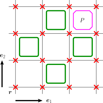
Figure 9: The checkerboard Xu-Moore (CXM) model of Eq. (76). The symmetry plaquettes $P$ constitute half of all the plaquettes of the lattice, while the interaction plaquettes $\square\sigma^{z}_{\bm{r}}$ represent the other half.

We show next that a $D=2$ checkerboard rendition of the XM model which we denote by CXM (see Fig. 9) is dual to the Majorana system on the square lattice (which is, as we showed, dual to the XXZ honeycomb compass model and all of the other models that we discussed earlier in this work). This system is defined by the following Hamiltonian

$$H_{\sf CXM}=-\sum_{\bm{r}}h_{{\bm{r}}}\sigma^{x}_{\bm{r}}-\sum_{x_{1}+x_{2}={\sf odd}}J_{\Box}^{\sf XM}\square\sigma^{z}_{\bm{r}}.$$ (76)

In this system, the plaquette operators $\square\sigma^{z}_{\bm{r}}$ (with ${\bm{r}}=x_{1}{\bm{e_{1}}}+x_{2}{\bm{e_{2}}}$) appear in every other plaquette (hence the name “checkerboard”). These plaquettes are present only if $x_{1}+x_{2}$ is an odd integer as emphasized in Eq. (76). The model has the following local symmetries

$$G_{P}=\prod_{{\bm{r}}\in P}\sigma^{x}_{\bm{r}},$$ (77)

where $P$ are those plaquettes appearing whenever $x_{1}+x_{2}$ is an even integer.

The proof of our assertion above concerning the duality of this system to the Majorana system of Eq. (5) when implemented on the square lattice is straightforward and will mirror, once again, all of our earlier steps. We may view the Hamiltonian of Eq. (76) as comprised of two basic types of bonds:

1. Bonds of type (i) are on-site operators $\{\sigma^{x}_{{\bm{r}}}\}$ associated with local transverse fields.

2. Bonds of type (ii) are the plaquette product operators $\{\square\sigma^{z}_{\bm{r}}\}$ of Eq. (75), for plaquettes whose bottom left-hand corner ${\bm{r}}$ is an “odd” site.

The basic network structure underlying these bonds is simple and, apart from an interchange of names, identical to that of the Majorana system on the square lattice of Fig. 1 as well as that of the XXZ honeycomb compass model of Fig. 8. To see this, we note that in the checkerboard of Fig. 9, the four-fold coordinated interaction plaquettes generate, on their own, a square lattice grid. Between any two neighboring interaction plaquettes on this square lattice array, there is a lattice site ${\bm{r}}$ (see Fig. 10). As in our earlier proof of the duality, we simply remark that replacing the bonds of the Majorana model on a square lattice, as they appear in the bond algebraic relations (1-3) of Section IV, by the ones above leads to three equivalent relations that completely specify the bond algebra of the CXM system. The Majorana and CXM models are thus dual to one another ($H_{\sf M}\leftrightarrow H_{\sf CXM}$) when their couplings are related via the correspondence

$$J_{{\bm{l}}}\leftrightarrow h^{\sf XM}_{{\bm{r}}},$$

$$h_{{\bm{r}}}\leftrightarrow J_{\Box}^{\sf XM}.$$ (78)

Thus, the CXM model joins the fellowship of all other dual theories (with the same network connectivity) that we discussed in this work (i.e., the Majorana, quantum Ising gauge, and annealed transverse field Ising models on the square lattice as well as the XXZ compass model on the honeycomb (or equivalent brick-wall) lattice).

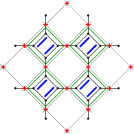
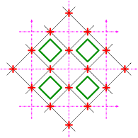
Figure 10: The $D=2$ checkerboard Xu-Moore (CXM) model is dual to the Majorana system in a square lattice as shown on the left. On the right, we rotate and redefine the lattice in a manner which highlights its connection to the quantum Ising gauge (QIG) theory of Eq. (27).

On the right-hand half of Fig. 10, we pictorially illustrate the connection between the CXM model and the quantum Ising gauge theory. The individual sites of the checkerboard lattice of Fig. 9 (the sites at which the local transverse fields are present) map onto links of the gauge theory (Section IV.1). Similarly, the interaction plaquettes of the CXM model map into plaquettes of the quantum Ising gauge theory. Note, on the right, that as is geometrically well appreciated, the four center-points of the individual links on the square (gauge theory) lattice can either circumscribe interaction plaquettes of the gauge theory or may correspond to four links that share a common endpoint that do form a “star” configuration. ADP In particular, by its duality to the quantum Ising theory, the CXM rigorously lies in the 3D Ising universality class when the couplings $J_{\Box}^{\sf XM}$ and $h^{\sf XM}_{{\bm{r}}}$ are spatially uniform. For a given equal number of bonds in both the Majorana system and the CXM theory, it is readily seen that the Hilbert space dimensions of both theories are the same, $\dim{\cal{H}}_{\sf M}=\dim{\cal{H}}_{\sf CXM}$.

VI Simulating Hubbard-like models with Majorana networks

The Dirac, fermionic, annihilation and creation operators, $\{d_{\bm{r}}\}$ and $\{d_{\bm{r}}^{\dagger}\}$ respectively, can be expressed as a linear combination of two Majorana fermion operators. For example, if we are interested in two-flavor Dirac operators a possible realization is (see Fig. 1)

$$d_{{\bm{r}}\uparrow} = \frac{1}{\sqrt{2}}(c_{{\bm{l}}_{1}1}+ic_{{\bm{l}}_{3}2}),\ d^{\dagger}_{{\bm{r}}\uparrow}=\frac{1}{\sqrt{2}}(c_{{\bm{l}}_{1}1}-ic_{{\bm{l}}_{3}2}),$$

$$d_{{\bm{r}}\downarrow} = \frac{1}{\sqrt{2}}(c_{{\bm{l}}_{2}1}+ic_{{\bm{l}}_{4}2}),\ d^{\dagger}_{{\bm{r}}\downarrow}=\frac{1}{\sqrt{2}}(c_{{\bm{l}}_{2}1}-ic_{{\bm{l}}_{4}2}),$$ (79)

where ${\bm{r}}\in{\bm{l}}_{1},{\bm{l}}_{2},{\bm{l}}_{3},{\bm{l}}_{4}$.

A system of interacting Dirac fermions (e.g., electrons) on a general graph can be mapped onto that of twice the number of Majorana fermions on the same graph, and each Dirac fermion is to be replaced by two Majorana fermions following the substitution of Eq. (VI). Thus, any granular system of the form of Eq. (5) in which each grain ${\bm{r}}$ has $q_{{\bm{r}}}=2z_{{\bm{r}}}$ neighbors, can be mapped onto a Dirac fermionic system on the same graph in which on each grain there are $z_{{\bm{r}}}$ Dirac fermions. There are many possible ways to pair up the Majorana fermions in the system of Eq. (5) to yield a corresponding system of Dirac fermions. Equation (VI) represents just one possibility. Another possible way to generate (spinless) Dirac fermions is

$$d_{\bm{l}}=\frac{1}{\sqrt{2}}(c_{{\bm{l}}1}+ic_{{\bm{l}}2}),\ d^{\dagger}_{{\bm{l}}}=\frac{1}{\sqrt{2}}(c_{{\bm{l}}1}-ic_{{\bm{l}}2}).$$ (80)

All of the spin duals that we derived for Majorana fermion systems hold, mutatis mutandis, for these systems of Dirac fermions on arbitrary graphs. In this sense, dualities afford an alternative, flexible approach to fermionization that does not rely on the Jordan-Wigner transformation. ADP Most importantly, one can use these mappings to simulate models of strongly interacting Dirac fermions, such as Hubbard-like models, on the experimentally realized Majorana networks. In other words, one can engineer quantum simulators out of these Josephson junction arrays.

As a concrete example, we consider the square-lattice array of Fig. 1 and transform, on this lattice, the Majorana system of Eq. (5) into a two-flavor Hubbard model with compass-type pairing and hopping. Based on our analysis thus far we will illustrate that this variant of the 2D Hubbard model is exactly dual to the 2D quantum Ising gauge theory and thus lies in the 3D Ising universality class. Consider the mapping of Eq. (VI). With $n_{{\bm{r}}\sigma}=d_{{\bm{r}}\sigma}^{\dagger}d_{{\bm{r}}\sigma}$ ($\sigma=\uparrow,\downarrow$), a Hubbard type term with on-site repulsion $U_{{\bm{r}}}$ becomes

$$U_{{\bm{r}}}(n_{{\bm{r}}\uparrow}-1)(n_{{\bm{r}}\downarrow}-1)=U_{{\bm{r}}}({\cal P}_{\bm{r}}-1),$$ (81)

akin to the second term of Eq. (5) with $h_{{\bm{r}}}\leftrightarrow U_{{\bm{r}}}$ (up to an irrelevant constant). In what follows we assume that the network array of Fig. 1 has unit lattice constant.

The Majorana bilinear that couples, for instance, the bottom most corner of the grain that is directly above ${\bm{r}}$ (i.e., site ${{\bm{r}}+{\bm{e_{2}}}}$) to the top-most site of grain ${\bm{r}}$ (with thus a link ${\bm{l}}$ that is vertical) becomes

$$-iJ_{{\bm{l}}}c_{{\bm{l}}_{2}1}c_{{\bm{l}}_{2}2}=\frac{J_{{\bm{l}}}}{2}(d_{{\bm{r}}\downarrow}^{\dagger}+d_{{\bm{r}}\downarrow})(d_{{\bm{r}}+{\bm{e_{2}}}\downarrow}^{\dagger}-d_{{\bm{r}}+{\bm{e_{2}}}\downarrow}).$$ (82)

Similarly, for horizontal links ${\bm{l}}$, the bilinear in the first term of Eq. (5) realizes pairing hopping terms involving only the $\uparrow$ flavor of the fermions. Thus, the Hamiltonian of Eq. (5) becomes a Hubbard type Hamiltonian with bilinear terms containing hopping and pairing terms between electrons of the up or down flavor for links ${\bm{l}}$ that are vertical or horizontal, respectively. Such a dependence of the interactions between the internal spin flavor on the relative orientation of the two interacting electrons in real-space bears a resemblance to “compass type” systems. brink Putting all our results together, the Dirac fermion Hamiltonian on the square lattice with pair terms of the form of Eq. (82) augmented by the on-site Hubbard type interaction term of Eq. (81) is dual to all of the other models that we considered thus far in this work. In particular, as such this interacting Dirac fermion (or electronic) system is not of the canonical non-interacting Fermi liquid form. Rather, this system lies in the 3D Ising universality class.

The standard Hubbard model with $SU(2)$ spin symmetry, which up to chemical potential terms is given by ($\alpha=1,2$)

$$H_{\sf Hub}=-t\sum_{{\bm{r}},\alpha,\sigma}(d_{{\bm{r}}\sigma}^{\dagger}d_{{\bm{r}}+{\bm{e}}_{\alpha}\sigma}+{\sf h.c.})$$

$$+U\sum_{{\bm{r}}}(n_{{\bm{r}}\uparrow}-1)(n_{{\bm{r}}\downarrow}-1),$$ (83)

can be written as a sum of terms of the form of Eq. (81) augmenting many Majorana Fermi bilinear coupling sites on nearest neighbor grains (i.e., ${\bm{r}}$ and ${\bm{r}}\pm{\bm{e}}_{\alpha}$). As we illustrate in Fig. 11, we label the four Majorana modes on each grain ${\bm{r}}$ as $\{c_{{\bm{r}}a}\}_{a=1}^{4}$. In terms of these, the Hubbard Hamiltonian becomes

$$H_{\sf Hub}= - t\sum_{{\bm{r}},\alpha,a=1,2}i(c_{{\bm{r}}a}c_{{\bm{r}}+{\bm{e}}_{\alpha}a+2}+c_{{\bm{r}}+{\bm{e}}_{\alpha}a}c_{{\bm{r}}a+2})$$ (84)

$$+ U\sum_{{\bm{r}}}({\cal P}_{\bm{r}}-1).$$

Thus, the Hubbard Hamiltonian may be simulated via Majorana wires with multiple Josephson junctions.

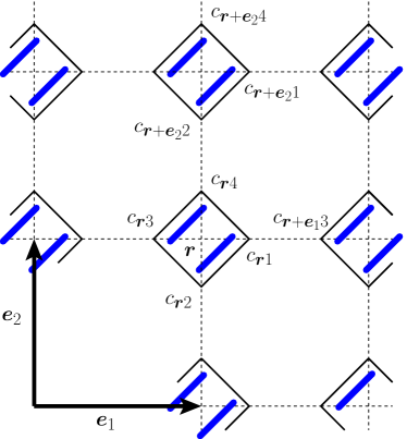
Figure 11: A labeling of the Majorana wire endpoints on the square lattice which we use here to explicitly represent the standard electronic Hubbard model in terms of Majorana operators. This is a different labeling than the one in Fig. 1.

Appendix B describes the possible simulation of quantum spin $S=1/2$ systems in terms of Majorana networks.

VII Conclusions

We conclude with a brief synopsis of our findings. This work focused on the interacting Majorana systems of Eq. (5) on general lattices and networks. By employing the standard representation of Dirac fermions as a linear combination of Majorana fermions, our results similarly hold for a general class of interacting Dirac fermion systems on general graphs. Towards this end, we heavily invoked two principal tools:

• The use of $d$-dimensional gauge-like symmetries that mandate dimensional reduction and TQO via correlation function bounds. TQO ; BN ; ads These symmetries lead to bounds on the autocorrelation times. ads

• The bond-algebraic theory of dualities ads ; NO ; bond ; orbital ; bondprl ; ADP ; clock as it, in particular, pertains to very general dualities and fermionization bondprl ; ADP to obtain multiple exact spin duals to these systems, in arbitrary dimensions and boundary conditions, and for finite or infinite systems.

Using this approach, we demonstrated that

• The Majorana systems of Eq. (5), standard quantum Ising gauge theories (Eq. (27)) and, transverse-field Ising models with annealed bimodal disorder (Eq. (48)) are all dual to one another on general lattices and networks. The duality afforded an interesting connection between heavily disordered annealed Ising systems and uniform Ising theories. The spin duals further enable us to suggest and predict various transitions as well as spin-glass type behavior in general interacting Majorana fermion (and Dirac fermion) systems. The representation of Dirac fermions via Majorana fermions enlarges the scope of our results. In particular, as Eq. (81) makes evident, the standard on-site Hubbard term in electronic systems is exactly of the same form as that of the intra-grain coupling in the interacting Majorana systems that we investigated. We similarly represented the bilinear in the Majorana model of Eq. (5) as a Dirac fermion form (Eq. (82)). Following our dualities, on the square lattice, the interacting Dirac fermion (or electronic) Hamiltonian formed by the sum of all terms of the form of Eqs. (81, 82) is dual to the quantum Ising gauge theory and thus lies in the 3D Ising universality class, notably different from standard non-interacting Fermi liquids; this non-trivial electronic system features Hubbard on-site repulsion augmented by “compass” type hopping and pairing terms. We further showed how to simulate bona fide Hubbard type electronic Hamiltonians via Majorana wire networks.

• Several new systems were introduced and investigated via the use of bond algebras:
  (1) the “XXZ honeycomb compass” model of Eq. (71) (a model intermediate between the classical Ising model on the honeycomb lattice and Kitaev’s honeycomb model and,
  (2) a checkerboard version of the Xu-Moore model for superconducting $(p+ip)$ arrays (Eq. (76)).
  By the use of dualities, we illustrated that both of these systems lie in the 3D Ising universality class.

As evident in our work, all of the considerations necessary to attain these results were, to say the least, very simple by comparison to other approaches to duality that generally require far more involved calculations. In the appendices we discuss other connections between Majorana and spin systems.

VIII Acknowledgments

This work was partially supported by NSF CMMT 1106293 at Washington University.

Appendix A Dualities in finite systems with open boundary conditions

We have, so far, studied exact dualities for the Majorana system with the Hamiltonian $H_{\sf M}$ of Eq. (5) when subject to periodic boundary conditions. We focused on periodic boundary conditions these are pertinent to the theoretical study of TQO. In this appendix, we will consider exact dualities in the presence of open boundary conditions. In doing so, we will further study finite, even quite small, square lattices. It is useful to provide a precise description of these finite dual spin systems as there is a definite possibility that this Majorana architecture may become realizable in the next few years. These dualities also allow us to illustrate the flexibility of the bond algebraic approach to dualities in handling a variety of boundary conditions exactly. As in the rest of this paper, the dualities we obtain are exact unitary equivalences. Thus, these dualities may be tested numerically by checking if the energy spectra of the two dual systems are indeed identical.

As illustrated in Section IV.1, the effective Hamiltonian $H_{\sf M}$ on the square lattice and in the bulk is dual to the $\mathds{Z}_{2}$ lattice gauge theory. In this appendix, our task is to find the boundary terms that make the duality exact in the presence of open boundary conditions. Here we only consider dualities that preserve the dimension of the Hilbert space of the two theories. We thus follow two guiding principles: 1) in the bulk, the dual spin theory remains the $\mathds{Z}_{2}$ lattice gauge theory, and 2) on the boundary, we introduce terms that preserve both the bond algebra and the dimension of the Hilbert space. Let us start with the simplest interacting case, that of two islands (grains) linked by one Josephson coupling, see Fig. 12. In this case, the Hamiltonian of Eq. (5) reads

$$H_{\sf M}=-hc_{1}c_{2}c_{3}c_{4}-h^{\prime}c_{5}c_{6}c_{7}c_{8}-Jic_{3}c_{5}.$$ (85)

This Hamiltonian acts on a Hilbert space of dimension $\dim\mathcal{H}_{\sf M}=2^{8/2}=2^{4}$. Thus, the dual theory must contain four spins and some recognizable gauge interactions. The result is

$$H_{\sf QIG}=-h\sigma^{z}_{1}-h^{\prime}\sigma^{z}_{1}\sigma^{z}_{2}\sigma^{z}_{3}\sigma^{z}_{4}-J\sigma^{x}_{1}.$$ (86)

where the single spin $\sigma^{z}_{1}$ in the Hamiltonian stands for an incomplete plaquette. One can check that the bond algebra is preserved and the two spectra are identical.

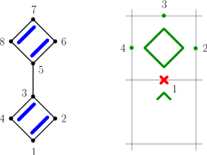
Figure 12: The spin dual of two superconducting islands. Each island maps to a plaquette interaction of the quantum Ising gauge theory, but such a mapping would not be compatible with matching dimensions of Hilbert spaces. Hence one of the lower plaquette is chopped to include only one spin.

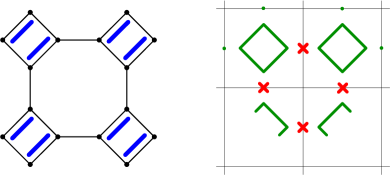
Figure 13: The spin dual for a configuration of four islands. The incomplete plaquettes represent two-spin interactions in the Hamiltonian.

The next interesting case contains four superconducting islands, see Fig. 13. In this case, $\dim\mathcal{H}_{\sf M}=2^{16/2}=2^{8}$, and so the dual spin Hamiltonian, described diagrammatically in Fig. 13 contains eight spins, two complete and two incomplete gauge plaquettes. The situation becomes more regular if we further increase the number of islands. For nine islands ($\dim\mathcal{H}_{\sf M}=2^{36/2}=2^{18}$), the Majorana system maps to eighteen spins, three complete, and six incomplete plaquettes on the first and last row of the spin model. One can generalize this picture to $L^{2}$ islands. Then the dual $\mathds{Z}_{2}$ quantum Ising gauge theory will be represented by a scaled version of the right panel of Fig. 14, with $2L^{2}$ spins, and $2L$ incomplete plaquettes (the product of only three spins $\sigma^{z}$). The latter incomplete plaquettes are equal split between the top and bottom rows, i.e., $L$ incomplete plaquettes are placed on the top row and $L$ are situated on the bottom row.

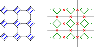
Figure 14: The spin dual for nine islands. Incomplete plaquettes represent three-spin interactions in the spin Hamiltonian, the product of the three spins $\sigma^{z}$ closer to an incomplete green diamond.

Notice that there is no natural guiding principle to find the dual theory by a Jordan-Wigner mapping. The bond-algebraic method is the natural approach and can be tested numerically on finite lattices.

Appendix B Fermionization of $S=1/2$ spin models in arbitrary dimensions

Although not pertinent to our direct models of study (those of Eq. (5) and their exact duals), we briefly review and discuss, for the sake of completeness and general perspective, dualities of related quantum spin $S=1/2$ systems. General bilinear spin Hamiltonians can be expressed as a quartic form in Majorana fermion operators. The general nature of this mapping is well known and has been applied to other spin systems with several twists. Simply put, we can write each spin operator as a quadratic form in Majorana fermions. In the case of general two-component spin systems that we discuss now, the relevant Pauli algebra is given by the following on-site $({\bm{r}}$) constraints

$$(\sigma^{x}_{{\bm{r}}})^{2}=(\sigma^{z}_{{\bm{r}}})^{2}=1,\ \{\sigma^{x}_{{\bm{r}}},\sigma^{z}_{{\bm{r}}}\}=0,$$ (87)

and trivial off-site $({\bm{r}}\neq{\bm{r}}^{\prime})$ relations,

$$[\sigma^{x}_{{\bm{r}}},\sigma^{z}_{{\bm{r}}^{\prime}}]=0.$$ (88)

A dual Majorana form may be easily derived as follows. We consider a dual Majorana system in which at each lattice site ${\bm{r}}$, there is a grain with three relevant Majorana modes. We label the three relevant Majorana modes (out of any larger number of modes on each grain) by $\{c_{{\bm{r}},a}\}_{a=1}^{3}$. As can be readily seen by invoking Eq. (4), a representation that trivially preserves the algebraic relations of Eqs. (87, 88) is given by

$$\sigma^{x}_{{\bm{r}}}\leftrightarrow ic_{{\bm{r}}1}c_{{\bm{r}}2},\ \sigma^{z}_{{\bm{r}}}\leftrightarrow ic_{{\bm{r}}1}c_{{\bm{r}}3}.$$ (89)

Equation (89) is a variant of a well known mapping applicable to three component spins (as well as, trivially, spins with any smaller number of components). Biswas ; known Equation (89) may also be viewed as a two-component version of the mapping employed by Kitaev. Kitaev06 The Hilbert space spanned by an $S=1/2$ spin system on a lattice/network having $N$ sites is $\dim{\cal{H}}_{\sf spin}=2^{N}$. By contrast, the Hilbert space of a general Majorana system with $\{m_{{\bm{r}}}\}$ Majorana modes $(m_{{\bm{r}}}\geq 3$) at sites $\{{\bm{r}}\}$ is given by $\dim{\cal{H}}_{\sf M}=2^{\sum_{{\bm{r}}}m_{{\bm{r}}}/2}$. Thus, in this duality the Hilbert space is not preserved: each individual energy level of the spin system becomes $2^{(\sum_{{\bm{r}}}m_{{\bm{r}}}/2)-N}$ fold degenerate. Similarly, one-component systems (e.g., those involving only $\{\sigma_{{\bm{r}}}^{x}\}$) can be mapped onto a granular system with two Majorana modes per site. If there are two Majorana modes at each site ${\bm{r}}$ then such a mapping will preserve the Hilbert space size.

For completeness, we now turn to specific spin systems related to those that we discussed in the main part of our article. In Section V.2, we illustrated that the Majorana system of Eq. (5) (and all of its duals that we earlier discussed in the text) can be mapped onto the Xu-Moore model XM on the checkerboard lattice. Following our general discussion above, it is straightforward to provide a Majorana dual to the Xu-Moore model on the square lattice, Eq. (74). On the square lattice, the orbital compass model (OCM) and the Xu-Moore model of Eq. (74) are dual to one another. bondprl ; ADP ; NF We will assume the square lattice to define the $xz$ plane. The anisotropic square lattice OCM NF ; brink is given by the Hamiltonian

$$H_{\sf OCM}=-\sum_{{\bm{r}}}(J_{x;{\bm{r}}}\sigma^{x}_{{\bm{r}}}\sigma^{x}_{{\bm{r}}+{\bm{e_{1}}}}+J_{z;{\bm{r}}}\sigma^{z}_{{\bm{r}}}\sigma^{z}_{{\bm{r}}+{\bm{e_{2}}}}).$$ (90)

In Eq. (90), we generalized the usual compass model Hamiltonian by allowing the couplings $\{J_{x,z}\}$ to vary locally with the location of the horizontal and vertical links of the square lattice (given by $({\bm{r}},{\bm{r}}+{\bm{e}}_{1,2})$ respectively). By plugging Eq. (89) into Eq. (90), we can rewrite this (as well as other general two-component spin bilinears) as a quartic form in the Majorana fermions.

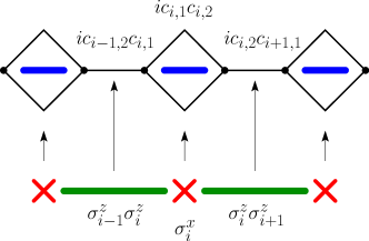
Figure 15: The transverse-field Ising model can be simulated by an architecture of nanowires with one wire per superconducting island.

It may generally be feasible to use our formalism to simulate quantum spin models in terms of Majorana networks. Consider, for example, the simulation of a transverse-field Ising chain

$$H_{\sf I}=-\sum_{i=1}^{N-1}J_{i}\sigma^{z}_{i}\sigma^{z}_{{i+1}}-\sum_{i=1}^{N}h_{i}\sigma^{x}_{i}.$$ (91)

with $N$ spins and open boundary conditions. In this case, it may be possible to use linear arrays with one nanowire per island to simulate this model and study, for instance, the dynamics of its quantum phase transition. The Hamiltonian $H_{\sf I}$ maps to the Majorana network

$$H_{\sf M}=-i\sum_{i=1}^{N-1}J_{i}c_{i,2}c_{i+1,1}-i\sum_{i=1}^{N}h_{i}c_{i,1}c_{i,2},$$ (92)

after the following duality mapping

$$\sigma^{z}_{i}\sigma^{z}_{i+1}\mapsto ic_{i,2}c_{i+1,1}\ ,\ \sigma^{x}_{i}\mapsto ic_{i,1}c_{i,2},$$ (93)

see Fig. 15.

References

- (1) E. Majorana, Nuovo Cimento 14, 171 (1937).
- (2) C. W. J. Beenakker, arXiv:1112.1950 (2011).
- (3) F. Wilczek, Nature Physics 5, 614 (2009).
- (4) M. Franz, Physics 3, 24 (2010).
- (5) J. Alicea, Phys. Rev. B 81, 125318 (2010).
- (6) L. Fu and C. L. Kane, Phys. Rev. Lett. 100, 096407 (2008).
- (7) J. Nilsson, A. R. Akhmerov, and C. W. Beenakker, Phys. Rev. Lett. 101, 120403 (2008).
- (8) A. Yu. Kitaev, Phys.-Usp. 44 (supplement), 131 (2001).
- (9) J. D. Sau, R. M. Lutchyn, S. Tewari, and S. Das Sarma, Phys. Rev. Lett. 104, 040502 (2010).
- (10) Y. Oreg, G. Refael, and F. von Oppen, Phys. Rev. Lett. 105, 177002 (2010).
- (11) R. R. Biswas, C. R. Laumann, and S. Sachdev, Phys. Rev. B 84, 235148 (2011).
- (12) H-H. Lai and O. I. Motrunich, Phys. Rev. B 84, 235148 (2011).
- (13) D. Ivanov, Phys. Rev. Lett. 86, 268 (2001).
- (14) N. Read and D. Green, Phys. Rev. B 61, 10267 (2000).
- (15) S. Deng, L. Viola, and G. Ortiz, Phys. Rev. Lett. 108, 036803 (2012).
- (16) L. Fu, Phys. Rev. Lett. 104, 056402 (2010)
- (17) A. Kitaev, Ann. of Phys. 321, 2 (2006).
- (18) C. Xu and L. Fu, Phys. Rev. B 81, 134435 (2010).
- (19) B. M. Terhal, F. Hassler, and D. P. DiVincenzo, arXiv:1201.3757.
- (20) A. Kitaev, Ann. of Phys. 303, 2 (2003).
- (21) C. Nayak, C. Simon, C. A. Stern, M. Freedman, and S. Das Sarma, Rev. Mod. Phys. 80, 1083 (2008).
- (22) E. Lieb, T. Schultz, and D. Mattis, Ann. of Phys. 16, 407 (1961).
- (23) S. Nadj-Perge, V. S. Pribiag, J. W. G. van den Berg, K. Zuo, S. R. Plissard, E. P. A. M. Bakkers, S. M. Frolov, and L. P. Kouwenhoven, arXiv:1201.3707v1.
- (24) Z. Nussinov and G. Ortiz, Ann. of Phys. 324, 977 (2009); Z. Nussinov and G. Ortiz, PNAS 106, 16944 (2009).
- (25) C. D. Batista and Z. Nussinov, Phys. Rev. B 72, 045137 (2005).
- (26) Z. Nussinov, G. Ortiz, and E. Cobanera, arXiv:1110.2179.
- (27) E. Fradkin, M. Srednicki, and L. Susskind, Phys. Rev. D 21, 2885 (1979).
- (28) Z. Nussinov and G. Ortiz, Phys. Rev. B 77, 064302 (2008).
- (29) Z. Nussinov and G. Ortiz, Phys. Rev. B 79, 214440 (2009).
- (30) Z. Nussinov and G. Ortiz, Europhysics Letters 84, 36005 (2008).
- (31) E. Cobanera, G. Ortiz, and Z. Nussinov, Phys. Rev. Lett. 104, 20402 (2010).
- (32) E. Cobanera, G. Ortiz, and Z. Nussinov, Adv. in Phys. 60, 679 (2011).
- (33) G. Ortiz, E. Cobanera, and Z. Nussinov, Nucl. Phys. B 854, 780 (2011).
- (34) On each grain, the non-intersecting nanowires link one half of the nanowire endpoints to the remaining half; there are distinct ways for different pairings of the vertices. These non-intersecting nanowires can be placed in any way on a surface of the bulk superconducting grain. For instance, in the square and triangular lattices, the regular arrangement of nanowires shown in Figs. 1, and 3 is only one among many others.
-
(35)
It us useful at this point to recall some basic algebraic facts about
Majorana fermions. Let us label the Majorana operators simply
as . Then,
In general,(94)
so that the eigenvalues of are or , depending on . If is even, up to equivalence, there is only one irreducible representation (irrep) for these relations. It acts on a Hilbert space of dimension , and can be described in terms of Pauli matrices as(95)
If is odd,(96)
So in view of Eq. (95), the irreps of Eq. (94) are characterized by an extra constraint,(97)
with depending on and the particular irrep. An explicit irrep is afforded by(98)
Its dimension is .(99) (103) - (36) A definite order is to be assigned on each grain. As will become evident, an odd permutation of the ordering of the Majorana operators in the product of Eq. (6), which leads by virtue of the Majorana algebra to a sign change, will not change the bond algebra (to be defined later) and thus none of our dualities.
-
(37)
In these and other general systems, not all gauge-like
symmetries are independent. If the Majorana system has a trivial
homology (such as that of an infinite plane or a sphere), no
gauge-like symmetries appear: all symmetries involving
sites can be expressed in terms of a product of the local symmetries
and thus are not fundamental. By contrast, for a dimensional
system placed on a torus there are two closed toric cycles
independent of the local symmetries. This explains the findings of Ref.
Terhal, that the Majorana theory has TQO. Some
manifestations of this phenomenon were noticed in numerical simulations
of compact QED jersak , though not recognized as a signal of the
presence or absence of TQO. In numerous theories with plaquette and/or
link interactions, the Euler-Lhuillier formula
relating the genus number of the manifold on which the system is embedded to the number of local faces (), edges (), and vertices () affords us with a knowledge of the number of independent () symmetry operators (loops around independent cycles) that the system may have that cannot be written in terms of local operators. This and related aspects have been discussed elsewhere TQO .(104) - (38) E. Fradkin and L. Susskind, Phys. Rev. D 17, 2637 (1978).
- (39) S. Elitzur, Phys. Rev. D 12, 3978 (1975).
- (40) R. L. Jack and L. Berthier, Phys. Rev. E 85, 021120 (2012).
- (41) F. J. Wegner, J. of Math. Phys. 12, 2259 (1971).
- (42) J. B. Kogut, Rev. Mod. Phys. 51, 659 (1979).
- (43) N. Lacevic, F. W. Starr, T. B. Schroder, and S. C. Glotzer, J. Chem. Phys. 119, 7372 (2003).
- (44) C. Itzykson and K-M. Drouffe, Statistical Field Theory (Cambridge University Press, Cambridge, 1989), see Volume 1 (page 355, in particular).
- (45) R. B. Griffiths, Phys. Rev. Lett. 23, 17 (1969).
- (46) D. S. Fisher, Phys. Rev. Lett. 69, 534 (1992).
- (47) M. Schechter, Phys. Rev. B 77, 020401 (R) (2008).
- (48) L. B. Ioffe and M. Mezard, Phys. Rev. Lett. 105, 037001 (2010); M. V. Feigelman, L. B. Ioffe, and M. Mezard, Phys. Rev. B 82, 184534 (2010).
- (49) M. B. Salamon and M. Jaime, Rev. Mod. Phys. 73, 583 (2001); B. Kalisky, J. R. Kirtley, J. G. Analytis, J.-H. Chu, A. Vailionis, I. R. Fisher, and K. A. Moler, Phys. Rev. B 81, 184513 (2010); J. R. Kirtley, B. Kalisky, L. Luan, and K. A. Moler, Phys. Rev. B 81, 184514 (2010); J. M. Tranquada, B. J. Sternlieb, J. D. Axe, Y. Nakamura, and S. Uchida, Nature 375, 561 (1995); K. Yamada, C. H. Lee, K. Kurahashi, J. Wada, S. Wakimoto, S. Ueki, H. Kimura, Y. Endoh, S. Hosoya, G. Shirane, et al., Phys. Rev. B 57, 6165 (1998); S. R. White and D. J. Scalapino, Phys. Rev. Lett. 80, 1272 (1998); J. Zaanen and O. Gunnarsson, Phys. Rev. B 40, 7391 (1989); Kazushige and Machida, Physica C: Superconductivity 158, 192 (1989); V. Emery and S. Kivelson, Physica C: Superconductivity 209, 597 (1993); A. A. Koulakov, M. M. Fogler, and B. I. Shklovskii, Phys. Rev. Lett. 76, 499 (1996); M. P. Lilly, K. B. Cooper, J. P. Eisenstein, L. N. Pfeiffer, and K. W. West, Phys. Rev. Lett. 82, 394 (1999); R. Du, D. Tsui, H. Stormer, L. Pfeiffer, K. Baldwin, and K. West, Solid State Communications 109, 389 (1999).
- (50) S. Bogdanovich and D. Popovic, Phys. Rev. Lett. 88, 236401 (2002); J. Jaroszynski, D. Popovic, and T. M. Klapwijk, Phys. Rev. Lett. 89, 276401 (2002); J. Jaroszynski, D. Popovic, and T. M. Klapwijk, Phys. Rev. Lett. 92, 226403 (2004) V. Orlyanchik and Z. Ovadyahu 92, 066801 (2004); M. Pollak and Z. Ovadyahu, Phys. Stat. Sol. (c) 2, 283 (2006). A. Vaknin, Z. Ovadyahu, and M. Pollak, Phys. Rev. Lett. 84, 3402 (2000); Z. Ovadyahu, Phys. Rev. B 73, 214208 (2006).
- (51) C. Xu and J. E. Moore, Nucl. Phys. B 716, 487 (2005); C. Xu and J. E. Moore, Phys. Rev. Lett. 93, 047003 (2004).
- (52) J. E. Moore and D-H. Lee, Phys. Rev. B 69, 104511 (2004).
- (53) H-D. Chen and Z. Nussinov, J. of Phys. A 41, 075001 (2008).
- (54) J. L. Martin, Proc. Roy. Soc. A 251, 536 (1959); A. M. Tsvelik, Phys. Rev. Lett. 69, 2142 (1992); P. Coleman, E. Miranda, and A. Tsvelik, Phys. Rev. Lett. 70, 2960 (1993); B. Sriram Shastry and Diptiman Sen, Phys. Rev. B, 55, 2988 (1997); F. Wang and A. Vishwanath, Phys. Rev. B 80, 064413 (2009).
- (55) J. van den Brink, New J. Phys. 6, 201 (2004).
- (56) Z. Nussinov and E. Fradkin, Phys. Rev. B 71, 195120 (2005).
- (57) J. Jersak et. al., Phys. Rev. Lett. 77, 1933 (1996).