Noncommutative Hodge-to-de Rham spectral sequence and the Heegaard Floer homology of double covers

Abstract.

Let $A$ be a dg algebra over ${\mathbb{F}_{2}}$ and let $M$ be a dg $A$-bimodule. We show that under certain technical hypotheses on $A$, a noncommutative analog of the Hodge-to-de Rham spectral sequence starts at the Hochschild homology of the derived tensor product $M\otimes^{L}_{A}M$ and converges to the Hochschild homology of $M$. We apply this result to bordered Heegaard Floer theory, giving spectral sequences associated to Heegaard Floer homology groups of certain branched and unbranched double covers.

1. Introduction

This paper is inspired by a theorem of Hendricks and a question of Lidman. In turn, they are:

Theorem 1.1.

[Hen12, Theorem 1.1] Let $K\subset S^{3}$ be a knot and $\pi\nobreak\mskip 2.0mu\mathpunct{}\nonscript\mkern-3.0mu{:}\penalty 300\mskip 6.0mu plus 1.0mu\Sigma(K)\to S^{3}$ the double cover of $S^{3}$ branched along $K$. For $n$ sufficiently large there is a spectral sequence with $E^{1}$-page given by the knot Floer homology group $\widehat{\mathit{HFK}}(\Sigma(K),\pi^{-1}(K))\otimes H_{*}(T^{n})$ converging to $\widehat{\mathit{HFK}}(S^{3},K)\otimes H_{*}(T^{n})$.

(Here, $\widehat{\mathit{HFK}}(Y,K)$ denotes the knot Floer homology group of $(Y,K)$ [OSz04, Ras03] with coefficients in ${\mathbb{F}_{2}}$, and $H_{*}(T^{n})$ denotes the singular homology of the $n$-torus.)

Hendricks deduces Theorem 1.1 from Seidel-Smith’s localization theorem for Lagrangian intersection Floer homology [SS10]. In particular, the proof is basically analytic. Lidman asked:

Question 1.

(Lidman) Is it possible to recover Theorem 1.1 from cut-and-paste arguments?

In this paper we give a partial affirmative answer to Question 1; moreover, our techniques can be used in situations where the hypotheses of Seidel-Smith’s theorem fail. The idea is as follows. Bordered Floer homology allows one to interpret the knot Floer homology of $K$ as the Hochschild homology of a bimodule [LOT10, Theorem 14]. In characteristic 2 we show that there is a spectral sequence which under certain technical hypotheses (see Theorem 4) has the form

(1.2) $$\mathit{HH}_{*}(M\otimes^{L}_{A}M)\Rightarrow\mathit{HH}_{*}(M),.$$

where $M\otimes^{L}_{A}M$ denotes the derived tensor product (over $A$) of $M$ with itself. If the technical hypotheses are satisfied for the algebras in bordered Floer theory, the spectral sequence (1.2) gives another proof of Theorem 1.1, as well as many generalizations.

The technical hypotheses needed for (1.2) in the case of bordered Floer homology boil down to a fairly concrete, combinatorial problem. We have not been able to solve this problem in general, but do give two partial results along these lines. Thus, we obtain localization results for Heegaard Floer and knot Floer homology groups, different from but overlapping with Theorem 1.1:

Theorem 1.

Let $Y^{3}$ be a closed $3$-manifold, $K\subset Y$ a nullhomologous knot and $\mathfrak{s}$ a torsion $\operatorname{spin}^{c}$-structure on $Y\setminus K$. Suppose that $K$ has a genus $2$ Seifert surface $F$. Then for each Alexander grading $i$ there is a spectral sequence

$$\widehat{\mathit{HFK}}(\Sigma(K),\pi^{-1}(K);\pi^{*}\mathfrak{t},i)\Rightarrow\widehat{\mathit{HFK}}(Y,K;\mathfrak{t},i).$$

(This is proved in Section 4.3. A simplified statement in the special case of knots in $S^{3}$ is given as Corollary 10.)

Theorem 2.

Let $Y^{3}$ be a closed $3$-manifold, $K\subset Y$ a nullhomologous knot and $\mathfrak{s}$ a torsion $\operatorname{spin}^{c}$-structure on $Y\setminus K$. Let $F$ be a Seifert surface for $K$, of some genus $k$. Then there is a spectral sequence

$$\widehat{\mathit{HFK}}(\Sigma(K),\pi^{-1}(K);\pi^{*}\mathfrak{t},k-1)\Rightarrow\widehat{\mathit{HFK}}(Y,K;\mathfrak{t},k-1).$$

(Again, this is proved in Section 4.3.)

Our techniques also apply to certain unbranched double covers. Specifically, let $Y$ be a closed $3$-manifold and $\pi\nobreak\mskip 2.0mu\mathpunct{}\nonscript\mkern-3.0mu{:}\penalty 300\mskip 6.0mu plus 1.0mu\tilde{Y}\to Y$ a $\mathbb{Z}/2$-cover. Viewing $\pi$ as an element of $H^{1}(Y;{\mathbb{F}_{2}})$, assume $\pi$ is in the image of $H^{1}(Y;\mathbb{Z})$. In this case we say that $\pi$ is induced by a $\mathbb{Z}$-cover (Definition 4.33).

Theorem 3.

Let $Y$ be a closed $3$-manifold and $\pi\nobreak\mskip 2.0mu\mathpunct{}\nonscript\mkern-3.0mu{:}\penalty 300\mskip 6.0mu plus 1.0mu\tilde{Y}\to Y$ a $\mathbb{Z}/2$-cover which is induced by a $\mathbb{Z}$-cover. Let $\mathfrak{s}\in\operatorname{spin}^{c}(Y)$ be a torsion $\operatorname{spin}^{c}$-structure. Then there is a spectral sequence

$$\widehat{\mathit{HF}}(\tilde{Y};\pi^{*}\mathfrak{s})\otimes H_{*}(S^{1})\Rightarrow\widehat{\mathit{HF}}(Y;\mathfrak{s}).$$

(This is proved in Section 4.5.)

Theorems 1 and 2 for knots in $S^{3}$ are, modulo the $H_{*}(T^{n})$ factors and decomposition according to Alexander gradings, special cases of Hendricks’s Theorem 1.1. Theorems 1 and 2 for knots in other $3$-manifolds, as well as Theorem 3, seem not to be accessible via Hendricks’s techniques. Specifically, a Chern class computation shows that the stable normal triviality condition required by Seidel-Smith always fails in these cases; see [Hen12, Remark 7.1].

The spectral sequence (1.2) is closely related to the noncommutative Hodge-to-de Rham spectral sequence (i.e. the Hochschild-to-cyclic spectral sequence). For instance, when $A$ is Calabi-Yau, we show that the technical condition on $A$ giving (1.2) is satisfied whenever the Hodge-to-de Rham spectral sequence degenerates. Also recall that the Hodge-to-de Rham spectral sequence comes by analyzing an action of $\mathrm{U}(1)$ on the Hochschild chain complex of $A$. The full rotation group does not act on the Hochschild chain complex of a bimodule, but the subgroup $\mathbb{Z}/2\subset\mathrm{U}(1)$ does act on the Hochschild chain complex of the tensor square of a bimodule. The spectral sequence (1.2) comes by analyzing this action.

Remark 1.3.

There is another resemblance between the algebra in this paper and the noncommutative Hodge-to-de Rham spectral sequence, about which we understand less. Whether or not our technical condition (“$\pi$-formality”) holds, we construct a spectral sequence starting at $\mathit{HH}_{*}(M\otimes^{L}_{A}M)$, but we cannot always identify its $E_{\infty}$-page. When $M$ is $\pi$-formal, the identification $\mathit{HH}_{*}(M)\stackrel{{\scriptstyle\sim}}{{\to}}E_{\infty}$ is a kind of squaring map, but this map is not well-defined at the level of Hochschild chains. There is (as has been pointed out to us independently by Yan Soibelman, Tyler Lawson, and the referee), a similar phenomenon at the heart of Kaledin’s work [Kal09] on the degeneration of the Hodge-to-de Rham spectral sequence: a squaring or more general Frobenius map defined on Hochschild homology of algebras (with values in a form of cyclic homology) that is not induced by a map of chain complexes. An explanation in terms of stable homotopy is given in [Kal08] — it would be interesting to see if this explanation applies in our setup as well.

Beyond bordered Floer homology, there are a number of other cases in which one could try to apply the spectral sequence (1.2) (i.e., Theorem 4). One obvious class of examples is provided by Khovanov and Khovanov-Rozansky knot homologies. Another comes from Fukaya categories. Let $(M,\omega)$ be a symplectic manifold and $\phi\nobreak\mskip 2.0mu\mathpunct{}\nonscript\mkern-3.0mu{:}\penalty 300\mskip 6.0mu plus 1.0muM\to M$ a symplectomorphism. Then $\phi$ induces an automorphism $\phi_{*}$ of the Fukaya category $\operatorname{Fuk}(M)$ of $M$. According to the philosophy of [Kon95, Sei09], if $M$ contains enough Lagrangians then $\operatorname{Fuk}(M)$ controls the Floer theory of $M$. A special case of this is the following well-known folk conjecture:

Conjecture 1.4.

Let $(M,\omega)$ be a symplectic manifold for which the Fukaya category $\operatorname{Fuk}(M)$ of $M$ and the quantum cohomology $\mathit{QH}^{*}(M)$ of $M$ are defined over ${\mathbb{F}_{2}}$. Suppose further that the natural map $\mathit{HH}_{*}(\operatorname{Fuk}(M))\to\mathit{QH}^{*}(M)$ is an isomorphism. Let $\phi\nobreak\mskip 2.0mu\mathpunct{}\nonscript\mkern-3.0mu{:}\penalty 300\mskip 6.0mu plus 1.0muM\to M$ be a symplectomorphism with fixed-point Floer homology $\mathit{HF}(\phi)$. Then

(1.5) $$\mathit{HF}(\phi)\cong\mathit{HH}_{*}\bigl{(}\phi_{*}\nobreak\mskip 2.0mu\mathpunct{}\nonscript\mkern-3.0mu{:}\penalty 300\mskip 6.0mu plus 1.0mu\operatorname{Fuk}(M)\to\operatorname{Fuk}(M)\bigr{)}.$$

Thus, for $M$ as in the statement of Conjecture 1.4, when $\operatorname{Fuk}(M)$ satisfies (appropriate analogues of) the technical hypotheses of Theorem 4, the spectral sequence (1.2) implies that

(1.6) $$\dim\mathit{HF}(\phi^{2})\geq\dim\mathit{HF}(\phi).$$

This inequality has nontrivial consequences. For example, for $\tau$ the hyperelliptic involution of a genus $g$ surface, it is easy to see that $\mathit{HF}(\tau)$ has dimension $2g+2$: the $2g+2$ fixed points of $\tau$ lie in different Nielsen classes. Formula (1.6) then implies that any (non-degenerate) map Hamiltonian-isotopic to $\tau^{2}=\mathbb{I}$ has at least $2g+2$ fixed points, a statement which does not hold for arbitrary smooth maps in the isotopy class. (Of course, this result also follows from the Arnold conjecture.)

In the special case of area-preserving diffeomorphisms of a surface with boundary $S^{1}$, it should be possible to combine Theorem 2 with the isomorphisms between Heegaard Floer homology, embedded contact homology, Seiberg-Witten Floer homology and periodic Floer homology [Tau10a, Tau10b, Tau10c, Tau10d, Tau10e, LT12, KLT10a, KLT10b, KLT10c, KLT11, KLT12, CGH12b, CGH12c, CGH12a] to obtain the inequality (1.6) without using Conjecture 1.4.

This paper is organized as follows. Section 2 gives a brief review of $\mathbb{Z}/2$-localization for singular homology; this is not needed for what follows, but should help elucidate the structure of later arguments. Section 3 is the algebraic part of the paper. We start with a review of Hochschild homology (Section 3.1) and a short review of spectral sequences associated to bicomplexes (Section 3.2), partly to fix notation. We then explain the basic algebraic condition, which we call $\pi$-formality, under which the spectral sequence (1.2) holds (Section 3.3). We then discuss when this condition holds for all $A$-bimodules; this is $\pi$-formality of $A$ (Section 3.4). For Theorems 1 and 2, this is all the algebra we need. For Theorem 3 we need one more notion, that of neutral bimodules, bimodules on which the Serre functor acts trivially in a certain sense (Section 3.5). (If $A$ is Calabi-Yau then every bimodule is neutral.) The last two subsections of Section 3 do not (yet) have topological applications, but are included to help set $\pi$-formality in a broader context. Specifically, in Section 3.6 we discuss the case that $A$ admits an integral lift; in this case, $\pi$-formality is (in some sense) easier to verify. In Section 3.7 we show that if $A$ is Calabi-Yau then the condition of $\pi$-formality follows from collapse of the Hodge-to-de Rham spectral sequence.

Section 4 is devoted to applications of the algebraic results to Heegaard Floer homology. It starts by collecting background on bordered and bordered-sutured Heegaard Floer homology (Section 4.1); there, we also observe homological smoothness for the relevant algebras. We discuss $\pi$-formality of the bordered and bordered-sutured algebras (Section 4.2). While $\pi$-formality in general remains a conjecture, we verify this conjecture in several interesting cases. The first application is to branched double covers of links, giving Theorems 1 and 2 (Section 4.3). We then discuss a particular bordered-sutured $3$-manifold, the so-called tube-cutting piece (Section 4.4) and, using this manifold, obtain a localization result for ordinary double covers, Theorem 3 (Section 4.5).

Acknowledgments

We thank Mohammed Abouzaid, Tyler Lawson, Dan Lee, Ciprian Manolescu, Junecue Suh and Yan Soibelman for helpful discussions. We especially thank Tye Lidman for suggesting that bordered Floer homology might be used to study covering spaces and for many corrections to a draft of this paper, and Kristen Hendricks for her work inspiring these results and for many helpful conversations. Finally, we thank the referee for a careful reading and many helpful and interesting comments.

The ideas in Section 4.4 arose in discussions of Peter Ozsváth, Dylan Thurston and the first author, and were observed independently by Rumen Zarev.

2. Review of $\mathbb{Z}/2$-localization for singular homology

To ease into the algebra, we start by reviewing a particular perspective on the localization theorem for $\mathbb{Z}/2$-equivariant singular homology.

Consider a topological space $X$ with a $\mathbb{Z}/2$-action $\tau\nobreak\mskip 2.0mu\mathpunct{}\nonscript\mkern-3.0mu{:}\penalty 300\mskip 6.0mu plus 1.0muX\to X$. The (Borel) equivariant cohomology of $X$ is defined to be the singular cohomology

(2.1) $$H^{*}_{\mathbb{Z}/2}(X;\mathbb{Z})\coloneqq H^{*}(X\times_{\mathbb{Z}/2}E\mathbb{Z}/2;\mathbb{Z}),$$

where $E\mathbb{Z}/2$ is a contractible space with a free $\mathbb{Z}/2$-action (e.g., $E\mathbb{Z}/2=S^{\infty}$).

Equivalently, the $\mathbb{Z}/2$-action on $X$ induces a $\mathbb{Z}/2$-action on the singular chains $C_{*}(X)$, i.e., makes $C_{*}(X)$ into a chain complex over the group ring $\mathbb{Z}[\mathbb{Z}/2]$. So, we could define

(2.2) $$H^{*}_{\mathbb{Z}/2}(X;\mathbb{Z})\coloneqq\operatorname{Ext}_{\mathbb{Z}[\mathbb{Z}/2]}(C_{*}(X),\mathbb{Z}),$$

where $\mathbb{Z}$ is given the trivial $\mathbb{Z}/2$-action. Since $C_{*}(X\times E\mathbb{Z}/2)$ is a free resolution of $C_{*}(X)$ as a $\mathbb{Z}[\mathbb{Z}/2]$-module, Equations (2.1) and (2.2) are equivalent. One advantage of Equation (2.2) is that it allows one to define an equivariant homology for any chain complex over $\mathbb{Z}[\mathbb{Z}/2]$. Another advantage is that it allows one to use other models for $C_{*}(X)$, like the cellular chain complex for $X$ (if $X$ was a CW complex and the $\mathbb{Z}/2$-action was cellular).

A particularly nice projective resolution of $\mathbb{Z}$ as a $\mathbb{Z}[\mathbb{Z}/2]$-module is given by

$$0\longleftarrow\mathbb{Z}[\mathbb{Z}/2]\stackrel{{\scriptstyle 1-\tau}}{{\longleftarrow}}\mathbb{Z}[\mathbb{Z}/2]\stackrel{{\scriptstyle 1+\tau}}{{\longleftarrow}}\mathbb{Z}[\mathbb{Z}/2]\stackrel{{\scriptstyle 1-\tau}}{{\longleftarrow}}\mathbb{Z}[\mathbb{Z}/2]\stackrel{{\scriptstyle 1+\tau}}{{\longleftarrow}}\cdots.$$

(This resolution comes from thinking of the cellular chain complex for the usual $\mathbb{Z}/2$-equivariant cell structure on $S^{\infty}$, say.) Tensoring over $\mathbb{Z}$ with $C_{*}(X)$ gives a projective resolution of $C_{*}(X)$ over $\mathbb{Z}[\mathbb{Z}/2]$

(2.3) $$0\longleftarrow C_{*}(X;\mathbb{Z})\otimes\mathbb{Z}[\mathbb{Z}/2]\stackrel{{\scriptstyle 1\otimes 1-1\otimes\tau}}{{\longleftarrow}}C_{*}(X;\mathbb{Z})\otimes\mathbb{Z}[\mathbb{Z}/2]\stackrel{{\scriptstyle 1\otimes 1+1\otimes\tau}}{{\longleftarrow}}C_{*}(X;\mathbb{Z})\otimes\mathbb{Z}[\mathbb{Z}/2]\stackrel{{\scriptstyle 1\otimes 1-1\otimes\tau}}{{\longleftarrow}}\cdots$$

where $\mathbb{Z}/2$ acts diagonally on each term. So, $H^{*}_{\mathbb{Z}/2}(X;\mathbb{Z})$ is the homology of the total complex associated to the bicomplex

(2.4) $$C^{*}_{\mathrm{Borel}}(X;\mathbb{Z})\coloneqq\bigl{(}0\longrightarrow C^{*}(X;\mathbb{Z})\stackrel{{\scriptstyle 1-\tau^{*}}}{{\longrightarrow}}C^{*}(X;\mathbb{Z})\stackrel{{\scriptstyle 1+\tau^{*}}}{{\longrightarrow}}C^{*}(X;\mathbb{Z})\stackrel{{\scriptstyle 1-\tau^{*}}}{{\longrightarrow}}C^{*}(X;\mathbb{Z})\stackrel{{\scriptstyle 1+\tau^{*}}}{{\longrightarrow}}\cdots\bigr{)}$$

obtained from Formula (2.3) by taking $\operatorname{Hom}$ over $\mathbb{Z}[\mathbb{Z}/2]$ to $\mathbb{Z}$.

The projection map $X\times_{\mathbb{Z}/2}E\mathbb{Z}/2\to(E\mathbb{Z}/2)/(\mathbb{Z}/2)\eqqcolon B\mathbb{Z}/2\simeq\mathbb{R}P^{\infty}$ endows $H^{*}_{\mathbb{Z}/2}(X;\mathbb{Z})$ with an action of $H^{*}(\mathbb{R}P^{\infty};\mathbb{Z})$. Let $\theta\in H^{2}(\mathbb{R}P^{\infty})\cong\mathbb{Z}/2$ be a generator. Multiplication by $\theta$ annihilates $p^{n}$ torsion for any $p\neq 2$, so it is natural to consider equivariant cohomology with ${\mathbb{F}_{2}}$-coefficients. Over ${\mathbb{F}_{2}}$, $H^{*}(\mathbb{R}P^{\infty};{\mathbb{F}_{2}})\cong{\mathbb{F}_{2}}[\eta]$, where $\eta\in H^{1}(\mathbb{R}P^{\infty};{\mathbb{F}_{2}})$, and the localization theorem states that under appropriate hypotheses,

(2.5) $$\eta^{-1}H^{*}_{\mathbb{Z}/2}(X;{\mathbb{F}_{2}})\coloneqq H^{*}_{\mathbb{Z}/2}(X;{\mathbb{F}_{2}})\otimes_{H^{*}(B\mathbb{Z}/2;{\mathbb{F}_{2}})}{\mathbb{F}_{2}}[\eta,\eta^{-1}]\cong H^{*}(X^{\mathrm{fix}};{\mathbb{F}_{2}})\otimes_{\mathbb{F}_{2}}{\mathbb{F}_{2}}[\eta,\eta^{-1}],$$

where $X^{\mathrm{fix}}$ denotes the fixed set of $\tau$.

Inverting $\eta$ before taking cohomology allows us to give a chain-level statement of the localization theorem. That is, consider the Tate complex of $(X,\tau)$

$$C^{*}_{\mathrm{Tate}}(X;{\mathbb{F}_{2}})\coloneqq\bigl{(}\cdots\stackrel{{\scriptstyle 1+\tau}}{{\longrightarrow}}C^{*}(X;{\mathbb{F}_{2}})\stackrel{{\scriptstyle 1+\tau}}{{\longrightarrow}}C^{*}(X;{\mathbb{F}_{2}})\stackrel{{\scriptstyle 1+\tau}}{{\longrightarrow}}C^{*}(X;{\mathbb{F}_{2}})\stackrel{{\scriptstyle 1+\tau}}{{\longrightarrow}}C^{*}(X;{\mathbb{F}_{2}})\stackrel{{\scriptstyle 1+\tau}}{{\longrightarrow}}\cdots\bigr{)},$$

a periodic analogue of $C^{*}_{\mathrm{Borel}}$. The localization theorem is then the statement that the Tate equivariant cohomology satisfies $H^{*}_{\mathrm{Tate}}(X;{\mathbb{F}_{2}})\coloneqq h_{*}(C^{*}_{\mathrm{Tate}}(X;{\mathbb{F}_{2}}))\cong H^{*}(X^{\mathrm{fix}};{\mathbb{F}_{2}})\otimes_{\mathbb{F}_{2}}{\mathbb{F}_{2}}[\eta,\eta^{-1}]$.

In the paper, we will actually work with $\mathbb{Z}/2$-equivariant homology, i.e.,

$$H_{*}^{\mathbb{Z}/2}(X;{\mathbb{F}_{2}})=H_{*}(X\times_{\mathbb{Z}/2}E\mathbb{Z}/2;{\mathbb{F}_{2}})=\operatorname{Tor}_{{\mathbb{F}_{2}}[\mathbb{Z}/2]}(C_{*}(X),{\mathbb{F}_{2}}).$$

For homology, the localization theorem can be stated as follows:

Theorem 2.6.

Let $X$ be a finite-dimensional CW complex, and let $\tau\nobreak\mskip 2.0mu\mathpunct{}\nonscript\mkern-3.0mu{:}\penalty 300\mskip 6.0mu plus 1.0muX\to X$ be an involution with fixed set $X^{\mathrm{fix}}$. Consider the Tate complex

$$C_{*}^{\mathrm{Tate}}(X;{\mathbb{F}_{2}})=\bigl{(}\cdots\stackrel{{\scriptstyle 1+\tau}}{{\longleftarrow}}C_{*}(X;{\mathbb{F}_{2}})\stackrel{{\scriptstyle 1+\tau}}{{\longleftarrow}}C_{*}(X;{\mathbb{F}_{2}})\stackrel{{\scriptstyle 1+\tau}}{{\longleftarrow}}C_{*}(X;{\mathbb{F}_{2}})\stackrel{{\scriptstyle 1+\tau}}{{\longleftarrow}}C_{*}(X;{\mathbb{F}_{2}})\stackrel{{\scriptstyle 1+\tau}}{{\longleftarrow}}\cdots\bigr{)}.$$

Then the Tate equivariant homology $H_{*}^{\mathrm{Tate}}(X;{\mathbb{F}_{2}})\coloneqq h_{*}(C_{*}^{\mathrm{Tate}}(X;{\mathbb{F}_{2}}))$ is isomorphic to the tensor product $H_{*}(X^{\mathrm{fix}};{\mathbb{F}_{2}})\otimes_{\mathbb{F}_{2}}{\mathbb{F}_{2}}[\eta,\eta^{-1}]$.

Proof.

There are two obvious spectral sequences associated to the bicomplex $C_{*}^{\mathrm{Tate}}(X)$, depending on whether we take homology first with respect to the differential on $C_{*}(X;{\mathbb{F}_{2}})$ or first with respect to the $1+\tau$ differentials. Call these two spectral sequences ${}^{vh}\mskip-1.80002muE^{r}_{p,q}$ and ${}^{hv}\mskip-1.80002muE^{r}_{p,q}$, respectively. (For some details about our conventions on spectral sequences, see Section 3.2.) Consider first page of the ${}^{hv}\mskip-1.80002muE$ spectral sequence. The kernel of $1+\tau$ has two kinds of generators:

• Generators $\sigma\nobreak\mskip 2.0mu\mathpunct{}\nonscript\mkern-3.0mu{:}\penalty 300\mskip 6.0mu plus 1.0mu\Delta^{n}\to X^{\mathrm{fix}}$ contained in the fixed set of $\tau$. (These are exactly the generators with $\sigma=\tau_{*}\sigma$.)

• Sums $\sigma+\tau\circ\sigma$ where the image of $\sigma$ is not contained in $X^{\mathrm{fix}}$.

The image of $1+\tau$ is exactly the second set of generators. Thus, the $E^{1}$-page of the spectral sequence is identified with $C_{*}(X^{\mathrm{fix}};{\mathbb{F}_{2}})$. By definition, the differential on the ${}^{hv}\mskip-1.80002muE^{1}$-page is exactly the simplicial cochain differential on $C_{*}(X^{\mathrm{fix}};{\mathbb{F}_{2}})$. Moreover, the spectral sequence collapses at $E^{2}$, since any generator in the ${}^{hv}\mskip-1.80002muE^{2}$-page has a representative which is a cycle for both the differential on $C_{*}(X;{\mathbb{F}_{2}})$ and the differential $1+\tau$ (cf. Remark 3.4).

Thus, ${}^{hv}\mskip-1.80002muE^{\infty}$ is $H_{*}(X^{\mathrm{fix}};{\mathbb{F}_{2}})\otimes_{\mathbb{F}_{2}}{\mathbb{F}_{2}}[\eta,\eta^{-1}]$. The hypothesis that $X$ is a finite-dimensional CW complex provides enough boundedness to ensure that this limit is, in fact, the homology of the original chain complex $C_{*}^{\mathrm{Tate}}(X;{\mathbb{F}_{2}})$. ∎

Corollary 2.7.

There is a spectral sequence whose $E^{1}$-page is $H_{*}(X;{\mathbb{F}_{2}})\otimes{\mathbb{F}_{2}}[\eta,\eta^{-1}]$ and whose $E^{\infty}$-page is $H_{*}(X^{\mathrm{fix}};{\mathbb{F}_{2}})\otimes{\mathbb{F}_{2}}[\eta,\eta^{-1}]$.

Proof.

This follows by considering the ${}^{vh}\mskip-1.80002muE$ spectral sequence. It is immediate from the definition that ${}^{vh}\mskip-1.80002muE^{1}$ is $H_{*}(X;{\mathbb{F}_{2}})\otimes{\mathbb{F}_{2}}[\eta,\eta^{-1}]$. The fact that $X$ is a finite-dimensional CW complex ensures that this spectral sequence converges to the homology of $C_{*}^{\mathrm{Tate}}(X;{\mathbb{F}_{2}})$ which, by Theorem 2.6, is exactly $H_{*}(X^{\mathrm{fix}};{\mathbb{F}_{2}})\otimes{\mathbb{F}_{2}}[\eta,\eta^{-1}]$. ∎

The corollary implies the classical Smith inequality: $\dim H_{*}(X^{\mathrm{fix}};{\mathbb{F}_{2}})\leq\dim H_{*}(X;{\mathbb{F}_{2}})$.

In proving Theorem 2.6 and Corollary 2.7 there were two key points:

1. The ${}^{hv}\mskip-1.80002muE$ spectral sequences associated to the Tate bicomplex collapses at the $E^{2}$-page, allowing us to identify the limit. (By contrast, the ${}^{vh}\mskip-1.80002muE$ spectral sequence, appearing in Corollary 2.7, can be arbitrarily complicated.)

2. A boundedness condition—here, that $X$ is a finite-dimensional CW complex—allows us to identify the limits of the ${}^{hv}\mskip-1.80002muE$ and ${}^{vh}\mskip-1.80002muE$ spectral sequences with the homology of the Tate complex itself.

In the discussion of Hochschild homology below, the boundedness property (2) will be replaced by the condition of “homological smoothness” (Definition 3.1). We will be interested in conditions under which the spectral sequence ${}^{hv}\mskip-1.80002muE$ collapses (at the $E^{3}$- rather than $E^{2}$-page, it turns out); we call this collapse “$\pi$-formality” (Definition 3.15). Like Corollary 2.7, Theorems 1, 2, 3 and their algebraic archetype, Theorem 4, will then come from the other (${}^{vh}\mskip-1.80002muE$) spectral sequence; and this spectral sequence can in principle be arbitrarily complicated.

3. $\mathbb{Z}/2$-Localization in Hochschild homology

Let $A$ be a dg algebra over ${\mathbb{F}_{2}}$, let $M$ be a dg bimodule over $A$, and let $\mathit{HH}_{*}(A,M)$ denote the Hochschild homology of $M$. In this section, we construct a natural operation $d^{4}:\mathit{HH}_{k}(A,M)\to\mathit{HH}_{k-2}(A,M)$, along with higher order operations $d^{2i}:\mathit{HH}_{k}(A,M)\dashrightarrow\mathit{HH}_{k-i}(A,M)$ for $i>2$, and investigate what we call $\pi$-formality (Definition 3.15), the vanishing of all of these operations.

We say that a bimodule $M$ is $\pi$-formal if $d^{2i}$ vanishes on $\mathit{HH}_{*}(A,M)$ for every $i$. We say that a dg algebra $A$ is $\pi$-formal if every $(A,A)$-bimodule is $\pi$-formal. We will give several sufficient conditions for $\pi$-formality. Our main result is the identification of the $E_{\infty}$-page of a “localization” spectral sequence for $\pi$-formal bimodules.

Theorem 4.

Let $A$ be a dg algebra over ${\mathbb{F}_{2}}$, let $M$ be an $(A,A)$ dg bimodule, and let $M\otimes^{L}M$ denote the derived tensor product, over $A$, of $M$ with itself. Suppose that:

1. $A$ has finite dimensional homology over ${\mathbb{F}_{2}}$, and is perfect as an $(A,A)$-bimodule. In the language of [KS09, Section 8], $A$ is homologically smooth and proper.

2. $M$ is bounded, i.e., supported in finitely-many gradings.

3. $M$ is $\pi$-formal.

Then there is a spectral sequence starting at $\mathit{HH}_{*}(A,M\otimes^{L}M)$ and converging to $\mathit{HH}_{*}(A,M)$. (Here, $\otimes^{L}$ denotes the derived tensor product over $A$.)

More precisely, there is a spectral sequence ${}^{vh}\mskip-1.80002muE^{r}_{p,q}$ for which the following hold:

1. For all $p$ and $q$,

   $${}^{vh}\mskip-1.80002muE^{1}_{p,q}=\mathit{HH}_{q}(A,M\otimes^{L}M).$$

2. There is an increasing filtration ${}^{h}\mskip-1.80002muF_{i}$ of $V\cong\bigoplus_{j}\mathit{HH}_{j}(A,M)$ such that

   $${}^{vh}\mskip-1.80002muE^{\infty}_{p,q}={}^{h}\mskip-1.80002muF_{-q}V/{}^{h}\mskip-1.80002muF_{-q-1}V.$$

In particular, there is a rank inequality

$$\sum_{q}\dim_{{\mathbb{F}_{2}}}(\mathit{HH}_{q}(A,M\otimes^{L}M))\geq\sum_{q}\dim_{\mathbb{F}_{2}}(\mathit{HH}_{q}(A,M)).$$

3.1. Background on dg algebras and Hochschild homology

By a chain complex we will mean a complex with a differential of degree $-1$. Write $h_{i}(C)$ for the $i^{\text{th}}$ homology of $C$. We denote the shift of $C$ by $\Sigma C$, i.e. $(\Sigma C)_{k}=C_{k-1}$.

We will usually work over ${\mathbb{F}_{2}}$ or $\mathbb{Z}$. Let $D({\mathbb{F}_{2}})$ (resp. $D(\mathbb{Z})$) denote the derived category of ${\mathbb{F}_{2}}$-vector spaces (resp. abelian groups).

A dg algebra is a chain complex $A=(A_{*},\partial)$ of ${\mathbb{F}_{2}}$- or $\mathbb{Z}$-modules equipped with an associative multiplication satisfying:

• $a\cdot b\in A_{i+j}$ whenever $a\in A_{i}$ and $b\in A_{j}$

• $\partial(a\cdot b)=\partial(a)\cdot b+(-1)^{|a|}a\cdot\partial(b)$

When working over $\mathbb{Z}$, we will always assume $A$ is free as a $\mathbb{Z}$-module. If $A$ is a dg algebra, an $(A,A)$-bimodule is a chain complex $M=(M_{*},\partial)$ equipped with a graded $(A_{*},A_{*})$-bimodule structure on $M_{*}$ and such that $\partial(a\cdot m\cdot b)=\partial(a)\cdot m\cdot b+(-1)^{|a|}a\cdot\partial(m)\cdot b+(-1)^{|a||m|}a\cdot m\cdot\partial(b)$. Let $D({}_{A}\mathsf{Mod}_{A})$ denote the derived category of $(A,A)$ dg bimodules, obtained by inverting quasi-isomorphisms in the homotopy category of $(A,A)$-bimodules.

Unless otherwise noted, $\otimes$ will denote tensor product over the ground ring ${\mathbb{F}_{2}}$ or $\mathbb{Z}$.

3.1.1. Resolutions and perfect bimodules

For $A$ a dg algebra over ${\mathbb{F}_{2}}$ or $\mathbb{Z}$, the total complex of the bicomplex $A\otimes A$ is equipped with an $(A,A)$-bimodule structure by setting $a\cdot(b\otimes c)\cdot d=(ab)\otimes(cd)$. We denote this bimodule by $A^{e}$ and call it the “free $(A,A)$-bimodule of rank $1$ in degree zero.” In general we say that a dg bimodule is free if it is of the form $\bigoplus_{i\in I}\Sigma^{s_{i}}A^{e}$, and that it has finite rank if $I$ is finite.

A cell bimodule is any bimodule $C$ that admits a filtration $C_{1}\subset C_{2}\subset\cdots$ such that $C_{i}/C_{i-1}$ is isomorphic (not just quasi-isomorphic) to a free bimodule. We say $C$ is a finite cell bimodule if the filtration can be chosen finite with each subquotient free of finite rank.

A cell retract (resp. finite cell retract) is subcomplex $R$ of a cell bimodule (resp. finite cell bimodule) $C$ such that the inclusion $R\to C$ admits an $(A,A)$-bimodule retract $r:C\to R$. A resolution of bimodule $M$ is a quasi-isomorphism $R\to M$ where $R$ is a cell retract. An object of ${}_{A}\mathsf{Mod}_{A}$ is called perfect if it admits a resolution by a finite cell retract.

Definition 3.1.

Let $A$ be a dg algebra over ${\mathbb{F}_{2}}$ (resp. over $\mathbb{Z}$)

• $A$ is called homologically proper if the homology $\bigoplus_{i\in\mathbb{Z}}h_{i}(A)$ is finite dimensional (resp. finitely generated).

• $A$ is called homologically smooth if it is perfect as an $(A,A)$-bimodule.

3.1.2. Tensor product

If $M$ and $N$ are $(A,A)$-bimodules, we may define a naive tensor product bimodule $M\boxtimes_{A}N$ by endowing the graded tensor product $M_{*}\otimes_{A_{*}}N_{*}$ with the differential $\partial(m\otimes n)=\partial(m)\otimes n+(-1)^{|m|}m\otimes\partial(n)$. We may similarly define a naive tensor product $M_{1}\boxtimes_{A}\cdots\boxtimes_{A}M_{k}$ of any number of dg bimodules.

The naive tensor product does not respect quasi-isomorphisms. We define a corrected or derived version $\otimes^{L}$ of the tensor product by fixing a resolution $R\to A$ of the diagonal bimodule $A$ and setting

$$M\otimes^{L}N:=M\boxtimes_{A}R\boxtimes_{A}N$$

This induces a bifunctor $\otimes^{L}:D({}_{A}\mathsf{Mod}_{A})\times D({}_{A}\mathsf{Mod}_{A})\to D({}_{A}\mathsf{Mod}_{A})$.

3.1.3. Hochschild homology

Definition 3.2.

Let $A$ be a dg algebra over ${\mathbb{F}_{2}}$ (resp. $\mathbb{Z}$) and let $R\to A$ be a resolution of $A$ as an $(A,A)$-bimodule. Let $M$ be an $(A,A)$-bimodule. The Hochschild chain complex of $M$ is the quotient of the total complex of $R_{*}\otimes_{\mathbb{F}_{2}}M_{*}$ (resp. $R_{*}\otimes_{\mathbb{Z}}M_{*}$) by the equivalence relation generated by

$$ra\otimes m\sim r\otimes am\qquad ar\otimes m\sim(-1)^{|a|(|r|+|m|)}r\otimes ma$$

and with differential given by

$$\partial(r\otimes m)=\partial(r)\otimes m+(-1)^{|r|}r\otimes\partial(m)$$

Let $\mathit{HC}(M)=\mathit{HC}(A,M)$ denote the Hochschild chain complex of $M$, and set $\mathit{HH}_{i}(M)=h_{i}(\mathit{HC}(M))$; $\mathit{HH}_{i}(M)$ is the $i^{\text{th}}$ Hochschild homology group of $M$. (More abstractly, $\mathit{HC}(M)$ is the derived tensor product of $A$ and $M$ in the category of bimodules—or $A\otimes A^{\mathrm{op}}$-modules—and $\mathit{HH}(M)=\operatorname{Tor}_{A\otimes A^{\mathrm{op}}}(A,M)$.)

The assignment $M\mapsto\mathit{HC}(M)$ is functorial, and carries quasi-isomorphisms to quasi-isomorphisms, thus $\mathit{HH}_{i}(M)$ is a functor from $D({}_{A}\mathsf{Mod}_{A})$ to $D({\mathbb{F}_{2}})$ or $D(\mathbb{Z})$. When $A$ is smooth and proper, this functor is representable (see for instance [KS09, Remark 8.2.4])

Proposition 3.3.

Suppose $A$ is homologically smooth and proper. Then there is an $(A,A)$ dg bimodule $A^{!}$, unique up to quasi-isomorphism, and a natural isomorphism

$$\operatorname{Hom}(\Sigma^{k}A^{!},M)\cong\mathit{HH}_{k}(M)$$

where the $\operatorname{Hom}$ on the left-hand side indicates the group of homomorphisms in the derived category $D({}_{A}\mathsf{Mod}_{A})$.

Because of this, any natural transformation $\mathit{HH}_{k}(M)\to\mathit{HH}_{k+r}(M)$ comes from a map $\operatorname{Hom}(\Sigma^{k+r}A^{!},\Sigma^{k}A^{!})\cong\mathit{HH}_{r}(A^{!})$. In [KS09, Definition 8.1.6] $A^{!}$ is called the “inverse dualizing bimodule.” If $P$ is any complex of projective $(A,A)$-bimodules resolving the diagonal bimodule $A$, then $A^{!}$ is quasi-isomorphic to $\operatorname{Hom}_{{}_{A}\mathsf{Mod}_{A}}(P,A^{e})$. Since $P$ can be taken to be the bar resolution of $A$, we will call $A^{!}$ the “cobar bimodule” for short. A smaller Koszul resolution will be useful to us in our applications in Section 4.

3.2. Spectral sequences from bicomplexes

For us, a bicomplex is either a bigraded free $\mathbb{Z}$-module or, more often, a bigraded ${\mathbb{F}_{2}}$-vector space $C_{*,*}$, together with differentials, $d^{h}:C_{p,q}\to C_{p-1,q}$ and $d^{v}:C_{p,q}\to C_{p,q-1}$, such that $d^{h}\circ d^{v}+d^{v}\circ d^{h}=0$.

Write $\mathrm{Tot}(C)$ for the total complex of $C$, i.e.

$$\mathrm{Tot}(C)_{n}=\bigoplus_{p+q=n}C_{p,q}$$

with differential given by $d(x)=d^{v}(x)+d^{h}(x)$.

We will denote the two standard filtrations on a bicomplex by ${}^{v}\mskip-1.80002muF$ and ${}^{h}\mskip-1.80002muF$, namely

$$\begin{array}[]{ccc}({}^{v}\mskip-1.80002muF_{k}C)_{p,q}&=&\bigg{\{}\begin{array}[]{cl}C_{p,q}&\text{if }q\leq k\\ 0&\text{otherwise}\end{array}\\ ({}^{h}\mskip-1.80002muF_{k}C)_{p,q}&=&\bigg{\{}\begin{array}[]{cl}C_{p,q}&\text{if }p\leq k\\ 0&\text{otherwise}\end{array}\end{array}$$

These filtrations induce spectral sequences which we will denote by ${}^{hv}\mskip-1.80002muE$ (attached to ${}^{v}\mskip-1.80002muF$) and ${}^{vh}\mskip-1.80002muE$ (attached to ${}^{h}\mskip-1.80002muF$). By computing first the horizontal homology and then the vertical homology of the bicomplex, we obtain ${}^{hv}\mskip-1.80002muE^{2}$, and by computing the reverse we obtain ${}^{vh}\mskip-1.80002muE^{2}$.

Remark 3.4.

We will compute differentials in these spectral sequences by the following standard device. If $x\in C_{p,q}$ is an element that survives to ${}^{vh}\mskip-1.80002muE^{r}_{p,q}$, and $(x_{1},\ldots,x_{r})$ is a sequence of elements with $x=x_{1}$ and $d^{h}(x_{i})=d^{v}(x_{i+1})$ for $i<r$, then $d^{h}(x_{r})$ is a representative for ${}^{vh}\mskip-1.80002mud^{r}(x)$ in ${}^{vh}\mskip-1.80002muE^{r}_{p-r,q+r-1}$. (We will call such a sequence a vh sequence). Similarly if $y\in C_{p,q}$ survives to ${}^{hv}\mskip-1.80002muE^{r}_{p,q}$ and $(x_{1},\ldots,x_{r})$ is a sequence of elements with $y=y_{1}$ and $d^{v}(y_{i})=d^{h}(y_{i+1})$ for $i<r$ (an hv sequence), then $d^{v}(y_{r})$ is a representative for ${}^{hv}\mskip-1.80002mud^{r}(y)$.

Remark 3.5.

Our grading conventions for ${}^{hv}\mskip-1.80002muE$ are transposed from the standard ones, that is we write ${}^{hv}\mskip-1.80002muE_{p,q}$ for what is more typically called $E_{q,p}$. Here are ${}^{hv}\mskip-1.80002muE^{0}$,${}^{hv}\mskip-1.80002muE^{1}$, and ${}^{hv}\mskip-1.80002muE^{2}$:

Our grading conventions for ${}^{vh}\mskip-1.80002muE$ are standard. Here is a diagram of the pages ${}^{vh}\mskip-1.80002muE^{0}$, ${}^{vh}\mskip-1.80002muE^{1}$, and ${}^{vh}\mskip-1.80002muE^{2}$:

Under suitable boundedness conditions, the final pages ${}^{vh}\mskip-1.80002muE^{\infty}$ and ${}^{hv}\mskip-1.80002muE^{\infty}$ are related to the homology of $\mathrm{Tot}(C)$. Note that the homology of $\mathrm{Tot}(C)$ carries filtrations

$$\begin{array}[]{c}{}^{h}\mskip-1.80002muF_{p}H_{n}(\mathrm{Tot}(C))=\{z\in H_{n}(\mathrm{Tot}(C))\mid z\text{ is represented by a cycle in $\bigoplus_{i\leq p}C_{i,n-i}$}\}\\ {}^{v}\mskip-1.80002muF_{p}H_{n}(\mathrm{Tot}(C))=\{z\in H_{n}(\mathrm{Tot}(C))\mid z\text{ is represented by a cycle in $\bigoplus_{i\leq p}C_{n-i,i}$}\}\end{array}$$

Proposition 3.6.

Suppose that, for each $n$, there are only finitely many $p$ such that $C_{p,n-p}\neq 0$. Then

$$\begin{array}[]{c}{}^{vh}\mskip-1.80002muE^{\infty}_{p,q}={}^{h}\mskip-1.80002muF_{p}H_{p+q}(\mathrm{Tot}(C))/{}^{h}\mskip-1.80002muF_{p-1}H_{p+q}(\mathrm{Tot}(C))\\ {}^{hv}\mskip-1.80002muE^{\infty}_{p,q}={}^{v}\mskip-1.80002muF_{p}H_{p+q}(\mathrm{Tot}(C))/{}^{v}\mskip-1.80002muF_{p-1}H_{p+q}(\mathrm{Tot}(C)).\end{array}$$

Proof.

This is standard; see, for instance, [McC01, Theorem 3.2]. ∎

3.3. The Hochschild-Tate bicomplex and the operations $d^{2i}$

We construct operations $d^{2i}$ on $\mathit{HH}_{*}(M)$ by considering the bimodule $M\otimes^{L}M$ and its Hochschild chains $\mathit{HC}(M\otimes^{L}M)$. In this section we work over ${\mathbb{F}_{2}}$. The following proposition is key:

Proposition 3.7.

The map $\tau:\mathit{HC}(M\otimes^{L}M)\to\mathit{HC}(M\otimes^{L}M)$ that sends $r\otimes(m\otimes r^{\prime}\otimes m^{\prime})$ to $r^{\prime}\otimes(m^{\prime}\otimes r\otimes m)$ is a map of chain complexes, and satisfies $\tau\circ\tau(x)=x$. Moreover, if $A$ is homologically smooth and proper then we may choose an ${\mathbb{F}_{2}}$-basis of $\mathit{HC}(M)$ of the form $\{r_{i}\otimes m_{i}\}_{i\in I}$ such that $\{r_{i}\otimes(m_{i}\otimes r_{j}\otimes m_{j})\}_{i,j\in I}$ is an ${\mathbb{F}_{2}}$-basis for the chain complex $\mathit{HC}(M\otimes^{L}M)$.

Note that $\tau$ is not induced by a bimodule homomorphism $M\otimes^{L}M\to M\otimes^{L}M$.

Proof.

It is easy to see that the map $\tau$ commutes $\partial_{\mathit{HC}(M\otimes^{L}M)}$. Let us prove the second assertion.

Since $A=(A_{*},\partial_{A})$ is homologically proper, we may assume that $A_{*}$ is finite-dimensional over ${\mathbb{F}_{2}}$. Since $A$ is homologically smooth, we may assume that $R_{*}$ is finite-dimensional and projective as an $(A_{*},A_{*})$-bimodule. We will show that, if $A_{*}$ is any finite-dimensional algebra and $R_{*}$ is a finite-dimensional projective $(A_{*},A_{*})$-bimodule, then $R_{*}\otimes M_{*}/\sim$ has a basis $B=\{r_{i}\otimes m_{i}\}$ such that $\{r_{i}\otimes m_{i}\otimes r_{j}\otimes m_{j}\}$ is a basis for $R_{*}\otimes(M_{*}\otimes_{A_{*}}R_{*}\otimes_{A_{*}}M_{*})/\sim$.

It suffices to prove the claim for indecomposable projective bimodules, i.e. we may assume $R_{*}=eA_{*}\otimes_{\mathbb{F}_{2}}A_{*}f$ where $e$ and $f$ are principal idempotents in $A_{*}$. In that case it is easy to verify the following:

1. $(R_{*}\otimes M_{*})/\sim$ is naturally identified with $eM_{*}f$

2. $R_{*}\otimes(M_{*}\otimes_{A_{*}}R_{*}\otimes_{A_{*}}M_{*})/\sim$ is naturally identified with $eM_{*}f\otimes_{\mathbb{F}_{2}}eM_{*}f$.

Under the identification (1), any basis for $eM_{*}f$ determines a basis $B=\{r_{i}\otimes m_{i}\}$ for $R_{*}\otimes M_{*}$ with the required property. ∎

Since $\tau^{2}=1$, and we are working over ${\mathbb{F}_{2}}$, $(1+\tau)^{2}=0$. We may therefore consider the bicomplex

We denote this bicomplex by $\mathit{HC}_{*,*}^{\mathrm{Tate}}(M\otimes^{L}M)$. That is, $\mathit{HC}_{p,q}^{\mathrm{Tate}}=\mathit{HC}_{q}(M\otimes^{L}M)$, the vertical differential is $\partial_{\mathit{HC}(M\otimes^{L}M)}$, and the horizontal differential is $(1+\tau)$. We have two spectral sequences associated to $\mathit{HC}^{\mathrm{Tate}}$, which we denote by ${}^{hv}\mskip-1.80002muE$ and ${}^{vh}\mskip-1.80002muE$.

Proposition 3.8.

Suppose that $A$ is homologically smooth and $M$ is bounded. The spectral sequences ${}^{hv}\mskip-1.80002muE^{r}_{p,q}$ and ${}^{vh}\mskip-1.80002muE^{r}_{p,q}$ attached to the bicomplex $\mathit{HC}^{\mathrm{Tate}}(A,M\otimes^{L}M)$ converge to the homology of the total complex of $\mathit{HC}^{\mathrm{Tate}}$.

Proof.

As $\mathit{HC}_{*}(M\otimes^{L}M)$ is bounded, the Hochschild-Tate bicomplex has $\mathit{HC}_{p,q}^{\mathrm{Tate}}=0$ for all but finitely many $q$. The proposition therefore follows from Proposition 3.6. ∎

In the rest of this section we focus on the spectral sequence ${}^{hv}\mskip-1.80002muE$. We will see that the differentials in ${}^{hv}\mskip-1.80002muE$ are natural operations on $\mathit{HH}_{*}(M)$.

Suppose $\xi\in\mathit{HC}_{k}(M)$. Then we can write $\xi$ as a linear combination of pure tensors $r\otimes m$, i.e.

$$\xi=\sum_{\ell}c_{\ell}r_{\ell}\otimes m_{\ell}$$

with $c_{\ell}\in{\mathbb{F}_{2}}$, $r_{\ell}\in R_{i_{\ell}}$, $m_{\ell}\in M_{j_{\ell}}$, and $i_{\ell}+j_{\ell}=k$. The sum

$$\xi^{\otimes 2}=\sum_{\ell}c_{\ell}^{2}r_{\ell}\otimes(m_{\ell}\otimes r_{\ell}\otimes m_{\ell})$$

is not well-defined (it depends on $c_{\ell}$, $r_{\ell}$, $m_{\ell}$). However,

Proposition 3.9.

The sum $\xi^{\otimes 2}$ is well-defined modulo the image of $(1+\tau)$.

Proof.

This follows from the following computations:

$$(ar)\otimes(m\otimes(ar)\otimes m) = r\otimes(ma\otimes r\otimes ma)\text{ in $\mathit{HC}(A,M\otimes^{L}M)$}$$

$$(r_{1}+r_{2})\otimes(m\otimes(r_{1}+r_{2})\otimes m) = r_{1}\otimes(m\otimes r_{1}\otimes m)+r_{2}\otimes(m\otimes r_{2}\otimes m)$$

$$+(1+\tau)(r_{1}\otimes(m\otimes r_{2}\otimes m))$$

$$r\otimes((m_{1}+m_{2})\otimes r\otimes(m_{1}+m_{2})) = r\otimes(m_{1}\otimes r\otimes m_{1})+r\otimes(m_{2}\otimes r\otimes m_{2})$$

$$+(1+\tau)(r\otimes(m_{1}\otimes r\otimes m_{2}))$$

∎

We will use the operation $\xi\mapsto\xi^{\otimes 2}+\mathrm{Im}(1+\tau)$ to study ${}^{hv}\mskip-1.80002muE$:

Proposition 3.10.

Let $A$ be a dg algebra and let $M$ be a dg bimodule for $A$. For each $k$, the assignment $\xi\mapsto\xi^{\otimes 2}+\mathrm{Im}(1+\tau)$ is a ${\mathbb{F}_{2}}$-linear isomorphism of $\mathit{HC}_{k}(M)$ onto ${}^{hv}\mskip-1.80002muE^{1}_{p,2k}$. Moreover, ${}^{hv}\mskip-1.80002muE^{1}_{p,2k+1}=0$.

Proof.

It is clear that $\xi^{\otimes 2}\in\ker(1+\tau)$, so that we do have a well-defined map from $\mathit{HC}_{k}(M)$ to ${}^{hv}\mskip-1.80002muE^{1}_{p,2k}:=\ker(1+\tau)/\mathrm{Im}(1+\tau)$.

Let us show that the map is linear. Roughly speaking, we show that for $\phi$ and $\psi$ in $\mathit{HC}_{k}$, $(\phi+\psi)^{\otimes 2}-\phi^{\otimes 2}-\psi^{\otimes 2}=\phi\otimes\psi+\psi\otimes\phi$, where the right hand side is the image of $(1+\tau)$ under $\phi\otimes\psi$. More precisely, if $\phi=\sum_{\ell}c_{\ell}r_{\ell}\otimes m_{\ell}$ and $\psi=\sum_{\lambda}b_{\lambda}s_{\lambda}\otimes n_{\lambda}$, then one computes

$$(\phi+\psi)^{\otimes 2}-\phi^{\otimes 2}-\psi^{\otimes 2}=(1+\tau)\Bigl{(}\sum_{\ell_{1},\lambda_{2}}c_{\ell_{1}}b_{\lambda_{2}}r_{\ell_{1}}\otimes(m_{\ell_{1}}\otimes r_{\lambda_{2}}\otimes m_{\lambda_{2}})\Bigr{)}.$$

To show that the map $\mathit{HC}_{k}(M)\to{}^{hv}\mskip-1.80002muE^{1}_{p,2k}$ is an isomorphism, choose a basis $\{r_{\ell}\otimes m_{\ell}\}_{\ell\in L}$ and $\{r_{\ell}\otimes(m_{\ell}\otimes r_{\lambda}\otimes m_{\lambda})\}_{(\ell,\lambda)\in L\times L}$ for $\mathit{HC}(M)$ and $\mathit{HC}(M\otimes^{L}M)$ as in Proposition 3.7. As the basis of $\mathit{HC}(M\otimes^{L}M)$ is stable for the $\mathbb{Z}/2$-action, we may use it to construct a basis for $\ker(1+\tau)$ and for $\mathrm{Im}(1+\tau)$. A basis element for $\ker(1+\tau)$ has one of the following two forms:

1. $r_{\ell}\otimes(m_{\ell}\otimes r_{\ell}\otimes m_{\ell})$, i.e. the image of $\xi=r_{\ell}\otimes m_{\ell}$ under $\xi\mapsto\xi^{\otimes 2}$

2. $r_{\ell}\otimes(m_{\ell}\otimes r_{\lambda}\otimes m_{\lambda})+r_{\lambda}\otimes(m_{\lambda}\otimes r_{\ell}\otimes m_{\ell})$ for $\ell\neq\lambda$.

Just the elements of form (2) are a basis for $\mathrm{Im}(1+\tau)$. Thus the images of the elements of form (1) in $\ker(1+\tau)/\mathrm{Im}(1+\tau)={}^{hv}\mskip-1.80002muE^{1}$ form a basis. The map $\xi\mapsto\xi^{\otimes 2}+\mathrm{Im}(1+\tau)$ is a bijection on these bases, and is therefore an isomorphism.

Finally, note that in odd gradings, there are no elements of the form (1), so elements of the form (2) span. Since these are in the image of $1+\tau$, it follows that ${}^{hv}\mskip-1.80002muE^{1}_{p,2k+1}=0$. ∎

Remark 3.11.

If we were working not with ${\mathbb{F}_{2}}$ but with a larger field of characteristic 2, the map of Proposition 3.10 would be “Frobenius-linear,” i.e. $(c\xi)^{\otimes 2}=c^{2}(\xi)^{\otimes 2}$. As $c\mapsto c^{2}$ is a field homomorphism (resp. isomorphism) for any field (resp. perfect field) of characteristic 2, another way to express this is to say that the map induces a linear isomorphism from the Frobenius twist of $\mathit{HC}_{k}(M)$ to ${}^{hv}\mskip-1.80002muE^{1}_{p,2k}$.

Since ${}^{hv}\mskip-1.80002muE^{1}_{p,q}=0$ for $q$ odd, the differential on ${}^{hv}\mskip-1.80002muE^{1}_{p,q}$ must vanish and we have ${}^{hv}\mskip-1.80002muE^{1}_{p,q}={}^{hv}\mskip-1.80002muE^{2}_{p,q}$.

Proposition 3.12.

Let $d^{2}:{}^{hv}\mskip-1.80002muE^{2}_{p,q}\to{}^{hv}\mskip-1.80002muE^{2}_{p+1,q-2}$ denote the differential on the second page of the spectral sequence. For each $p$ and each $k$, the following diagram commutes:

Proof.

It suffices to prove that

(3.13) $${}^{hv}\mskip-1.80002mud^{2}\left(\xi^{\otimes 2}+\mathrm{Im}\left(1+\tau\right)\right)=\left(\partial_{\mathit{HC}(M)}\left(\xi\right)\right)^{\otimes 2}+\mathrm{Im}\left(1+\tau\right)$$

when $\xi$ is of the form $r\otimes m$, as these terms generate $\mathit{HC}_{k}(M)$. In that case $\xi^{\otimes 2}=r\otimes(m\otimes r\otimes m)$, and

$$\partial_{\mathit{HC}(M\otimes^{L}M)}\left(r\otimes\left(m\otimes r\otimes m\right)\right)=\left(1+\tau\right)\left(\partial\left(r\right)\otimes\left(m\otimes r\otimes m\right)+r\otimes\left(\partial(m)\otimes r\otimes m\right)\right)$$

It follows that $\bigl{(}\xi^{\otimes 2},\partial(r)\otimes(m\otimes r\otimes m)+r\otimes(\partial(m)\otimes r\otimes m)\bigr{)}$ is an hv sequence (Remark 3.4) of length 1, so that

(3.14) $${}^{hv}\mskip-1.80002mud^{2}\left(\xi^{\otimes 2}\right)=\partial_{\mathit{HC}(M\otimes^{L}M)}\left(\partial\left(r\right)\otimes\left(m\otimes r\otimes m\right)+r\otimes\left(\partial\left(m\right)\otimes r\otimes m\right)\right)$$

Expanding the right hand sides of (3.13) and (3.14) completes the proof. ∎

It follows that ${}^{hv}\mskip-1.80002muE^{3}_{p,2k}$ is naturally identified with $\mathit{HH}_{k}(M)$. Since ${}^{hv}\mskip-1.80002muE^{3}_{p,2k+1}=0$, we have $d^{3}=0$ and in fact $d^{2i+1}=0$ for every $i$.

Definition 3.15.

The bimodule $M$ is $\pi$-formal if the operation $d^{2i}$ induced by the spectral sequence ${}^{hv}\mskip-1.80002muE$ vanishes for each $i\geq 2$. (Equivalently, $M$ is $\pi$-formal if the spectral sequence ${}^{hv}\mskip-1.80002muE$ collapses at the $E^{3}$ page.)

Now that Theorem 4 has been formulated precisely, we can also prove it.

Proof of Theorem 4.

Suppose $A$ is homologically smooth and proper and that $M$ is a $\pi$-formal $(A,A)$-bimodule. By Proposition 3.8, the two spectral sequences ${}^{vh}\mskip-1.80002muE$ and ${}^{hv}\mskip-1.80002muE$ attached to the Hochschild-Tate bicomplex for $M$ converge to the same group $V$. Since the vertical differentials in the bicomplex are the Hochschild differentials for $M\otimes^{L}M$, we have ${}^{vh}\mskip-1.80002muE^{1}_{p,q}=\mathit{HH}_{q}(A,M\otimes^{L}M)$, verifying assertion (1) of the theorem. By the definition of $\pi$-formality, the spectral sequence ${}^{hv}\mskip-1.80002muE$ degenerates at ${}^{hv}\mskip-1.80002muE^{3}$, i.e. ${}^{hv}\mskip-1.80002muE^{3}={}^{hv}\mskip-1.80002muE^{\infty}$ is the associated graded of a filtration ${}^{v}\mskip-1.80002muF$ on $V$. By Proposition 3.12 we have ${}^{hv}\mskip-1.80002muE^{3}_{p,2q}=\mathit{HH}_{q}(A,M)$ and ${}^{hv}\mskip-1.80002muE^{3}_{p,2q+1}=0$, verifying assertion (2) of the theorem. ∎

3.4. Naturality and $\pi$-formality

Theorem 5.

Suppose that $A$ is homologically smooth and proper, and let $A^{!}$ be the bimodule of Proposition 3.3. The following are equivalent:

1. Every dg bimodule over $A$ is $\pi$-formal (Definition 3.15).

2. The dg bimodule $A^{!}$ is $\pi$-formal.

3. For each $i\geq 2$, the element $1\in\operatorname{Hom}(A^{!},A^{!})\cong\mathit{HH}_{0}(A,A^{!})$ is killed by $d^{2i}:\mathit{HH}_{0}(A,A^{!})\dashrightarrow\mathit{HH}_{-i}(A,A^{!})$.

Proof.

It is clear that (1) implies (2) and that (2) implies (3). Let us show that (3) implies (1).

A map $f\nobreak\mskip 2.0mu\mathpunct{}\nonscript\mkern-3.0mu{:}\penalty 300\mskip 6.0mu plus 1.0muM\to N$ of dg bimodules induces a map $f\otimes^{L}f:M\otimes^{L}M\to N\otimes^{L}N$, which in turn induces a map $f\nobreak\mskip 2.0mu\mathpunct{}\nonscript\mkern-3.0mu{:}\penalty 300\mskip 6.0mu plus 1.0mu\mathit{HC}^{\mathrm{Tate}}(M\otimes^{L}M)\to\mathit{HC}^{\mathrm{Tate}}(N\otimes^{L}N)$ of Hochschild-Tate bicomplexes, so that the differentials in ${}^{hv}\mskip-1.80002muE$ are natural with respect to maps in ${}_{A}\mathsf{Mod}_{A}$. If $f$ is a quasi-isomorphism, then by Proposition 3.12, $f$ induces an isomorphism ${}^{hv}\mskip-1.80002muE^{r}_{p,q}(M)\to{}^{hv}\mskip-1.80002muE^{r}_{p,q}(N)$ for $r\geq 3$. Thus for $r\geq 3$, the differentials in ${}^{hv}\mskip-1.80002muE^{r}$ are natural with respect to maps in $D({}_{A}\mathsf{Mod}_{A})$.

By Proposition 3.3 and the Yoneda lemma, $d^{4}:\mathit{HH}_{i}(M)\to\mathit{HH}_{i-2}(M)$ is given by precomposition with an element of $\operatorname{Hom}(\Sigma^{i-2}A^{!},\Sigma^{i}A^{!})\cong\operatorname{Hom}(A^{!},\Sigma^{2}A^{!})$—in fact this element is $d^{4}(1)$. Thus if $d^{4}(1)=0$, $d^{4}=0$ for every bimodule $M$. In that case ${}^{hv}\mskip-1.80002muE^{6}={}^{hv}\mskip-1.80002muE^{5}={}^{hv}\mskip-1.80002muE^{4}=\mathit{HH}_{i}(M)$ and an identical argument shows that $d^{6}:\mathit{HH}_{i}(M)\to\mathit{HH}_{i-3}(M)$ vanishes so long as $d^{6}(1)$ vanishes. The evident induction completes the proof. ∎

Definition 3.16.

If $A$ satisfies the (equivalent) conditions of Theorem 5 then we say that $A$ is $\pi$-formal.

3.5. $\pi$-formal and neutral bimodules

In this section, $A$ is a homologically smooth and proper dg algebra over ${\mathbb{F}_{2}}$. Let $A^{!}$ be the bimodule of Proposition 3.3, so that for every dg bimodule $M$ we have an identification

$$\operatorname{Hom}(\Sigma^{j}A^{!},M)\cong\mathit{HH}_{j}(M),$$

where $\operatorname{Hom}$ denotes the morphisms in the derived category of $(A,A)$ bimodules. Let us define Hochschild cohomology as usual by $\mathit{HH}^{j}(M)=\operatorname{Hom}(\Sigma^{-j}A,M)$. Then any map $f:\Sigma^{d}A^{!}\to A$, i.e. any element of $\mathit{HH}_{d}(A)$, induces a map

$$f^{*}\nobreak\mskip 2.0mu\mathpunct{}\nonscript\mkern-3.0mu{:}\penalty 300\mskip 6.0mu plus 1.0mu\mathit{HH}^{k}(M)\to\mathit{HH}_{d-k}(M)$$

by precomposition.

Definition 3.17.

We call a bimodule $M$ $d$-neutral if there is class $f\in\mathit{HH}_{d}(A)$ such that the induced map $f^{*}\nobreak\mskip 2.0mu\mathpunct{}\nonscript\mkern-3.0mu{:}\penalty 300\mskip 6.0mu plus 1.0mu\mathit{HH}^{k}(M)\to\mathit{HH}_{d-k}(M)$ is an isomorphism for every $k$. We say that $M$ is neutral if $M$ is $d$-neutral for some $d$. We call $f$ the neutralizing element.

Remark 3.18.

Suppose that there is an isomorphism of bimodules $A^{!}\otimes_{A}M\cong M$, and that this isomorphism is witnessed by a map $f:A^{!}\to A$. In other words suppose that the composite map

$$A^{!}\otimes^{L}M\stackrel{{\scriptstyle f\otimes\mathbb{I}}}{{\longrightarrow}}A\otimes^{L}M=M$$

is an isomorphism. Then the induced map $\operatorname{Hom}(\Sigma^{k}A^{!},A^{!}\otimes^{L}M)\to\operatorname{Hom}(\Sigma^{k}A^{!},M)$ is also an isomorphism. Furthermore, we may identify $\operatorname{Hom}(\Sigma^{k}A^{!},A^{!}\otimes^{L}M)$ with $\operatorname{Hom}(\Sigma^{k}A,M)$, and the map $\operatorname{Hom}(\Sigma^{k}A,M)\to\operatorname{Hom}(\Sigma^{k}A^{!},M)$ coincides with the map induced by $f:A^{!}\to A$. Using the identification of Proposition 3.3, we see that $M$ is $0$-neutral and $f$ is a neutralizing element.

The relevance of neutrality to this paper is the following:

Proposition 3.19.

Suppose that the operations $d^{2i}$ on $\mathit{HH}_{*}(A)$ vanish for all $i\geq 2$. Then any neutral bimodule is $\pi$-formal.

Proof.

This follows from a short Yoneda-style argument. Fix a neutral bimodule $M$ with neutralizing element $f\in\operatorname{Hom}(\Sigma^{d}A^{!},A)=\mathit{HH}_{d}(A)$. Suppose $\alpha\in\mathit{HH}_{k}(M)=\operatorname{Hom}(\Sigma^{k}A^{!},M)$. Let $\beta\in\operatorname{Hom}(\Sigma^{k-d}A,M)$ be $(f^{*})^{-1}(\alpha)$. Then $\alpha=\beta_{*}(f)$ (where $\beta_{*}$ denotes post-composition by $\beta$). By naturality of $d^{2i}$, $d^{2i}(\alpha)=\beta_{*}(d^{2i}(f))$. But by hypothesis, $d^{2i}(f)=0$. ∎

Corollary 3.20.

If $\mathit{HH}_{*}(A)$ is supported in a single grading then any neutral $(A,A)$-bimodule is $\pi$-formal.

Remark 3.21.

If $A$ is Calabi-Yau of dimension $d$ (that is, if there is a quasi-isomorphism $\Sigma^{d}A^{!}\cong A$), then every bimodule is $d$-neutral. A partial converse holds: if the diagonal bimodule is $d$-neutral, then by definition for every $M$, there is a map $f_{M}:\Sigma^{d}A^{!}\to A$ inducing an isomorphism $f_{M}^{*}:\operatorname{Hom}(A,M)\to\operatorname{Hom}(\Sigma^{d}A^{!},M)$. If $f_{M}$ can be chosen independent of $M$, then Yoneda’s lemma implies that the map $\Sigma^{d}A^{!}\to A$ is also a quasi-isomorphism.

Remark 3.22.

Suppose that $X$ is a smooth, projective, $d$-dimensional algebraic variety with canonical bundle $\omega_{X}$. An argument due to van den Bergh and Bondal (cf. [KS09, Example 8.1.4]) shows that the derived category of coherent sheaves on $X$ is equivalent to the derived category of left dg modules over a homologically smooth and proper dg algebra $A$. Under this dictionary, ${}_{A}\mathsf{Mod}_{A}$ is identified with the derived category of coherent sheaves on $X\times X$, and $\mathit{HH}_{d}(A)$ is identified with $H^{0}(X,\omega_{X})$. If $\mathcal{F}$ is an object of this derived category corresponding to a bimodule $M$, the map $\mathit{HH}^{k}(M)\to\mathit{HH}_{d-k}(M)$ induced by an element $f\in\mathit{HH}_{d}(A)$ is identified with the map

(3.23) $$\operatorname{Hom}(\Delta_{*}\mathcal{O}_{X},\mathcal{F})\to\operatorname{Hom}(\Delta_{*}\omega_{X}^{-1},\mathcal{F})$$

induced by a section of $\omega_{X}$. Here $\Delta:X\to X\times X$ denotes the diagonal map. Using the right adjoint $\Delta^{!}$ to $\Delta_{*}$, one may rewrite (3.23) as

(3.24) $$\mathbf{R}\Gamma(X;\Delta^{!}\mathcal{F})\to\mathbf{R}\Gamma(X,\omega_{X}\otimes\Delta^{!}\mathcal{F})$$

In particular, if $X$ has an effective canonical divisor $D$ (for instance, if $X$ is of general type), a sufficient condition for $\mathcal{F}$ to be $d$-neutral is for the restriction of $\mathcal{F}$ to the diagonal copy of $X$ to be supported away from $D$.

3.6. Integral models and $\pi$-formality.

In this section we show that the existence of an integral lift of $A$ implies vanishing of the operations $d_{2i}$ for $i$ even. While we will not use this result in the rest of the paper, it seems likely that the bordered algebras do have integral lifts.

Let $A_{\mathbb{Z}}$ be a homologically smooth and proper dg algebra over $\mathbb{Z}$, with resolution $R_{\mathbb{Z}}\to A_{\mathbb{Z}}$. We make the following additional assumptions:

1. The underlying graded group $A_{\mathbb{Z},*}$ of $A_{\mathbb{Z}}$ is free abelian

2. The underlying $(A_{\mathbb{Z},*},A_{\mathbb{Z},*})$-bimodule $R_{\mathbb{Z},*}$ of $R_{\mathbb{Z}}$ is a direct sum of bimodules of the form $eA_{\mathbb{Z},*}\otimes_{\mathbb{Z}}A_{\mathbb{Z},*}f$, where $e$ and $f$ are idempotents in $A_{\mathbb{Z},*}$

Let $A^{!}$ be the cobar bimodule of Proposition 3.3. Let $A_{\mathbb{F}_{2}}$ denote the reduction of $A_{\mathbb{Z}}$ mod 2, and $A^{!}_{\mathbb{F}_{2}}=A_{\mathbb{F}_{2}}\otimes_{A_{\mathbb{Z}}}A^{!}$. We will study the Hochschild complex $\mathit{HC}(A_{\mathbb{Z}},A^{!}\otimes^{L}A^{!})$ and its relation to $\mathit{HC}(A_{\mathbb{F}_{2}},A^{!}_{\mathbb{F}_{2}}\otimes^{L}A^{!}_{\mathbb{F}_{2}})$.

Proposition 3.25.

The map $\tau:\mathit{HC}(A_{\mathbb{Z}},A^{!}\otimes^{L}A^{!})\to\mathit{HC}(A_{\mathbb{Z}},A^{!}\otimes^{L}A^{!})$ that sends $r\otimes(m\otimes r^{\prime}\otimes m^{\prime})$ to $(-1)^{(|r|+|m|)(|r^{\prime}|+|m^{\prime}|)}r^{\prime}\otimes(m^{\prime}\otimes r\otimes m)$ is a map of chain complexes and satisfies $\tau\circ\tau(x)=x$. Moreover, there is a $\mathbb{Z}$-basis of $\mathit{HC}(A_{\mathbb{Z}},A^{!})$ of the form $\{r_{i}\otimes x_{i}\}$ such that $\{r_{i}\otimes x_{i}\otimes r_{j}\otimes x_{j}\}$ is a $\mathbb{Z}$-basis for $\mathit{HC}(A_{\mathbb{Z}},A^{!}\otimes^{L}A^{!})$.

The proof, which uses our assumption (2) above, is the same as the proof of Proposition 3.7.

We have the following variant of the Hochschild-Tate bicomplex of Section 3.3:

The groups have $\mathit{HC}^{\mathrm{Tate}}_{p,q}=\mathit{HC}_{q}(A^{!}\otimes^{L}A^{!})$, but the differentials depend on the parity of $p$. (The alternating signs in front of $\partial_{\mathit{HC}}$ give us $d^{h}d^{v}+d^{v}d^{h}=0$.) We denote this bicomplex by $\mathit{HC}^{\mathrm{Tate}}(A_{\mathbb{Z}},A^{!}\otimes^{L}A^{!})$. The integral Hochschild-Tate complex is a bicomplex of free abelian groups; note that reducing it mod 2 gives the definition of $\mathit{HC}^{\mathrm{Tate}}(A_{\mathbb{F}_{2}},A^{!}_{\mathbb{F}_{2}}\otimes^{L}A^{!}_{\mathbb{F}_{2}})$ of the previous section.

The horizontal homology of this integral Hochschild-Tate complex has the following vanishing pattern:

Proposition 3.26.

We have ${}^{hv}\mskip-1.80002muE^{1}_{p,q}=0$ in the following cases:

1. $q$ is odd

2. $q=0$ mod 4 and $p$ is odd.

3. $q=2$ mod 4 and $p$ is even.

Remark 3.27.

The possible nonvanishing groups in ${}^{hv}\mskip-1.80002muE^{1}_{p,q}$ are the dots in the following diagram:

$$\begin{array}[]{cccccc}\bullet&0&\bullet&0&\bullet&0\\ 0&0&0&0&0&0\\ 0&\bullet&0&\bullet&0&\bullet\\ 0&0&0&0&0&0\\ \bullet&0&\bullet&0&\bullet&0\\ 0&0&0&0&0&0\\ 0&\bullet&0&\bullet&0&\bullet\end{array}$$

Proof.

Let $\{r_{i}\otimes(x_{i}\otimes r_{j}\otimes x_{j})\}_{(i,j)\in I\times I}$ be a basis for $\mathit{HC}(A,A^{!}\otimes^{L}A^{!})$ as in Proposition 3.25. Then $\mathit{HC}_{q}(A^{!}\otimes^{L}A^{!})$ is spanned by those basis elements with $|r_{i}|+|x_{i}|+|r_{j}|+|x_{j}|=q$.

If $q$ is odd, then this subset of basis elements contains nothing of the form $r_{i}\otimes(x_{i}\otimes r_{i}\otimes x_{i})$. It follows that $\mathit{HC}_{q}(A^{!}\otimes^{L}A^{!})$ is a free $\mathbb{Z}[\mathbb{Z}/2]$-module. Because of this, $\ker(1-\tau)/\mathrm{Im}(1+\tau)$ and $\ker(1+\tau)/\mathrm{Im}(1-\tau)$ both vanish—this proves assertion (1).

Suppose now that $q$ is even. Then we may write $\mathit{HC}_{q}(A^{!}\otimes^{L}A^{!})$ as a sum of a free $\mathbb{Z}[\mathbb{Z}/2]$-module (spanned by basis elements of the form $r_{i}\otimes(x_{i}\otimes r_{j}\otimes x_{j})$ for $i\neq j$) and the module spanned by elements of the form $r_{i}\otimes(x_{i}\otimes r_{i}\otimes x_{i})$. We have

$$\tau(r_{i}\otimes(x_{i}\otimes r_{i}\otimes x_{i})) =(r_{i}\otimes(x_{i}\otimes r_{i}\otimes x_{i})) q/2=|r_{i}|+|x_{i}|$$ if is even

$$\tau(r_{i}\otimes(x_{i}\otimes r_{i}\otimes x_{i})) =-(r_{i}\otimes(x_{i}\otimes r_{i}\otimes x_{i})) \text{if $q/2=|r_{i}|+|x_{i}|$ is odd}.$$

In other words, if $q$ is divisible by 4, then $\mathit{HC}_{q}(A^{!}\otimes^{L}A^{!})$ is a sum of a free $\mathbb{Z}[\mathbb{Z}/2]$-module and a trivial module on which $\tau$ acts by the scalar $1$. On the other hand if $q$ is congruent to 2 mod 4 then $\mathit{HC}_{q}(A^{!}\otimes^{L}A^{!})$ is a sum of a free module and a module on which $\tau$ acts by the scalar $-1$. In the former case $\ker(1+\tau)/\mathrm{Im}(1-\tau)$ vanishes and in the latter case $\ker(1-\tau)/\mathrm{Im}(1+\tau)$ vanishes. ∎

Corollary 3.28.

Let $A$ be an ${\mathbb{F}_{2}}$ dg algebra that is homologically smooth and proper, and suppose that $A$ arises as the mod 2 reduction of a dg algebra $A_{\mathbb{Z}}$ satisfying the conditions (1) and (2) above. Then the operations $d^{2r}$ vanish for $r\equiv 0\pmod{2}$.

3.7. Relation with the Hochschild-to-cyclic spectral sequence

3.7.1. Cyclic modules and the Hodge-to-de Rham spectral sequence

Let $\boldsymbol{\Delta}C$ be Connes’s cyclic category, and let $\mathcal{M}:\boldsymbol{\Delta}C^{\mathrm{op}}\to{\mathbb{F}_{2}}\text{\emph{-vector spaces}}$ be a cyclic module over ${\mathbb{F}_{2}}$. Thus, $\mathcal{M}$ is given by the following data:

1. A sequence of vector spaces $\mathcal{M}_{n}$, $n\in\mathbb{Z}_{\geq 0}$

2. Face and degeneracy maps $d_{i}:\mathcal{M}_{n}\to\mathcal{M}_{n-1}$ and $s_{i}:\mathcal{M}_{n}\to\mathcal{M}_{n+1}$ for $i=0,\ldots,n$.

3. A morphism $t_{n}:\mathcal{M}_{n}\to\mathcal{M}_{n}$ that generates an action of $\mathbb{Z}/(n+1)$ on $\mathcal{M}$.

These maps are subject to additional relations. See for instance [Lod98, Section 2.5] for details. We let $\mathrm{Cyc}({\mathbb{F}_{2}})$ denote the category of cyclic ${\mathbb{F}_{2}}$-modules. A cyclic module $\mathcal{M}$ has an underlying simplicial module, from which we may extract a chain complex in the usual way. We denote this chain complex by $(\mathit{HC}(\mathcal{M}),\partial_{\mathit{HC}(\mathcal{M})})$ and its homology by $\mathit{HH}(\mathcal{M})$. Thus, $\mathit{HC}_{n}(\mathcal{M})=\mathcal{M}_{n}$ and the differential is given by

$$\partial(x)=\sum_{i=0}^{n}d_{i}(x)\text{ for $x\in\mathit{HC}_{n}(\mathcal{M})$}.$$

A map $\mathcal{M}\to\mathcal{N}$ of complexes of cyclic modules is called a quasi-isomorphism if it induces a quasi-isomorphism $\mathit{HC}(\mathcal{M})\to\mathit{HC}(\mathcal{N})$. We let $h\mathrm{Cyc}({\mathbb{F}_{2}})$ denote the localization of $\mathrm{Cyc}({\mathbb{F}_{2}})$ with respect to quasi-isomorphisms.

Remark 3.29.

Our usage of $\mathit{HC}$ does not agree with that of [Lod98], where it is used to denote cyclic homology. We will denote cyclic homology by $\mathit{CH}$ instead.

We may also attach to $\mathcal{M}_{*}$ the “cyclic bicomplex” $\mathit{CC}(\mathcal{M})$, which looks like this

where for $x\in\mathit{HC}_{n}(\mathcal{M})$, the maps $b^{\prime}$ and $N$ are given by

$$b^{\prime}(x)=\sum_{i=0}^{n-1}d_{i}(x)\qquad\qquad N(x)=\sum_{i=0}^{n}t_{n}^{i}(x).$$

The odd columns of this complex are acyclic.

Remark 3.30.

The nerve of the category $\boldsymbol{\Delta}C$ is homotopy equivalent to the classifying space of the circle group, and because of this cyclic modules are good models for homotopy local systems on the classifying space of the circle $B\mathrm{U}(1)$ [DHK85]. The complex $\mathit{CC}(\mathcal{M})$ computes the homology of $B\mathrm{U}(1)$ with coefficients in this local system.

Remark 3.31.

An example of the previous remark is the following construction of [Lod98, Section 7.1–7.2, Exercise 7.2.2]. If $X$ is a pointed space with a $\mathrm{U}(1)$-action then there is a cyclic module ${\mathbb{F}_{2}}[X]$ with the following properties:

1. $\mathit{HH}_{*}({\mathbb{F}_{2}}[X])$ is naturally isomorphic to the reduced homology $\widetilde{H}_{*}(X,{\mathbb{F}_{2}})$.

2. $\mathit{CH}_{*}({\mathbb{F}_{2}}[X])$ is naturally isomorphic to the reduced equivariant homology $\widetilde{H}_{*}^{\mathrm{U}(1)}(X,{\mathbb{F}_{2}})$.

(What we call ${\mathbb{F}_{2}}[X]$, Loday denotes by $S_{.}(X)$, reflecting its construction as a variant of the singular chain complex.) In particular if $X=S^{n}$ is an $n$-dimensional sphere carrying the trivial action of $\mathrm{U}(1)$, then $\mathit{HH}_{*}({\mathbb{F}_{2}}[X])$ is concentrated in degree $n$, and $\mathit{CH}_{m}({\mathbb{F}_{2}}[X])=H_{m-n}(B\mathrm{U}(1),{\mathbb{F}_{2}})$. The object ${\mathbb{F}_{2}}[S^{n}]$ represents the functor $\mathit{CH}_{n}(\mathcal{M})$ in the homotopy category $h\mathrm{Cyc}({\mathbb{F}_{2}})$: we have $\operatorname{Hom}_{h\mathrm{Cyc}({\mathbb{F}_{2}})}({\mathbb{F}_{2}}[S^{n}],\mathcal{M})\cong\mathit{CH}_{n}(\mathcal{M})$.

The Hochschild-to-cyclic spectral sequence, also called the Hodge-to-de Rham spectral sequence, is the spectral sequence ${}^{vh}\mskip-1.80002muE$ corresponding to this bicomplex. We have

$${}^{vh}\mskip-1.80002muE^{1}_{pq}(\mathcal{M})={}^{vh}\mskip-1.80002muE^{2}_{pq}(\mathcal{M})=\begin{cases}\mathit{HH}_{q}(\mathcal{M})&\text{if $p$ is even and $\geq 0$}\\ 0&\text{otherwise}\end{cases}$$

It is a first-quadrant spectral sequence converging to $\mathit{CH}_{p+q}(\mathcal{M})$, the total homology of the bicomplex $\mathit{CC}(\mathcal{M})$. A map $f:\mathcal{M}\to\mathcal{N}$ of cyclic modules induces a map ${}^{vh}\mskip-1.80002muE^{r}_{pq}(\mathcal{M})\to{}^{vh}\mskip-1.80002muE^{r}_{pq}(\mathcal{M})$ of spectral sequences, and if $f$ is a quasi-isomorphism then the induced map is an isomorphism for $r\geq 1$. Thus the Hodge-to-de Rham spectral sequence is functorial for maps in $h\mathrm{Cyc}({\mathbb{F}_{2}})$.

Proposition 3.32.

Let $\mathcal{M}$ be a bounded cyclic module, i.e. a cyclic module with $\mathit{HH}_{n}(\mathcal{M})=0$ for all but finitely many $n$. Then the following are equivalent:

1. The Hodge-to-de Rham spectral sequence for $\mathcal{M}$ collapses at $E^{1}$.

2. There is a quasi-isomorphism $\mathcal{M}\cong\bigoplus_{j=0}^{k}\mathcal{N}_{j}$ where each $\mathcal{N}_{j}$ has $\mathit{HH}_{n}(\mathcal{N}_{j})=0$ for all but one value of $n$.

Proof.

Let us show that (2) is a consequence of (1)—the reverse implication is trivial.

We will prove that if the Hodge-to-de Rham spectral sequence for $\mathcal{M}$ collapses at $E^{1}$ then $\mathcal{M}$ is a direct sum (in $h\mathrm{Cyc}({\mathbb{F}_{2}})$) of copies of the cyclic modules ${\mathbb{F}_{2}}[S^{\ell}]$ of Remark 3.31. We will induct on the dimension $d$ of $\bigoplus_{k}\mathit{HH}_{k}(\mathcal{M})$. If $d=1$ and $\mathit{HH}_{k}(\mathcal{M})={\mathbb{F}_{2}}$, then $\mathit{CH}_{k}(\mathcal{M})={\mathbb{F}_{2}}$ as well and the representing map ${\mathbb{F}_{2}}[S^{k}]\to\mathcal{M}$ is a quasi-isomorphism. Suppose now that the assertion has been proved for all $\mathcal{M}^{\prime\prime}$ with $\dim(\bigoplus_{k}\mathit{HH}_{k}(\mathcal{M}^{\prime\prime}))<d$.

For the inductive step we need the following claim: the obstructions to splitting a short exact sequence of cyclic modules ${\mathbb{F}_{2}}[S^{j}]\to\mathcal{E}\to{\mathbb{F}_{2}}[S^{k}]$ are the nontrivial differentials in the Hodge-to-de Rham spectral sequence of $\mathcal{E}$. More precisely, let $\mathcal{E}$ be a cyclic module and suppose we have maps ${\mathbb{F}_{2}}[S^{j}]\to\mathcal{E}\to{\mathbb{F}_{2}}[S^{k}]$ that induce short exact sequences of (bi)complexes

$$0\to\mathit{HC}({\mathbb{F}_{2}}[S^{j}])\to\mathit{HC}(\mathcal{E})\to\mathit{HC}({\mathbb{F}_{2}}[S^{k}])\to 0$$

$$0\to\mathit{CC}({\mathbb{F}_{2}}[S^{j}])\to\mathit{CC}(\mathcal{E})\to\mathit{CC}({\mathbb{F}_{2}}[S^{k}])\to 0$$

The ${}^{vh}\mskip-1.80002muE^{r}$ spectral sequence attached to the bicomplex $\mathcal{E}$ is supported in rows $j$ and $k$. The differential $d^{j-k+1}:\mathit{HH}_{k}(\mathcal{E})\to\mathit{HH}_{j}(\mathcal{E})$ determines the connecting homomorphism in the long exact sequence

$$\mathit{CH}_{k}({\mathbb{F}_{2}}[S^{j}])\to\mathit{CH}_{k}(\mathcal{E})\to\mathit{CH}_{k}({\mathbb{F}_{2}}[S^{k}])\stackrel{{\scriptstyle\delta}}{{\to}}\mathit{CH}_{k-1}({\mathbb{F}_{2}}[S^{j}])$$

In particular, if ${}^{vh}\mskip-1.80002muE^{r}$ degenerates at $r=1$, then this connecting homomorphism is zero. It follows that under this degeneration hypothesis the map

$$\operatorname{Hom}_{h\mathrm{Cyc}({\mathbb{F}_{2}})}({\mathbb{F}_{2}}[S^{k}],\mathcal{E})\to\operatorname{Hom}_{h\mathrm{Cyc}({\mathbb{F}_{2}})}({\mathbb{F}_{2}}[S^{k}],{\mathbb{F}_{2}}[S^{k}])$$

is surjective, or in other words that $\mathcal{E}={\mathbb{F}_{2}}[S^{j}]\oplus{\mathbb{F}_{2}}[S^{k}]$ in $h\mathrm{Cyc}$.

Now let us return to $\mathcal{M}$. Let $j$ denote the smallest number for which $\mathit{CH}_{j}(\mathcal{M})$ is nonzero. Let $\mathcal{M}^{\prime}$ denote the direct sum of $\dim(\mathit{CH}_{j}(\mathcal{M}))$ many copies of ${\mathbb{F}_{2}}[S^{j}]$. Then after replacing $\mathcal{M}$ with a quasi-isomorphic cyclic module if necessary there is a short exact sequence of cyclic modules $\mathcal{M}^{\prime}\to\mathcal{M}\to\mathcal{M}^{\prime\prime}$ such that $\mathit{HH}_{j}(\mathcal{M}^{\prime})\to\mathit{HH}_{j}(\mathcal{M})$ is an isomorphism. From the long exact sequence attached to $0\to\mathit{HC}(\mathcal{M}^{\prime})\to\mathit{HC}(\mathcal{M})\to\mathit{HC}(\mathcal{M}^{\prime\prime})\to 0$, it follows that $\mathit{HH}_{k}(\mathcal{M})\to\mathit{HH}_{k}(\mathcal{M}^{\prime\prime})$ is an isomorphism for $k>j$. The associated map of spectral sequences ${}^{vh}\mskip-1.80002muE^{r}_{pq}(\mathcal{M})\to{}^{vh}\mskip-1.80002muE^{r}_{pq}(\mathcal{M}^{\prime\prime})$ is an isomorphism for $q>j$, which is where ${}^{vh}\mskip-1.80002muE^{r}_{pq}(\mathcal{M}^{\prime\prime})$ is supported, and the differentials in ${}^{vh}\mskip-1.80002muE^{r}_{pq}(\mathcal{M}^{\prime\prime})$ must vanish. By the inductive hypothesis $\mathcal{M}^{\prime\prime}$ is quasi-isomorphic to a direct sum of copies of ${\mathbb{F}_{2}}[S^{\ell_{k}}]$, $\ell_{k}>j$. The Proposition is now a consequence of the claim above. ∎

3.7.2. The Hochschild-Tate bicomplex of a cyclic module

There is an operation of restriction from local systems on $B\mathrm{U}(1)$ to local systems on $B\mathbb{Z}/2$. In this section we model this operation at the level of cyclic modules. Suppose that $\mathcal{M}$ is a cyclic module. Then define

$$\Pi_{n}(\mathcal{M})=\bigoplus_{p=0}^{n}\mathit{HC}_{n+1}(\mathcal{M})$$

and define $\partial_{\Pi_{n}(\mathcal{M})}$ as follows. If $x\in\Pi_{n}(\mathcal{M})$ belongs to the copy of $\mathit{HC}_{n+1}(\mathcal{M})$ indexed by $p$, then set $q=n-p$. If $p\neq 0$ and $q\neq 0$, then

$$\partial_{\Pi_{n}(\mathcal{M})}=\left(\sum_{i=0}^{p}d_{i}\left(x\right)\right)_{(p-1,q)}+\left(\sum_{j=p+1}^{p+q+1}d_{j}\left(x\right)\right)_{(p,q-1)}$$

where the first sum belongs to the copy of $\mathit{HC}_{n}(\mathcal{M})$ indexed by $(p-1,q)$ and the second sum belongs to the copy of $\mathit{HC}_{n}(\mathcal{M})$ indexed by $(p,q-1)$. If $p=0$ then we omit the first sum from the definition of $\partial_{\Pi_{n}(\mathcal{M})}(x)$ and if $q=0$ we omit the second sum. (If $p=q=0$, then $n=0$ and $\partial_{\Pi_{0}}=0$.)

Proposition 3.33.

$(\Pi_{*}(\mathcal{M}),\partial_{\Pi})$ is a chain complex (that is, $\partial_{\Pi}^{2}=0$), and it is naturally quasi-isomorphic to $\mathit{HC}(\mathcal{M})$.

Proof.

The complex $\Pi(\mathcal{M})$ is just the total complex of the double complex

where the horizontal differential $\mathit{HC}_{n+1}(\mathcal{M})\to\mathit{HC}_{n}(\mathcal{M})$ in the $q^{\text{th}}$ row is given by $\sum_{i=0}^{n-q}d_{i}$ and the vertical differential $\mathit{HC}_{n+1}(\mathcal{M})\to\mathit{HC}_{n}(\mathcal{M})$ in the $p^{\text{th}}$ column is given by $\sum_{i=p+1}^{n+1}d_{i}$. The standard simplicial identities for the face maps imply that the horizontal and vertical differentials commute and square to zero. There is an augmentation map from the bottom row of this bicomplex to $(\mathit{HC}(\mathcal{M}),\partial_{\mathit{HC}(\mathcal{M})})$ whose $n^{\text{th}}$ term $\mathit{HC}_{n+1}(\mathcal{M})\to\mathit{HC}_{n}(\mathcal{M})$ is given by $d_{n}$. To prove that this augmentation map induces a quasi-isomorphism from the total complex of $\Pi(\mathcal{M})$ to $\mathit{HC}(\mathcal{M})$, it suffices to show that the augmented columns are exact. Indeed, the degeneracy map $s_{p}:\mathcal{M}_{n+p}\to\mathcal{M}_{n+p+1}$, regarded as a map $\mathit{HC}_{n+p}(\mathcal{M})\to\mathit{HC}_{n+p+1}(\mathcal{M})$, is a contracting chain homotopy. ∎

Remark 3.34.

Let us denote the quasi-isomorphism $\Pi(\mathcal{M})\to\mathit{HC}(\mathcal{M})$ of the Proposition by $\epsilon$. Thus,

$$\epsilon(x_{0},\ldots,x_{n})=d_{n}(x_{n}).$$

Suppose $z\in\mathit{HC}_{n}(\mathcal{M})$ is a Hochschild cycle, i.e. $d_{0}(z)+\cdots+d_{n}(z)=0$. Then the element

$$(s_{0}(z),s_{1}(z),\ldots,s_{n}(z))\in\bigoplus_{p=0}^{n}\mathit{HC}_{n+1}=\Pi_{n}(\mathcal{M})$$

is a cycle in $\Pi$ that maps to $z$ under $\epsilon$.

The chain complex $\Pi(\mathcal{M})$ has a $\mathbb{Z}/2$-action. We will denote the generator of this action by $\tau$. Namely, if $x=(x_{0},x_{1},\ldots,x_{n})\in\Pi(\mathcal{M})$ then we define

$$\tau(x)=(t_{n+1}x_{n},t^{2}_{n+1}x_{n-1},\ldots,t^{j+1}_{n+1}(x_{n-j}),\ldots,t^{n+1}_{n+1}(x_{0})).$$

Since $t_{n+1}\circ\stackrel{{\scriptstyle n+2}}{{\cdots}}\circ t_{n+1}(x)=x$ and $p+q=n$, we have $\tau^{2}(x)=x$. We may therefore form the first quadrant bicomplex

$$\Pi^{\mathbb{Z}/2}:=\left(\lx@xy@svg{\hbox{\raise 0.0pt\hbox{\kern 5.5pt\hbox{\ignorespaces\ignorespaces\ignorespaces\hbox{\vtop{\kern 0.0pt\offinterlineskip\halign{\entry@#!@&&\entry@@#!@\cr&&&&\crcr}}}\ignorespaces{\hbox{\kern-5.5pt\raise 0.0pt\hbox{\hbox{\kern 0.0pt\raise 0.0pt\hbox{\hbox{\kern 3.0pt\raise 0.0pt\hbox{$\textstyle{0}$}}}}}}}{\hbox{\kern 29.5pt\raise 0.0pt\hbox{\hbox{\kern 0.0pt\raise 0.0pt\hbox{\hbox{\kern 3.0pt\raise 0.0pt\hbox{$\textstyle{\Pi_{*}(\mathcal{M})\ignorespaces\ignorespaces\ignorespaces\ignorespaces\ignorespaces\ignorespaces\ignorespaces\ignorespaces\ignorespaces\ignorespaces}$}}}}}}}\ignorespaces\ignorespaces\ignorespaces\ignorespaces{}{\hbox{\lx@xy@droprule}}\ignorespaces{\hbox{\kern 5.50002pt\raise 0.0pt\hbox{\hbox{\kern 0.0pt\raise 0.0pt\hbox{\lx@xy@tip{1}\lx@xy@tip{-1}}}}}}{\hbox{\lx@xy@droprule}}{\hbox{\lx@xy@droprule}}\ignorespaces\ignorespaces\ignorespaces\ignorespaces\ignorespaces\ignorespaces\ignorespaces\ignorespaces\ignorespaces{}{}{}{}{{}{{}{{}{{}}{}{{}{{}}{}{{}{{}}{}{{}{{}{{}{{}}}}}}}}}}{}\ignorespaces\hbox{\hbox{\kern 0.0pt\raise 0.0pt\hbox{{}{}{{}}{{}{}{}{}}{}}}}\ignorespaces{}\ignorespaces{}{}{}{}{{}{{}}}\ignorespaces\ignorespaces{\hbox{\kern 39.7641pt\raise 25.2058pt\hbox{{}\hbox{\kern 0.0pt\raise 0.0pt\hbox{\hbox{\kern 3.0pt\hbox{\hbox{\kern 0.0pt\raise-1.74722pt\hbox{$\scriptstyle{\partial_{\Pi}}$}}}\kern 3.0pt}}}}}}\ignorespaces{}{}{}{}{{}{{}}{}{{}}{}{{}{{}}{}{{}{{}}{}{{}{{}}{}{{}}{}{{}}{}{{}}}}}}{\hbox{\kern 53.16577pt\raise 10.49861pt\hbox{\hbox{\kern 0.0pt\raise 0.0pt\hbox{\lx@xy@tip{1}\lx@xy@tip{-1}}}}}}\ignorespaces\hbox{\hbox{\kern 0.0pt\raise 0.0pt\hbox{{}{}{}{{}}{{}{}{}{}\lx@xy@spline@}{}}}}\ignorespaces{}\ignorespaces\hbox{\hbox{\kern 0.0pt\raise 0.0pt\hbox{{}{}{{}}{{}{}{}{}}{}}}}\ignorespaces{}{\hbox{\kern 86.7445pt\raise 0.0pt\hbox{\hbox{\kern 0.0pt\raise 0.0pt\hbox{\hbox{\kern 3.0pt\raise 0.0pt\hbox{$\textstyle{\Pi_{*}(\mathcal{M})\ignorespaces\ignorespaces\ignorespaces\ignorespaces\ignorespaces\ignorespaces\ignorespaces\ignorespaces\ignorespaces\ignorespaces}$}}}}}}}\ignorespaces\ignorespaces\ignorespaces\ignorespaces{}{\hbox{\lx@xy@droprule}}\ignorespaces\ignorespaces\ignorespaces{\hbox{\kern 65.74225pt\raise 5.54723pt\hbox{{}\hbox{\kern 0.0pt\raise 0.0pt\hbox{\hbox{\kern 3.0pt\hbox{\hbox{\kern 0.0pt\raise-1.9639pt\hbox{$\scriptstyle{1+\tau}$}}}\kern 3.0pt}}}}}}\ignorespaces{\hbox{\kern 62.7445pt\raise 0.0pt\hbox{\hbox{\kern 0.0pt\raise 0.0pt\hbox{\lx@xy@tip{1}\lx@xy@tip{-1}}}}}}{\hbox{\lx@xy@droprule}}{\hbox{\lx@xy@droprule}}\ignorespaces\ignorespaces\ignorespaces\ignorespaces\ignorespaces\ignorespaces\ignorespaces\ignorespaces\ignorespaces{}{}{}{}{{}{{}{{}{{}}{}{{}{{}}{}{{}{{}}{}{{}{{}{{}{{}}}}}}}}}}{}\ignorespaces\hbox{\hbox{\kern 0.0pt\raise 0.0pt\hbox{{}{}{{}}{{}{}{}{}}{}}}}\ignorespaces{}\ignorespaces{}{}{}{}{{}{{}}}\ignorespaces\ignorespaces{\hbox{\kern 97.0086pt\raise 25.2058pt\hbox{{}\hbox{\kern 0.0pt\raise 0.0pt\hbox{\hbox{\kern 3.0pt\hbox{\hbox{\kern 0.0pt\raise-1.74722pt\hbox{$\scriptstyle{\partial_{\Pi}}$}}}\kern 3.0pt}}}}}}\ignorespaces{}{}{}{}{{}{{}}{}{{}}{}{{}{{}}{}{{}{{}}{}{{}{{}}{}{{}}{}{{}}{}{{}}}}}}{\hbox{\kern 110.41028pt\raise 10.49861pt\hbox{\hbox{\kern 0.0pt\raise 0.0pt\hbox{\lx@xy@tip{1}\lx@xy@tip{-1}}}}}}\ignorespaces\hbox{\hbox{\kern 0.0pt\raise 0.0pt\hbox{{}{}{}{{}}{{}{}{}{}\lx@xy@spline@}{}}}}\ignorespaces{}\ignorespaces\hbox{\hbox{\kern 0.0pt\raise 0.0pt\hbox{{}{}{{}}{{}{}{}{}}{}}}}\ignorespaces{}{\hbox{\kern 143.98901pt\raise 0.0pt\hbox{\hbox{\kern 0.0pt\raise 0.0pt\hbox{\hbox{\kern 3.0pt\raise 0.0pt\hbox{$\textstyle{\Pi_{*}(\mathcal{M})\ignorespaces\ignorespaces\ignorespaces\ignorespaces\ignorespaces\ignorespaces\ignorespaces\ignorespaces\ignorespaces\ignorespaces}$}}}}}}}\ignorespaces\ignorespaces\ignorespaces\ignorespaces{}{\hbox{\lx@xy@droprule}}\ignorespaces\ignorespaces\ignorespaces{\hbox{\kern 122.98676pt\raise 5.54723pt\hbox{{}\hbox{\kern 0.0pt\raise 0.0pt\hbox{\hbox{\kern 3.0pt\hbox{\hbox{\kern 0.0pt\raise-1.9639pt\hbox{$\scriptstyle{1+\tau}$}}}\kern 3.0pt}}}}}}\ignorespaces{\hbox{\kern 119.98901pt\raise 0.0pt\hbox{\hbox{\kern 0.0pt\raise 0.0pt\hbox{\lx@xy@tip{1}\lx@xy@tip{-1}}}}}}{\hbox{\lx@xy@droprule}}{\hbox{\lx@xy@droprule}}\ignorespaces\ignorespaces\ignorespaces\ignorespaces\ignorespaces\ignorespaces\ignorespaces\ignorespaces\ignorespaces{}{}{}{}{{}{{}{{}{{}}{}{{}{{}}{}{{}{{}}{}{{}{{}{{}{{}}}}}}}}}}{}\ignorespaces\hbox{\hbox{\kern 0.0pt\raise 0.0pt\hbox{{}{}{{}}{{}{}{}{}}{}}}}\ignorespaces{}\ignorespaces{}{}{}{}{{}{{}}}\ignorespaces\ignorespaces{\hbox{\kern 154.25311pt\raise 25.2058pt\hbox{{}\hbox{\kern 0.0pt\raise 0.0pt\hbox{\hbox{\kern 3.0pt\hbox{\hbox{\kern 0.0pt\raise-1.74722pt\hbox{$\scriptstyle{\partial_{\Pi}}$}}}\kern 3.0pt}}}}}}\ignorespaces{}{}{}{}{{}{{}}{}{{}}{}{{}{{}}{}{{}{{}}{}{{}{{}}{}{{}}{}{{}}{}{{}}}}}}{\hbox{\kern 167.65479pt\raise 10.49861pt\hbox{\hbox{\kern 0.0pt\raise 0.0pt\hbox{\lx@xy@tip{1}\lx@xy@tip{-1}}}}}}\ignorespaces\hbox{\hbox{\kern 0.0pt\raise 0.0pt\hbox{{}{}{}{{}}{{}{}{}{}\lx@xy@spline@}{}}}}\ignorespaces{}\ignorespaces\hbox{\hbox{\kern 0.0pt\raise 0.0pt\hbox{{}{}{{}}{{}{}{}{}}{}}}}\ignorespaces{}{\hbox{\kern 201.23352pt\raise 0.0pt\hbox{\hbox{\kern 0.0pt\raise 0.0pt\hbox{\hbox{\kern 3.0pt\raise 0.0pt\hbox{$\textstyle{\dots\ignorespaces\ignorespaces\ignorespaces\ignorespaces}$}}}}}}}\ignorespaces\ignorespaces\ignorespaces\ignorespaces{}{\hbox{\lx@xy@droprule}}\ignorespaces\ignorespaces\ignorespaces{\hbox{\kern 184.76945pt\raise 5.54723pt\hbox{{}\hbox{\kern 0.0pt\raise 0.0pt\hbox{\hbox{\kern 3.0pt\hbox{\hbox{\kern 0.0pt\raise-1.9639pt\hbox{$\scriptstyle{1+\tau}$}}}\kern 3.0pt}}}}}}\ignorespaces{\hbox{\kern 177.23352pt\raise 0.0pt\hbox{\hbox{\kern 0.0pt\raise 0.0pt\hbox{\lx@xy@tip{1}\lx@xy@tip{-1}}}}}}{\hbox{\lx@xy@droprule}}{\hbox{\lx@xy@droprule}}\ignorespaces}}}}\ignorespaces\right) \textstyle{0} \textstyle{\Pi_{*}(\mathcal{M})\ignorespaces\ignorespaces\ignorespaces\ignorespaces\ignorespaces\ignorespaces\ignorespaces\ignorespaces\ignorespaces\ignorespaces} \scriptstyle{\partial_{\Pi}} \textstyle{\Pi_{*}(\mathcal{M})\ignorespaces\ignorespaces\ignorespaces\ignorespaces\ignorespaces\ignorespaces\ignorespaces\ignorespaces\ignorespaces\ignorespaces} \scriptstyle{1+\tau} \scriptstyle{\partial_{\Pi}} \textstyle{\Pi_{*}(\mathcal{M})\ignorespaces\ignorespaces\ignorespaces\ignorespaces\ignorespaces\ignorespaces\ignorespaces\ignorespaces\ignorespaces\ignorespaces} \scriptstyle{1+\tau} \scriptstyle{\partial_{\Pi}} \textstyle{\dots\ignorespaces\ignorespaces\ignorespaces\ignorespaces} \scriptstyle{1+\tau} \textstyle{0} \textstyle{\Pi_{*}(\mathcal{M})\ignorespaces\ignorespaces\ignorespaces\ignorespaces\ignorespaces\ignorespaces\ignorespaces\ignorespaces\ignorespaces\ignorespaces} \scriptstyle{\partial_{\Pi}} \textstyle{\Pi_{*}(\mathcal{M})\ignorespaces\ignorespaces\ignorespaces\ignorespaces\ignorespaces\ignorespaces\ignorespaces\ignorespaces\ignorespaces\ignorespaces} \scriptstyle{1+\tau} \scriptstyle{\partial_{\Pi}} \textstyle{\Pi_{*}(\mathcal{M})\ignorespaces\ignorespaces\ignorespaces\ignorespaces\ignorespaces\ignorespaces\ignorespaces\ignorespaces\ignorespaces\ignorespaces} \scriptstyle{1+\tau} \scriptstyle{\partial_{\Pi}} \textstyle{\dots\ignorespaces\ignorespaces\ignorespaces\ignorespaces} \scriptstyle{1+\tau}$$

and its periodic version

$$\Pi^{\mathrm{Tate}}:=\left(\lx@xy@svg{\hbox{\raise 0.0pt\hbox{\kern 6.75pt\hbox{\ignorespaces\ignorespaces\ignorespaces\hbox{\vtop{\kern 0.0pt\offinterlineskip\halign{\entry@#!@&&\entry@@#!@\cr&&&&\crcr}}}\ignorespaces{\hbox{\kern-6.75pt\raise 0.0pt\hbox{\hbox{\kern 0.0pt\raise 0.0pt\hbox{\hbox{\kern 3.0pt\raise 0.0pt\hbox{$\textstyle{\cdots}$}}}}}}}{\hbox{\kern 30.75pt\raise 0.0pt\hbox{\hbox{\kern 0.0pt\raise 0.0pt\hbox{\hbox{\kern 3.0pt\raise 0.0pt\hbox{$\textstyle{\Pi_{*}(\mathcal{M})\ignorespaces\ignorespaces\ignorespaces\ignorespaces\ignorespaces\ignorespaces\ignorespaces\ignorespaces\ignorespaces\ignorespaces}$}}}}}}}\ignorespaces\ignorespaces\ignorespaces\ignorespaces{}{\hbox{\lx@xy@droprule}}\ignorespaces\ignorespaces\ignorespaces{\hbox{\kern 11.18385pt\raise 5.54723pt\hbox{{}\hbox{\kern 0.0pt\raise 0.0pt\hbox{\hbox{\kern 3.0pt\hbox{\hbox{\kern 0.0pt\raise-1.9639pt\hbox{$\scriptstyle{1+\tau\quad}$}}}\kern 3.0pt}}}}}}\ignorespaces{\hbox{\kern 6.75pt\raise 0.0pt\hbox{\hbox{\kern 0.0pt\raise 0.0pt\hbox{\lx@xy@tip{1}\lx@xy@tip{-1}}}}}}{\hbox{\lx@xy@droprule}}{\hbox{\lx@xy@droprule}}\ignorespaces\ignorespaces\ignorespaces\ignorespaces\ignorespaces\ignorespaces\ignorespaces\ignorespaces\ignorespaces{}{}{}{}{{}{{}{{}{{}}{}{{}{{}}{}{{}{{}}{}{{}{{}{{}{{}}}}}}}}}}{}\ignorespaces\hbox{\hbox{\kern 0.0pt\raise 0.0pt\hbox{{}{}{{}}{{}{}{}{}}{}}}}\ignorespaces{}\ignorespaces{}{}{}{}{{}{{}}}\ignorespaces\ignorespaces{\hbox{\kern 41.0141pt\raise 25.2058pt\hbox{{}\hbox{\kern 0.0pt\raise 0.0pt\hbox{\hbox{\kern 3.0pt\hbox{\hbox{\kern 0.0pt\raise-1.74722pt\hbox{$\scriptstyle{\partial_{\Pi}}$}}}\kern 3.0pt}}}}}}\ignorespaces{}{}{}{}{{}{{}}{}{{}}{}{{}{{}}{}{{}{{}}{}{{}{{}}{}{{}}{}{{}}{}{{}}}}}}{\hbox{\kern 54.41577pt\raise 10.49861pt\hbox{\hbox{\kern 0.0pt\raise 0.0pt\hbox{\lx@xy@tip{1}\lx@xy@tip{-1}}}}}}\ignorespaces\hbox{\hbox{\kern 0.0pt\raise 0.0pt\hbox{{}{}{}{{}}{{}{}{}{}\lx@xy@spline@}{}}}}\ignorespaces{}\ignorespaces\hbox{\hbox{\kern 0.0pt\raise 0.0pt\hbox{{}{}{{}}{{}{}{}{}}{}}}}\ignorespaces{}{\hbox{\kern 87.9945pt\raise 0.0pt\hbox{\hbox{\kern 0.0pt\raise 0.0pt\hbox{\hbox{\kern 3.0pt\raise 0.0pt\hbox{$\textstyle{\Pi_{*}(\mathcal{M})\ignorespaces\ignorespaces\ignorespaces\ignorespaces\ignorespaces\ignorespaces\ignorespaces\ignorespaces\ignorespaces\ignorespaces}$}}}}}}}\ignorespaces\ignorespaces\ignorespaces\ignorespaces{}{\hbox{\lx@xy@droprule}}\ignorespaces\ignorespaces\ignorespaces{\hbox{\kern 66.99225pt\raise 5.54723pt\hbox{{}\hbox{\kern 0.0pt\raise 0.0pt\hbox{\hbox{\kern 3.0pt\hbox{\hbox{\kern 0.0pt\raise-1.9639pt\hbox{$\scriptstyle{1+\tau}$}}}\kern 3.0pt}}}}}}\ignorespaces{\hbox{\kern 63.9945pt\raise 0.0pt\hbox{\hbox{\kern 0.0pt\raise 0.0pt\hbox{\lx@xy@tip{1}\lx@xy@tip{-1}}}}}}{\hbox{\lx@xy@droprule}}{\hbox{\lx@xy@droprule}}\ignorespaces\ignorespaces\ignorespaces\ignorespaces\ignorespaces\ignorespaces\ignorespaces\ignorespaces\ignorespaces{}{}{}{}{{}{{}{{}{{}}{}{{}{{}}{}{{}{{}}{}{{}{{}{{}{{}}}}}}}}}}{}\ignorespaces\hbox{\hbox{\kern 0.0pt\raise 0.0pt\hbox{{}{}{{}}{{}{}{}{}}{}}}}\ignorespaces{}\ignorespaces{}{}{}{}{{}{{}}}\ignorespaces\ignorespaces{\hbox{\kern 98.2586pt\raise 25.2058pt\hbox{{}\hbox{\kern 0.0pt\raise 0.0pt\hbox{\hbox{\kern 3.0pt\hbox{\hbox{\kern 0.0pt\raise-1.74722pt\hbox{$\scriptstyle{\partial_{\Pi}}$}}}\kern 3.0pt}}}}}}\ignorespaces{}{}{}{}{{}{{}}{}{{}}{}{{}{{}}{}{{}{{}}{}{{}{{}}{}{{}}{}{{}}{}{{}}}}}}{\hbox{\kern 111.66028pt\raise 10.49861pt\hbox{\hbox{\kern 0.0pt\raise 0.0pt\hbox{\lx@xy@tip{1}\lx@xy@tip{-1}}}}}}\ignorespaces\hbox{\hbox{\kern 0.0pt\raise 0.0pt\hbox{{}{}{}{{}}{{}{}{}{}\lx@xy@spline@}{}}}}\ignorespaces{}\ignorespaces\hbox{\hbox{\kern 0.0pt\raise 0.0pt\hbox{{}{}{{}}{{}{}{}{}}{}}}}\ignorespaces{}{\hbox{\kern 145.23901pt\raise 0.0pt\hbox{\hbox{\kern 0.0pt\raise 0.0pt\hbox{\hbox{\kern 3.0pt\raise 0.0pt\hbox{$\textstyle{\Pi_{*}(\mathcal{M})\ignorespaces\ignorespaces\ignorespaces\ignorespaces\ignorespaces\ignorespaces\ignorespaces\ignorespaces\ignorespaces\ignorespaces}$}}}}}}}\ignorespaces\ignorespaces\ignorespaces\ignorespaces{}{\hbox{\lx@xy@droprule}}\ignorespaces\ignorespaces\ignorespaces{\hbox{\kern 124.23676pt\raise 5.54723pt\hbox{{}\hbox{\kern 0.0pt\raise 0.0pt\hbox{\hbox{\kern 3.0pt\hbox{\hbox{\kern 0.0pt\raise-1.9639pt\hbox{$\scriptstyle{1+\tau}$}}}\kern 3.0pt}}}}}}\ignorespaces{\hbox{\kern 121.23901pt\raise 0.0pt\hbox{\hbox{\kern 0.0pt\raise 0.0pt\hbox{\lx@xy@tip{1}\lx@xy@tip{-1}}}}}}{\hbox{\lx@xy@droprule}}{\hbox{\lx@xy@droprule}}\ignorespaces\ignorespaces\ignorespaces\ignorespaces\ignorespaces\ignorespaces\ignorespaces\ignorespaces\ignorespaces{}{}{}{}{{}{{}{{}{{}}{}{{}{{}}{}{{}{{}}{}{{}{{}{{}{{}}}}}}}}}}{}\ignorespaces\hbox{\hbox{\kern 0.0pt\raise 0.0pt\hbox{{}{}{{}}{{}{}{}{}}{}}}}\ignorespaces{}\ignorespaces{}{}{}{}{{}{{}}}\ignorespaces\ignorespaces{\hbox{\kern 155.50311pt\raise 25.2058pt\hbox{{}\hbox{\kern 0.0pt\raise 0.0pt\hbox{\hbox{\kern 3.0pt\hbox{\hbox{\kern 0.0pt\raise-1.74722pt\hbox{$\scriptstyle{\partial_{\Pi}}$}}}\kern 3.0pt}}}}}}\ignorespaces{}{}{}{}{{}{{}}{}{{}}{}{{}{{}}{}{{}{{}}{}{{}{{}}{}{{}}{}{{}}{}{{}}}}}}{\hbox{\kern 168.90479pt\raise 10.49861pt\hbox{\hbox{\kern 0.0pt\raise 0.0pt\hbox{\lx@xy@tip{1}\lx@xy@tip{-1}}}}}}\ignorespaces\hbox{\hbox{\kern 0.0pt\raise 0.0pt\hbox{{}{}{}{{}}{{}{}{}{}\lx@xy@spline@}{}}}}\ignorespaces{}\ignorespaces\hbox{\hbox{\kern 0.0pt\raise 0.0pt\hbox{{}{}{{}}{{}{}{}{}}{}}}}\ignorespaces{}{\hbox{\kern 202.48352pt\raise 0.0pt\hbox{\hbox{\kern 0.0pt\raise 0.0pt\hbox{\hbox{\kern 3.0pt\raise 0.0pt\hbox{$\textstyle{\dots.\ignorespaces\ignorespaces\ignorespaces\ignorespaces}$}}}}}}}\ignorespaces\ignorespaces\ignorespaces\ignorespaces{}{\hbox{\lx@xy@droprule}}\ignorespaces\ignorespaces\ignorespaces{\hbox{\kern 186.99167pt\raise 5.54723pt\hbox{{}\hbox{\kern 0.0pt\raise 0.0pt\hbox{\hbox{\kern 3.0pt\hbox{\hbox{\kern 0.0pt\raise-1.9639pt\hbox{$\scriptstyle{1+\tau}$}}}\kern 3.0pt}}}}}}\ignorespaces{\hbox{\kern 178.48352pt\raise 0.0pt\hbox{\hbox{\kern 0.0pt\raise 0.0pt\hbox{\lx@xy@tip{1}\lx@xy@tip{-1}}}}}}{\hbox{\lx@xy@droprule}}{\hbox{\lx@xy@droprule}}\ignorespaces}}}}\ignorespaces\right). \textstyle{\cdots} \textstyle{\Pi_{*}(\mathcal{M})\ignorespaces\ignorespaces\ignorespaces\ignorespaces\ignorespaces\ignorespaces\ignorespaces\ignorespaces\ignorespaces\ignorespaces} \scriptstyle{1+\tau\quad} \scriptstyle{\partial_{\Pi}} \textstyle{\Pi_{*}(\mathcal{M})\ignorespaces\ignorespaces\ignorespaces\ignorespaces\ignorespaces\ignorespaces\ignorespaces\ignorespaces\ignorespaces\ignorespaces} \scriptstyle{1+\tau} \scriptstyle{\partial_{\Pi}} \textstyle{\Pi_{*}(\mathcal{M})\ignorespaces\ignorespaces\ignorespaces\ignorespaces\ignorespaces\ignorespaces\ignorespaces\ignorespaces\ignorespaces\ignorespaces} \scriptstyle{1+\tau} \scriptstyle{\partial_{\Pi}} \textstyle{\dots.\ignorespaces\ignorespaces\ignorespaces\ignorespaces} \scriptstyle{1+\tau} \textstyle{\cdots} \textstyle{\Pi_{*}(\mathcal{M})\ignorespaces\ignorespaces\ignorespaces\ignorespaces\ignorespaces\ignorespaces\ignorespaces\ignorespaces\ignorespaces\ignorespaces} \scriptstyle{1+\tau\quad} \scriptstyle{\partial_{\Pi}} \textstyle{\Pi_{*}(\mathcal{M})\ignorespaces\ignorespaces\ignorespaces\ignorespaces\ignorespaces\ignorespaces\ignorespaces\ignorespaces\ignorespaces\ignorespaces} \scriptstyle{1+\tau} \scriptstyle{\partial_{\Pi}} \textstyle{\Pi_{*}(\mathcal{M})\ignorespaces\ignorespaces\ignorespaces\ignorespaces\ignorespaces\ignorespaces\ignorespaces\ignorespaces\ignorespaces\ignorespaces} \scriptstyle{1+\tau} \scriptstyle{\partial_{\Pi}} \textstyle{\dots.\ignorespaces\ignorespaces\ignorespaces\ignorespaces} \scriptstyle{1+\tau}$$

Proposition 3.35.

Let $\mathcal{M}$ be a bounded cyclic module, and suppose that the Hodge-to-de Rham spectral sequence for $\mathcal{M}$ degenerates at the first page. Then the spectral sequence ${}^{vh}\mskip-1.80002muE$ attached to each of the bicomplexes $\Pi^{\mathbb{Z}/2}$ and $\Pi^{\mathrm{Tate}}$ also degenerates at the first page.

Proof.

By Proposition 3.32, we may assume that there is an integer $n$ such that $\mathit{HH}_{i}(\mathcal{M})=0$ for $i\neq n$. By Proposition 3.33, the homology groups $H_{i}(\Pi(\mathcal{M}))$ also vanish for $i\neq n$. But then the spectral sequences attached to $\Pi^{\mathbb{Z}/2}$ and to $\Pi^{\mathrm{Tate}}$ have

$${}^{vh}\mskip-1.80002muE^{1}_{pq}=0\text{ for $q\neq n$}$$

and they therefore collapse. ∎

Remark 3.36.

Suppose $\mathcal{M}$ is the cyclic module coming from an ${\mathbb{F}_{2}}$-algebra $A$ [Lod98, Proposition 2.5.4]. In the definition of $\mathit{HC}(A)$ from Section 3.1.3, if we take $R$ to be the bar complex ${\mathrm{Bar}}(A)$ of $A$ [Lod98, Section 1.1.11] then $\mathit{HC}(\mathcal{M})=\mathit{HC}(A)$. Moreover, $\Pi(\mathcal{M})$ is naturally identified with $\mathit{HC}({\mathrm{Bar}}(A))$, i.e., with $(R_{*}\otimes_{\mathbb{F}_{2}}M_{*})/\sim$, where $R_{*}=M_{*}={\mathrm{Bar}}(A)$ and $\sim$ is as in Definition 3.2. This identification respects the $\mathbb{Z}/2$ actions, so the spectral sequence ${}^{vh}\mskip-1.80002muE^{r}_{pq}$ attached to $\Pi^{\mathrm{Tate}}(\mathcal{M})$ agrees with the spectral sequence ${}^{vh}\mskip-1.80002muE^{r}_{pq}$ attached to $\mathit{HC}^{\mathrm{Tate}}(A\otimes^{L}A)$ for $r\geq 1$.

3.7.3. Hodge-to-de Rham formality implies $\pi$-formality for Calabi-Yau algebras

In this section, we treat algebras rather than dg algebras for simplicity, and for easy reference to [Lod98].

Theorem 6.

Let $A$ be a finite-dimensional algebra over ${\mathbb{F}_{2}}$ (regarded as a dg algebra with trivial differential), satisfying the following conditions:

1. $A$ is homologically smooth.

2. The Hodge-to-de Rham spectral sequence for $A$ degenerates at $E^{1}$.

3. For some integer $d$, there is a quasi-isomorphism of bimodules $\Sigma^{d}A\cong A^{!}$. In other words, $A$ is Calabi-Yau.

Then the algebra $A$ is $\pi$-formal.

Proof.

Since condition (3) states that the cobar bimodule $A^{!}$ is quasi-isomorphic to a shift of the diagonal bimodule $A$, it will suffice to show that conditions (1) and (2) imply that the diagonal bimodule is $\pi$-formal.

By Remark 3.36, the Hochschild-Tate spectral sequence of $A\otimes^{L}A$ coincides with the ${}^{vh}\mskip-1.80002muE$ spectral sequence attached to $\Pi^{\mathrm{Tate}}(A^{\otimes(\bullet+1)})$, and by Proposition 3.35 if condition (2) holds then this spectral sequence collapses at the first page. Thus ${}^{vh}\mskip-1.80002muE^{1}_{p,q}=\mathit{HH}_{q}(A,A\otimes^{L}A)$ degenerates: ${}^{vh}\mskip-1.80002muE^{1}_{p,q}={}^{vh}\mskip-1.80002muE^{\infty}_{p,q}$. Since $A\otimes^{L}A\cong A$, we in particular have the equation

$$\sum_{p+q=n}\dim_{\mathbb{F}_{2}}{}^{vh}\mskip-1.80002muE^{\infty}_{p,q} =\sum_{p+q=n}\dim_{{\mathbb{F}_{2}}}\mathit{HH}_{q}(A,A).$$

We claim that if $$A$$ is homologically smooth then

$$\sum_{p+q=n}\dim_{\mathbb{F}_{2}}{}^{hv}\mskip-1.80002muE^{\infty}_{p,q} =\sum_{p+q=n}\dim_{{\mathbb{F}_{2}}}\mathit{HH}_{q}(A,A)\qquad\text{and}$$

$$\sum_{p+q=n}\dim_{\mathbb{F}_{2}}{}^{hv}\mskip-1.80002muE^{3}_{p,q} =\sum_{p+q=n}\dim_{\mathbb{F}_{2}}\mathit{HH}_{q}(A,A).$$

In particular $${}^{hv}\mskip-1.80002muE^{3}={}^{hv}\mskip-1.80002muE^{\infty} \pi A$$ so the diagonal bimodule is -formal. The first part of the claim holds because if is homologically smooth then the Hochschild-Tate bicomplex is acyclic outside of a bounded horizontal strip, so that we also have

$$\sum_{p+q=n}\dim_{\mathbb{F}_{2}}{}^{hv}\mskip-1.80002muE^{\infty}_{p,q} =\sum_{p+q=n}\dim_{\mathbb{F}_{2}}{}^{vh}\mskip-1.80002muE^{\infty}_{p,q}.$$

The second part of the claim is a consequence of Proposition 3.12. This completes the proof. ∎

Remark 3.37.

We do not know whether the converse to this theorem holds — that is, we do not know whether the $\pi$-formality of $A$ implies the degeneration of the Hochschild-to-cyclic spectral sequence for $A$.

4. Applications to Heegaard Floer homology

This section contains the topological applications of the paper. We start with a selective review of bordered Heegaard Floer homology in Section 4.1. In Section 4.2 we prove that certain of the bordered algebras are $\pi$-formal. Using these results, Section 4.3 proves Theorems 1 and 2. The model for these proofs is Theorem 9, where we show that $\pi$-formality of the bordered algebras implies Hendricks’s localization result (Theorem 1.1). (The reader may want to skip directly to Theorem 9, to understand the structure of this argument, and refer back to Sections 4.1 and 4.2 as needed.) Sections 4.4 and 4.5 are devoted to proving Theorem 3. In Section 4.4 we explain how to obtain $\widehat{\mathit{HF}}(Y)$ as the Hochschild homology of a bimodule (if $b_{1}(Y)>0$) and prove that these bimodules are neutral (in the sense of Definition 3.17). Theorem 3 follows easily, as is shown in Section 4.5.

Throughout this section, Heegaard Floer homology groups will have coefficients in ${\mathbb{F}_{2}}$.

4.1. Background on Bordered Floer homology

Bordered (Heegaard) Floer homology is an extension of the Heegaard Floer $3$-manifold invariant $\widehat{\mathit{HF}}(Y)$ to $3$-manifolds with boundary. It, and Zarev’s further extension, bordered-sutured Floer homology, will allow us to apply Theorem 4 to Heegaard Floer theory. In this section, we briefly review the relevant aspects of these theories; for more details the reader is referred to [LOT08, LOT10, Zar09].

4.1.1. The algebra associated to a surface

A strongly based surface is a closed, connected, oriented surface $F$, together with a distinguished disk $D\subset F$. Morally, bordered Floer homology associates to a strongly based surface $(F,D)$ a dg algebra $\mathcal{A}(F)$. More precisely, bordered Floer theory associates a dg algebra $\mathcal{A}(\mathcal{Z})$ to a combinatorial representation $\mathcal{Z}$ for $(F,D)$ called a pointed matched circle. We will write $F(\mathcal{Z})$ for the strongly based surface associated to a pointed matched circle $\mathcal{Z}$.

We will not need the explicit form of the algebra $\mathcal{A}(\mathcal{Z})$ (except briefly in the proof of Proposition 4.1 and, in a special case, in Section 4.2); but three points will be relevant below. First, if $\mathcal{Z}$ represents $S^{2}$ (there is a unique such pointed matched circle) then $\mathcal{A}(\mathcal{Z})={\mathbb{F}_{2}}$. Second, the algebra $\mathcal{A}(\mathcal{Z})$ decomposes as a direct sum: if $F(\mathcal{Z})$ has genus $k$ then

$$\mathcal{A}(\mathcal{Z})=\bigoplus_{i=-k}^{k}\mathcal{A}(\mathcal{Z},i);$$

the integer $i$ corresponds to a choice of $\operatorname{spin}^{c}$-structure on $F$. Third, the bordered algebras are homologically smooth (see Definition 3.1):

Proposition 4.1.

For any pointed matched circle $\mathcal{Z}$ and integer $i$, the algebra $\mathcal{A}(\mathcal{Z},i)$ is homologically smooth and proper.

Proof.

It is obvious that $\mathcal{A}(\mathcal{Z},i)$ is homologically proper, since the algebra $\mathcal{A}(\mathcal{Z},i)$ is itself finite-dimensional. The fact that it is homologically smooth follows from [LOT11, Proposition 5.13]. Fix a pointed matched circle $\mathcal{Z}$ and let $\mathbf{k}$ be the subalgebra of idempotents in $\mathcal{A}(\mathcal{Z},i)$. Let $\overline{\mathcal{A}}=\operatorname{Hom}_{\mathbf{k}}(\mathcal{A}(\mathcal{Z},-i),\mathbf{k})$ and let

$$M=\mathcal{A}(\mathcal{Z},i)\otimes_{\mathbf{k}}\overline{\mathcal{A}}\otimes_{\mathbf{k}}\mathcal{A}(\mathcal{Z},i).$$

View $M$ as an $(\mathcal{A}(\mathcal{Z},i),\mathcal{A}(\mathcal{Z},i))$-bimodule in the obvious way. Let $\mathrm{Chord}(\mathcal{Z})$ denote the set of connected chords in $\mathcal{Z}$. Given a chord $\xi\in\mathrm{Chord}(\mathcal{Z})$ there is an associated algebra element $a(\xi)\in\mathcal{A}(\mathcal{Z})$. Endow $M$ with a differential defined by

$$d(x\otimes\phi\otimes y)=\sum_{\xi\in\mathrm{Chord}(\mathcal{Z})}\bigl{(}x\cdot a(\xi)\bigr{)}\otimes\bigl{(}a(\xi)\cdot\phi\bigr{)}\otimes y+\sum_{\xi\in\mathrm{Chord}(\mathcal{Z})}x\otimes\bigl{(}\phi\cdot a(\xi)\bigr{)}\otimes\bigl{(}a(\xi)\cdot y\bigr{)}\\ +d(x)\otimes\phi\otimes y+x\otimes\bar{d}(\phi)\otimes y+x\otimes\phi\otimes d(y).$$

(The module $M$ is the modulification of the type DD structure ${}^{\mathcal{A}}\mskip-1.80002mu\textit{bar}^{\mathcal{A}}$ from [LOT11, Section 5.4].)

It follows from [LOT11, Proposition 5.13] that $M$ is quasi-isomorphic to $\mathcal{A}(\mathcal{Z},i)$. It remains to verify that $M$ is a finite cell retract. Let

$$N=\mathcal{A}(\mathcal{Z},i)\otimes_{\mathbb{F}_{2}}\overline{\mathcal{A}}\otimes_{\mathbb{F}_{2}}\mathcal{A}(\mathcal{Z},i),$$

with differential defined by the same formula as the differential on $M$.

We verify that $M$ is a retract of $N$. Let $\{a_{i}\}$ be the standard basis for $\mathcal{A}(\mathcal{Z},i)$, and let $\{a_{j}^{*}\}$ be the dual basis for $\overline{\mathcal{A}}$. Each $a_{i}$ has a left idempotent and a right idempotent, i.e., indecomposable idempotents $I$ and $J$ (respectively) so that $I\cdot a_{i}\cdot J=a_{i}$. Call an element $a_{i}\otimes_{\mathbb{F}_{2}}a_{j}^{*}\otimes_{\mathbb{F}_{2}}a_{k}$ of $N$ consistent if the right idempotent of $a_{i}$ is the same as the left idempotent of $a_{j}^{*}$ and the right idempotent of $a_{j}^{*}$ is the same as the left idempotent of $a_{k}$. The span (over ${\mathbb{F}_{2}}$) of the set of consistent elements of $N$ is a submodule of $N$, and is isomorphic to $M$. There is an obvious retraction $r\nobreak\mskip 2.0mu\mathpunct{}\nonscript\mkern-3.0mu{:}\penalty 300\mskip 6.0mu plus 1.0muN\to M$ which sends any inconsistent basic element to zero; equivalently, $r$ is defined by

$$r(x\otimes_{\mathbb{F}_{2}}\phi\otimes_{\mathbb{F}_{2}}y)=x\otimes_{\mathbf{k}}\phi\otimes_{\mathbf{k}}y.$$

Finally, we verify that $N$ is a finite cell bimodule. Recall that each basic algebra element $a_{i}$ of $\mathcal{A}(\mathcal{Z},i)$ has a support $\operatorname{supp}(a_{i})$ in $(\mathbb{Z}_{\geq 0})^{4k-1}$. Note that if $a(\xi)a_{i}=a_{j}$ or $a_{i}a(\xi)=a_{j}$ for some nontrivial chord $\xi$ then $\operatorname{supp}(a_{i})<\operatorname{supp}(a_{j})$. Consequently, if $a(\xi)a_{i}^{*}=a_{j}^{*}$ or $a_{i}^{*}a(\xi)=a_{j}^{*}$ for some nontrivial chord $\xi$ then $\operatorname{supp}(a_{i})>\operatorname{supp}(a_{j})$.

Define a partial order on $\{a_{i}\}$ by declaring that $a_{i}<a_{j}$ if either:

• $\operatorname{supp}(a_{i})<\operatorname{supp}(a_{j})$ or

• $\operatorname{supp}(a_{i})=\operatorname{supp}(a_{j})$ and $a_{i}$ has more crossings then $a_{j}$.

There is a corresponding partial order on $\overline{\mathcal{A}}$ defined by $a_{i}^{*}<a_{j}^{*}$ if and only if $a_{i}<a_{j}$. From the observations of the previous paragraph, it is immediate that:

• If $a(\xi)a_{i}^{*}=a_{j}^{*}$ or $a_{i}^{*}a(\xi)=a_{j}^{*}$ then $a_{i}^{*}>a_{j}^{*}$.

• If $\overline{d}(a_{i}^{*})=a_{j}^{*}$ then $a_{i}^{*}>a_{j}^{*}$.

Choose a total ordering of the $a_{i}$ compatible with the partial ordering $<$; re-indexing, we may assume this ordering is $a_{1},a_{2},\dots,a_{\ell}$. Let $N_{n}$ be the sub-bimodule of $N$ generated by $a_{1},\dots,a_{n}$. It follows that $d(N_{n})\subset N_{n}$; $N_{n-1}\subset N_{n}$; and $N_{n}/N_{n-1}=\mathcal{A}(\mathcal{Z},i)\otimes_{\mathbb{F}_{2}}a_{n}\otimes_{\mathbb{F}_{2}}\mathcal{A}(\mathcal{Z},i)$. Thus, the sequence of submodules $0\subset N_{1}\subset N_{2}\subset\dots\subset N_{\ell}=N$ present $N$ as a finite cell bimodule. The result follows. ∎

Remark 4.2.

It is not hard to show that the modulification of any finite-dimensional, bounded type DD bimodule is a finite cell retract.

4.1.2. Bimodules associated to $3$-dimensional cobordisms

By an arced cobordism from $F(\mathcal{Z}_{1})$ to $F(\mathcal{Z}_{2})$ we mean a $3$-dimensional cobordism $Y$ from $F(\mathcal{Z}_{1})$ to $F(\mathcal{Z}_{2})$ together with a framed arc (or $[0,1]\times\mathbb{D}^{2}$) connecting the distinguished disks in $F(\mathcal{Z}_{1})$ and $F(\mathcal{Z}_{2})$. Bordered Floer homology associates an $A_{\infty}$ $(\mathcal{A}(\mathcal{Z}_{1}),\mathcal{A}(\mathcal{Z}_{2}))$ bimodule $\widehat{\mathit{CFDA}}(Y)$ to an arced cobordism from $F(\mathcal{Z}_{1})$ to $F(\mathcal{Z}_{2})$. As with the algebra, the definition of $\widehat{\mathit{CFDA}}(Y)$ will be largely unimportant for us; but we will need the following properties of it.

1. In the case that both boundary components of $Y$ are copies of $S^{2}$, $\widehat{\mathit{CFDA}}(Y)$, which is a bimodule over $\mathcal{A}(S^{2})={\mathbb{F}_{2}}$, is quasi-isomorphic to $\widehat{\mathit{CF}}(Y\cup_{\partial}(B^{3}\amalg B^{3}))$, the chain complex computing the (ordinary, closed) Heegaard Floer invariant $\widehat{\mathit{HF}}$ of the $3$-manifold obtained by capping off the boundary components of $Y$.

2. The invariant $\widehat{\mathit{CFDA}}(Y)$ is not associated directly to $Y$, but rather to a combinatorial representation for $Y$ called an arced, bordered Heegaard diagram (see [LOT10, Definition 5.4]). $\widehat{\mathit{CFDA}}(Y)$ is an $A_{\infty}$ bimodule, and is well-defined up to $A_{\infty}$ homotopy equivalence [LOT10, Theorem 10].

3. Although $\widehat{\mathit{CFDA}}(Y)$ is an $A_{\infty}$-bimodule, it is $A_{\infty}$ homotopy equivalent to an honest dg bimodule. (This can be proved either topologically or algebraically. For the topological proof, one can choose a Heegaard diagram for $Y$ so that computing $\widehat{\mathit{CFDA}}$ with respect to this diagram gives an honest dg bimodule; compare [LOT08, Chapter 8]. The algebraic proof holds for $A_{\infty}$ bimodules quite generally; see, for instance, [LOT10, Section 2.4.1].)

   In particular, this point allows us to apply Theorem 4, which was proved in the context of dg modules, to $\widehat{\mathit{CFDA}}(Y)$.

4. Gluing $3$-dimensional cobordisms corresponds to tensoring bimodules:

   Theorem 4.3.

   [LOT10, Theorem 12] Let $Y_{12}$ be an arced cobordism from $F(\mathcal{Z}_{1})$ to $F(\mathcal{Z}_{2})$ and $Y_{23}$ an arced cobordism from $F(\mathcal{Z}_{2})$ to $F(\mathcal{Z}_{3})$. Then

   $$\widehat{\mathit{CFDA}}(Y_{1}\cup_{F(\mathcal{Z}_{2})}Y_{2})\simeq\widehat{\mathit{CFDA}}(Y_{1})\otimes^{L}_{\mathcal{A}(\mathcal{Z}_{2})}\widehat{\mathit{CFDA}}(Y_{2}).$$

5. Roughly, self-gluing a $3$-dimensional cobordism corresponds to Hochschild homology. More accurately, when one self-glues an arced cobordism, the arc gives rise to a knot, and the Hochschild homology takes this knot into account:

   Theorem 4.4.

   [LOT10, Theorem 14] Let $Y$ be an arced cobordism from $F(\mathcal{Z})$ to itself. Let $Y_{0}$ be the result of gluing the two boundary components of $Y$ together (via the identity map) and let $\gamma$ be the framed knot in $Y_{0}$ coming from the arc in $Y$. Let $(Y^{\circ},K)$ be the open book obtained by performing surgery on $\gamma\subset Y_{0}$. Then

   $$\widehat{\mathit{HFK}}(Y^{\circ},K)\cong\mathit{HH}_{*}(\widehat{\mathit{CFDA}}(Y)).$$

6. The grading on $\widehat{\mathit{CFDA}}(Y)$ is fairly subtle: it is graded by a $G$-set, where $G$ is a non-commutative group. Therefore, the Hochschild complex $\mathit{HC}_{*}(\widehat{\mathit{CFDA}}(Y))$ is not necessarily $\mathbb{Z}$-graded. To apply Theorem 4, we must restrict to cases in which the Hochschild complex is $\mathbb{Z}$-graded.

4.1.3. The bordered-sutured setting

In [Zar09], Zarev put bordered Floer homology in a more general framework, called bordered sutured Floer homology. As we will use this setting below, we recall it now.

Definition 4.5.

[Zar09, Definition 1.2] A sutured surface is a tuple $(F,S_{+},S_{-})$ where $F$ is a surface with boundary and $S_{+},S_{-}$ are codimension-$0$ submanifolds of $\partial F$ so that $S_{+}\cap S_{-}=\partial S_{+}=\partial S_{-}$ and $S_{+}\cup S_{-}=\partial F$. We write $\Gamma$ for $S_{+}\cap S_{-}$. We require that $S_{+}$ and $S_{-}$ have no closed components (i.e., circles) and that $F$ have no closed components (i.e., closed sub-surfaces).

There are combinatorial representations, called arc diagrams, for sutured surfaces; this is a generalization of the notion of a pointed matched circle. Given an arc diagram $\mathcal{Z}$ we write $F^{\circ}(\mathcal{Z})=(F^{\circ}(\mathcal{Z}),S_{+}(\mathcal{Z}),S_{-}(\mathcal{Z}))$ for the associated sutured surface.

Pointed matched circles are special cases of arc diagrams.

Example 4.6.

Given a pointed matched circle $\mathcal{Z}$, let $D$ denote the distinguished disk in $F(\mathcal{Z})$. Then $F^{\circ}(\mathcal{Z})=F(\mathcal{Z})\setminus\mathrm{int}(D)$. $S_{+}(\mathcal{Z})$ and $S_{-}(\mathcal{Z})$ are connected arcs in $\partial D$ intersecting at their endpoints.

Associated to any arc diagram $\mathcal{Z}$ is a dg algebra $\mathcal{A}(\mathcal{Z})$. In the special case that $\mathcal{Z}$ is a pointed matched circle the bordered Floer algebra $\mathcal{A}(\mathcal{Z})$ and the bordered-sutured Floer algebra $\mathcal{A}(\mathcal{Z})$ are the same.

Definition 4.7.

[Zar09, Definition 1.3] A $3$-dimensional sutured cobordism from $F^{\circ}(\mathcal{Z}_{L})$ to $F^{\circ}(\mathcal{Z}_{R})$ consists of the following data:

• A $3$-manifold with boundary $Y$.

• Codimension-$0$ subsets $R_{\pm}\subset\partial Y$.

• A homeomorphism

  $$(\phi_{L}\amalg\phi_{R})\nobreak\mskip 2.0mu\mathpunct{}\nonscript\mkern-3.0mu{:}\penalty 300\mskip 6.0mu plus 1.0mu\bigl{(}-F^{\circ}(\mathcal{Z}_{L})\amalg F^{\circ}(\mathcal{Z}_{R})\bigr{)}\to Y\setminus\bigl{(}\mathrm{int}(R_{+}\cup R_{-})\bigr{)}.$$

These data are required to satisfy the following properties:

• $\phi_{L}(S_{+}(\mathcal{Z}_{L}))\subset R_{+}$, $\phi_{L}(S_{-}(\mathcal{Z}_{L}))\subset R_{-}$ $\phi_{R}(S_{+}(\mathcal{Z}_{R}))\subset R_{+}$ and $\phi_{R}(S_{-}(\mathcal{Z}_{R}))\subset R_{-}$.

• Neither $R_{+}$ nor $R_{-}$ has any closed components.

Given a sutured cobordism $(Y,R_{\pm},\phi_{L},\phi_{R})$, let $\Gamma$ denote the one-manifold with boundary $R_{+}\cap R_{-}$. The curves in $\Gamma$ are called sutures. Orient $\Gamma$ as the boundary of $R_{+}$. Then we can reconstruct $R_{\pm}$ from $\Gamma$ (and vice-versa).

Example 4.8.

Let $Y$ be a $3$-dimensional arced cobordism from $F(\mathcal{Z}_{1})$ to $F(\mathcal{Z}_{2})$, with arc $\gamma$. Then $Y\setminus\operatorname{nbd}(\gamma)$ is naturally a sutured cobordism as follows. The identification of $(-F(\mathcal{Z}_{1}))\amalg F(\mathcal{Z}_{2})$ with $\partial Y$ induces an identification of $(-F^{\circ}(\mathcal{Z}_{1}))\amalg F^{\circ}(\mathcal{Z}_{2})$ with $(\partial Y)\setminus(\operatorname{nbd}(\partial\gamma))$. Write $\partial\operatorname{nbd}(\gamma)\cong\mathbb{D}^{2}\cup[0,1]\times S^{1}\cup\mathbb{D}^{2}$. Regarding $S_{\pm}(\mathcal{Z}_{i})$ as subsets of $\partial\mathbb{D}^{2}=\partial F^{\circ}(\mathcal{Z}_{i})$, we may choose the identification of $\partial\operatorname{nbd}(\gamma)$ in such a way that $S_{+}(\mathcal{Z}_{1})$ and $S_{+}(\mathcal{Z}_{2})$ are the same subset of $\partial\mathbb{D}^{2}$ (and so $S_{-}(\mathcal{Z}_{1})$ and $S_{-}(\mathcal{Z}_{2})$ are also the same subset of $\partial\mathbb{D}^{2}$). Then $R_{\pm}$ is given by $[0,1]\times S_{\pm}$.

To each $3$-dimensional sutured cobordism $Y$ from $F^{\circ}(\mathcal{Z}_{L})$ to $F^{\circ}(\mathcal{Z}_{R})$ Zarev associates an $(\mathcal{A}(\mathcal{Z}_{L}),\mathcal{A}(\mathcal{Z}_{R}))$-bimodule $\widehat{\mathit{BSDA}}(Y)$.

Example 4.9.

If $Y$ is an arced cobordism and $Y^{\prime}$ is the associated sutured cobordism (see Example 4.8) then $\widehat{\mathit{BSDA}}(Y^{\prime})\cong\widehat{\mathit{CFDA}}(Y)$.

Example 4.10.

If $Y$ is a sutured cobordism from $\emptyset$ to $\emptyset$ then $Y$ is an ordinary sutured manifold. If moreover $\chi(R_{+})=\chi(R_{-})$ (i.e., $Y$ is balanced) then $\widehat{\mathit{BSDA}}(Y)\cong\mathit{SFH}(Y)$, Juhász’s sutured Floer homology (see [Juh06]).

These bimodules satisfy a pairing theorem, analogous to Theorem 4.3:

Theorem 4.11.

[Zar09, Theorem 8.7] Let $Y_{12}$ be a sutured cobordism from $F^{\circ}(\mathcal{Z}_{1})$ to $F^{\circ}(\mathcal{Z}_{2})$ and $Y_{23}$ a sutured cobordism from $F^{\circ}(\mathcal{Z}_{2})$ to $F^{\circ}(\mathcal{Z}_{3})$. Then

$$\widehat{\mathit{BSDA}}(Y_{1}\cup_{F^{\circ}(\mathcal{Z}_{2})}Y_{2})\simeq\widehat{\mathit{BSDA}}(Y_{1})\otimes^{L}_{\mathcal{A}(\mathcal{Z}_{2})}\widehat{\mathit{BSDA}}(Y_{2}).$$

The self-gluing theorem is conceptually clearer in this language. Let $(Y,R_{\pm})$ be a sutured cobordism from $F^{\circ}(\mathcal{Z})$ to itself. Assume that $\chi(R_{+})=\chi(R_{-})$. Let $Y^{\circ}$ be the result of gluing the two boundary components of $Y$ together (via the identity map) and $R_{\pm}^{\circ}$ the image of $R_{\pm}$ in $Y^{\circ}$. Then $(Y^{\circ},R_{\pm}^{\circ})$ is a balanced sutured manifold; the balanced condition comes from the condition on the Euler characteristic of $R_{\pm}$.

Theorem 4.12.

With notation as above, the sutured Floer homology of $(Y^{\circ},R_{\pm}^{\circ})$ is given by

$$\mathit{SFH}(Y^{\circ})\cong\mathit{HH}_{*}(\widehat{\mathit{BSDA}}(Y)).$$

Proof.

Let $\mathbb{I}$ denote the identity sutured cobordism from $F^{\circ}(\mathcal{Z})$ to itself. Then $\widehat{\mathit{BSDA}}(\mathbb{I})$ is the $(\mathcal{A}(\mathcal{Z}),\mathcal{A}(\mathcal{Z}))$-bimodule $\mathcal{A}(\mathcal{Z})$. Let $\widehat{\mathit{BSA}}(\mathbb{I})$ denote the bordered-sutured invariant of $\mathbb{I}$ viewed as a cobordism from $\emptyset$ to $F^{\circ}(-\mathcal{Z})\amalg F^{\circ}(\mathcal{Z})$ and let $\widehat{\mathit{BSD}}(Y)$ denote the bordered-sutured invariant of $Y$ viewed as a cobordism from $F^{\circ}(-\mathcal{Z})\amalg F^{\circ}(\mathcal{Z})$ to $\emptyset$. Recall that $\mathcal{A}(-\mathcal{Z})=\mathcal{A}(\mathcal{Z})^{\mathrm{op}}$ and $\mathcal{A}(\mathcal{Z}_{1}\amalg\mathcal{Z}_{2})=\mathcal{A}(\mathcal{Z}_{1})\otimes_{\mathbb{F}_{2}}\mathcal{A}(\mathcal{Z}_{2})$. We have

$$\mathit{HH}_{*}(\widehat{\mathit{BSDA}}(Y)) \cong H_{*}(\widehat{\mathit{BSDA}}(\mathbb{I})\otimes^{L}_{\mathcal{A}(\mathcal{Z})\otimes\mathcal{A}(\mathcal{Z})^{\mathrm{op}}}\widehat{\mathit{BSDA}}(Y))$$

$$\cong H_{*}(\widehat{\mathit{BSAA}}(\mathbb{I})\otimes^{L}_{\mathcal{A}(\mathcal{Z})\otimes\mathcal{A}(-\mathcal{Z})}(\widehat{\mathit{BSDD}}(\mathbb{I})\otimes\widehat{\mathit{BSDA}}(\mathbb{I}))\otimes^{L}_{\mathcal{A}(\mathcal{Z})\otimes\mathcal{A}(\mathcal{Z})^{\mathrm{op}}}\widehat{\mathit{BSDA}}(Y))$$

$$\cong H_{*}\bigl{(}\widehat{\mathit{BSA}}(\mathbb{I})\otimes^{L}_{\mathcal{A}(\mathcal{Z}\amalg(-\mathcal{Z}))}\widehat{\mathit{BSD}}(Y)\bigr{)}$$

$$\cong\mathit{SFH}(\mathbb{I}\cup_{\partial}Y)=\mathit{SFH}(Y^{\circ}).$$

Here, the first isomorphism is the definition of Hochschild homology. The remaining isomorphisms use Theorem 4.11; the second also uses the fact that in bordered-sutured Floer homology, disjoint union corresponds to tensor product over ${\mathbb{F}_{2}}$, and the third uses the fact that $\widehat{\mathit{BSA}}(M)$ is simply $\widehat{\mathit{BSAA}}(M)$ viewed as a module over $\mathcal{A}(\mathcal{Z}\amalg(-\mathcal{Z}))$. ∎

Example 4.13.

Suppose that $Y$ is an arced cobordism inducing a sutured manifold $Y^{\prime}$ as in Example 4.8. Then $\mathit{SFH}((Y^{\prime})^{\circ})\cong\widehat{\mathit{HFK}}(Y^{\circ},K)$, and $\widehat{\mathit{BSDA}}(Y^{\prime})\cong\widehat{\mathit{CFDA}}(Y)$ (Example 4.9), so Theorem 4.12 recovers Theorem 4.4.

Proposition 4.14.

For any arc diagram $\mathcal{Z}$ the algebra $\mathcal{A}(\mathcal{Z})$ is homologically smooth.

Proof.

The proof is the same as the proof of Proposition 4.1. ∎

4.2. Localization for the cobar complex

In order to obtain localization results, we will use special cases of the following:

Conjecture 2.

For any arc diagram $\mathcal{Z}$ and integer $i$, the algebra $\mathcal{A}(\mathcal{Z},i)$ is $\pi$-formal (Definition 3.16).

Any case of Conjecture 2 gives a family of localization results. Note that this conjecture is entirely combinatorial. Since $\mathcal{A}(\mathcal{Z},i)$ is homologically smooth (Proposition 4.14), verifying the conjecture in any particular case is a finite problem.

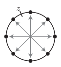
Figure 1. The antipodal pointed matched circle. The genus $2$ case is shown; the matching is indicated with gray arrows. See also [LOT08, Example 3.20].

We will prove two special cases of Conjecture 2:

Theorem 7.

Let $\mathcal{Z}$ be the antipodal pointed matched circle (Figure 1) for a surface of genus $k$. Then $\mathcal{A}(\mathcal{Z},-k+1)$ is $\pi$-formal.

Theorem 8.

Let $\mathcal{Z}$ be the antipodal pointed matched circle for a surface of genus $k\leq 2$. Then for any $i$, $\mathcal{A}(\mathcal{Z},i)$ is $\pi$-formal.

We start by proving Theorem 7, but first recall some facts about the algebra $\mathcal{A}=\mathcal{A}(\mathcal{Z},-k+1)$. The differential on $\mathcal{A}$ vanishes; and $\mathcal{A}$ has a simple description as a path algebra with relations:

$$\mathcal{A}=\Biggl{(}\lx@xy@svg{\hbox{\raise 0.0pt\hbox{\kern 6.16968pt\hbox{\ignorespaces\ignorespaces\ignorespaces\hbox{\vtop{\kern 0.0pt\offinterlineskip\halign{\entry@#!@&&\entry@@#!@\cr&&&\crcr}}}\ignorespaces{\hbox{\kern-6.16968pt\raise 0.0pt\hbox{\hbox{\kern 0.0pt\raise 0.0pt\hbox{\hbox{\kern 3.0pt\raise 0.0pt\hbox{$\textstyle{\iota_{1}\ignorespaces\ignorespaces\ignorespaces\ignorespaces\ignorespaces\ignorespaces\ignorespaces\ignorespaces\ignorespaces\ignorespaces}$}}}}}}}\ignorespaces\ignorespaces\ignorespaces\ignorespaces\ignorespaces{}{}{}{{}{}{}{}{}{}{}{}{}{}{}{}{}{}{}{}{}{}{}}{}\ignorespaces\hbox{\hbox{\kern 0.0pt\raise 0.0pt\hbox{{}{}{{}}{{}{}{}}{}}}}\ignorespaces{}\ignorespaces{}{}{}{{}{}}\ignorespaces\ignorespaces{\hbox{\kern 12.31963pt\raise 11.15138pt\hbox{{}\hbox{\kern 0.0pt\raise 0.0pt\hbox{\hbox{\kern 3.0pt\hbox{\hbox{\kern 0.0pt\raise-0.8625pt\hbox{$\scriptstyle{a_{1}}$}}}\kern 3.0pt}}}}}}\ignorespaces{}{}{}{{}{}{}{}{}{}{}{}{}{}{}{}{}{}{}{}{}{}}{\hbox{\kern 30.1734pt\raise 3.3813pt\hbox{\hbox{\kern 0.0pt\raise 0.0pt\hbox{\lx@xy@tip{1}\lx@xy@tip{-1}}}}}}\ignorespaces\hbox{\hbox{\kern 0.0pt\raise 0.0pt\hbox{{}{}{}{{}}{{}{}{}\lx@xy@spline@}{}}}}\ignorespaces{}\ignorespaces\hbox{\hbox{\kern 0.0pt\raise 0.0pt\hbox{{}{}{{}}{{}{}{}}{}}}}\ignorespaces{}\ignorespaces\ignorespaces\ignorespaces\ignorespaces\ignorespaces{}{}{}{{}{}{}{}{}{}{}{}{}{}{}{}{}{}{}{}{}{}{}}{}\ignorespaces\hbox{\hbox{\kern 0.0pt\raise 0.0pt\hbox{{}{}{{}}{{}{}{}}{}}}}\ignorespaces{}\ignorespaces{}{}{}{{}{}}\ignorespaces\ignorespaces{\hbox{\kern 12.6676pt\raise-12.07498pt\hbox{{}\hbox{\kern 0.0pt\raise 0.0pt\hbox{\hbox{\kern 3.0pt\hbox{\hbox{\kern 0.0pt\raise-1.78612pt\hbox{$\scriptstyle{b_{1}}$}}}\kern 3.0pt}}}}}}\ignorespaces{}{}{}{{}{}{}{}{}{}{}{}{}{}{}{}{}{}{}{}{}{}}{\hbox{\kern 30.1734pt\raise-3.3813pt\hbox{\hbox{\kern 0.0pt\raise 0.0pt\hbox{\lx@xy@tip{1}\lx@xy@tip{-1}}}}}}\ignorespaces\hbox{\hbox{\kern 0.0pt\raise 0.0pt\hbox{{}{}{}{{}}{{}{}{}\lx@xy@spline@}{}}}}\ignorespaces{}\ignorespaces\hbox{\hbox{\kern 0.0pt\raise 0.0pt\hbox{{}{}{{}}{{}{}{}}{}}}}\ignorespaces{}{\hbox{\kern 30.16968pt\raise 0.0pt\hbox{\hbox{\kern 0.0pt\raise 0.0pt\hbox{\hbox{\kern 3.0pt\raise 0.0pt\hbox{$\textstyle{\iota_{2}\ignorespaces\ignorespaces\ignorespaces\ignorespaces\ignorespaces\ignorespaces\ignorespaces\ignorespaces\ignorespaces\ignorespaces}$}}}}}}}\ignorespaces\ignorespaces\ignorespaces\ignorespaces\ignorespaces{}{}{}{{}{}{}{}{}{}{}{}{}{}{}{}{}{}{}}{}\ignorespaces\hbox{\hbox{\kern 0.0pt\raise 0.0pt\hbox{{}{}{{}}{{}{}{}}{}}}}\ignorespaces{}\ignorespaces{}{}{}{{}{}}\ignorespaces\ignorespaces{\hbox{\kern 48.94914pt\raise 11.15138pt\hbox{{}\hbox{\kern 0.0pt\raise 0.0pt\hbox{\hbox{\kern 3.0pt\hbox{\hbox{\kern 0.0pt\raise-0.8625pt\hbox{$\scriptstyle{a_{2}}$}}}\kern 3.0pt}}}}}}\ignorespaces{}{}{}{{}{}{}{}{}{}{}{}{}{}{}{}{}{}{}{}{}{}}{\hbox{\kern 66.5079pt\raise 3.58617pt\hbox{\hbox{\kern 0.0pt\raise 0.0pt\hbox{\lx@xy@tip{1}\lx@xy@tip{-1}}}}}}\ignorespaces\hbox{\hbox{\kern 0.0pt\raise 0.0pt\hbox{{}{}{}{{}}{{}{}{}\lx@xy@spline@}{}}}}\ignorespaces{}\ignorespaces\hbox{\hbox{\kern 0.0pt\raise 0.0pt\hbox{{}{}{{}}{{}{}{}}{}}}}\ignorespaces{}\ignorespaces\ignorespaces\ignorespaces\ignorespaces\ignorespaces{}{}{}{{}{}{}{}{}{}{}{}{}{}{}{}{}{}{}}{}\ignorespaces\hbox{\hbox{\kern 0.0pt\raise 0.0pt\hbox{{}{}{{}}{{}{}{}}{}}}}\ignorespaces{}\ignorespaces{}{}{}{{}{}}\ignorespaces\ignorespaces{\hbox{\kern 49.29712pt\raise-12.07498pt\hbox{{}\hbox{\kern 0.0pt\raise 0.0pt\hbox{\hbox{\kern 3.0pt\hbox{\hbox{\kern 0.0pt\raise-1.78612pt\hbox{$\scriptstyle{b_{2}}$}}}\kern 3.0pt}}}}}}\ignorespaces{}{}{}{{}{}{}{}{}{}{}{}{}{}{}{}{}{}{}{}{}{}}{\hbox{\kern 66.5079pt\raise-3.58617pt\hbox{\hbox{\kern 0.0pt\raise 0.0pt\hbox{\lx@xy@tip{1}\lx@xy@tip{-1}}}}}}\ignorespaces\hbox{\hbox{\kern 0.0pt\raise 0.0pt\hbox{{}{}{}{{}}{{}{}{}\lx@xy@spline@}{}}}}\ignorespaces{}\ignorespaces\hbox{\hbox{\kern 0.0pt\raise 0.0pt\hbox{{}{}{{}}{{}{}{}}{}}}}\ignorespaces{}{\hbox{\kern 66.50903pt\raise 0.0pt\hbox{\hbox{\kern 0.0pt\raise 0.0pt\hbox{\hbox{\kern 3.0pt\raise 0.0pt\hbox{$\textstyle{\cdots\ignorespaces\ignorespaces\ignorespaces\ignorespaces\ignorespaces\ignorespaces\ignorespaces\ignorespaces\ignorespaces\ignorespaces}$}}}}}}}\ignorespaces\ignorespaces\ignorespaces\ignorespaces\ignorespaces{}{}{}{{}{}{}{}{}{}{}{}{}{}{}{}{}{}{}{}{}{}{}}{}\ignorespaces\hbox{\hbox{\kern 0.0pt\raise 0.0pt\hbox{{}{}{{}}{{}{}{}}{}}}}\ignorespaces{}\ignorespaces{}{}{}{{}{}}\ignorespaces\ignorespaces{\hbox{\kern 83.87091pt\raise 11.20139pt\hbox{{}\hbox{\kern 0.0pt\raise 0.0pt\hbox{\hbox{\kern 3.0pt\hbox{\hbox{\kern 0.0pt\raise-0.8125pt\hbox{$\scriptstyle{a_{2k-1}}$}}}\kern 3.0pt}}}}}}\ignorespaces{}{}{}{{}{}{}{}{}{}{}{}{}{}{}{}{}{}{}{}{}{}{}{}}{\hbox{\kern 104.00992pt\raise 3.8481pt\hbox{\hbox{\kern 0.0pt\raise 0.0pt\hbox{\lx@xy@tip{1}\lx@xy@tip{-1}}}}}}\ignorespaces\hbox{\hbox{\kern 0.0pt\raise 0.0pt\hbox{{}{}{}{{}}{{}{}{}\lx@xy@spline@}{}}}}\ignorespaces{}\ignorespaces\hbox{\hbox{\kern 0.0pt\raise 0.0pt\hbox{{}{}{{}}{{}{}{}}{}}}}\ignorespaces{}\ignorespaces\ignorespaces\ignorespaces\ignorespaces\ignorespaces{}{}{}{{}{}{}{}{}{}{}{}{}{}{}{}{}{}{}{}{}{}{}}{}\ignorespaces\hbox{\hbox{\kern 0.0pt\raise 0.0pt\hbox{{}{}{{}}{{}{}{}}{}}}}\ignorespaces{}\ignorespaces{}{}{}{{}{}}\ignorespaces\ignorespaces{\hbox{\kern 84.21889pt\raise-12.12498pt\hbox{{}\hbox{\kern 0.0pt\raise 0.0pt\hbox{\hbox{\kern 3.0pt\hbox{\hbox{\kern 0.0pt\raise-1.73611pt\hbox{$\scriptstyle{b_{2k-1}}$}}}\kern 3.0pt}}}}}}\ignorespaces{}{}{}{{}{}{}{}{}{}{}{}{}{}{}{}{}{}{}{}{}{}{}{}}{\hbox{\kern 104.00992pt\raise-3.8481pt\hbox{\hbox{\kern 0.0pt\raise 0.0pt\hbox{\lx@xy@tip{1}\lx@xy@tip{-1}}}}}}\ignorespaces\hbox{\hbox{\kern 0.0pt\raise 0.0pt\hbox{{}{}{}{{}}{{}{}{}\lx@xy@spline@}{}}}}\ignorespaces{}\ignorespaces\hbox{\hbox{\kern 0.0pt\raise 0.0pt\hbox{{}{}{{}}{{}{}{}}{}}}}\ignorespaces{}{\hbox{\kern 104.00903pt\raise 0.0pt\hbox{\hbox{\kern 0.0pt\raise 0.0pt\hbox{\hbox{\kern 3.0pt\raise 0.0pt\hbox{$\textstyle{\iota_{2k}\ignorespaces\ignorespaces\ignorespaces\ignorespaces\ignorespaces}$}}}}}}}\ignorespaces\ignorespaces\ignorespaces\ignorespaces\ignorespaces{}{}{}{{}{}{}{}{}{}{}{}{}{}{}{}{}{}}{}\ignorespaces\hbox{\hbox{\kern 0.0pt\raise 0.0pt\hbox{{}{}{{}}{{}{}{}}{}}}}\ignorespaces{}\ignorespaces{}{}{}{{}{}}\ignorespaces\ignorespaces{\hbox{\kern 51.34764pt\raise-31.49306pt\hbox{{}\hbox{\kern 0.0pt\raise 0.0pt\hbox{\hbox{\kern 3.0pt\hbox{\hbox{\kern 0.0pt\raise-1.50694pt\hbox{$\scriptstyle{c}$}}}\kern 3.0pt}}}}}}\ignorespaces{}{}{}{{}{}{}{}{}{}{}{}{}{}{}{}{}{}{}{}{}{}{}{}{}{}}{\hbox{\kern 3.85965pt\raise-4.80276pt\hbox{\hbox{\kern 0.0pt\raise 0.0pt\hbox{\lx@xy@tip{1}\lx@xy@tip{-1}}}}}}\ignorespaces\hbox{\hbox{\kern 0.0pt\raise 0.0pt\hbox{{}{}{}{{}}{{}{}{}\lx@xy@spline@}{}}}}\ignorespaces{}\ignorespaces\hbox{\hbox{\kern 0.0pt\raise 0.0pt\hbox{{}{}{{}}{{}{}{}}{}}}}\ignorespaces{}\ignorespaces}}}}\ignorespaces\bigg{/}a_{i}b_{i+1}=b_{i}a_{i+1}=b_{2k-1}c=ca_{1}=0\Biggr{)}. \textstyle{\iota_{1}\ignorespaces\ignorespaces\ignorespaces\ignorespaces\ignorespaces\ignorespaces\ignorespaces\ignorespaces\ignorespaces\ignorespaces} \scriptstyle{a_{1}} \scriptstyle{b_{1}} \textstyle{\iota_{2}\ignorespaces\ignorespaces\ignorespaces\ignorespaces\ignorespaces\ignorespaces\ignorespaces\ignorespaces\ignorespaces\ignorespaces} \scriptstyle{a_{2}} \scriptstyle{b_{2}} \textstyle{\cdots\ignorespaces\ignorespaces\ignorespaces\ignorespaces\ignorespaces\ignorespaces\ignorespaces\ignorespaces\ignorespaces\ignorespaces} \scriptstyle{a_{2k-1}} \scriptstyle{b_{2k-1}} \textstyle{\iota_{2k}\ignorespaces\ignorespaces\ignorespaces\ignorespaces\ignorespaces} \scriptstyle{c} \textstyle{\iota_{1}\ignorespaces\ignorespaces\ignorespaces\ignorespaces\ignorespaces\ignorespaces\ignorespaces\ignorespaces\ignorespaces\ignorespaces} \scriptstyle{a_{1}} \scriptstyle{b_{1}} \textstyle{\iota_{2}\ignorespaces\ignorespaces\ignorespaces\ignorespaces\ignorespaces\ignorespaces\ignorespaces\ignorespaces\ignorespaces\ignorespaces} \scriptstyle{a_{2}} \scriptstyle{b_{2}} \textstyle{\cdots\ignorespaces\ignorespaces\ignorespaces\ignorespaces\ignorespaces\ignorespaces\ignorespaces\ignorespaces\ignorespaces\ignorespaces} \scriptstyle{a_{2k-1}} \scriptstyle{b_{2k-1}} \textstyle{\iota_{2k}\ignorespaces\ignorespaces\ignorespaces\ignorespaces\ignorespaces} \scriptstyle{c}$$

The algebra $\mathcal{A}$ is quadratic. Its quadratic dual is given by

$$\mathcal{B}=\Biggl{(}\lx@xy@svg{\hbox{\raise 0.0pt\hbox{\kern 6.16968pt\hbox{\ignorespaces\ignorespaces\ignorespaces\hbox{\vtop{\kern 0.0pt\offinterlineskip\halign{\entry@#!@&&\entry@@#!@\cr&&&\crcr}}}\ignorespaces{\hbox{\kern-6.16968pt\raise 0.0pt\hbox{\hbox{\kern 0.0pt\raise 0.0pt\hbox{\hbox{\kern 3.0pt\raise 0.0pt\hbox{$\textstyle{\iota_{1}\ignorespaces\ignorespaces\ignorespaces\ignorespaces\ignorespaces}$}}}}}}}\ignorespaces\ignorespaces\ignorespaces\ignorespaces\ignorespaces{}{}{}{{}{}{}{}{}{}{}{}{}{}{}{}{}{}{}}{}\ignorespaces\hbox{\hbox{\kern 0.0pt\raise 0.0pt\hbox{{}{}{{}}{{}{}{}}{}}}}\ignorespaces{}\ignorespaces{}{}{}{{}{}}\ignorespaces\ignorespaces{\hbox{\kern 50.79764pt\raise-41.0625pt\hbox{{}\hbox{\kern 0.0pt\raise 0.0pt\hbox{\hbox{\kern 3.0pt\hbox{\hbox{\kern 0.0pt\raise-2.0625pt\hbox{$\scriptstyle{c^{\prime}}$}}}\kern 3.0pt}}}}}}\ignorespaces{}{}{}{{}{}{}{}{}{}{}{}{}{}{}{}{}{}{}{}{}{}{}{}}{\hbox{\kern 107.74225pt\raise-4.94986pt\hbox{\hbox{\kern 0.0pt\raise 0.0pt\hbox{\lx@xy@tip{1}\lx@xy@tip{-1}}}}}}\ignorespaces\hbox{\hbox{\kern 0.0pt\raise 0.0pt\hbox{{}{}{}{{}}{{}{}{}\lx@xy@spline@}{}}}}\ignorespaces{}\ignorespaces\hbox{\hbox{\kern 0.0pt\raise 0.0pt\hbox{{}{}{{}}{{}{}{}}{}}}}\ignorespaces{}{\hbox{\kern 30.16968pt\raise 0.0pt\hbox{\hbox{\kern 0.0pt\raise 0.0pt\hbox{\hbox{\kern 3.0pt\raise 0.0pt\hbox{$\textstyle{\iota_{2}\ignorespaces\ignorespaces\ignorespaces\ignorespaces\ignorespaces\ignorespaces\ignorespaces\ignorespaces\ignorespaces\ignorespaces}$}}}}}}}\ignorespaces\ignorespaces\ignorespaces\ignorespaces\ignorespaces{}{}{}{{}{}{}{}{}{}{}{}{}{}{}{}{}{}{}{}{}{}{}}{}\ignorespaces\hbox{\hbox{\kern 0.0pt\raise 0.0pt\hbox{{}{}{{}}{{}{}{}}{}}}}\ignorespaces{}\ignorespaces{}{}{}{{}{}}\ignorespaces\ignorespaces{\hbox{\kern 12.76962pt\raise 11.70694pt\hbox{{}\hbox{\kern 0.0pt\raise 0.0pt\hbox{\hbox{\kern 3.0pt\hbox{\hbox{\kern 0.0pt\raise-1.41806pt\hbox{$\scriptstyle{a^{\prime}_{1}}$}}}\kern 3.0pt}}}}}}\ignorespaces{}{}{}{{}{}{}{}{}{}{}{}{}{}{}{}{}{}{}{}{}{}}{\hbox{\kern 6.16605pt\raise 3.3813pt\hbox{\hbox{\kern 0.0pt\raise 0.0pt\hbox{\lx@xy@tip{1}\lx@xy@tip{-1}}}}}}\ignorespaces\hbox{\hbox{\kern 0.0pt\raise 0.0pt\hbox{{}{}{}{{}}{{}{}{}\lx@xy@spline@}{}}}}\ignorespaces{}\ignorespaces\hbox{\hbox{\kern 0.0pt\raise 0.0pt\hbox{{}{}{{}}{{}{}{}}{}}}}\ignorespaces{}\ignorespaces\ignorespaces\ignorespaces\ignorespaces\ignorespaces{}{}{}{{}{}{}{}{}{}{}{}{}{}{}{}{}{}{}{}{}{}{}}{}\ignorespaces\hbox{\hbox{\kern 0.0pt\raise 0.0pt\hbox{{}{}{{}}{{}{}{}}{}}}}\ignorespaces{}\ignorespaces{}{}{}{{}{}}\ignorespaces\ignorespaces{\hbox{\kern 13.1176pt\raise-12.63054pt\hbox{{}\hbox{\kern 0.0pt\raise 0.0pt\hbox{\hbox{\kern 3.0pt\hbox{\hbox{\kern 0.0pt\raise-2.34167pt\hbox{$\scriptstyle{b^{\prime}_{1}}$}}}\kern 3.0pt}}}}}}\ignorespaces{}{}{}{{}{}{}{}{}{}{}{}{}{}{}{}{}{}{}{}{}{}}{\hbox{\kern 6.16605pt\raise-3.3813pt\hbox{\hbox{\kern 0.0pt\raise 0.0pt\hbox{\lx@xy@tip{1}\lx@xy@tip{-1}}}}}}\ignorespaces\hbox{\hbox{\kern 0.0pt\raise 0.0pt\hbox{{}{}{}{{}}{{}{}{}\lx@xy@spline@}{}}}}\ignorespaces{}\ignorespaces\hbox{\hbox{\kern 0.0pt\raise 0.0pt\hbox{{}{}{{}}{{}{}{}}{}}}}\ignorespaces{}{\hbox{\kern 66.50903pt\raise 0.0pt\hbox{\hbox{\kern 0.0pt\raise 0.0pt\hbox{\hbox{\kern 3.0pt\raise 0.0pt\hbox{$\textstyle{\cdots\ignorespaces\ignorespaces\ignorespaces\ignorespaces\ignorespaces\ignorespaces\ignorespaces\ignorespaces\ignorespaces\ignorespaces}$}}}}}}}\ignorespaces\ignorespaces\ignorespaces\ignorespaces\ignorespaces{}{}{}{{}{}{}{}{}{}{}{}{}{}{}{}{}{}{}{}{}{}{}}{}\ignorespaces\hbox{\hbox{\kern 0.0pt\raise 0.0pt\hbox{{}{}{{}}{{}{}{}}{}}}}\ignorespaces{}\ignorespaces{}{}{}{{}{}}\ignorespaces\ignorespaces{\hbox{\kern 49.39914pt\raise 11.70694pt\hbox{{}\hbox{\kern 0.0pt\raise 0.0pt\hbox{\hbox{\kern 3.0pt\hbox{\hbox{\kern 0.0pt\raise-1.41806pt\hbox{$\scriptstyle{a^{\prime}_{2}}$}}}\kern 3.0pt}}}}}}\ignorespaces{}{}{}{{}{}{}{}{}{}{}{}{}{}{}{}{}{}{}{}}{\hbox{\kern 42.5047pt\raise 3.33855pt\hbox{\hbox{\kern 0.0pt\raise 0.0pt\hbox{\lx@xy@tip{1}\lx@xy@tip{-1}}}}}}\ignorespaces\hbox{\hbox{\kern 0.0pt\raise 0.0pt\hbox{{}{}{}{{}}{{}{}{}\lx@xy@spline@}{}}}}\ignorespaces{}\ignorespaces\hbox{\hbox{\kern 0.0pt\raise 0.0pt\hbox{{}{}{{}}{{}{}{}}{}}}}\ignorespaces{}\ignorespaces\ignorespaces\ignorespaces\ignorespaces\ignorespaces{}{}{}{{}{}{}{}{}{}{}{}{}{}{}{}{}{}{}{}{}{}{}}{}\ignorespaces\hbox{\hbox{\kern 0.0pt\raise 0.0pt\hbox{{}{}{{}}{{}{}{}}{}}}}\ignorespaces{}\ignorespaces{}{}{}{{}{}}\ignorespaces\ignorespaces{\hbox{\kern 49.74712pt\raise-12.63054pt\hbox{{}\hbox{\kern 0.0pt\raise 0.0pt\hbox{\hbox{\kern 3.0pt\hbox{\hbox{\kern 0.0pt\raise-2.34167pt\hbox{$\scriptstyle{b^{\prime}_{2}}$}}}\kern 3.0pt}}}}}}\ignorespaces{}{}{}{{}{}{}{}{}{}{}{}{}{}{}{}{}{}{}{}}{\hbox{\kern 42.5047pt\raise-3.33855pt\hbox{\hbox{\kern 0.0pt\raise 0.0pt\hbox{\lx@xy@tip{1}\lx@xy@tip{-1}}}}}}\ignorespaces\hbox{\hbox{\kern 0.0pt\raise 0.0pt\hbox{{}{}{}{{}}{{}{}{}\lx@xy@spline@}{}}}}\ignorespaces{}\ignorespaces\hbox{\hbox{\kern 0.0pt\raise 0.0pt\hbox{{}{}{{}}{{}{}{}}{}}}}\ignorespaces{}{\hbox{\kern 104.00903pt\raise 0.0pt\hbox{\hbox{\kern 0.0pt\raise 0.0pt\hbox{\hbox{\kern 3.0pt\raise 0.0pt\hbox{$\textstyle{\iota_{2k}\ignorespaces\ignorespaces\ignorespaces\ignorespaces\ignorespaces\ignorespaces\ignorespaces\ignorespaces\ignorespaces\ignorespaces}$}}}}}}}\ignorespaces\ignorespaces\ignorespaces\ignorespaces\ignorespaces{}{}{}{{}{}{}{}{}{}{}{}{}{}{}{}{}{}{}{}{}}{}\ignorespaces\hbox{\hbox{\kern 0.0pt\raise 0.0pt\hbox{{}{}{{}}{{}{}{}}{}}}}\ignorespaces{}\ignorespaces{}{}{}{{}{}}\ignorespaces\ignorespaces{\hbox{\kern 87.09174pt\raise 11.75694pt\hbox{{}\hbox{\kern 0.0pt\raise 0.0pt\hbox{\hbox{\kern 3.0pt\hbox{\hbox{\kern 0.0pt\raise-1.36806pt\hbox{$\scriptstyle{a^{\prime}_{2k-1}}$}}}\kern 3.0pt}}}}}}\ignorespaces{}{}{}{{}{}{}{}{}{}{}{}{}{}{}{}{}{}{}{}{}{}}{\hbox{\kern 80.01123pt\raise 3.47339pt\hbox{\hbox{\kern 0.0pt\raise 0.0pt\hbox{\lx@xy@tip{1}\lx@xy@tip{-1}}}}}}\ignorespaces\hbox{\hbox{\kern 0.0pt\raise 0.0pt\hbox{{}{}{}{{}}{{}{}{}\lx@xy@spline@}{}}}}\ignorespaces{}\ignorespaces\hbox{\hbox{\kern 0.0pt\raise 0.0pt\hbox{{}{}{{}}{{}{}{}}{}}}}\ignorespaces{}\ignorespaces\ignorespaces\ignorespaces\ignorespaces\ignorespaces{}{}{}{{}{}{}{}{}{}{}{}{}{}{}{}{}{}{}{}{}}{}\ignorespaces\hbox{\hbox{\kern 0.0pt\raise 0.0pt\hbox{{}{}{{}}{{}{}{}}{}}}}\ignorespaces{}\ignorespaces{}{}{}{{}{}}\ignorespaces\ignorespaces{\hbox{\kern 87.43971pt\raise-12.68054pt\hbox{{}\hbox{\kern 0.0pt\raise 0.0pt\hbox{\hbox{\kern 3.0pt\hbox{\hbox{\kern 0.0pt\raise-2.29167pt\hbox{$\scriptstyle{b^{\prime}_{2k-1}}$}}}\kern 3.0pt}}}}}}\ignorespaces{}{}{}{{}{}{}{}{}{}{}{}{}{}{}{}{}{}{}{}{}{}}{\hbox{\kern 80.01123pt\raise-3.47339pt\hbox{\hbox{\kern 0.0pt\raise 0.0pt\hbox{\lx@xy@tip{1}\lx@xy@tip{-1}}}}}}\ignorespaces\hbox{\hbox{\kern 0.0pt\raise 0.0pt\hbox{{}{}{}{{}}{{}{}{}\lx@xy@spline@}{}}}}\ignorespaces{}\ignorespaces\hbox{\hbox{\kern 0.0pt\raise 0.0pt\hbox{{}{}{{}}{{}{}{}}{}}}}\ignorespaces{}\ignorespaces}}}}\ignorespaces\bigg{/}a^{\prime}_{i}a^{\prime}_{i+1}=b^{\prime}_{i}b^{\prime}_{i+1}=c^{\prime}a^{\prime}_{2k-1}=b^{\prime}_{1}c^{\prime}=0\Biggr{)}. \textstyle{\iota_{1}\ignorespaces\ignorespaces\ignorespaces\ignorespaces\ignorespaces} \scriptstyle{c^{\prime}} \textstyle{\iota_{2}\ignorespaces\ignorespaces\ignorespaces\ignorespaces\ignorespaces\ignorespaces\ignorespaces\ignorespaces\ignorespaces\ignorespaces} \scriptstyle{a^{\prime}_{1}} \scriptstyle{b^{\prime}_{1}} \textstyle{\cdots\ignorespaces\ignorespaces\ignorespaces\ignorespaces\ignorespaces\ignorespaces\ignorespaces\ignorespaces\ignorespaces\ignorespaces} \scriptstyle{a^{\prime}_{2}} \scriptstyle{b^{\prime}_{2}} \textstyle{\iota_{2k}\ignorespaces\ignorespaces\ignorespaces\ignorespaces\ignorespaces\ignorespaces\ignorespaces\ignorespaces\ignorespaces\ignorespaces} \scriptstyle{a^{\prime}_{2k-1}} \scriptstyle{b^{\prime}_{2k-1}} \textstyle{\iota_{1}\ignorespaces\ignorespaces\ignorespaces\ignorespaces\ignorespaces} \scriptstyle{c^{\prime}} \textstyle{\iota_{2}\ignorespaces\ignorespaces\ignorespaces\ignorespaces\ignorespaces\ignorespaces\ignorespaces\ignorespaces\ignorespaces\ignorespaces} \scriptstyle{a^{\prime}_{1}} \scriptstyle{b^{\prime}_{1}} \textstyle{\cdots\ignorespaces\ignorespaces\ignorespaces\ignorespaces\ignorespaces\ignorespaces\ignorespaces\ignorespaces\ignorespaces\ignorespaces} \scriptstyle{a^{\prime}_{2}} \scriptstyle{b^{\prime}_{2}} \textstyle{\iota_{2k}\ignorespaces\ignorespaces\ignorespaces\ignorespaces\ignorespaces\ignorespaces\ignorespaces\ignorespaces\ignorespaces\ignorespaces} \scriptstyle{a^{\prime}_{2k-1}} \scriptstyle{b^{\prime}_{2k-1}}$$

(In fact, $\mathcal{A}$ and $\mathcal{B}$ are isomorphic, but it will be clearer to view them as distinct.)

The following is essentially a special case of results from [LOT11]:

Proposition 4.15.

The algebra $\mathcal{A}$ is Koszul (over its subalgebra $\mathbf{k}$ of idempotents).

Proof.

Given a pointed matched circle $\mathcal{Z}$, we can form $-\mathcal{Z}$, the orientation-reverse of $\mathcal{Z}$. We can also form the dual pointed matched circle $\mathcal{Z}_{*}$: if we think of $\mathcal{Z}$ as a handle decomposition coming from a Morse function $f\nobreak\mskip 2.0mu\mathpunct{}\nonscript\mkern-3.0mu{:}\penalty 300\mskip 6.0mu plus 1.0muF(\mathcal{Z})\to\mathbb{R}$ then $\mathcal{Z}_{*}$ corresponds to $-f$. The algebra $\mathcal{B}$ is simply $\mathcal{A}(\mathcal{Z}_{*},-k+1)$. It is explained in [LOT11, Section 8.2] that $\mathcal{A}(\mathcal{Z},i)$ is Koszul dual (in a particular sense) to both $\mathcal{A}(-\mathcal{Z},-i)$ and $\mathcal{A}(\mathcal{Z}_{*},i)$. So, the work in proving the present proposition is simply translating that result into the language of this paper.

As in the proof of [LOT11, Theorem 13], consider the type DD bimodule ${}^{\mathcal{A}}\mskip-1.80002mu\textit{DD}(\frac{\mathbb{I}}{2})^{\mathcal{B}}$ associated to the diagram $\mathcal{G}(\mathcal{Z})$ of [LOT11, Construction 8.18]. By [LOT11, Proposition 8.13] and the proof of [LOT11, Theorem 13], ${}_{\mathcal{A}}\mathcal{A}_{\mathcal{A}}\boxtimes{}^{\mathcal{A}}\mskip-1.80002mu\textit{DD}(\frac{\mathbb{I}}{2})^{\mathcal{B}}\boxtimes{}_{\mathcal{B}}\mathcal{B}$ is a resolution of $\mathbf{k}$. But the bimodule ${}^{\mathcal{A}}\mskip-1.80002mu\textit{DD}(\frac{\mathbb{I}}{2})^{\mathcal{B}}$ is computed explicitly in [LOT13, Proposition 3.22]; in particular, it follows from that description that ${}_{\mathcal{A}}\mathcal{A}_{\mathcal{A}}\boxtimes{}^{\mathcal{A}}\mskip-1.80002mu\textit{DD}(\frac{\mathbb{I}}{2})^{\mathcal{B}}\boxtimes\mathcal{B}$ is the Koszul complex. ∎

In particular, the Koszul resolution of $\mathcal{A}$ is given by $\mathcal{A}\otimes\mathcal{B}^{*}\otimes\mathcal{A}$, with differential

$$\partial(x\otimes f\otimes z) =\sum_{i=1}^{2k-1}(xa_{i}\otimes a^{\prime}_{i}f\otimes z+xb_{i}\otimes b^{\prime}_{i}f\otimes z+x\otimes fa^{\prime}_{i}\otimes a_{i}z+x\otimes fb^{\prime}_{i}\otimes b_{i}z)$$

$$\qquad\qquad+xc\otimes c^{\prime}f\otimes z+x\otimes fc^{\prime}\otimes cz.$$

(Here, in Corollary 4.16, and in the proof of Theorem 7, $\otimes$ means the tensor product over $\mathbf{k}$, the subalgebra of idempotents. In particular, we are using the identification between the idempotents of $\mathcal{A}$ and $\mathcal{B}$ given by the labeling of vertices in the path algebra description above.)

Using this Koszul resolution, we get a model for $A^{!}$:

$$A^{!}=\operatorname{Hom}_{{}_{A}\mathsf{Mod}_{A}}((\mathcal{A}\otimes\mathcal{B}^{*}\otimes\mathcal{A},\partial),\mathcal{A}^{e})=(\mathcal{A}\otimes\mathcal{B}\otimes\mathcal{A},\partial^{T})$$

(see Section 3.1.3), where $\partial^{T}$ denotes map induced by $\partial$. Using this model, we have:

Corollary 4.16.

The Hochschild homology of $\mathcal{A}^{!}$ is the homology of the chain complex $\mathcal{A}\otimes\mathcal{B}/\sim$, where $x\otimes y\iota\sim\iota x\otimes y$ for each idempotent $\iota$, with differential

(4.17) $$\partial(x\otimes y)=\sum_{i=1}^{2k-1}(xa_{i}\otimes a^{\prime}_{i}y+a_{i}x\otimes ya^{\prime}_{i}+xb_{i}\otimes b^{\prime}_{i}y+b_{i}x\otimes yb^{\prime}_{i})+xc\otimes c^{\prime}y+cx\otimes yc^{\prime}.$$

Similarly, $\mathit{HH}_{*}(\mathcal{A}^{!}\otimes^{L}_{\mathcal{A}}\mathcal{A}^{!})$ is given by $\mathcal{A}\otimes\mathcal{B}\otimes\mathcal{A}\otimes\mathcal{B}/\sim$, where $x_{1}\otimes y_{1}\otimes x_{2}\otimes y_{2}\iota\sim\iota x_{1}\otimes y_{1}\otimes x_{2}\otimes y_{2}$ for each idempotent $\iota$, with differential

(4.18) $$\begin{split}\partial(x_{1}\otimes y_{1}\otimes x_{2}\otimes y_{2})&=\sum_{(\xi,\xi^{\prime})\in\{(a_{i},a^{\prime}_{i}),(b_{i},b^{\prime}_{i}),(c,c^{\prime})\}}(x_{1}\xi\otimes\xi^{\prime}y_{1}\otimes x_{2}\otimes y_{2}+x_{1}\otimes y_{1}\xi^{\prime}\otimes\xi x_{2}\otimes y_{2}\\ &\qquad\qquad\qquad+x_{1}\otimes y_{1}\otimes x_{2}\xi\otimes\xi^{\prime}y_{2}+\xi x_{1}\otimes y_{1}\otimes x_{2}\otimes y_{2}\xi^{\prime}).\end{split}$$

Proof of Theorem 7.

This is a somewhat long, concrete computation. To keep notation shorter, we will replace the symbol $\otimes$ with a vertical bar $|$. Similarly, let $\ell=2k-1$.

In the computation, we will frequently use the following phenomenon:

Vanishing phenomenon. If $\xi,\eta\in\{a_{i},b_{i},c\}$ then $\xi\eta\neq 0$ implies that $\eta^{\prime}\xi^{\prime}=0$. So, $\xi\eta|\eta^{\prime}\xi^{\prime}$ always vanishes, as does $\eta^{\prime}\xi^{\prime}|\xi\eta$.

The element $(1|1)$ in the model for $\mathit{HC}_{*}(\mathcal{A}^{!})$ given in Formula (4.17) corresponds to the element $1\in\operatorname{Hom}(A^{!},A^{!})$, and so we want to show that the elements $d^{2i}(1|1)$ vanish for all $i\geq 2$. To this end, consider the element $(1|1|1|1)$ in the model for $\mathit{HC}_{*}(\mathcal{A}^{!}\otimes^{L}\mathcal{A}^{!})$ given in Formula (4.18); note that $(1|1|1|1)$ corresponds to $(1|1)$ under the isomorphism of Proposition 3.10. We will compute the differentials in the spectral sequence as in Remark 3.4.

We have

(4.19) $$\partial(1|1|1|1) =\sum_{\xi\in\{a_{i},b_{i},c\}}(\xi|\xi^{\prime}|1|1)+(1|\xi^{\prime}|\xi|1)+(1|1|\xi|\xi^{\prime})+(\xi|1|1|\xi^{\prime})$$

(4.20) $$=(1+\tau)\bigl{(}\sum_{\xi\in\{a_{i},b_{i},c\}}(\xi|\xi^{\prime}|1|1)+(1|\xi^{\prime}|\xi|1)\bigr{)}.$$

Let $(1+\tau)^{-1}\eqref{eq:d1}$ denote the result of dropping the $(1+\tau)$ from Formula (4.20). Then

$$\partial\circ(1+\tau)^{-1}\eqref{eq:d1} =\sum_{\xi,\eta\in\{a_{i},b_{i},c\}}(\xi\eta|\eta^{\prime}\xi^{\prime}|1|1)+(\xi|\xi^{\prime}\eta^{\prime}|\eta|1)+(\xi|\xi^{\prime}|\eta|\eta^{\prime})+(\eta\xi|\xi^{\prime}|1|\eta^{\prime})$$

(4.21) $$\qquad\qquad\qquad\qquad+(\eta|\xi^{\prime}|\xi|\eta^{\prime})+(\eta|\eta^{\prime}\xi^{\prime}|\xi|1)+(1|\xi^{\prime}\eta^{\prime}|\eta\xi|1)+(1|\xi^{\prime}|\xi\eta|\eta^{\prime}).$$

In Expression (4.21), the first and seventh terms are identically zero, by the vanishing phenomenon above. When summing over $\xi$ and $\eta$, the second and sixth cancel. The sum over $\xi$ and $\eta$ of the eighth term is equal to tau applied to the sum over $\xi$ and $\eta$ of the fourth term. Further:

$$\sum_{\xi,\eta}(\xi|\xi^{\prime}|\eta|\eta^{\prime}) =\sum_{i=1}^{\ell}(a_{i}|a^{\prime}_{i}|a_{i}|a^{\prime}_{i})+(a_{i}|a^{\prime}_{i}|b_{i}|b^{\prime}_{i})+(b_{i}|b^{\prime}_{i}|a_{i}|a^{\prime}_{i})+(b_{i}|b^{\prime}_{i}|b_{i}|b^{\prime}_{i})$$

$$\sum_{\xi,\eta}(\eta|\xi^{\prime}|\xi|\eta^{\prime}) =\sum_{i=1}^{\ell}(a_{i}|a^{\prime}_{i}|a_{i}|a^{\prime}_{i})+(a_{i}|b^{\prime}_{i}|b_{i}|a^{\prime}_{i})+(b_{i}|a^{\prime}_{i}|a_{i}|b^{\prime}_{i})+(b_{i}|b^{\prime}_{i}|b_{i}|b^{\prime}_{i})$$

$$\sum_{\xi,\eta}(\xi|\xi^{\prime}|\eta|\eta^{\prime})+(\eta|\xi^{\prime}|\xi|\eta^{\prime}) =\sum_{i=1}^{\ell}(a_{i}|a^{\prime}_{i}|b_{i}|b^{\prime}_{i})+(b_{i}|b^{\prime}_{i}|a_{i}|a^{\prime}_{i})+(a_{i}|b^{\prime}_{i}|b_{i}|a^{\prime}_{i})+(b_{i}|a^{\prime}_{i}|a_{i}|b^{\prime}_{i}).$$

(In verifying these equations, keep in mind that we are tensoring over the idempotents.) Substituting in, we have:

(4.22) $$\eqref{eq:d1bdy}=(1+\tau)\bigl{(}\sum_{\xi,\eta}(\eta\xi|\xi^{\prime}|1|\eta^{\prime})+\sum_{i=1}^{\ell}(a_{i}|a^{\prime}_{i}|b_{i}|b^{\prime}_{i})+(b_{i}|a^{\prime}_{i}|a_{i}|b^{\prime}_{i})\bigr{)}.$$

Differentiating again,

(4.23) $$\begin{split}\partial\circ(&1+\tau)^{-1}\eqref{eq:d2}\\ &=\sum_{\eta,\xi,\nu\in\{a_{i},b_{i},c\}}(\eta\xi\nu|\nu^{\prime}\xi^{\prime}|1|\eta^{\prime})+(\eta\xi|\xi^{\prime}\nu^{\prime}|\nu|\eta^{\prime})+(\eta\xi|\xi^{\prime}|\nu|\nu^{\prime}\eta^{\prime})+(\nu\eta\xi|\xi^{\prime}|1|\eta^{\prime}\nu^{\prime})\\ &+\sum_{\nu\in\{a_{i},b_{i},c\}}\sum_{i=1}^{\ell}(a_{i}|a^{\prime}_{i}\nu|\nu b_{i}|b^{\prime}_{i})+(\nu a_{i}|a^{\prime}_{i}|b_{i}|b^{\prime}_{i}\nu)+(a_{i}\nu|\nu b^{\prime}_{i}|b_{i}|a^{\prime}_{i})+(a^{\prime}_{i}|b^{\prime}_{i}|b_{i}\nu|\nu a^{\prime}_{i}).\end{split}$$

Here, we have omitted some terms from the second sum which are zero according to the vanishing principle above (e.g., $(a_{i}\nu|\nu a^{\prime}_{i}|b_{i}|b^{\prime}_{i})$). In Formula (4.23), the first and fourth terms vanish identically, by the vanishing principle. Next:

$$\sum_{\eta,\xi,\nu}(\eta\xi|\xi^{\prime}\nu^{\prime}|\nu|\eta^{\prime}) =(a_{\ell}c|c^{\prime}b^{\prime}_{\ell}|b_{\ell}|a^{\prime}_{\ell})+\sum_{i=1}^{\ell-1}(a_{i}a_{i+1}|a^{\prime}_{i+1}b^{\prime}_{i}|b_{i}|a^{\prime}_{i})+(b_{i}b_{i+1}|b^{\prime}_{i+1}a^{\prime}_{i}|a_{i}|b^{\prime}_{i})$$

$$\sum_{\eta,\xi,\nu}(\eta\xi|\xi^{\prime}|\nu|\nu^{\prime}\eta^{\prime}) =(cb_{1}|b^{\prime}_{1}|a_{1}|a^{\prime}_{1}c^{\prime})+\sum_{i=1}^{\ell-1}(a_{i}a_{i+1}|a^{\prime}_{i+1}|b_{i+1}|b^{\prime}_{i+1}a^{\prime}_{i})+(b_{i}b_{i+1}|b^{\prime}_{i+1}|a_{i+1}|a^{\prime}_{i+1}b^{\prime}_{i})$$

and

$$\sum_{\nu}\sum_{i=1}^{\ell}(a_{i}|a^{\prime}_{i}\nu|\nu b_{i}|b^{\prime}_{i}) +(\nu a_{i}|a^{\prime}_{i}|b_{i}|b^{\prime}_{i}\nu)$$

$$\quad=(a_{1}|a^{\prime}_{1}c^{\prime}|cb_{1}|b^{\prime}_{1})+\sum_{i=1}^{\ell-1}(a_{i+1}|a^{\prime}_{i+1}b^{\prime}_{i}|b_{i}b_{i+1}|b^{\prime}_{i+1})+(a_{i}a_{i+1}|a^{\prime}_{i+1}|b_{i+1}|b^{\prime}_{i+1}a^{\prime}_{i})$$

$$\sum_{\nu}\sum_{i=1}^{\ell}(a_{i}\nu|\nu b^{\prime}_{i}|b_{i}|a^{\prime}_{i}) +(a^{\prime}_{i}|b^{\prime}_{i}|b_{i}\nu|\nu a^{\prime}_{i})$$

$$\quad=(a_{\ell}c|c^{\prime}b^{\prime}_{\ell}|b_{\ell}|a^{\prime}_{\ell})+\sum_{i=1}^{\ell-1}(a_{i}a_{i+1}|a^{\prime}_{i+1}b^{\prime}_{i}|b_{i}|a^{\prime}_{i})+(a_{i}|b^{\prime}_{i}|b_{i}b_{i+1}|b^{\prime}_{i+1}a^{\prime}_{i}).$$

So,

(4.24) $$\eqref{eq:d2bdy}=(1+\tau)\bigl{(}(a_{1}|a^{\prime}_{1}c^{\prime}|cb_{1}|b^{\prime}_{1})+\sum_{i=1}^{\ell-1}(a_{i+1}|a^{\prime}_{i+1}b^{\prime}_{i}|b_{i}b_{i+1}|b^{\prime}_{i+1})+(a_{i}|b^{\prime}_{i}|b_{i}b_{i+1}|b^{\prime}_{i+1}a^{\prime}_{i})\bigr{)}.$$

Finally,

$$\partial\circ(1+\tau)^{-1}\eqref{eq:d2bdy-v2} =\sum_{i=1}^{\ell-1}(a_{i}a_{i+1}|a^{\prime}_{i+1}b^{\prime}_{i}|b_{i}b_{i+1}|b^{\prime}_{i+1}a^{\prime}_{i})+(a_{i}a_{i+1}|a^{\prime}_{i+1}b^{\prime}_{i}|b_{i}b_{i+1}|b^{\prime}_{i+1}a^{\prime}_{i})$$

$$=0.\qed$$

Proof of Theorem 8.

The cases $k=0$, $k=1,i\neq 0$, and $k=1,i\not\in\{-1,0,1\}$ are trivial (the algebras are either $0$ or ${\mathbb{F}_{2}}$). The cases $(k,i)=(1,0)$ and $(2,-1)$ follow from Theorem 8. The case $(k,i)=(2,1)$ follows from Theorem 8 and the fact that $\mathcal{A}(\mathcal{Z},i)$ is quasi-isomorphic to $\mathcal{A}(\mathcal{Z}_{*},-i)$, which in turn is a special case of [LOT11, Theorem 13] and the fact that for the antipodal pointed matched circle $\mathcal{Z}$, $\mathcal{Z}=\mathcal{Z}_{*}$. So, only the case $k=2$, $i=0$ remains. This can be checked by computer, as follows. The proof of Proposition 4.1 gives a small model for the bar complex (first appearing in [LOT11, Section 5.4]), which in turn gives a model for the Hochschild cochain complex of $\mathcal{A}(\mathcal{Z},0)$. Explicitly, this cochain complex is $\mathcal{A}(\mathcal{Z},0)\otimes\mathcal{A}(-\mathcal{Z},0)$, with differential given by

$$\partial(x\otimes y)=\sum_{\text{chords }\xi}xa(\xi)\otimes a(\xi)y+a(\xi)x\otimes ya(\xi).$$

There is an analogous model for $\mathit{HC}_{*}(\mathcal{A}(\mathcal{Z},0)^{!}\otimes^{L}\mathcal{A}(\mathcal{Z},0)^{!})$. We are then interested in repeatedly applying $\partial$ and $(1+\tau)^{-1}$ to the element $e_{0}:=(1|1|1|1)$, as in the proof of Theorem 7. A computer calculation then gives the following:

• $\partial e_{0}\in\mathit{HC}_{-1}(\mathcal{A}(\mathcal{Z},0)^{!}\otimes^{L}\mathcal{A}(\mathcal{Z},0)^{!})$ is supported on 192 basis elements, and $\partial e_{0}=(1+\tau)(e_{1})$ for an element $e_{1}\in\mathit{HC}_{-1}$ supported on 96 basis elements.

• $\partial(e_{1})\in\mathit{HC}_{-2}$ is supported on $1176$ basis elements, and $\partial(e_{1})=(1+\tau)(e_{2}^{\prime})$ for an element $e_{2}^{\prime}\in\mathit{HC}_{-2}$ supported on 588 basis elements. (We eventually have to modify this lift of $\partial(e_{1})$, which is why we call it $e_{2}^{\prime}$.)

• $\partial(e_{2}^{\prime})\in\mathit{HC}_{-3}$ is supported on $2106$ elements, and $\partial(e_{2}^{\prime})=(1+\tau)(e_{3}^{\prime})$ for an element $e_{3}^{\prime}\in\mathit{HC}_{-3}$ supported on $1053$ basis elements. However $\partial(e_{3}^{\prime})$ is not in the image of $(1+\tau)$.

• There is an element $x\in\mathit{HC}_{-2}$ which is supported on 16 “square” basis elements (elements of the form $(a|b|a|b)$), and $e_{2}:=e_{2}^{\prime}+x$ has $(1+\tau)(e_{2})=\partial(e_{1})$ and $\partial(e_{2})\in\mathit{HC}_{-3}$ is supported on 2250 elements. Moreover $\partial(e_{2})=(1+\tau)(e_{3})$ for an element $e_{3}$ supported on $1125$ basis elements.

• $\partial e_{3}\in\mathit{HC}_{-4}$ is supported on $3092$ basis elements. Moreover $\partial e_{3}=(1+\tau)(e_{4}^{\prime})$ for an element $e_{4}^{\prime}\in\mathit{HC}_{-4}$ supported on $1546$ basis elements. This shows that the differential $d^{4}$ vanishes on $(1|1|1|1)$.

• $\partial e_{4}^{\prime}\in\mathit{HC}_{-5}$ is supported on $1944$ basis elements, and $\partial e_{4}^{\prime}=(1+\tau)(e_{5}^{\prime})$ for $e_{5}^{\prime}\in\mathit{HC}_{-5}$ supported on $972$ basis elements. However, $\partial e_{5}^{\prime}$ is not in the image of $(1+\tau)$.

• There is an element $y\in\mathit{HC}_{-4}$ supported on $24$ square basis elements, and $e_{4}=e_{4}^{\prime}+y$ has $(1+\tau)(e_{4})=\partial(e_{3})$ and $\partial(e_{4})\in\mathit{HC}_{-5}$ is supported on $2048$ basis elements. Moreover $\partial(e_{4})=(1+\tau)(e_{5})$ for an element $e_{5}$ supported on $1024$ basis elements.

• $\partial e_{5}$ is supported on $788$ basis elements, and $\partial e_{5}=(1+\tau)(e_{6})$ for an element $e_{6}$ supported on $394$ basis elements. This shows that $d^{6}$ vanishes on $(1|1|1|1)$.

The same computer code can be used to find $\mathit{HH}_{j}(\mathcal{A}(\mathcal{Z},0)^{!})$, in fact

$$\mathit{HH}_{0}={\mathbb{F}_{2}}\quad\mathit{HH}_{-1}=\mathbb{F}_{2}^{4}\quad\mathit{HH}_{-2}=\mathbb{F}_{2}^{10}\quad\mathit{HH}_{-3}={\mathbb{F}_{2}}$$

and all other groups vanish. By Proposition 3.12, it follows that $d^{2i}$ vanishes for $i>3$ and the Theorem is proved. Computer code is available from

http://math.columbia.edu/~lipshitz/BordHochLoc.tar. ∎

We conclude this section by observing that to obtain localization results, it suffices to show that the relevant bimodules are neutral (Definition 3.17):

Proposition 4.25.

For any pointed matched circle $\mathcal{Z}$ and any integer $i$, the Hochschild homology $\mathit{HH}_{*}(\mathcal{A}(\mathcal{Z},i))$ is supported in a single grading.

Proof.

Suppose that $\mathcal{Z}$ represents a surface of genus $k$. By Theorem 4.4, $\mathit{HH}_{*}(\mathcal{A}(\mathcal{Z},i))$ is the knot Floer homology of the $k^{\text{th}}$ Borromean knot (in $\#^{2k}(S^{2}\times S^{1})$) in the $i^{\text{th}}$ Alexander grading. So, the result follows from the computation of $\widehat{\mathit{HFK}}(B_{k})$ [OSz04, Section 9]. ∎

Corollary 4.26.

Every neutral $(\mathcal{A}(\mathcal{Z}),\mathcal{A}(\mathcal{Z}))$-bimodule is $\pi$-formal.

Proof.

This is immediate from Proposition 4.25 and Corollary 3.20. ∎

4.3. Branched double covers of links

As an expository point, we explain how Conjecture 2 implies [Hen12, Theorem 1.1]:

Theorem 9.

Let $K\subset S^{3}$ be a nullhomologous knot and $\pi\nobreak\mskip 2.0mu\mathpunct{}\nonscript\mkern-3.0mu{:}\penalty 300\mskip 6.0mu plus 1.0mu\Sigma(K)\to S^{3}$ the double cover of $S^{3}$ branched along $K$. Suppose that Conjecture 2 holds for some arc diagram $\mathcal{Z}$ representing a Seifert surface for $K$. Then there is a spectral sequence with $E^{1}$-page given by $\widehat{\mathit{HFK}}(\Sigma(K),\pi^{-1}(K))$ converging to $\widehat{\mathit{HFK}}(S^{3},K)$.

Proof.

This follows easily from Theorem 4 and Theorem 4.4. Let $F\subset S^{3}$ be a Seifert surface for $K$ and let $Y=S^{3}\setminus\operatorname{nbd}(F)$. Choose a homeomorphism $\phi\nobreak\mskip 2.0mu\mathpunct{}\nonscript\mkern-3.0mu{:}\penalty 300\mskip 6.0mu plus 1.0muF^{\circ}(\mathcal{Z})\to F$. Let $C\subset\partial Y$ be a push-off of $\partial F$ and let $Y_{1}$ be the result of attaching a $3$-dimensional $2$-handle (thickened disk) to $Y$ along $C$. The manifold $Y_{1}$ has two boundary components $\partial_{L}Y_{1}$ and $\partial_{R}Y_{1}$, and the co-core of the new $2$-handle gives a framed arc $\mathbf{z}$ in $Y_{1}$ connecting $\partial_{L}Y_{1}$ and $\partial_{R}Y_{1}$. The map $\phi$ induces homeomorphisms $\phi_{L}\nobreak\mskip 2.0mu\mathpunct{}\nonscript\mkern-3.0mu{:}\penalty 300\mskip 6.0mu plus 1.0mu{-F(\mathcal{Z})}\to\partial_{L}Y_{1}$ and $\phi_{R}\nobreak\mskip 2.0mu\mathpunct{}\nonscript\mkern-3.0mu{:}\penalty 300\mskip 6.0mu plus 1.0muF(\mathcal{Z})\to\partial_{R}Y_{1}$. The data $(Y_{1},\phi_{L},\phi_{R},\mathbf{z})$ is an arced cobordism from $F(\mathcal{Z})$ to itself; abusing notation, we will denote this arced cobordism by $Y_{1}$.

It is immediate from the definition that the generalized open book $(Y_{1}^{\circ},L)$ induced by $Y_{1}$ is exactly $(S^{3},K)$. Thus, by Theorem 4.4,

$$\widehat{\mathit{HFK}}(S^{3},K)\cong\mathit{HH}_{*}(\widehat{\mathit{CFDA}}(Y_{1})).$$

Let $Y_{2}=Y_{1}\mathbin{{}_{\partial_{R}}\mathord{\cup}_{\partial_{L}}}Y_{1}$. Then the generalized open book $(Y_{2}^{\circ},L)$ associated to $Y_{2}$ is exactly $(\Sigma(K),\pi^{-1}(K))$. Thus,

$$\widehat{\mathit{HFK}}(\Sigma(K),\pi^{-1}(K))=\mathit{HH}_{*}(\widehat{\mathit{CFDA}}(Y_{1})\otimes^{L}_{\mathcal{A}(\mathcal{Z})}\widehat{\mathit{CFDA}}(Y_{1})).$$

So, in light of Proposition 4.1, the result follows from Theorem 4. ∎

Corollary 10.

If $K\subset S^{3}$ has a Seifert surface of genus $\leq 2$ then there is a spectral sequence

$$\widehat{\mathit{HFK}}(\Sigma(K),\pi^{-1}(K))\Rightarrow\widehat{\mathit{HFK}}(S^{3},K).$$

Proof.

This is immediate from Theorems 8 and 9. ∎

It is not hard to show that Theorem 9 respects the $\operatorname{spin}^{c}$-structure and Alexander grading as in [Hen12]. Rather than spelling this out here, we turn to a generalization of Theorem 9, and spell out the analogous issues in the generalization. To state the generalization, we digress briefly to discuss branched double covers of nullhomologous links in other $3$-manifolds.

Let $Y$ be a $3$-manifold and $L\subset Y$ a nullhomologous link. Fix a Seifert surface $F$ for $L$. Then $F$ is Poincaré-Lefschetz dual to an element of $H^{1}(Y\setminus L)$, which we can view as a map $\ell_{F}\nobreak\mskip 2.0mu\mathpunct{}\nonscript\mkern-3.0mu{:}\penalty 300\mskip 6.0mu plus 1.0muH_{1}(Y\setminus L)\to\mathbb{Z}$. The composition

$$\pi_{1}(Y\setminus L)\to H_{1}(Y\setminus L)\to\mathbb{Z}\to\mathbb{Z}/2$$

defines a $2$-fold cover of $p\nobreak\mskip 2.0mu\mathpunct{}\nonscript\mkern-3.0mu{:}\penalty 300\mskip 6.0mu plus 1.0mu\widetilde{Y\setminus L}\to Y\setminus L$. Write the components of $L$ as $L_{1},\dots,L_{n}$, and let $\mu_{i}$ be a meridian of $L_{i}$. Then each $L_{i}$ corresponds to a torus boundary component $T_{i}$ of $\widetilde{Y\setminus\operatorname{nbd}(L)}$. Fill in $T_{i}$ with a solid torus in such a way that $p^{-1}(\mu_{i})$ bounds a disk. The result is a closed $3$-manifold $\Sigma(L)$, the double cover of $Y$ branched along $L$, and a map $\pi\nobreak\mskip 2.0mu\mathpunct{}\nonscript\mkern-3.0mu{:}\penalty 300\mskip 6.0mu plus 1.0mu\Sigma(L)\to Y$. While $\pi$ does depend on $F$, through its relative homology class, we will suppress $F$ from the notation.

We digress briefly to discuss $\operatorname{spin}^{c}$-structures. Consider $Y\setminus\operatorname{nbd}(L)$. There is a unique up to isotopy non-vanishing vector field $v_{0}$ in $T(\partial\operatorname{nbd}(L))$ so that $v_{0}$ is everywhere transverse to a meridian for (the relevant component of) $L$. A relative $\operatorname{spin}^{c}$-structure for $(Y,L)$ is a homology class of vector fields $v$ on $Y\setminus\operatorname{nbd}(L)$ so that $v|_{\partial\operatorname{nbd}(L)}=v_{0}$; compare [OSz08, Section 3.2]. Let $\operatorname{spin}^{c}(Y,L)$ denote the set of relative $\operatorname{spin}^{c}$-structures on $(Y,L)$. (It is worth noting that the vector field $v_{0}$ used here and in [OSz08] is different from, but isotopic in $TY|_{\partial\operatorname{nbd}(L)}$ to, the analogous vector field $v_{0}$ that arises in sutured Floer homology [Juh06, Section 4].)

Since $v_{0}$ pulls back to $v_{0}$ under the branched double cover map $\pi\nobreak\mskip 2.0mu\mathpunct{}\nonscript\mkern-3.0mu{:}\penalty 300\mskip 6.0mu plus 1.0mu\Sigma(L)\to Y$, there is a map $\pi^{*}\nobreak\mskip 2.0mu\mathpunct{}\nonscript\mkern-3.0mu{:}\penalty 300\mskip 6.0mu plus 1.0mu\operatorname{spin}^{c}(Y,L)\to\operatorname{spin}^{c}(\Sigma(L),\pi^{-1}(L))$. Since $c_{1}$ is natural, The map $\pi^{*}$ sends torsion $\operatorname{spin}^{c}$ structures—i.e., $\operatorname{spin}^{c}$ structures whose first Chern classes are torsion—to torsion $\operatorname{spin}^{c}$ structures. On a related point, the involution $\tau\nobreak\mskip 2.0mu\mathpunct{}\nonscript\mkern-3.0mu{:}\penalty 300\mskip 6.0mu plus 1.0mu(\Sigma(L),\pi^{-1}(L))\to(\Sigma(L),\pi^{-1}(L))$ of the branched double cover induces an involution $\tau_{*}\nobreak\mskip 2.0mu\mathpunct{}\nonscript\mkern-3.0mu{:}\penalty 300\mskip 6.0mu plus 1.0mu\operatorname{spin}^{c}(\Sigma(L),\pi^{-1}(L))\to\operatorname{spin}^{c}(\Sigma(L),\pi^{-1}(L))$. The image of $\pi^{*}\nobreak\mskip 2.0mu\mathpunct{}\nonscript\mkern-3.0mu{:}\penalty 300\mskip 6.0mu plus 1.0mu\operatorname{spin}^{c}(Y,L)\to\operatorname{spin}^{c}(\Sigma(L),\pi^{-1}(L))$ is contained in the fixed set of $\tau_{*}$.

Recall that $\widehat{\mathit{HFL}}(Y,L)$ decomposes as a direct sum

$$\widehat{\mathit{HFL}}(Y,L)=\bigoplus_{\mathfrak{s}\in\operatorname{spin}^{c}(Y,L)}\widehat{\mathit{HFL}}(Y,L;\mathfrak{s}),$$

Each $\widehat{\mathit{HFL}}(Y,L;\mathfrak{s})$ has a relative grading by $\mathbb{Z}/\operatorname{div}(c_{1}(\mathfrak{s}))$, where $c_{1}(\mathfrak{s})$ denotes the first Chern class of the $2$-plane field associated to $\mathfrak{s}$ and $\operatorname{div}$ denotes the divisibility of the cohomology class $c_{1}(\mathfrak{s})$, i.e., $\operatorname{div}(a)=\max\{n\in\mathbb{Z}\mid\exists b,a=n\cdot b\}$. In particular, $\widehat{\mathit{HFL}}(Y,L;\mathfrak{s})$ is relatively $\mathbb{Z}$-graded exactly when $c_{1}(\mathfrak{s})$ is torsion. The relevance of this condition is that Theorem 4 needs the Hochschild chain complex to be $\mathbb{Z}$-graded.

Given a Seifert surface $F$ for $L$ there is a corresponding surface $F^{\circ}$ inside the $0$-surgery $Y_{0}(L)$. Similarly, given a relative $\operatorname{spin}^{c}$-structure $\mathfrak{s}\in\operatorname{spin}^{c}(Y,L)$ there is a corresponding $\operatorname{spin}^{c}$-structure $\mathfrak{s}^{\circ}\in\operatorname{spin}^{c}(Y_{0}(L))$. Given an absolute $\operatorname{spin}^{c}$-structure $\mathfrak{t}\in\operatorname{spin}^{c}(Y\setminus L)$, let

$$\widehat{\mathit{HFL}}(Y,L;\mathfrak{t},i)=\bigoplus_{\begin{subarray}{c}\mathfrak{s}\in\operatorname{spin}^{c}(Y,L)\\ \mathfrak{s}|_{Y\setminus L}=\mathfrak{t}\\ \langle c_{1}(\mathfrak{s}^{\circ}),F^{\circ}\rangle=2i\end{subarray}}\widehat{\mathit{HFL}}(Y,L;\mathfrak{s}).$$

Note that, even though it does not appear in the notation, $\widehat{\mathit{HFL}}(Y,L;\mathfrak{t},i)$ depends on $F$.

We are now ready for the promised generalization of Theorem 9:

Theorem 11.

Let $Y^{3}$ be a closed $3$-manifold, $L\subset Y$ a nullhomologous link and $\mathfrak{s}$ a torsion $\operatorname{spin}^{c}$-structure on $Y\setminus L$. Let $F$ be a Seifert surface for $L$. Suppose that Conjecture 2 holds for a pointed matched circle $\mathcal{Z}$ representing $F$ and an integer $i$. Then there is a spectral sequence with $E^{1}$-page given by $\widehat{\mathit{HFL}}(\Sigma(L),\pi^{-1}(L);\pi^{*}\mathfrak{t},i)$ converging to $\widehat{\mathit{HFL}}(Y,L;\mathfrak{t},i)$. The $d^{j}$ differential in this spectral sequence increases the (relative) Maslov grading by $j-1$.

Proof of Theorem 11.

The proof is essentially the same as the proof of Theorem 9, after replacing $S^{3}$ by $Y$, so we will be brief. Let $Y_{1}$ denote the result of cutting $Y$ along a Seifert surface $F$ for $L$. The boundary of $Y_{1}$ is divided naturally into three parts: a copy of $F$, a copy of $-F$, and $\amalg_{i=1}^{n}[0,1]\times S^{1}$. Make $F$ into a sutured surface by dividing each boundary component into two connected arcs $S_{\pm}$, and choose an arc diagram $\mathcal{Z}$ and diffeomorphism $\phi\nobreak\mskip 2.0mu\mathpunct{}\nonscript\mkern-3.0mu{:}\penalty 300\mskip 6.0mu plus 1.0muF^{\circ}(\mathcal{Z})\to F$. Identifying $\{0\}\times S^{1}$ (respectively $\{1\}\times S^{1}$) with $\partial F$, let $R_{\pm}=S_{\pm}\times[0,1]\subset S^{1}\times[0,1]$. This makes $Y_{1}$ into a sutured cobordism from $F^{\circ}(\mathcal{Z})$ to itself. By Theorem 4.12, and the interpretation of sutured Floer homology of a link complement as link Floer homology [Juh06, Proposition 9.2],

$$\widehat{\mathit{HFL}}(Y,L) \cong\mathit{HH}_{*}(\widehat{\mathit{BSDA}}(Y_{1}))$$

$$\widehat{\mathit{HFL}}(\Sigma(L),\pi^{-1}(L)) \cong\mathit{HH}_{*}(\widehat{\mathit{BSDA}}(Y_{1})\otimes^{L}\widehat{\mathit{BSDA}}(Y_{1})).$$

The behavior of $d^{i}$ on the relative Maslov grading is obvious from the construction of the spectral sequence (cf. Remark 3.5). So, if we ignore the decomposition into $\operatorname{spin}^{c}$-structures (and the corresponding issues with the $\mathbb{Z}$-grading), the result follows from Theorem 4 (using Proposition 4.1).

There are two options for treating the $\operatorname{spin}^{c}$-structures: either we can study carefully the $G$-set valued gradings on $\widehat{\mathit{BSDA}}$ and in the pairing theorem or we can look back at the proof of Theorem 4. We will explain the latter option.

Let $M$ denote $\widehat{\mathit{BSDA}}(Y_{1})$ and consider the bicomplex $\mathit{HC}_{*,*}^{\mathrm{Tate}}(M\otimes^{L}M)$. By the self-pairing theorem (Theorem 4.4), each column in $\mathit{HC}_{*,*}^{\mathrm{Tate}}(M\otimes^{L}M)$ is homotopy equivalent to $\widehat{\mathit{CFL}}(\Sigma(L),\pi^{-1}(L))$. The vertical differentials in the bicomplex respect the decomposition of $\widehat{\mathit{CFL}}(\Sigma(L),\pi^{-1}(L))$ into relative $\operatorname{spin}^{c}$-structures. The horizontal differentials do not respect the decomposition, but do respect the decomposition into $\tau_{*}$-orbits of relative $\operatorname{spin}^{c}$-structures,

$$\widehat{\mathit{CFL}}(\Sigma(L),\pi^{-1}(L))=\bigoplus_{\mathfrak{s}\in\operatorname{spin}^{c}(\Sigma(L),\pi^{-1}(L))/\tau_{*}}\widehat{\mathit{CFL}}(\Sigma(L),\pi^{-1}(L);\mathfrak{s})\oplus\widehat{\mathit{CFL}}(\Sigma(L),\pi^{-1}(L);\tau_{*}\mathfrak{s}).$$

It follows that the entire spectral sequence decomposes into $\tau_{*}$-orbits of relative $\operatorname{spin}^{c}$-structures. It remains to verify that the isomorphism $\widehat{\mathit{HFL}}(Y,L)\cong E^{3}_{p,*}$ respects relative $\operatorname{spin}^{c}$-structures, in the sense that for each relative $\operatorname{spin}^{c}$-structure $\mathfrak{s}$ the isomorphism identifies $\widehat{\mathit{HFL}}(Y,L;\mathfrak{s})$ with $E^{3}_{p,*}(\pi^{*}\mathfrak{s})$. This, in turn, follows from the fact that given a generator $\mathbf{x}$ for $\widehat{\mathit{HFL}}(Y,L)\cong\mathit{HH}_{*}(M)$ representing the $\operatorname{spin}^{c}$-structure $\mathfrak{s}$, $\mathbf{x}\otimes\mathbf{x}\in\mathit{HH}_{*}(M\otimes^{L}M)\cong\widehat{\mathit{HFL}}(\Sigma(L),\pi^{-1}(L))$ represents the $\operatorname{spin}^{c}$-structure $\pi^{*}\mathfrak{s}$, which is immediate from how a $\operatorname{spin}^{c}$-structure is associated to a generator (see [OSz08, Section 3.6]). ∎

Proof of Theorem 1.

This is immediate from Theorems 8 and 11. ∎

Proof of Theorem 2.

This is immediate from Theorems 7 and 11. ∎

4.4. The tube-cutting piece

To use Theorem 4 to obtain results about the Heegaard Floer homology of closed $3$-manifolds we need a Hochschild homology interpretation of $\widehat{\mathit{HF}}$ (rather than $\widehat{\mathit{HFK}}$). This is obtained by using a bimodule associated to a particular bordered Heegaard diagram, which we call the tube-cutting piece.

Definition 4.27.

Let $\mathcal{Z}$ be a pointed matched circle or, more generally, arc diagram. The tube-cutting piece for $\mathcal{Z}$, denoted $\mathsf{TC}(\mathcal{Z})$, is the bordered-sutured Heegaard diagram defined as follows. Let $\mathbb{I}(\mathcal{Z})$ denote the standard Heegaard diagram for the identity map of $F(\mathcal{Z})$; see [LOT10, Definition 5.35] or Figure 2. Write $\mathbb{I}(\mathcal{Z})=(\Sigma,\{\alpha_{1}^{a},\dots,\alpha_{2k}^{a}\},\{\beta_{1},\dots,\beta_{k}\},\mathbf{z})$. The surface $\Sigma$ has two boundary components $\partial_{L}\Sigma$ and $\partial_{R}\Sigma$, and $z$ is an arc connecting $\partial_{L}\Sigma$ and $\partial_{R}\Sigma$. Let $\alpha_{1}^{c}$ (respectively $\beta_{k+1}$) be an embedded circle in $\Sigma$ disjoint from the $\alpha_{i}^{a}$ (respectively $\beta_{i}$) and homologous to $\partial_{R}\Sigma$. Let $z_{1}=\mathbf{z}\cap\partial_{L}\Sigma$ and $z_{2}=\mathbf{z}\cap\partial_{R}\Sigma$. Then $\mathsf{TC}(\mathcal{Z})=(\Sigma,\{\alpha_{1}^{a},\dots,\alpha_{2k}^{a},\alpha_{1}^{c}\},\{\beta_{1},\dots,\beta_{k},\beta_{k+1}\},\{z_{1},z_{2}\})$.

We turn next to the topological interpretation of $\mathsf{TC}(\mathcal{Z})$. Recall that $\mathcal{Z}$ specifies a surface $F^{\circ}(\mathcal{Z})$ with a single boundary component. Bordered-sutured Floer theory interprets the diagram $\mathbb{I}(\mathcal{Z})$ as representing $[0,1]\times F^{\circ}(\mathcal{Z})$. The boundary of $[0,1]\times F^{\circ}(\mathcal{Z})$ is divided into three pieces: $\{0,1\}\times F^{\circ}(\mathcal{Z})$, which are viewed as bordered boundary (i.e., boundary that one can glue along) and $[0,1]\times(\partial F^{\circ})$, which is sutured boundary, with two longitudinal sutures running along it. The diagram $\mathsf{TC}(\mathcal{Z})$ represents the result of attaching a $2$-handle to $[0,1]\times(\partial F^{\circ})$ along $\{1/2\}\times(\partial F^{\circ})$, and placing sutures on the result in the obvious way.

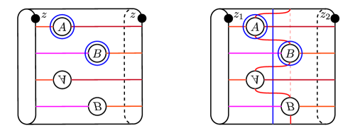
Figure 2. The tube-cutting piece. The diagram illustrates the genus $1$ case. Left: the standard bordered Heegaard diagram for the identity map of the torus. Right: the bordered Heegaard diagram $\mathsf{TC}$.

Theorem 12.

Let $\mathcal{H}$ be a bordered Heegaard diagram for an arced cobordism $Y$ from $F(\mathcal{Z})$ to itself. Let $T_{Y}$ denote the closed $3$-manifold obtained by gluing the two boundary components of $Y$ together in the obvious way, i.e.,

$$T_{Y}=Y/\bigl{(}F(\mathcal{Z})\ni x\sim x\in-F(\mathcal{Z})\bigr{)}.$$

Then

$$\mathit{HH}_{*}(\widehat{\mathit{BSDA}}(\mathcal{H}\mathbin{{}_{F(\mathcal{Z})}\mathord{\cup}_{-F(\mathcal{Z})}}\mathsf{TC}(\mathcal{Z})))\cong\widehat{\mathit{HF}}(T_{Y}).$$

Proof.

Let $\mathcal{H}^{\prime}$ be the sutured Heegaard diagram obtained by gluing $\mathcal{H}$ to the tube-cutting piece $\mathsf{TC}(\mathcal{Z})$ along both boundary components. From the self-pairing theorem for bordered-sutured Floer homology, Theorem 4.12,

$$H_{*}(\widehat{\mathit{BSA}}(\mathcal{H})\otimes^{L}_{\mathcal{A}(\mathcal{Z})\otimes\mathcal{A}(-\mathcal{Z})}\widehat{\mathit{BSD}}(\mathsf{TC}(\mathcal{Z}))=\mathit{SFH}(\mathcal{H}^{\prime}).$$

From the topological interpretation of $\mathsf{TC}(\mathcal{Z})$ and gluing properties of bordered-sutured diagrams [Zar09, Proposition 4.15], $\mathcal{H}^{\prime}$ is a sutured Heegaard diagram for $T_{Y}\setminus B^{3}$ with a single suture on the $S^{2}$ boundary component. Thus,

$$\mathit{SFH}(\mathcal{H}^{\prime})=\widehat{\mathit{HF}}(T_{Y})$$

(see [Juh06, Proposition 9.1]). ∎

We will also use a variant of the tube-cutting piece in order to prove that certain bimodules are neutral (Definition 3.17). Consider the Heegaard diagram $\mathsf{TC}(\mathcal{Z})$. Draw an arc $\gamma$ from $z_{1}$ to $z_{2}$ in $\Sigma\setminus(\alpha_{1}^{a}\cup\dots\cup\alpha_{2k}^{a}\cup\beta_{1}\cup\dots\cup\beta_{k}).$ Choose a point $z_{3}$ on $\gamma$, dividing $\gamma$ into two subarcs $\gamma_{13}$ from $z_{1}$ to $z_{3}$ and $\gamma_{32}$ from $z_{3}$ to $z_{2}$. Choose $z_{3}$ so that $\gamma_{13}$ intersects $\beta_{2k+1}$ once and is disjoint from $\alpha_{1}^{c}$, while $\gamma_{32}$ intersects $\alpha_{1}^{c}$ once and is disjoint from $\beta_{2k+1}$. (See Figure 3. It may be necessary to perturb $\alpha_{1}^{c}$, $\beta_{2k+1}$ and $\gamma$ in order to be able to choose $z_{3}$ this way.) Let

$$\mathsf{TC}_{0}(\mathcal{Z})=(\Sigma,\{\alpha_{1}^{a},\dots,\alpha_{2k}^{a},\alpha_{1}^{c}\},\{\beta_{1},\dots,\beta_{k},\beta_{k+1}\},\{z_{1},z_{2},z_{3}\}).$$

We can again view $\mathsf{TC}_{0}(\mathcal{Z})$ as a bordered-sutured Heegaard diagram, now representing $[0,1]\times F^{\circ}(\mathcal{Z})$ with sutures on $[0,1]\times(\partial F^{\circ}(\mathcal{Z}))$ as shown in Figure 3.

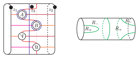
Figure 3. The diagram $\mathsf{TC}_{0}(\mathcal{Z})$ and the corresponding bordered-sutured manifold. Left: the genus $1$ case of the diagram $\mathsf{TC}_{0}(\mathcal{Z})$. Right: the corresponding sutures on $[0,1]\times S^{1}\subset\partial([0,1]\times F^{\circ}(\mathcal{Z}))$.

We are interested in $\mathsf{TC}_{0}(\mathcal{Z})$ because of two key properties. First:

Proposition 4.28.

The Heegaard diagram $\mathsf{TC}(\mathcal{Z})\cup_{\mathcal{Z}}\mathsf{TC}_{0}(\mathcal{Z})$ has trivial bordered-sutured invariants. In particular, $\widehat{\mathit{BSDA}}(\mathsf{TC}(\mathcal{Z}))\otimes^{L}_{\mathcal{A}(\mathcal{Z})}\widehat{\mathit{BSDA}}(\mathsf{TC}_{0}(\mathcal{Z}))$ is acyclic.

Proof.

One can perform a sequence of handleslides of the circle $\beta_{2k+1}$ in $\mathsf{TC}_{0}(\mathcal{Z})$ over other $\beta$-circles in $\mathsf{TC}(\mathcal{Z})\cup_{\mathcal{Z}}\mathsf{TC}_{0}(\mathcal{Z})$, followed by an isotopy, so that the resulting circle $\beta_{2k+1}^{\prime}$ is a small circle around $z_{3}$ disjoint from the $\alpha$-curves. Moreover, because of the placement of the basepoints, this diagram is still admissible. So, $\mathsf{TC}(\mathcal{Z})\cup_{\mathcal{Z}}\mathsf{TC}_{0}(\mathcal{Z})$ is equivalent to an admissible diagram in which there are no generators for the bordered-sutured invariants; this implies that the bordered-sutured invariants of $\mathsf{TC}(\mathcal{Z})\cup_{\mathcal{Z}}\mathsf{TC}_{0}(\mathcal{Z})$ are trivial. ∎

Let $\tau_{\partial}$ denote a positive Dehn twist of $F^{\circ}(\mathcal{Z})$ along a curve parallel to the boundary (“the boundary Dehn twist”) and $Y_{\tau_{\partial}}$ the mapping cylinder of $\tau_{\partial}$. Let $\tau_{\partial}^{-1}$ and $Y_{\tau_{\partial}^{-1}}$ denote the negative boundary Dehn twist and its mapping cylinder.

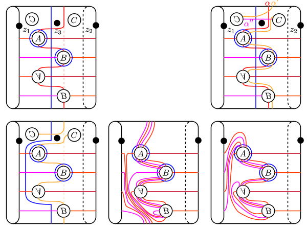
Figure 4. Exact triangle for $\mathsf{TC}_{0}(\mathcal{Z})$. Top left: the bordered-sutured Heegaard diagram $\mathsf{TC}_{0}(\mathcal{Z})$ with an extra handle. Top right: the bordered-sutured triple diagram inducing the exact triangle in Theorem 13. Bottom: Identifying the third term in the exact triangle with the positive boundary Dehn twist. The bottom left and bottom center differ by a sequence of handleslides and a destabilization; the bottom right is obtained by applying a surface diffeomorphism to the bottom center.

The second key property of $\mathsf{TC}_{0}(\mathcal{Z})$ is:

Theorem 13.

There are exact triangles

and

Proof.

We construct a bordered-sutured quadruple Heegaard diagram $(\Sigma,{\boldsymbol{\alpha}},{\boldsymbol{\alpha}}^{\prime},{\boldsymbol{\alpha}}^{\prime\prime},{\boldsymbol{\beta}},\{z_{1},z_{2},z_{3}\})$ with the following properties:

1. $\widehat{\mathit{BSDA}}(\Sigma,{\boldsymbol{\alpha}},{\boldsymbol{\beta}},\{z_{1},z_{2},z_{3}\})\cong\widehat{\mathit{BSDA}}(\mathsf{TC}_{0}(\mathcal{Z}))$. (In fact, the bordered-sutured 3-manifolds specified by $(\Sigma,{\boldsymbol{\alpha}},{\boldsymbol{\beta}},\{z_{1},z_{2},z_{3}\})$ and $\mathsf{TC}_{0}(\mathcal{Z})$ differ by a product decomposition.)

2. $(\Sigma,{\boldsymbol{\alpha}}^{\prime},{\boldsymbol{\beta}},\{z_{1},z_{2},z_{3}\})$ is a bordered-sutured Heegaard diagram for $\tau_{\partial}$.

3. $\widehat{\mathit{BSDA}}(\Sigma,{\boldsymbol{\alpha}}^{\prime\prime},{\boldsymbol{\beta}},\{z_{1},z_{2},z_{3}\})\simeq\mathcal{A}(\mathcal{Z})$. (In fact, $(\Sigma,{\boldsymbol{\alpha}}^{\prime\prime},{\boldsymbol{\beta}},\{z_{1},z_{2},z_{3}\})$ is a bordered Heegaard diagram for the mapping cylinder of the identity map.)

4. Each of ${\boldsymbol{\alpha}}$, ${\boldsymbol{\alpha}}^{\prime}$ and ${\boldsymbol{\alpha}}^{\prime\prime}$ consists of $2k$ arcs and $1$ circle.

5. The arcs in ${\boldsymbol{\alpha}}$, ${\boldsymbol{\alpha}}^{\prime}$ and ${\boldsymbol{\alpha}}^{\prime\prime}$ are the same.

6. Let $\alpha$, $\alpha^{\prime}$ and $\alpha^{\prime\prime}$ denote the circles in ${\boldsymbol{\alpha}}$, ${\boldsymbol{\alpha}}^{\prime}$ and ${\boldsymbol{\alpha}}^{\prime\prime}$, respectively. Then $\alpha$, $\alpha^{\prime}$ and $\alpha^{\prime\prime}$ all lie in a punctured torus $T$ in $\Sigma$ disjoint from the $\alpha$-arcs, and with respect to an appropriate orientation-preserving identification of $T$ with $\mathbb{R}^{2}/\mathbb{Z}^{2}$, $\alpha$ corresponds to the line $x=0$, $\alpha^{\prime}$ corresponds to the line $y=x$ and $\alpha^{\prime\prime}$ corresponds to the line $x=0$. (That is, $\alpha$, $\alpha^{\prime}$ and $\alpha^{\prime\prime}$ have slopes $\infty$, $1$ and $0$, respectively.)

The first exact triangle then follows from the pairing theorem in bordered-sutured Floer homology and the exact triangle of type $D$ invariants in [LOT08, Section 11.2]. (The strange cyclic ordering $\infty$–$1$–$0$ comes from the fact that we are varying the $\alpha$-circles, not the $\beta$-circles.)

The quadruple diagram is illustrated in Figure 4. To construct it, start with the bordered Heegaard diagram $\mathsf{TC}_{0}(\mathcal{Z})=(\Sigma^{\prime},{\boldsymbol{\alpha}},{\boldsymbol{\beta}},\{z_{1},z_{2},z_{3}\})$. Add a new handle with one foot near $z_{1}$ and one foot near $z_{3}$; call the resulting surface $\Sigma$. Since both feet of the new handle are in regions containing basepoints, $\widehat{\mathit{BSDA}}(\Sigma,{\boldsymbol{\alpha}},{\boldsymbol{\beta}},\{z_{1},z_{2},z_{3}\})\cong\widehat{\mathit{BSDA}}(\mathsf{TC}_{0}(\mathcal{Z}))$ (and, in fact, the corresponding bordered-sutured 3-manifolds differ by a disk decomposition).

Let $\alpha=\alpha_{1}^{c}$ be the unique circle in ${\boldsymbol{\alpha}}$. Let $\alpha^{\prime\prime}$ be a circle which runs along the new handle in $\Sigma$ once, intersects $\alpha$ and $\beta_{2k+1}$ once each, and is disjoint from the other $\alpha$- and $\beta$-curves. Obtain $\alpha^{\prime}$ from $\alpha^{\prime\prime}\cup\alpha$ by smoothing the unique crossing. There are two ways to perform this smoothing; one of the two gives curves satisfying property (6).

It remains to verify properties (2) and (3). Property (3) is easy: since the only $\beta$-circle that $\alpha^{\prime\prime}$ intersects is $\beta_{2k+1}$, any generator for $\widehat{\mathit{BSDA}}(\Sigma,{\boldsymbol{\alpha}}^{\prime},{\boldsymbol{\beta}},\{z_{1},z_{2},z_{3}\})$ must contain this point. This gives an identification of generators for $\widehat{\mathit{BSDA}}(\Sigma,{\boldsymbol{\alpha}}^{\prime},{\boldsymbol{\beta}},\{z_{1},z_{2},z_{3}\})$ and $\widehat{\mathit{BSDA}}$ of the standard Heegaard diagram for the identity cobordism. Moreover, the placement of the basepoints means that exactly the same curves are counted in the $A_{\infty}$-structure on the two bimodules. (Alternately, one can destabilize $\alpha^{\prime\prime}$ and $\beta_{2k+1}$ to obtain the standard Heegaard diagram for the identity cobordism.)

For Property (2), we manipulate the Heegaard diagram. Specifically, after performing a sequence of handleslides (two for each $\alpha$-arc on the left-hand side of the diagram, say) one can destabilize $\alpha^{\prime}$ and $\beta_{2k+1}$ to obtain a Heegaard diagram for the boundary Dehn twist; see Figure 4 for the genus $1$ case. (To be convinced of the sign of the Dehn twist, compare with [LOT11, Figure 12] and count the number of intersection points on each $\alpha$-arc.)

To obtain the second exact triangle, tensor the first with $\widehat{\mathit{BSDA}}(Y_{\tau_{\partial}^{-1}})$, and note that $\mathsf{TC}_{0}(\mathcal{Z})\cup_{F^{\circ}(\mathcal{Z})}Y_{\tau_{\partial}^{-1}}\cong\mathsf{TC}_{0}(\mathcal{Z})$. ∎

Corollary 4.29.

Let $f\nobreak\mskip 2.0mu\mathpunct{}\nonscript\mkern-3.0mu{:}\penalty 300\mskip 6.0mu plus 1.0mu\widehat{\mathit{BSDA}}(\tau_{\partial})\to\widehat{\mathit{BSDA}}(\mathbb{I})$ be the map from Theorem 13. Then the map

$$f\otimes\mathbb{I}\nobreak\mskip 2.0mu\mathpunct{}\nonscript\mkern-3.0mu{:}\penalty 300\mskip 6.0mu plus 1.0mu\widehat{\mathit{BSDA}}(Y_{\tau_{\partial}})\otimes^{L}\widehat{\mathit{BSDA}}(\mathsf{TC}(\mathcal{Z}))\to\widehat{\mathit{BSDA}}(\mathbb{I})\otimes^{L}\widehat{\mathit{BSDA}}(\mathsf{TC}(\mathcal{Z}))$$

is a quasi-isomorphism. In particular, for any $(\mathcal{A}(\mathcal{Z}),\mathcal{A}(\mathcal{Z}))$-bimodule $M$, $f$ induces an isomorphism

$$f_{*}\nobreak\mskip 2.0mu\mathpunct{}\nonscript\mkern-3.0mu{:}\penalty 300\mskip 6.0mu plus 1.0mu\mathit{HH}_{*}\bigl{(}\widehat{\mathit{BSDA}}(Y_{\tau_{\partial}})\otimes^{L}\widehat{\mathit{BSDA}}(\mathsf{TC}(\mathcal{Z}))\otimes^{L}M\bigr{)}\stackrel{{\scriptstyle\cong}}{{\longrightarrow}}\mathit{HH}_{*}\bigl{(}\widehat{\mathit{BSDA}}(\mathsf{TC}(\mathcal{Z}))\otimes^{L}M\bigr{)}$$

Proof.

Tensor the exact triangle in Theorem 13 with $\widehat{\mathit{BSDA}}(\mathsf{TC}(\mathcal{Z}))$ and apply Proposition 4.28 to see that every third term vanishes. ∎

Tensoring with the bimodule $\widehat{\mathit{BSDA}}(Y_{\tau_{\partial}^{-1}})$ is the Serre functor for the derived category of $\mathcal{A}(\mathcal{Z})$-bimodules [LOT11, Theorem 10]. In particular:

Theorem 4.30.

[LOT11, Corollary 11] For any $(\mathcal{A}(\mathcal{Z}),\mathcal{A}(\mathcal{Z}))$ bimodule $M$ we have

$$\mathit{HH}^{*}(M)\cong\mathit{HH}_{*}(\widehat{\mathit{BSDA}}(Y_{\tau_{\partial}})\otimes^{L}M).$$

Corollary 4.31.

Let $Y$ be a bordered-sutured $3$-manifold with bordered boundary $(-F^{\circ}(\mathcal{Z}))\amalg F^{\circ}(\mathcal{Z})$. Let $Y^{\prime}$ be the result of gluing $\mathsf{TC}(\mathcal{Z})$ to $Y$ along one boundary component. Then $\widehat{\mathit{BSDA}}(Y^{\prime})$ is a neutral bimodule.

Proof.

By Corollary 4.29, the map

$$f_{*}\nobreak\mskip 2.0mu\mathpunct{}\nonscript\mkern-3.0mu{:}\penalty 300\mskip 6.0mu plus 1.0mu\mathit{HH}_{*}(\widehat{\mathit{BSDA}}(Y_{\tau_{\partial}})\otimes^{L}\widehat{\mathit{BSDA}}(Y^{\prime}))\to\mathit{HH}_{*}(\widehat{\mathit{BSDA}}(Y^{\prime}))$$

is an isomorphism. By Theorem 4.30,

$$\mathit{HH}_{*}(\widehat{\mathit{BSDA}}(Y_{\tau_{\partial}})\otimes^{L}\widehat{\mathit{BSDA}}(Y^{\prime}))\cong\mathit{HH}^{*}(\widehat{\mathit{BSDA}}(Y^{\prime})).$$

It remains to see that the isomorphism $f_{*}$ is induced by an element of $\mathit{HH}_{*}(\mathcal{A}(\mathcal{Z}))$, i.e., a map $\mathcal{A}(\mathcal{Z})^{!}\to\mathcal{A}(\mathcal{Z})$. But by [LOT11, Proposition 5.13], $\widehat{\mathit{BSDA}}(Y_{\tau_{\partial}})\simeq\mathcal{A}(\mathcal{Z})^{!}$, so $f$ is indeed a map $\mathcal{A}(\mathcal{Z})^{!}\to\mathcal{A}(\mathcal{Z})$. ∎

Remark 4.32.

Theorem 13 can be seen as a special case of Honda’s bypass exact triangle (in the bordered-sutured setting). Proposition 4.28 can be deduced from the fact that a particular contact structure near $[0,1]\times\partial F^{\circ}(\mathcal{Z})$ is overtwisted.

4.5. Double covers of $3$-manifolds

We turn next to a rank inequality for a class of (unbranched) double covers. To spell out that class, recall that a double cover $\pi\nobreak\mskip 2.0mu\mathpunct{}\nonscript\mkern-3.0mu{:}\penalty 300\mskip 6.0mu plus 1.0mu\tilde{Y}\to Y$ corresponds to a homomorphism $p\nobreak\mskip 2.0mu\mathpunct{}\nonscript\mkern-3.0mu{:}\penalty 300\mskip 6.0mu plus 1.0mu\pi_{1}(Y)\to\mathbb{Z}/2$, which we can regard as an element $p\in H^{1}(Y,\mathbb{Z}/2)$. There is a canonical change-of-coefficient homomorphism $c\nobreak\mskip 2.0mu\mathpunct{}\nonscript\mkern-3.0mu{:}\penalty 300\mskip 6.0mu plus 1.0muH^{1}(Y,\mathbb{Z})\to H^{1}(Y,\mathbb{Z}/2)$.

Definition 4.33.

If $p$ is in the image of $c$ then we will say that $\pi$ is induced by a $\mathbb{Z}$-cover.

Lemma 4.34.

Let $Y$ be a closed $3$-manifold and let $\pi\nobreak\mskip 2.0mu\mathpunct{}\nonscript\mkern-3.0mu{:}\penalty 300\mskip 6.0mu plus 1.0mu\tilde{Y}\to Y$ be a $\mathbb{Z}/2$-cover induced by a $\mathbb{Z}$-cover. Then there is a bordered $3$-manifold $Y^{\prime}$ with two boundary components so that:

• $Y=T_{Y^{\prime}}$, the manifold obtained by gluing the boundary components of $Y^{\prime}$ together

• $\tilde{Y}=T_{Y^{\prime}\cup Y^{\prime}}$, the manifold obtained by gluing two copies of $Y^{\prime}$ together along their boundary, and

• the map $\pi$ is induced by the obvious map $Y^{\prime}\amalg Y^{\prime}\to Y^{\prime}$.

Proof.

With notation as above, suppose that $p=c(q)$. Since $S^{1}=K(\mathbb{Z},1)$, there is a map $f\nobreak\mskip 2.0mu\mathpunct{}\nonscript\mkern-3.0mu{:}\penalty 300\mskip 6.0mu plus 1.0muY\to S^{1}$ so that $q=f^{*}[S^{1}]$. Moreover, we may assume that $f$ is smooth and that $1\in S^{1}$ is a regular value of $f$. Then the manifold $Y^{\prime}$ obtained by cutting $Y$ along $f^{-1}(1)$ has the desired property. ∎

Proof of Theorem 3.

We will suppress the discussion of $\operatorname{spin}^{c}$-structures, which behave similarly to in Theorem 11.

Let $Y^{\prime}$ be as in Lemma 4.34 and let $\mathcal{H}$ be a bordered Heegaard diagram for $Y^{\prime}$, with boundary $-\mathcal{Z}\amalg\mathcal{Z}$. By Theorem 12,

$$\widehat{\mathit{HF}}(\tilde{Y})=\mathit{HH}_{*}(\widehat{\mathit{BSDA}}(\mathcal{H}\mathbin{{}_{F(\mathcal{Z})}\mathord{\cup}_{-F(\mathcal{Z})}}\mathsf{TC}(\mathcal{Z}))).$$

Let $\widetilde{\mathcal{H}}$ denote the result of gluing the boundary components of

$$\mathcal{H}\mathbin{{}_{F(\mathcal{Z})}\mathord{\cup}_{-F(\mathcal{Z})}}\mathsf{TC}(\mathcal{Z})\mathbin{{}_{F(\mathcal{Z})}\mathord{\cup}_{-F(\mathcal{Z})}}\mathcal{H}\mathbin{{}_{F(\mathcal{Z})}\mathord{\cup}_{-F(\mathcal{Z})}}\mathsf{TC}(\mathcal{Z})$$

together. On the one hand, the proof of Theorem 12 shows that

$$\mathit{HH}_{*}\bigl{(}\widehat{\mathit{BSDA}}(\mathcal{H}\mathbin{{}_{F(\mathcal{Z})}\mathord{\cup}_{-F(\mathcal{Z})}}\mathsf{TC}(\mathcal{Z})\mathbin{{}_{F(\mathcal{Z})}\mathord{\cup}_{-F(\mathcal{Z})}}\mathcal{H}\mathbin{{}_{F(\mathcal{Z})}\mathord{\cup}_{-F(\mathcal{Z})}}\mathsf{TC}(\mathcal{Z}))\bigr{)}\cong\mathit{SFH}(\widetilde{\mathcal{H}}).$$

On the other hand, from the topological interpretation of $\mathsf{TC}(\mathcal{Z})$, $\widetilde{\mathcal{H}}$ is a sutured Heegaard diagram for $\tilde{Y}\setminus(B^{3}\amalg B^{3})$, with one suture on each $S^{2}$ boundary component. So, by [Juh06, Proposition 9.14],

$$\mathit{SFH}(\widetilde{\mathcal{H}})\cong\widehat{\mathit{HF}}(\tilde{Y})\otimes H_{*}(S^{1}).$$

By Corollary 4.31, $\widehat{\mathit{BSDA}}(\mathcal{H}\mathbin{{}_{F(\mathcal{Z})}\mathord{\cup}_{-F(\mathcal{Z})}}\mathsf{TC}(\mathcal{Z}))$ is a neutral bimodule and so, by Corollary 4.26, $\widehat{\mathit{BSDA}}(\mathcal{H}\mathbin{{}_{F(\mathcal{Z})}\mathord{\cup}_{-F(\mathcal{Z})}}\mathsf{TC}(\mathcal{Z}))$ is $\pi$-formal. By Proposition 4.1, the bordered algebras are homologically smooth. So, the result follows from Theorem 4. ∎

References

- [CGH12a] Vincent Colin, Paolo Ghiggini, and Ko Honda, The equivalence of Heegaard Floer homology and embedded contact homology III: from hat to plus, 2012, arXiv:1208.1526.
- [CGH12b] by same author, The equivalence of Heegaard Floer homology and embedded contact homology via open book decompositions I, 2012, arXiv:1208.1074.
- [CGH12c] by same author, The equivalence of Heegaard Floer homology and embedded contact homology via open book decompositions II, 2012, arXiv:1208.1077.
- [DHK85] William Dwyer, Michael Hopkins, and Daniel Kan, The homotopy theory of cyclic sets, Trans. Amer. Math. Soc. 291 (1985), no. 1, 281–289.
- [Hen12] Kristen Hendricks, A rank inequality for the knot Floer homology of double branched covers, Algebr. Geom. Topol. 12 (2012), no. 4, 2127–2178, arXiv:1107.2154.
- [Juh06] András Juhász, Holomorphic discs and sutured manifolds, Algebr. Geom. Topol. 6 (2006), 1429–1457, arXiv:math/0601443.
- [Kal08] D. Kaledin, Non-commutative Hodge-to-de Rham degeneration via the method of Deligne-Illusie, Pure Appl. Math. Q. 4 (2008), no. 3, Special Issue: In honor of Fedor Bogomolov. Part 2, 785–875.
- [Kal09] Dmitry Kaledin, Cartier isomorphism and Hodge theory in the non-commutative case, Arithmetic geometry, Clay Math. Proc., vol. 8, Amer. Math. Soc., Providence, RI, 2009, pp. 537–562.
- [KLT10a] Çağatay Kutluhan, Yi-Jen Lee, and Clifford Henry Taubes, HF=HM I: Heegaard Floer homology and Seiberg–Witten Floer homology, 2010, arXiv:1007.1979.
- [KLT10b] by same author, HF=HM II: Reeb orbits and holomorphic curves for the ech/Heegaard-Floer correspondence, 2010, 1008.1595.
- [KLT10c] by same author, HF=HM III: Holomorphic curves and the differential for the ech/Heegaard Floer correspondence, 2010, arXiv:1010.3456.
- [KLT11] by same author, HF=HM IV: The Seiberg-Witten Floer homology and ech correspondence, 2011, arXiv:1107.2297.
- [KLT12] by same author, HF=HM V: Seiberg-Witten Floer homology and handle additions, 2012, arXiv:1204.0115.
- [Kon95] Maxim Kontsevich, Homological algebra of mirror symmetry, Proceedings of the International Congress of Mathematicians, Vol. 1, 2 (Zürich, 1994) (Basel), Birkhäuser, 1995, pp. 120–139.
- [KS09] M. Kontsevich and Y. Soibelman, Notes on -algebras, -categories and non-commutative geometry, Homological mirror symmetry, Lecture Notes in Phys., vol. 757, Springer, Berlin, 2009, arXiv:0606241v2, pp. 153–219.
- [Lod98] Jean-Louis Loday, Cyclic homology, second ed., Grundlehren der Mathematischen Wissenschaften [Fundamental Principles of Mathematical Sciences], vol. 301, Springer-Verlag, Berlin, 1998, Appendix E by María O. Ronco, Chapter 13 by the author in collaboration with Teimuraz Pirashvili.
- [LOT08] Robert Lipshitz, Peter S. Ozsváth, and Dylan P. Thurston, Bordered Heegaard Floer homology: Invariance and pairing, 2008, arXiv:0810.0687.
- [LOT10] by same author, Bimodules in bordered Heegaard Floer homology, 2010, arXiv:1003.0598.
- [LOT11] Robert Lipshitz, Peter S. Ozsváth, and Dylan P. Thurston, Heegaard Floer homology as morphism spaces, Quantum Topol. 2 (2011), no. 4, 381–449, arXiv:1005.1248.
- [LOT13] by same author, A faithful linear-categorical action of the mapping class group of a surface with boundary, J. Eur. Math. Soc. (JEMS) 15 (2013), no. 4, 1279–1307, arXiv:1012.1032.
- [LT12] Yi-Jen Lee and Clifford Henry Taubes, Periodic Floer homology and Seiberg-Witten-Floer cohomology, J. Symplectic Geom. 10 (2012), no. 1, 81–164, arXiv:0906.0383.
- [McC01] John McCleary, A user’s guide to spectral sequences, second ed., Cambridge Studies in Advanced Mathematics, vol. 58, Cambridge University Press, Cambridge, 2001.
- [OSz04] Peter S. Ozsváth and Zoltán Szabó, Holomorphic disks and knot invariants, Adv. Math. 186 (2004), no. 1, 58–116, arXiv:math.GT/0209056.
- [OSz08] by same author, Holomorphic disks, link invariants and the multi-variable Alexander polynomial, Algebr. Geom. Topol. 8 (2008), no. 2, 615–692, arXiv:math/0512286.
- [PP05] Alexander Polishchuk and Leonid Positselski, Quadratic algebras, University lecture series, vol. 37, American Mathematical Society, Providence, RI, 2005.
- [Ras03] Jacob Rasmussen, Floer homology and knot complements, Ph.D. thesis, Harvard University, Cambridge, MA, 2003, arXiv:math.GT/0306378.
- [Sei09] Paul Seidel, Symplectic homology as Hochschild homology, Algebraic geometry—Seattle 2005. Part 1, Proc. Sympos. Pure Math., vol. 80, Amer. Math. Soc., Providence, RI, 2009, pp. 415–434.
- [SS10] Paul Seidel and Ivan Smith, Localization for involutions in Floer cohomology, Geom. Funct. Anal. 20 (2010), no. 6, 1464–1501.
- [Tau10a] Clifford Henry Taubes, Embedded contact homology and Seiberg-Witten Floer cohomology I, Geom. Topol. 14 (2010), no. 5, 2497–2581.
- [Tau10b] by same author, Embedded contact homology and Seiberg-Witten Floer cohomology II, Geom. Topol. 14 (2010), no. 5, 2583–2720.
- [Tau10c] by same author, Embedded contact homology and Seiberg-Witten Floer cohomology III, Geom. Topol. 14 (2010), no. 5, 2721–2817.
- [Tau10d] by same author, Embedded contact homology and Seiberg-Witten Floer cohomology IV, Geom. Topol. 14 (2010), no. 5, 2819–2960.
- [Tau10e] by same author, Embedded contact homology and Seiberg-Witten Floer cohomology V, Geom. Topol. 14 (2010), no. 5, 2961–3000.
- [Zar09] Rumen Zarev, Bordered Floer homology for sutured manifolds, 2009, arXiv:0908.1106.