Optical interferometry in the presence of large phase diffusion
Abstract
Phase diffusion represents a crucial obstacle towards the implementation of high precision interferometric measurements and phase shift based communication channels. Here we present a nearly optimal interferometric scheme based on homodyne detection and coherent signals for the detection of a phase shift in the presence of large phase diffusion. In our scheme the ultimate bound to interferometric sensitivity is achieved already for a small number of measurements, of the order of hundreds, without using nonclassical light.
pacs:
07.60.Ly, 42.87.BgI Introduction
Optical interferometry represents a high accurate measurement scheme with wide applications in many fields of science and technology Cav81 ; r1 ; r2 ; r3 ; r4 . Besides, the precise estimation of an optical phase shift is relevant for optical communication schemes where information is encoded in the phase of travelling pulses. Several experimental protocols have been proposed and demonstrated to estimate the value of the optical phase Armen02 ; Mitch04 ; Nag07 ; Res07 ; Hig07 ; Hig09 and showing the possibility to attain the so-called Heisenberg limit Z92 ; Sam92 ; Lane93 ; San95 ; Eck06 ; Giov046 ; Guo08 ; Sme08 ; Gro11 ; Hay11 ; Bra11 . Recent developments also revealed the potential advantages of nonlinear interactions Boi08 . However, in realistic conditions, one has to retrieve phase information that has been unavoidably degraded by different sources of noise, which have to be taken into account in order to evaluate the interferometric precision Gio11 . The effects of imperfect photodetection in the measurement stage, or the presence of amplitude noise in the interferometric arms have been extensively studied Par95 ; Cam03 ; Huv08 ; Coo10 ; BanPhNat ; BanPhPRL ; Cab10 ; Joo11 ; DurkinPh ; Bah11 ; Dat11 . Only recently, the role of phase-diffusive noise in interferometry have been theoretically investigated for optical polarization qubit Bri10 ; Ber10 ; tes:11 , condensate systems BEC1 ; BEC2 , Bose-Josephson junctions Fer10 , and Gaussian states of light Gen11 . As a matter of fact, phase-diffusive noise is the most detrimental for interferometry and any signal that is unaffected by phase-diffusion, is also invariant under a phase shift, and thus totally useless for phase estimation.
In this paper, we present an experimental interferometric scheme where phase diffusion may be inserted in a controlled way, and demonstrate that homodyne detection and coherent signals are nearly optimal for the detection of a phase shift in the presence of large phase diffusion. Indeed, while in ideal conditions squeezed vacuum is the most sensitive Gaussian probe state for a given average photon number Mon06 , for large phase-diffusive noise, coherent states become the optimal choice, outperforming squeezed states Gen11 . In our scheme the ultimate bound to interferometric sensitivity, as dictated by the Cramér-Rao (CR) theorem, is achieved already for a small number of repeated measurements, of the order of hundreds, using Bayesian inference on homodyne data and without the need of nonclassical light.
The paper is structured as follows: In Section II we describe the evolution of a light beam in a phase diffusing environment as well as the bound to interferometric precision in the presence of phase noise. In Section III we describe our experimental apparatus, whereas the experimental results are reported and discussed in Section IV. Section V closes the paper with some concluding remarks.
II Interferometry in the presence of phase diffusion
The evolution of a light beam in a phase diffusing environment is described by the master equation
where and is the phase damping rate. An initial state evolves as
where , and . The diagonal elements are left unchanged, in fact energy is conserved, whereas the off-diagonal ones are progressively destroyed, together with the phase information carried by the state. Phase diffusion corresponds to the application of a random, zero-mean Gaussian-distributed phase shift, i.e.,
| (1) |
where is the phase shift operator.
We assume that the phase noise occurs between the application of the phase shift and the detection of the signal, and consider the estimation of a phase shift applied to a single-mode coherent state. Homodyne detection is then performed on the output state
and the value of the unknown phase shift is inferred using Bayesian estimation applied to homodyne data. Notice, however, that since the phase noise map and the phase shift operation commute, our results are valid also when the phase shift is applied to an already phase-diffused coherent state. The precision of the above procedure is then compared with the benchmarks given by i) the quantum CR bound for coherent states and any quantum limited kind of measurement, ii) the ultimate precision achievable with optimized Gaussian states, i.e., the quantum CR bound for general Gaussian signals, where, e.g., we allow for squeezing.
II.1 Interferometric precision in the presence of phase noise
The quantum CR bound Mal9X ; BC9X ; Bro9X ; LQE ; Dav11 is obtained starting from the Born rule where is the operator-valued measure describing the measurement and the density operator of the family of phase-shifted states under investigation. Upon introducing the (symmetric) logarithmic derivative as the operator satisfying
one proves that the ultimate limit to precision (independently on the measurement used) is given by the quantum CR bound
where is the quantum Fisher information (QFI). The ultimate sensitivity of an interferometer thus depends on the family of signals used to probe the phase shift and thus, as said above, we are going to compare the precision of our interferometer with the maximum achievable with coherent states, and with the ultimate precision achievable with optimized Gaussian states (for more details about the derivation of the corresponding quantum CR bounds see Gen11 ).
Homodyne detection measures the field quadrature
where is set to the optimal value to detect the imposed phase shift. The likelihood of a set of homodyne data
is the overall probability of the sample given the unknown phase , i.e.,
where
Assuming that no a priori information is available on the value of the phase shift (i.e., uniform prior), and using the Bayes theorem, one can write the a posteriori probability
| (2) |
being the parameter space. The probability is the expected distribution of given the data sample . The Bayesian estimator is the mean of the a posteriori distribution, whereas the sensitivity of the overall procedure corresponds to its variance
Bayesian estimators are known to be asymptotically unbiased and optimal, namely, they allow one to achieve the CR bound as the size of the data sample increases H9X ; O09 . On the other hand, the number of data needed to achieve the asymptotic region may depend on the specific implementation Bar00 . In the following we will experimentally show that our setup achieves optimal estimation already after collecting few hundreds of measurements.
III Experimental apparatus
A schematic diagram of the interferometer is reported in Fig. 1. The principal radiation source is provided by a He:Ne laser (12 mW, 633 nm) shot-noise limited above 2 MHz. The laser emits a linearly polarized beam in a TEM00 mode. The beam is splitted into two parts of variable relative intensity by a combination of a halfwave plate (HWP) and a polarizing beam splitter (PBS). The strongest part is sent directly to the homodyne detector where it acts as the local oscillator, whereas the ramaining part is used to encode the signal and will undergo the homodyne detection. The optical paths travelled by the local oscillator and the signal beams are carefully adjusted to obtain a visibility typically above 90% measured at one of the homodyne output ports. The signal is amplitude modulated at 4 MHz with a defined modulation depth to control the average number of photons in the generate state.
The amplitude modulation system consist of a KDP non-linear crystal with the axes at 45∘, and a PBS. The modulation is applied at the KDP crystal by means a waveform generator Rohde & Schwarz and a power amplifier Mini-Circuits ZHL-32A. The modulation depth is imposed at the proper level by a computer that sends a costant voltage to a mixer (M1) located between the waveform generator and the power amplifier. One of the mirrors in the signal path is piezo mounted to obtain a variable phase difference between the two beams. The piezo is preloaded and its resonance frequency is 13.5 kHz.
The phase difference is controlled by the computer after a calibration stage. The computer sends a voltage signal between 0 and 10 V that corresponds at the phase diffusion with a frequency of 5 kHz to a power amplifier based on LM675 integrated circuit that is able to drive the piezo at this frequency. With this system it is possibile to generate any kind of phase modulation.
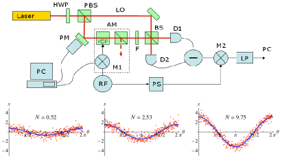
The detector is composed by a 50:50 beams splitter (BS) and a balanced amplifier detector with a bandwidth of 50 MHz. The difference photocurrent is filtered with high pass filters, amplified and demodulated at 4 MHz by means of an electrical mixer (M2). In this way the detection occurs outside any technical noise and, more importantly, in a spectral region where the laser does not carry excess noise. The signal is filterd by a low pass filter with a bandwidth of 300 kHz and sent to the computer through the National Instrument multichannel data acquisition 6251 with 16 bit of resolution and 1.25 MS/s sampling rate. The same device is used to send diffusion parameters to the phase modulator and signal parameters to the amplitude modulator.
IV Experimental results
In this Section, we present our experimental results, obtained with signals of different energies and different levels of noise. At first we show homodyne samples with the corresponding a posteriori distributions and then compare the precision obtained in our scheme with the ultimate bound imposed by the (quantum) Cramér-Rao theorem. Finally, we analyze the dependence of precision on the signal energy and the noise in order to illustrate how in the limit of large phase diffusion coherent states becomes the optimal Gaussian probe states. In fact, they outperform squeezed vacuum states, whose non-classical features are degraded by phase diffusion process, to an extent that make them useless for quantum metrology.
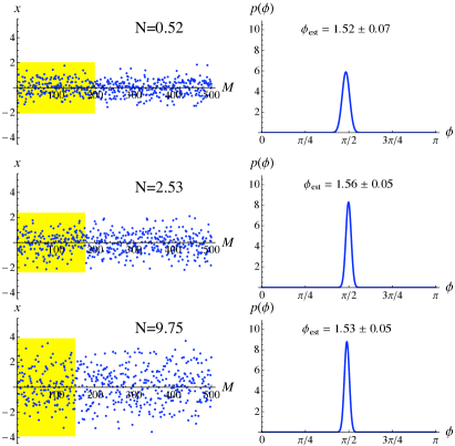
In Fig. 2 we report typical examples of homodyne samples, referred to a coherent signal with mean photon number measured at fixed optimal , together with the corresponding Bayesian a posteriori distribution for the phase shift. The yellow area denotes the portion of data used to infer the phase shift. We choose this range in order to emphasize that the optimality region in achieved already in that region. In fact, upon considering larger samples, precision would be improved, due to the statistical scaling of the variance , being a proportionality constant. On the other hand, optimality, i.e., the fact that
where is the QFI for phase-diffused coherent signals, is achieved for measurements. In the noiseless case the QFI is given by , whereas it decreases monotonically by increasing the value of the noise parameter . Notice that using optimized Gaussian signals, i.e. the squeezed vacuum state, one has a QFI given by in the noiseless case. However, in the presence of large phase diffusion, i.e. for large values of , is larger than the QFI obtained for phase-diffused squeezed vacuum states. In other words, coherent states turns out to be the optimal Gaussian probe states Gen11 .
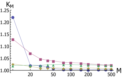
In Fig. 3 we plot the quantity
i.e., the variance of the Bayesian estimator from homodyne data multiplied by the number of data (measurements) and by the coherent states quantum Fisher information, as a function of . is by definition larger than one and expresses the ratio between the actual precision of the interferometric setup and the CR bound. As it is apparent from the plot rapidly decreases with the number of measurements, almost independently on the value of the number of photons and of the noise parameter . The optimality region, i.e., is achieved already for measurements, and the asymptotic value of is closer to 1 for increasing and . Furthermore, the number of measurements needed to achieve the optimal region may be (slightly) reduced by using the Jeffreys prior Jpp
instead of the uniform one, where
is the Fisher information of the homodyne distribution.
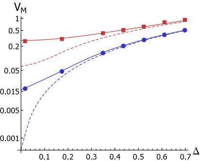
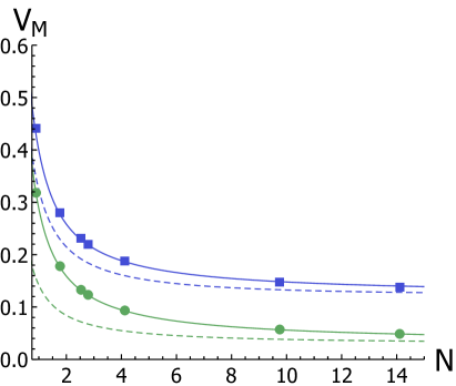
In Fig. 4 we show the variance of the Bayesian estimator from homodyne data
obtained after measurements, together with the CR bound for coherent states, and for the (phase-diffused) optimized Gaussian states, i.e., . In particular, the top panel shows the behaviour as a function of for different values of the number of photons , while in the bottom panel we plot the same quantities as a function of the number of photons and for different values of the noise . As it is apparent from the plots, nearly optimal inferferometric precision is achieved for increasing energy or phase diffusion, i.e., for larger values of or .
V Conclusions
In conclusion, we have demonstrated a nearly optimal interferometric scheme based on homodyne detection and coherent signals for the detection of a phase shift in the presence of large phase diffusion. Our scheme does not require nonclassical light and achieve the ultimate bound to interferometric sensitivity using Bayesian analysis on small samples of homodyne data, where the number of measurements is of the order of few hundreds.
It is worth noting that for large phase diffusion coherent states are the optimal Gaussian probe states. Indeed they outperform squeezed vacuum states, whose non-classical features are degraded by phase diffusion process, such that they become completely useless for quantum metrology.
Optical interferometry represents a high accurate measurement scheme with wide applications in many fields of science and technology, including high precision measurements and communication channels. On the other hand, phase diffusion represents a crucial obstacle towards the implementation of high precision interferometric measurements and phase shift based communication channels. Our results allow to design feasible, high-performance, communication channels also in the presence of phase noise, which cannot be effectively controlled in realistic conditions. Therefore, besides fundamental interest, our results also represent a benchmark for realistic phase based communication or measurement protocols.
Acknowledgements
This work has been supported by MIUR (FIRB “LiCHIS” - RBFR10YQ3H), the UK EPSRC (EP/I026436/1), MAE (INQUEST), UniMi (PUR2009 SIN.PHO.NANO), UIF/UFI (Vinci Program), and the University of Trieste (FRA2009).
References
- (1) C. M. Caves, Phys. Rev. D 23, 1693 (1981).
- (2) R. Bluhm, V. A. Kostelecky, C. D. Lane, N. Russel, Phys. Rev. Lett. 88, 090801 (2002).
- (3) C. Jentsch, T. Muller, E. Rasel, W. Ertmer, Gen. Rel. Gravit. 36, 2197 (2004).
- (4) S. Fray, C. A. Diez, T. W. Hänsch, M. Weitz, Phys. Rev. Lett. 93, 240404 (2004).
- (5) M. J. Snadden, J. M. NcGuirk, P. Bouyer, K. G. Haritos, M. A. Kasevich, Phys. Rev. Lett. 81, 971 (1998).
- (6) M. A. Armen, J. K. Au, J. K. Stockton, A. C. Doherty, and H. Mabuchi, Phys. Rev. Lett. 89, 133602 (2002).
- (7) M. W. Mitchell, J. S. Lundeen, and A. M. Steinberg, Nature 429, 161 (2004).
- (8) T. Nagata, R. Okamoto, J. L. O’Brien, K. Sasaki, and S. Takeuchi, Science 316, 726 (2007).
- (9) K. J. Resch, K. L. Pregnell, R. Prevedel, A. Gilchrist, G. J. Pryde, J. L. O’Brien, and A. G. White, Phys. Rev. Lett. 98, 223601 (2007).
- (10) B. L. Higgins, D. W. Berry, S. D. Bartlett, H. M. Wiseman, and G. J. Pryde, Nature 450, 393 (2007).
- (11) B. L. Higgins, D. W. Berry, S. D. Bartlett, M. W. Mitchell, H. M. Wiseman, and G. J. Pryde, New J. Phys. 11, 073023 (2009).
- (12) Z. Hradil Quantum Opt. 4, 93 (1992).
- (13) S. L. Braunstein, Phys. Rev. Lett. 69, 3598 (1992).
- (14) A. S. Lane, S. Braunstein, C. M. Caves, Phys. Rev. A 47, 1667 (1993).
- (15) B. C. Sanders, G. J. Milburn, Phys. Rev. Lett. 75, 2944 (1995).
- (16) K. Eckert, P. Hyllus, D. Bruss, U. V. Poulsen, M. Lewenstein, C. Jentsch, T. Muller, E. M. Rasel, W. Ertmer, Phys. Rev. A 73, 013814 (2006).
- (17) V. Giovannetti, S. Lloyd, and L. Maccone, Science 306, 1330 (2004); Phys. Rev. Lett. 96, 010401 (2006).
- (18) F. W. Sun, B. H. Liu, Y. X. Gong, Y. F. Huang, Z. Y. Ou, G. C. Guo, EPL 82, 24001 (2008).
- (19) L. Pezzé, A. Smerzi, G. Khoury, J.F. Hodelin, and D. Bouwmeester, Phys. Rev. Lett. 99, 223602 (2007); L. Pezzé, A. Smerzi, Phys. Rev. Lett. 100, 073601 (2008).
- (20) J. Grond, U. Hohenester, I. Mazets, and J. Schmiedmyer, New J. Phys. 12, 065036 (2010); J. Grond, U. Hohenester, J. Schmiedmayer, A. Smerzi, Phys. Rev. A 84, 023619 (2011).
- (21) M. Hayashi Progr. Inf. 8, 81 (2011).
- (22) D. Braun, J. Martin, Nat. Comm. 2, 223 (2011); D. Braun, Eur. Phys. J. D 59. 521 (2010).
- (23) S. Boixo, A. Datta, M. J. Davis, S. T. Flammia, A. Shaji, C. M. Caves, Phys. Rev. Lett. 101, 040403.
- (24) V. Giovannetti, S. Lloyd, and L. Maccone, Nat. Phot. 5, 222 (2011).
- (25) M. G. A. Paris, Phys. Lett A 201, 132 (1995); S. Olivares, M. G. A. Paris, Optics Spectr. 103, 231 (2007).
- (26) R. A. Campos, C. C. Gerry, and A. Benmoussa, Phys. Rev. A 68, 023810 (2003).
- (27) S. D. Huver, C. F. Wildfeuer, and J. P. Dowling, Phys. Rev. A 78, 063828 (2008).
- (28) J. J. Cooper, D. W. Hallwood, and J. A. Dunningham, Phys. Rev. A 81, 043624 (2010).
- (29) M. Kacprowicz, R. Demkowicz-Dobrzanski, W. Wasilewski, K. Banaszek, I. A. Walmsley, Nat. Phot. 4, 357 (2010).
- (30) U. Dorner, R. Demkowicz-Dobrzanski, B. J. Smith, J. S. Lundeen, W. Wasilewski, K. Banaszek and I. A. Walmsley, Phys. Rev. Lett. 102, 040403 (2009); Phys. Rev. A. 80, 013825 (2009).
- (31) H. Cable, G. A. Durkin, Phys. Rev. Lett. 105, 013603 (2010).
- (32) J. Joo, W. J. Munro, T. P. Spiller, Phys. Rev. Lett. 107, 083601 (2011).
- (33) S. Knysh, V. N. Smelyanskiy and G. A. Durkin, Phys. Rev. A 83, 021804(R) (2011).
- (34) T. B. Bahder, Phys. Rev. A 83, 053601 (2011).
- (35) A. Datta, L. Zhang, N. Thomas-Peter, U. Dorner, B. J. Smith, I. A. Walmsley, Phys. Rev. A 83, 063836 (2011).
- (36) D. Brivio, S. Cialdi, S. Vezzoli, B. Teklu, M. G. Genoni, S. Olivares, M. G. A. Paris, Phys. Rev. A 81, 012305 (2010).
- (37) B. Teklu, M. G. Genoni, S. Olivares, M. G. A. Paris, Phys. Scr. T140, 014062 (2010).
- (38) E. Tesio, S. Olivares and M. G. A. Paris, Int. J. Quant. Inf. 9, 379 (2011).
- (39) I. Tikhonenkov, M. G. Moore and A. Vardi, Phys. Rev. A 82, 043624 (2010).
- (40) Y. C. Liu, G. R. Jin, L. You, Phys. Rev. A 82, 045601 (2010).
- (41) G. Ferrini, D. Spehner, A. Minguzzi, F. W. J. Hekking, Phys. Rev. A 82, 033621 (2010).
- (42) M. G. Genoni, S. Olivares, M. G. A. Paris, Phys. Rev. Lett. 106, 153603 (2011).
- (43) A. Monras, Phys. Rev. A 73, 033821 (2006).
- (44) J. D. Malley, J. Hornstein, Stat. Sci. 8, 433 (1993).
- (45) S. L. Braunstein and C. M. Caves, Phys. Rev. Lett. 72, 3439 (1994); S. L. Braunstein, C. M. Caves and G. J. Milburn, Ann. Phys. 247, 135 (1996).
- (46) D. C. Brody, L. P. Hughston, Proc. Roy. Soc. Lond. A 454, 2445 (1998); A 455, 1683 (1999).
- (47) M. G. A. Paris, Int. J. Quant. Inf. 7, 125 (2009).
- (48) B. M. Escher, R. L. de Matos Filho, L. Davidovich, Nat. Phys. 7, 406 (2011); Braz. J. Phys. 41, 229 (2011).
- (49) Z. Hradil, Phys. Rev. A 51, 1875 (1995); Z. Hradil, R. Myška, and J. Peřina, M. Zawisky, Y. Hasegawa, H. Rauch, Phys. Rev. Lett. 76, 4295 (1996).
- (50) S. Olivares, M. G. A. Paris, J. Phys. B 42, 055506 (2009); B. Teklu, S. Olivares, M. G. A. Paris, J. Phys. B 42, 035502 (2009).
- (51) O. E. Barndorff-Nielsen and R. D. Gill, J. Phys. A 33, 4481 (2000).
- (52) H. Jeffreys, Proc. Roy. Soc. A 186, 453 (1946).