A Near-Infrared Template Derived from I Zw 1
for the Fe ii Emission in Active Galaxies

Abstract

In AGN spectra, a series of Fe ii multiplets form a pseudo-continuum that extends from the ultraviolet to the near-infrared (NIR). This emission is believed to originate in the Broad Line Region (BLR), and it has been known for a long time that pure photoionization fails to reproduce it in the most extreme cases, as does the collisional-excitation alone. The most recent models by Sigut & Pradhan (2003) include details of the Fe ii ion microphysics and cover a wide range in ionization parameter $\log U_{\rm ion}$= (-3.0 $\rightarrow$ -1.3) and density $\log n_{\rm H}$ = (9.6 $\rightarrow$ 12.6). With the aid of such models and a spectral synthesis approach, we study for the first time in detail the NIR emission of I Zw 1. The main goals are to confirm the role played by Ly$\alpha$ fluorescence mechanisms in the production of the Fe ii spectrum and to construct the first semi-empirical NIR Fe ii template that best represents this emission and can be used to subtract it in other sources. A good overall match between the observed Fe ii+Mg ii features with those predicted by the best fitted model is obtained, corroborating the Ly$\alpha$ fluorescence as a key process to understand the Fe ii spectrum. The best model is then adjusted by applying a deconvolution method on the observed Fe ii+Mg ii spectrum. The derived semi-empirical template is then fitted to the spectrum of Ark 564, suitably reproducing its observed Fe ii+Mg ii emission. Our approach extends the current set of available Fe ii templates into the NIR region.

1 Introduction

The broad-line region (BLR) of active galactic nuclei (AGN) is thought to consist of a roughly spherical mist of cloudlets with characteristic densities in the range 10⁹-10¹² cm^-3 and column densities of $\sim$10²⁴ cm^-2, surrouding a central source emitting ionizing radiation roughly isotropically (Sulentic et al., 2000; Gaskell, 2009). Despite the success of this traditional picture, in order to explain the strengths of the BLR lines, the need for a high covering factor and the lack of Lyman continuum absorption, a BLR having a flattened distribution at least for the low-ionization gas has been proposed (Gaskell, 2009).

The BLR has been extensively studied from the X-rays to the NIR regime during the last two decades (see the reviews of Sulentic et al., 2000; Gaskell, 2009). One of the most puzzling aspects of the line spectra emitted by the BLR is the Fe ii emission, whose numerous multiplets form a pseudo-continuum which extends from the UV to the optical region due to the blending of approximately 10⁵ lines. This emission constitutes one of the most important contributors to the cooling of the BLR.

Indeed, the blending of several BLR emission lines, including the large number of Fe ii emission multiplets, prevents a reliable study of individual line profiles and the identification and measurement of weaker lines. As blending is minimized in the class of objects known as Narrow-Line Seyfert 1 galaxies (NLS1s), their study can lead to a significantly more accurate study of the properties of the emission line region that is closer to the central source. Boroson & Green (1992), for instance, derived an optical template for the Fe ii multiplets from I Zw 1, which has served since then to adjust the Fe ii strength of several other objects, after a proper scaling and convolution to match the BLR velocity dispersions (estimated from strong emission lines). The advent of HST UV quasar spectral data allowed Vestergaard & Wilkes (2001) to extend the template method into the UV regime. They presented the first high S/N, high-resolution, quasar empirical UV iron template spectrum ranging from rest frame 1250 Å to 3090 Å, which is applicable to quasar data. The template was based on HST (archival) data of I Zw 1.

The iron emission templates have importance not only for our ability to measure and subtract the iron emission in quasar spectra, but also as a tool through which we can study the iron emission strength itself. Iron is a key coolant emitting $\sim$25% of the total energy output from the BLR (Wills, Netzer & Wills, 1985), emphasizing the importance of including the iron emission in studies of the BLR.

However, despite the wide use of such templates, most of the physical mechanisms that produce such lines remain under debate. There have been a number of pioneering theoretical investigations about the Fe ii emission spectra in active galactic nuclei (AGNs). For example, Phillips (1978a, 1978b) discussed continuum pumping as one of the excitation mechanisms that are responsible for that emission. Netzer & Wills (1983) and Wills, Netzer & Wills (1985) calculated the strengths of 3407 Fe ii emission lines assuming collisional excitation and continuum fluorescence of Fe ii, with radiative transfer in the spectral lines treated in the first-order escape probability approximation. They found a good fit to the overall shape of Fe ii features in the AGN UV and optical spectra but recognized that the total strength of the Fe ii emission is larger than the one predicted by the models by a factor of $\sim$4. Other attemps made by Collin-Souffrin et al. (1986) to solve the apparent weakness of the Fe ii emission using multi-component photoionization models were also unsuccessful. These failures point out that not all the excitation mechanisms have been taken into account or even that non-radiatively heated material with possibly even greater density exists within the BLR.

In order to solve the Fe ii problem, Penston (1987) suggested Ly$\alpha$ flourescence as the main physical process involved in the production of Fe ii lines. It takes advantage of the various near-coincidences between the wavelength of Ly$\alpha$ and the wavelengths corresponding to transitions between the levels of the $a^{4}D$ term and the $5p$ odd parity levels in Fe ii, as described by Johansson & Jordan (1984). The largest calculated transition probabilities from the odd $5p$ levels are those to $e^{4}D$ and $e^{6}D$, and cascades from these levels to odd parity levels at 5 eV and then to $a^{6}D$ and $a^{4}D$ would produce the bulk of the Fe ii spectrum located between 2000 Å  and 3000 Å.

Model calculations including Ly$\alpha$ fluorescence as the excitation mechanism for the Fe ii lines (Sigut & Pradhan, 1998, 2003) showed that this process is of fundamental importance in determining the strength of the Fe ii emission. Previously, Fe ii features in the intervals 2400-2560 Å  and 2830-2900 Å  that originate from high excitation levels ($\sim$10 eV) had been identified in the spectra of some AGNs (Graham, Clowes & Campusano, 1996; Laor et al., 1997), favouring the Ly$\alpha$ fluorescence scenario. The key feature to test this process, as predicted by Sigut & Pradhan (1998), is significant Fe ii emission in the wavelength range 8500-9500Å, where the primary cascade lines from the upper $5p$ levels to $e^{4}D$ and $e^{6}D$ are located. Up to a few years ago, that emission had been elusive to observe in AGNs although they are common features in the spectra of some Galactic sources (Hamman & Persson, 1989; Kelly, Rieke, & Campbell, 1994).

Fortunately, sensitive NIR spectroscopy carried out on AGN samples during the last decade at moderate spectral resolution (R$\sim$800) revealed a wealth of emission lines from Fe ii in a previously unexplored wavelength region. For instance, Rodríguez-Ardila et al. (2002), hereafter RA02, identified for the first time in four NLS1 galaxies (Ark 564, Mrk 335 (catalog MRK 0335), 1H 1934-063A (catalog 2MASX J19373299-0613046) and Mrk 1044 (catalog MRK 1044)) the strongest primary cascade lines of Ly$\alpha$ fluorescence predicted by Sigut & Pradhan (1998). In addition, the secondary UV lines resulting from the decay of the $e^{4}D$ and $e^{6}D$ levels are also present in these objects. Those results provided strong observational support to the hypothesis that Ly$\alpha$ fluorescence is, indeed, contributing to the emitted Fe ii spectrum. Furthermore, RA02 reports the presence of the so-called 1$\mu$m Fe ii lines (Fe ii $\lambda$9997, $\lambda$10501, $\lambda$10862 and $\lambda$11126). These are the most prominent Fe ii features observed in the rest wavelength interval 0.8-2.4 $\mu$m. The importance of that finding comes from the fact that nearly $\sim$50% of the optical Fe ii emission results from decays of the $z^{4}D^{0}$ and $z^{4}F^{0}$ levels, which are populated either by the transitions leading to the emission of the 1$\mu$m lines and the secondary UV lines mentioned above, or by collisions from lower levels and direct photoionization. Landt et al. (2008) reported similar findings in a sample of 23 well-known broad-emission line AGNs. They also confronted, for the first time, Sigut & Pradhan (1998) theoretical predictions of the NIR iron emission spectrum with observations. However, the prototypical I Zw 1 was not included in their sample.

The only observation to date of I Zw 1 in the NIR was reported by Rudy et al. (2000), hereafter RMPH. Their work clearly reveals Fe ii  $\lambda$9997, $\lambda$10501, $\lambda$10862, $\lambda$11126. Based on the absence of the crucial cascade lines that feed the common upper state where the 1 $\mu$m Fe ii lines originate (assuming Ly$\alpha$ fluorescence as the dominant mechanism) as well as the relatively low energy of that state, RMPH suggest that the observed lines are collisionally excited. Note, however, that no individual identification of the Fe ii lines in the 8500-9300 Å interval has yet been done in I Zw 1.

For all said above, I Zw 1 is a particularly good choice as a test target to construct a semi-empirical NIR Fe ii template as it is so well studied, especially in terms of its UV-optical iron emission. The strong and narrow Fe ii emission lines in I Zw 1, a conspicuous characteristic of NLS1 galaxies, make it an ideal object for the construction of such a template and complements the ones previously published in both the UV (Laor et al., 1997; Vestergaard & Wilkes, 2001) and in the optical region (Boroson & Green, 1992; Véron-Cetty, Joly & Véron, 2004).

Primary cascading lines following Ly$\alpha$ fluorescence, previously confirmed by RA02 and Landt et al. (2008) in other NLS1s, can also be studied and characterized in this source. The main 1 $\mu$m diagnostic lines have the advantage of not being heavily blended with other multiplets, as normally happens with the Fe ii optical lines. The observation of such features in I Zw 1 can serve as a useful benchmark for photoionization models, in particular, for models predicting the complex Fe ii emission spectrum. Moreover, the proposed semi-empirical Fe ii would allow the subtraction of this emission in other AGNs. This is important for at least two reasons: to decontaminate other BLR features and to evaluate the amount of Fe ii emission present in the NIR region, along with its relationship to that of the UV and optical region.

In this paper we describe the first detailed work to study the Fe ii lines emitted by the BLR in I Zw 1. The aim is twofold: (i) provide tight observational constraints to model the Fe ii emission in this source and (ii) construct the first semi-empirical template in the NIR region. The structure of this paper is as follows: Section 2 describes the observations and data reduction. Section 3 discusses the characteristics of the theoretical models used in this work. In Section 4 we perform a template fitting to the observed spectrum of I Zw 1, using the theoretical models described in the former section. Section 5 describes the construction of the semi-empirical Fe ii template and tests it on the NIR spectrum of Ark 564. A general discussion and conclusions are given in Sections 6 and 7, respectively.

2 Observations and Data Reduction

Near-infrared spectra of I Zw 1 were obtained at the NASA 3m Infrared Telescope Facility (IRTF) on the night of 23 October 2003. The SpeX spectrograph (Rayner et al. 2003) was used in the short cross- dispersed mode (SXD, 0.8 - 2.4 $\mu$m). The detector employed consisted of a 1024$\times$1024 ALADDIN 3 InSb array with a spatial scale of 0.15$\arcsec$/pixel. A $0.8\arcsec\times 15\arcsec$ slit oriented at the paralactic angle to minimize differential refraction was used, providing a spectral resolution of 360 km s^-1. This value was determined both from the arc lamp and the sky line spectra and was found to be constant with wavelength along the observed spectra.

During the observations the seeing was $\sim$1$\arcsec$ in J. Observations were done nodding in an ABBA pattern with integration time of 120 s per frame and total on-source integration time of 28 minutes. After the galaxy, the A0V star SAO 92128 (V=7.38) was observed as telluric standard and flux calibrator. The spectral reduction, extraction and wavelength calibration procedures were performed using SPEXTOOL (Cushing et al, 2004), the in-house software developed and provided by the SpeX team for the IRTF community. An aperture window 3$\arcsec$ wide was employed to integrate all the signal from the galaxy nucleus along the spatial direction. Extended emission is likely to be present but it is outside the 3$\arcsec$ region. Indeed, the FWHM of the I Zw 1 light profile matches, within the natural seeing fluctuations during the observations, that of the telluric standard (0.91$\arcsec$ for the former and 0.89$\arcsec$ for the latter in the $K$-band). The root-mean-square (RMS) of the dispersion solution for the wavelength calibration was 0.17Å.

The 1-D I Zw 1 spectrum was then corrected for telluric absorption and flux calibrated using Xtellcor (Vacca, Cushing & Rayner, 2003), another in-house software developed by the IRTF team. Finally, the different orders of the galaxy spectrum were merged to form a single 1-D frame. It was later corrected for the redshift of $z$=0.061105, determined from the average $z$ measured from the positions of Pa$\delta$, He i 1.083$\mu$m, Pa$\beta$ and Br$\gamma$. A Galactic extinction correction of E(B-V)=0.065 (Schlegel, Finkbeiner & Davis, 1998) was applied.

Figure 1 shows the final 1D spectrum of I Zw 1 already calibrated by wavelength and flux. A visual comparison of our SpeX data with that of RMPH reveals an improvement in the spectral resolution along the 0.8-2.2 $\mu$m, allowing us to better constrain most spectral features, in particular, those that are heavily blended. Moreover, the higher S/N ($\geq$150) of our spectrum eases the identification of new emission features not detected before. It can also be seen that the continuum flux scale is about 30% lower in the $z,J$ and$H$ band and 50% lower in the $K$ band than that of RMPH. This discrepancy is very likely due to the differences in apertures between the two observations, as our slit width is about 2.5$\times$ narrower, and therefore encompassing a much smaller contribution of the host galaxy. The minimum in the continuum emission, at $\sim$13000 Å  is characteristic of AGNs and is interpreted as due to a shift from a nonthermal continuum to the thermal dust emission that dominates at longer wavelengths (RMPH; RA02; Riffel, Rodríguez-Ardila & Pastoriza 2006; Landt et al. 2011). Note, however, that most line fluxes measured in our observation (see Table 2) agree within erros to that of RMPH.

Line identifications for the most conspicuous lines detected in the NIR spectrum of I Zw 1 are indicated in Figure 1.

It is easy to see from Figure 1 that the NIR spectrum of I Zw 1 is rich in Fe ii emission features. The so-called 1$\mu$m Fe ii lines, for instance, are particularly strong. Significant Fe ii emission in the 8500-9500 Å wavelength range, very likely produced by Ly$\alpha$ fluorescence as predicted by Sigut & Pradhan (1998), is also observed. Other prominent lines detected in I Zw 1 include H i, He i, O i and Ca ii. Moreover, forbidden lines of [Fe ii], and [S iii] and molecular H₂ were also detected.

In the following sections we will discuss the method employed for the construction of the first semi-empirical NIR Fe ii template published in the literature, suitable to remove this emission in AGNs after a proper subtraction of the continuum emission and scaling/ line broadening of the template.

3 The Fe ii models

Theoretical models of Fe ii including the NIR region are rare in the literature. Up to our knowledge, all works published before the year 1998 (Wills, Netzer & Wills 1985 and references therein) predicted emission line intensities for the UV and optical regions only. The main reason for ignoring the NIR is likely due to the fact that most model predictions pointed out to very weak Fe ii emission in that region. Moreover, the lack of good S/N observations of AGNs redwards of 8000 Å by that time prevented a confrontation between models and observations.

Sigut & Pradhan (1998) proposed that the inclusion of Ly$\alpha$ fluorescence excitation process results in significant NIR Fe ii emission in the region 8500-9500 Å. In these calculations, a limited, non-LTE atomic model with 262 fine structure levels, sufficiently large for Ly$\alpha$ fluorescent excitation, was included. They showed that Ly$\alpha$ excitation can be of fundamental importance in enhancing the UV and optical Fe ii fluxes.

Later, Sigut & Pradhan (2003) presented improved theoretical non-LTE Fe ii emission line strengths for physical conditions typical of active galactic nuclei with broad-line regions. In these new set of models, updated to also include the Mg ii ion (Sigut, 2004, private communication), the Fe ii line strengths were computed with a precise treatment of radiative transfer using extensive and accurate atomic data from the Iron Project (Sigut, Nahar & Pradhan, 2004). Excitation mechanisms for the Fe ii emission included continuum fluorescence, collisional excitation, self-fluorescence among the Fe ii transitions, and fluorescent excitation by Ly$\alpha$ and Ly$\beta$. A larger Fe ii atomic model consisting of 827 fine structure levels (including states to E$\sim$15 eV) was used to predict fluxes for approximately 23,000 Fe ii transitions, covering most of the UV, optical, and NIR wavelengths of astrophysical interest. Detailed radiative transfer in the lines, including self-fluorescence overlap, was perfomed with an approximate $\Lambda$ operator scheme - see Sigut & Pradhan (2003) for details.

Currently, owing to the complexity of the observed iron emission in AGNs, this emission is typically modeled using empirical templates derived from specific AGN spectra (Boroson & Green, 1992; Corbin & Boroson, 1996). A more recent example of application of this method consisted in deriving a Fe ii- iii template from high-quality UV spectra of the NLS1 galaxy I Zw 1 (Vestergaard & Wilkes, 2001). Such templates play a critical role in extracting a measure of the total iron emission from heavily blended and broadened AGN emission line spectra. Following this approach, and taking advantage of the availability of the Fe ii templates and the NIR spectrum of I Zw 1, we will construct the first semi-empirical Fe ii template of that galaxy, complementing the ones existing in the UV and optical regions. The approach that we will employ consists of comparing the NIR spectrum of I Zw 1 with a grid of Fe ii+Mg ii models developed by Sigut & Pradhan (2003), with these latter covering a wide range of ionization parameters ($U_{\rm ion}$=-1.3, -2 and -3 dex) and densities ($n_{\rm H}$ = 9.6, 10.6, 11.6 and 12.6 dex cm^-3). The internal cloud turbulent velocity, in all cases, was $V_{\rm tur}$=10 km s^-1. Fe ii+Mg ii spectra were computed for BLR cloud models with typical conditions thought to exist in the Fe ii emitting clouds. The calculations have been made for traditional clouds of a single specified density and ionization parameter, as opposed to the more realistic locally optimally emitting cloud models of Baldwin et al. (1995), as the main interest is to study the interplay of the various iron emission excitation mechanisms and not the detailed structure of the BLR.

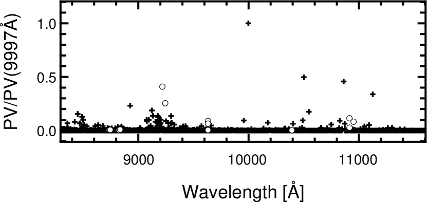
Figure 2: Peak-to-valley variability of the Fe ii+Mg ii models at each wavelength, normalized by its value at 9997 Å, for the 8300-11600 Å  region. Open circles refer to the Mg ii emission.

Figure 2 shows the peak-to-valley intensity variability among the Sigut & Pradhan models versus wavelength. It shows a rather large variation in strength in some emission lines, such as those contained in the 8300-8500 and 9000-9400 Å intervals (including a contribution from the Mg emission), Fe ii at 8927, 9997, 10502, 10862 and 11126 Å, as well as Mg ii at 9218 and 9244 Å. Indeed, the amplitude of the variation of these lines are about two orders of magnitude or more larger than the median peak-to-valley values.

4 Analysis Procedure

In order to estimate a NIR template for I Zw 1 a comparison of its observed emission line spectrum with that predicted by the available models was made. The best matching model can also indicate the most probable physical conditions of the BLR. As a by-product of the template fitting, we also determined the emission line positions/intensities of other BLR lines in order to minimize the residual RMS. The whole fitting procedure is decribed below.

The flux calibrated spectrum of I Zw 1 was first continuum-subtracted in order to leave us with a pure emission line spectrum. For this purpose, a spline function was fitted to the continuum, choosing regions free of emission lines. The $fit1d$ task of IRAF was used for this purpose, and chosen for simplicity. A more elaborate approach, consisting of a simultaneous fitting of the intrinsic AGN continuum, stellar population template and dust is out from the scope of this paper. Since the NIR spectrum is very rich in emission lines other than Fe ii, it is also necessary to model them and then perform a multi-parametric fit.

The Paschen series was modeled using, as a reference, the observed Pa$\alpha$ (1.8751 $\mu$m) profile in velocity space. In a first approach, we set the scaling factors of individual lines as free parameters in the fit. Pa$\beta$ is located in a region of strong telluric contamination and, for that reason, was not considered. Preliminary tests produced results without physical significance (i.e. not justifiable by internal reddening and/or deviations of case B recombination rates). For that reason, we decided to set limits on the relative intensities of such lines consistent with decreasing values as moving towards the bluer part of the spectrum, starting from Pa$\gamma$. This behavior was forced through the adoption of reasonable boundary conditions in the their scaling parameters. Moreover, Pa_i/Pa_i+1 line ratios in the 9000-12000 Å  range were allowed to have a 20-30% error, given the uncertainties in subtracting the continuum.

The permitted lines of Ca ii $\lambda$8498, $\lambda$8542, $\lambda$8662, He i $\lambda$10830, He ii $\lambda$10124 and O i $\lambda$8446, $\lambda$11287 are also generally blended with the iron multiplets. As the bulk of all these lines is produced by the BLR, they were also modeled through the Pa$\alpha$ profile, allowing some broadening (by up to 80 km s^-1 using Gaussian filtering) to improve the results. The centroid position of He i and He ii were found to be blueshifted by -332 and -622 km s^-1, respectively. This may indicate that the largest contribution of these two lines is produced in the NLR, in agreement with the results of Véron-Cetty, Joly & Véron (2004). They report two regions emitting broad and blueshifted [O iii] lines in the optical region. One of the systems has V=-500 km s^-1, compatible to the line shift of the helium lines found here. The other system has V=-1450 km s^-1. This latter is not detected here, very likely due to the lower spectral resolution of our data and its relative weakness compared to the strength of the other system. The fact that the iron line profiles do not appear asymmetric nor are significantly blueshifted indicates that this emission does not originate in the outflowing gas itself. This agrees with the results found by Vestergaard & Wilkes (2001).

Forbidden lines present in this spectral region such as [Ca i] $\lambda$9850 ($v_{r}\sim$213 km s^-1), the highly excited [S viii] $\lambda$9913 ($v_{r}\sim$-785 km s^-1), [S iii] $\lambda\lambda$9069,9532 (both with $v_{r}\sim$-300 km s^-1) and [S ii] $\lambda$10280, $\lambda$10320 have all been assumed to have Lorentzian profiles with widths of 600 km s^-1. The blue shift found in most of these lines are compatible with the shift found by Véron-Cetty, Joly & Véron (2004) in the optical spectrum, confirming the presence of a complex NLR in this object. We have fixed the FWHM of the forbidden lines because we verified that by progressively increasing their FWHM the residual RMS improved by clearly fitting through them also features of the Fe ii models, a not desirable effect. Also, the [S iii] doublet at 9069 and 9532 Å  were assumed to have their peak intensities constrained to the value of 2.4 ([S iii] $\lambda$9532/[S iii] $\lambda$9069), as determined by atomic physics. The list of all modeled emission lines is shown in table 1.

Our 12 available Fe ii+Mg ii (or simply the Fe ii, when not considering the Mg ii lines) theoretical templates had to be convolved with a line profile representative of the BLR. For that purpose, it is useful to examine Figure 3, where the Fe ii $\lambda$11126, O i $\lambda$11287 and Pa$\alpha$ emission line profiles are plotted in the velocity space. It is easy to see that all three profiles can be well represented by a Lorentzian function of FWHM = 875 km s^-1 (dashed curve). For comparison, the figure also shows a Gaussian profile (dotted) with the same FWHM as the Lorentzian. Clearly, the Gaussian fails at reproducing the extense wings observed in both lines. Because of the strong similarity of the BLR profiles with the Lorentzian curve, we adopted this theoretical profile to convolve our models. Notice that this system would be equivalent to the relatively broad L1 system of Véron-Cetty, Joly & Véron (2004), associated to the BLR.

Although it may sound appealing to use the form and width of Fe ii $\lambda$9997 or  $\lambda$10491+10502 to broaden the templates, note that the former is heavily blended with Pa$\delta$ (narrow and broad components), [S viii] and [C i], and the latter is a blend of two lines very close in wavelength. Therefore, the characterization of these profiles are more subject to uncertainties. As shown above, the form and width of either Fe ii $\lambda$11126 or O i $\lambda$11287 to broaden the Fe ii+Mg ii template provides a similar result. This is consistent also with previous works (Rodríguez-Ardila et al., 2002; Matsuoka et al., 2007) that presented consistent observational and theoretical evidence, respectively, that both Fe ii and O i are originated in the same parcel of gas.

Let each line intensity of a given Fe ii+Mg ii (or only Fe ii) template to be denoted by $l_{j}$ (a $\delta$-function at $\lambda_{j}$) and the Lorentzian velocity profile to be given by $P=P(v_{ij})$. The flux $f_{i}$ at a certain wavelenght $\lambda_{i}$ of the convolved template is then:

$$f_{i}\propto\sum_{all~{}j}l_{j}\times P(v_{ij})$$ (1)

with

$$v_{ij}=c~{}[(\lambda_{i}-\lambda_{j})/\lambda_{j}]$$

where $c$ is the speed of light. The proportionality constant on equation 1 is a parameter of the fit.

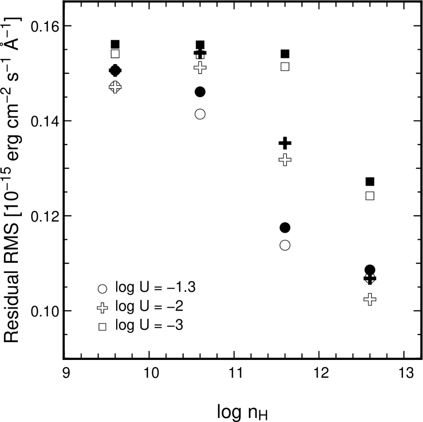
Figure 4: RMS of the residual spectrum of I Zw 1 after subtraction of fitted Fe ii+Mg ii models and emission lines, in the region between 8300 and 11600 Å. Solid symbols denote the results obtained using only the Fe ii multiplets (Mg ii neglected).

Once defined all the emission line profiles, we proceeded with the least-squares fit of all scaling parameters (19 in total for each model, correponding to the lines listed in Table 1 plus the convolved template scaling factor). This was carried out using the Fortran routines of the Minuit v. 94.1 software, available at the CERN library. The boundary conditions provided H i line ratios (Pa$\gamma$/Pa$\delta$, Pa$\delta$/Pa8, Pa8/Pa9, Pa9/Pa10) with an average of $\sim$1.7, consistent with the theoretical Paschen decrements within 20$-$30% error. Note that the reduced-$\chi^{2}$ provided by the routine does not take into account possible sources of errors such as residuals from telluric absorption corrections and continuum subtraction. For this reason, we used the RMS of the residuals as a measure for the quality of the fit. The residual RMS obtained from the fit of each of the 12 models, calculated in the the main region of interest (8300$-$11600 Å), is shown in Figure 4. These results are used as a discriminant of the best suitable model.

Models with medium/low ionization parameters and large densities such as (log $U_{\rm ion}$=-2.0, log $n_{\rm H}$=12.6) and (log $U_{\rm ion}$=-1.3, log $n_{\rm H}$=12.6) are the most successful ones, having residual RMS between 15-20% smaller with respect to the average (around 30% smaller considering the worst models). For consistency, we decided to check the effect of the Mg ii emission in the fits. For this purpose, we performed the same fitting procedure using only the Fe ii multiplets in the models. This approach is justified by the large uncertainties concerning the Mg ii strength in the models, specially in the spectral region of 9200 Å. The excitation mechanism for these Mg ii lines is Ly$\beta$ fluorescence, and the uncertainties come from the small transition probabilities between the levels 3s ²S $\rightarrow$ 5p ²P^o. Moreover, the pumping source function for Ly$\beta$ is more uncertain than for Ly$\alpha$ due to the fact that photons in Ly$\beta$ can also cycle through H$\alpha$, and this “cross-redistribution” can be important.

Considering that the number of Mg ii lines included in the Fe ii+Mg ii models is less than 1% of that of Fe ii, the exclusion of Mg ii does not affect significantly the fit, as expected. The RMS values of the fit residuals considering only the Fe ii multiplets are also shown in Figure 4 as solid symbols. The results are very similar to those obtained using the composite Fe ii+Mg ii models, favoring a high-density and moderate/low ionization parameter.

Another consistency check in the results was made considering only the 8300-11600 Å  region in the fit, where the main Fe ii diagnostic lines are located. In the above interval only Pa$\gamma$ to Pa10 were included in the fit, reducing the number of free parameters to 18. It turned out that either by fitting the larger 8300-20000 Å or just the 8300-11600 Å interval one obtains similar results. For this reason, and also because of the lack of significant Fe ii+Mg ii emission redwards of 11600 Å, we will concentrate in the remainder of this paper to this smaller spectral region.

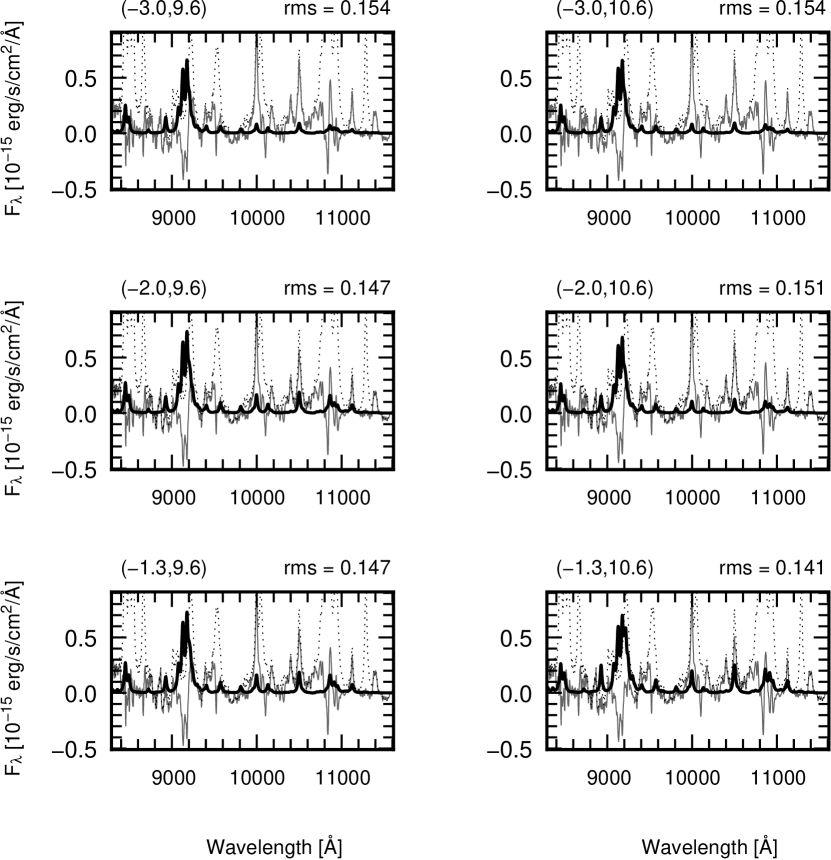
Figure 5: Results of the fitting procedure for the templates of Fe ii+Mg ii, for $\log n_{\rm H}$ of 9.6 and 10.6. Dotted lines are the continuum-subtracted spectrum of I Zw 1, solid-bold lines show the fitted (convolved) template, and the lighter solid lines are the fit residuals.

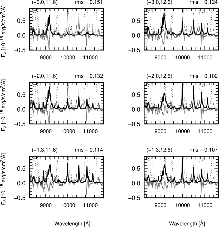
Figure 6: (Cont.): results of the fitting procedure for the templates of Fe ii+Mg ii, for $\log n_{\rm H}$ of 11.6 and 12.6. Dotted lines are the continuum-subtracted spectrum of I Zw 1, solid-bold lines show the fitted (convolved) template, and the lighter solid lines are the fit residuals.

Figures 5 and 6 show the best fits for all the models. Table 2 lists the emission line intensities derived from such fits.

5 Semi-empirical NIR Fe ii+Mg ii Template

In the previous section we found that the model with log $U$=-2 and log $n_{\rm H}$=12.6 is the one that best represents the observed Fe ii+Mg ii emission in I Zw 1. Although not crucial at this point, it is important to question if that model is consistent with the physical conditions of a Fe ii emission region believed to exist in AGNs.

Joly (1991) computed purely collisional models showing that low temperature ($T<$8000 K), high density ($n_{\rm H}>10^{11}~{}$cm^-3) and high column density ($N$(H)$>10^{22}$ cm^-2) clouds provide Fe ii${}_{\rm\,opt}$/H$\beta$ in good agreement with observations of Seyfert 1 galaxies. Detailed modeling of the Fe ii using Cloudy and including Ly$\alpha$ fluorescence as one of the excitation mechanisms made by Baldwin et al. (2004) points out to similar conditions. Indeed, densities between 9 $<~{}n_{\rm H}~{}<~{}13$ and log $U_{\rm ion}$=-1.4 are consistent with observations. Additional observational evidence that strong iron (Fe ii and Fe iii) emission may be connected with high densities was provided by Hartig & Baldwin (1986); Joly (1991); Baldwin et al. (1996); Lawrence et al. (1997) and Kuraszkiewicz et al. (2000). From that we can see that the physical conditions of the best matching model for I Zw 1 are, in general terms, representative of the Fe ii emitting region in AGNs.

In the remainder of this section we analyze in detail the best Fe ii+Mg ii template and propose modifications to it, based on the mismatches between the observed spectrum and the convolved model. We then present a semi-empirical template capable of minimizing the residual RMS in the NIR window of 8300-11600 Å  for I Zw 1.

The equation 1 for the convolution of a given model can be succinctly rewritten in a matricial form:

$$\boldsymbol{\mathit{f}}=\mbox{\bf P}~{}\boldsymbol{\ell}$$ (2)

where $\boldsymbol{\mathit{f}}$ denotes a spectrum, the N-length vector of Fe ii+Mg ii fluxes for a given wavelength range, P the N$\times$M convolution matrix and $\boldsymbol{\ell}$ the M-length vector with the set of Fe ii and Mg ii line intensities which contribute to the wavelength range comprised by $\boldsymbol{\mathit{f}}$. Neglecting any measurement errors, we can estimate $\boldsymbol{\mathit{f}}$ from the residuals of the observed spectrum after the subtraction of all emission lines (except Fe ii and Mg ii), which we call hereafter $\boldsymbol{\mathit{f}}_{obs}$. The convolution matrix can be easily built from the Lorentzian velocity profile (FWHM=875 km s^-1) and the $v_{ij}$ differences between each given multiplet line $l_{j}$ and the wavelength which corresponds to $f_{i}$. Adjusting the template line intensities to match as close as possible the observed residuals then constitutes a deconvolution problem, for which several solving approaches exist (see, for instance, a discussion on deconvolution techniques in Thièbaut 2005).

The number of Fe ii+Mg ii lines comprised between 8300 and 11600 Å  are 1529, out of which only a few contribute significantly to the emission spectrum. The Wiener deconvolution was chosen for our problem for its simplicity. However, it can lead to an unrealistic overdensity of line contributions, along with some unphysical results, if we consider all of the 1529 line intensities as free parameters. For this reason, we have decided to build a $\boldsymbol{\ell}^{*}$ vector containing only the contribution of multiplets with the $\approx$3% largest intensity contributions (selected from the best fitted model), plus some others whose intensities are clearly underestimated in the models (e.g. the unusual two-peaked bump around 11400 Å; see discussion below). In practice, this means zeroing the elements in the $\boldsymbol{\ell}$ vector (to be multiplied by P) which fall outside the selection criteria. The intensity threshold for building $\boldsymbol{\ell}^{*}$ lies at about 4% of the peak intensity in this wavelength range, and it is at least twice higher than the template median intensity. This criterium produces a $\boldsymbol{\ell}^{*}$ with 51 elements.

In order to account for the spectral contribution of the Fe ii+Mg ii multiplets not present in the $\boldsymbol{\ell}^{*}$ vector, which we call hereafter the “background” spectrum $\boldsymbol{\mathit{f}}_{b}$, we first subtract their emission from the input spectrum. This allows us to rewrite equation (2) as:

$$\boldsymbol{\mathit{f}}_{obs}^{*}=\boldsymbol{\mathit{f}}_{obs}-\boldsymbol{\mathit{f}}_{b}=\mbox{\bf P}~{}\boldsymbol{\ell}^{*}$$ (3)

Note that $\boldsymbol{\mathit{f}}_{b}$ is scaled accordingly to the fitted parameter of Fe ii+Mg ii found in the previous section. The line intensities in the vector $\boldsymbol{\ell}^{*}$ found from the deconvolution of $\boldsymbol{\mathit{f}}_{obs}^{*}$ plus the “background” subset of line intensities provide what we call the semi-empirical Fe ii+Mg ii template.

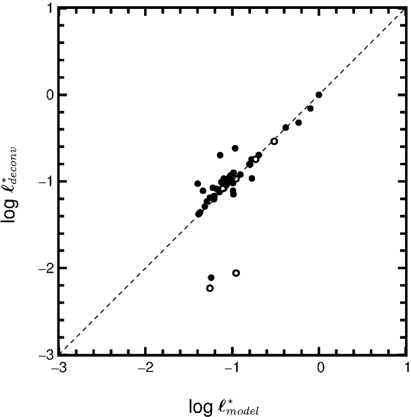
Figure 7: Comparison between the 51 elements of the input intensity vector $\boldsymbol{\ell}^{*}_{model}$ (=model) with those of the output one $\boldsymbol{\ell}^{*}_{deconv}$ (=deconvolved), normalized by the intensities at 9997Å. Filled and open circles denote Fe ii and Mg ii lines, respectively. The Wiener deconvolution gives a consistent result, specially for the strongest contributions. The dashed line represents the locus of the 1:1 relation.

A quick test used as $\boldsymbol{\mathit{f}}_{obs}$ a spectrum produced by convolving our best model, which we called $\boldsymbol{\mathit{f}}_{model}$. The deconvolution technique described above was then applied to check whether we could reliably recover the original $\boldsymbol{\ell}^{*}$, and consequently $\boldsymbol{\ell}$. Convolving this “deconvolved” vector then produced $\boldsymbol{\mathit{f}}_{deconv}$. The difference of this latter with $\boldsymbol{\mathit{f}}_{model}$ showed a RMS of less than 2% (relative to the intensity at 9997 Å). The reliability of this result is also shown in Figure 7, where the initial normalized model intensities ($\boldsymbol{\ell}^{*}_{model}$) are plotted against the ones found from the deconvolution ($\boldsymbol{\ell}^{*}_{deconv}$). Despite of some scattering, specially for the less intense lines, the agreement is very good.

When tackling real data, we decided to make a small tuning to the $\boldsymbol{\ell}^{*}$ vector. In order to conserve the physical interpretation given by the best model (-2.0,12.6) with predictions about the intensities of the most prominent Fe ii lines, we decided to discard them from the $\boldsymbol{\ell}^{*}$ vector. In practice this means that Fe ii $\lambda$9997, $\lambda$10501, $\lambda$10862,  $\lambda$11126 (and the close neighbors Fe ii $\lambda$10491, $\lambda$10871) had their original values preserved, and have been included in the $\boldsymbol{\mathit{f}}_{b}$ contribution. We should also make a brief remark on the relatively strong two-peaked bump of Fe ii observed at $\sim$11400 Å: this feature is underpredicted by any of the models, and because of its strength, we ruled out the possibility of being part of the spectrum noise or a feature introduced by the O i $\lambda$11287 profile fitting. Telluric absorption corrections are not critical in this region and, besides that, in the model templates one can notice two small peaks around this region, not exactly coincident in wavelength with the observed ones. These arguments give us support to believe that these features, located around 11381 and 11402 Å, are real. Notice that these wavelengths, estimated by visual inspection, are close to 11380.32 and 11403.54Å, which refer to features that appear in absorption in the models. We decided to include these two hypothetical lines in the $\boldsymbol{\ell}^{*}$ vector, as well as those around 10686 Å, clearly underestimated in the models but visible in $\boldsymbol{\mathit{f}}_{obs}^{*}$. This left us with a final 50-element $\boldsymbol{\ell}^{*}$ vector.

We then applied the deconvolution to the observed spectrum (after the $\boldsymbol{\mathit{f}}_{b}$ subtraction). The intensities obtained from the deconvolution method applied to the observed Fe ii+Mg ii I Zw 1 spectrum are shown in Table 3 together with those given by the best model. These values are all normalized with respect to the intensity of the Fe ii $\lambda$9997 line. For building the semi-empirical Fe ii+Mg ii spectrum we convolved this newly derived intensity vector with the P matrix and added back the background contribution.

The total semi-empirical template (corresponding to $\boldsymbol{\ell}$, according to our notation) in the region of interest (0.83-1.16 $\mu$m) is shown in Figure 8, on top. The bottom panel shows an expanded view ($\times$25) of the template, in order to highlight the contribution of the less intense lines.

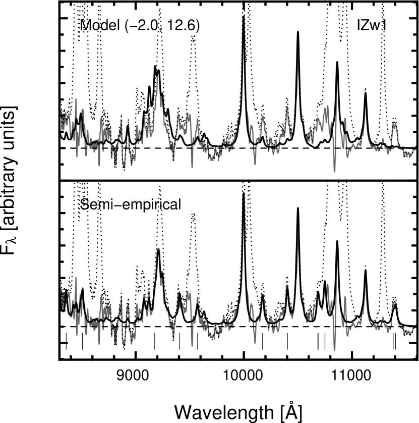
Figure 9: Top: Comparison of the observed Fe ii+Mg ii spectrum with the one derived from the best model (-2.0,12.9). Bottom: again the observed Fe ii+Mg ii spectrum, and the semi-empirical spectrum, computed through the template derived in this work. Dotted black line: total emission line spectrum of I Zw 1; solid grey and black lines: observed and model/semi-empirical Fe ii+Mg ii spectra, respectively. Dashed lines indicate the zero level intensity. Line intensities which varied significantly with respect to the model are also marked in the lower plot.

Figure 9 shows the resulting semi-empirical spectrum (bottom), as well as the one derived from best model (top), for comparison, superposed on the observed Fe ii+Mg ii spectrum of I Zw 1. The semi-empirical template reduces by $\sim$31% the RMS of the observed spectrum with respect to the best model. The bottom figure also indicates the lines whose estimated intensities varied more significantly with respect to those given by the model. Notice that negative intensities obtained from the deconvolution process have been zeroed in the computation of the estimated spectrum, but are shown in table 3 for completion. Such negative line intensities are consistent with zero within 2$\sigma$ of the spectral residuals.

Landt et al. (2008) [see their Section 5.4.1.] have compared the predicted Fe ii model of Sigut & Pradhan (2003) to observations and found a discrepancy in the the Fe ii 1.0491+1.0502 $\mu$m and Fe ii 1.0174 $\mu$m emission lines, in the sense that the former were overpredicted whereas the latter were underpredicted by theory, and this by a similar factor of $\sim$2. Note that they used the predictions of model A of Sigut & Pradhan (2003) with log $U_{\rm ion}$=-2 and log $n_{\rm H}$=9.6. Our best matching model has the same ionization parameter but a density that is three orders of magnitude larger (log $n_{\rm H}$=12.6). As can be seen in Table 2 and Figures 5 and 6, our best model leads to a better fit of the most conspicuous lines including Fe ii 1.0491+1.0502 $\mu$m. Indeed, the discrepancy is removed in this pair of emission lines. Fe ii 1.0174 $\mu$m, on the other hand, continues to be underpredicted even in the best model. Actually, this was one of the iron features that needed a fine tuning: its strength increased in the semi-empirical template by a factor of almost 3 (see Figure 11, when a comparison between the model and the semi-empirical template is done). Very likely, atomic parameters for that line would need to be reviewed in future modeling.

5.1 Application to Ark 564

Ark 564 is another well-known NLS1 with strong Fe ii emission, suitable to test our semi-empirical template. The spectrum of this AGN was observed and reduced in a similar way to that of of I Zw 1. Details of the extraction, reduction, wavelength and flux calibration are in Rodríguez-Ardila et al. (2004). As previously, we fitted and subtracted the continuum emission through a spline function. For modeling the line profiles, we adopted Pa$\alpha$ as representative of the emission line profile to be convolved with the Fe ii+Mg ii intensity vector derived from I Zw 1, and also as a template for other permitted emission lines. Forbidden lines were assumed to have Gaussian profiles with widths of 500-550 km s^-1. A quick fit over all the theoretical models also indicates a very high density and low/moderate ionization parameter for the Fe ii emitting region, as shown in Table 4 with the estimated RMS over the 8300-11600 Å  region. The sharpness of the emission lines makes small uncertainties in emission line positioning and scaling to give rise to high amplitude residuals in the fit, what explains the larger observed residual RMS. Neverthless, the general trend is similar to that observed for I Zw 1, favoring similar physical conditions for the Fe ii emitting region.

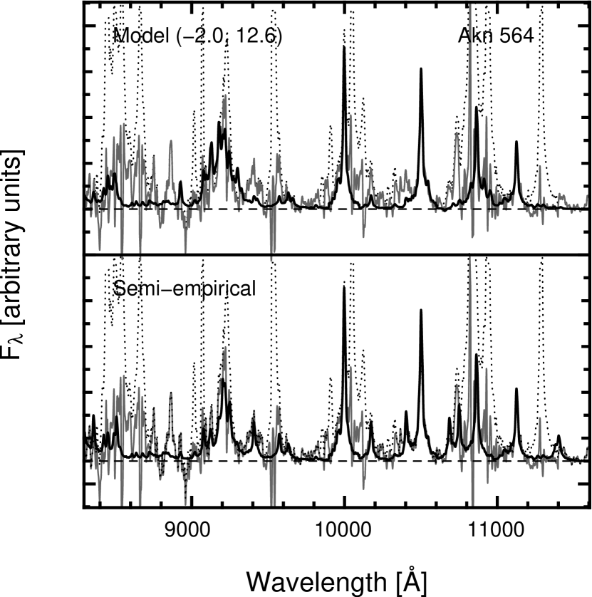
Figure 10: Top: Comparison of the observed Fe ii+Mg ii spectrum of Ark 564 with the one derived from the best model (-2.0,12.9). Bottom: again the observed Fe ii+Mg ii spectrum, and the semi-empirical spectrum, computed through the template derived from I Zw 1. Dotted black line: total emission line spectrum of Ark 564; solid grey and black lines: observed and model/semi-empirical FeII+MgII spectra, respectively. Dashed lines: zero intensity level.

Figure 10 is similar to figure 9, but now showing the suitability of our derived semi-empirical template to the observed Fe ii+Mg ii emission of Ark 564. A smaller RMS in the residuals with respect to those obtained from the theoretical models confirms the usefulness of the semi-empirical template to represent the Fe ii and Mg ii emission in AGNs. In general, lines that needed a fine tuning in I Zw 1, like Fe ii 10174 Å, properly reproduce the observations. Note, however, that the bump observed at 11400 Å in I Zw 1 and that we deliberately introduced in the template seems to be unusually large with respect to the one in Ark 564. Clearly, the transitions leading to these particular set of lines should strongly depend on local physical parameters that vary from object to object.

6 Discussion

The analysis carried out in the previous sections confirms several pieces of evidence already suggested by other works, which are: (i) Ly$\alpha$ fluorescence is indeed a process that should be taken into account in any systematic study of the Fe ii emission in AGNs as it produces a considerable amount of emission lines that otherwise would be absent. This is particularly evident for the 9200 Å feature, composed of numerous Fe ii multiples as well as some contribution from Mg ii lines. (ii) Similarly to the optical region, the NIR Fe ii emission also produces a subtle pseudo-continuum, particularly in the region between 8600 and 10000 Å (see Figure 8). Without a proper modeling and subtraction of this emission, fluxes of other BLR and NLR features can be severely overestimated. (3) Unlike in the optical region, individual Fe ii emission lines can be isolated in the NIR (i.e., the lines at 10501 Å, 10862 Å and 11126 Å). This is particularly useful to characterize, for instance, the line profiles and emission line fluxes, in an already complex emission region. This individual Fe ii line charaterization can be possible because other Fe ii lines very close in wavelength to the above three are at least 25$\times$ weaker.

The above thoughts can better be visualized in Figure 11, which shows the spectrum of I Zw 1 with (top) and without (bottom) the Fe ii+Mg ii contribution. The spectrum “clean” of iron and magnesium emission highlights the remaining emission lines, properly identified in the figure. Small spikes, coincident with the position of the strongest Fe ii lines can still be seen as, for example, in the blue part of Pa$\delta$, between He i and Pa$\gamma$ and at the position of the Fe ii $\lambda$11126 line. We interpret these small residuals as a due to emission from the NLR, as suggested by Véron-Cetty, Joly & Véron (2004). It might indicate that a more complex modeling of the convolving profile might be required, for example, by including a possible contribution from the NLR. However, because we are primarily interested in the construction of a semi-empirical template for the Fe ii+Mg ii emission which originates at the BLR, these small residuals are out of concern.

Figure 12 shows the same as figure 11 but for Ark 564. It can be seen that the spectrum at the bottom is nicely clean of Fe ii and Mg ii, as evidenced by the small residuals left in the region between 10200-10600 Å. It exemplifies the use of our NIR I Zw 1 template to remove that emission in other AGNs.

At this point we call the attention to an apparent absorption feature blueward of He i $\lambda$10818 that appeared after the subtraction of the Fe ii+Mg ii semi-empirical template in Ark 564. It is possible that this feature is artificial and due to a bad subtraction of the Fe ii blends with peak at 10750 Å. Yet another possibility is that it could be a real feature, similar to the one reported by Leighly, Dietrich, & Barber (2011) in the quasar FBQSJ1151+3822 (catalog FBQS J1151+3822), which they attribute to a broad absorption line (BAL) system in that source. Leighly, Dietrich, & Barber (2011) discussed the prospects of finding other He i $\lambda$10830 BALQSOs on six additional objects and pointed out that several well-known, bright low-redshift BALQSOs have no He i $\lambda$10830 absorption, a fact that can place upper limits on the column densities in those objects. Observations with higher spectral resolution are needed to confirm if the absorption in Ark 564 is indeed real. Although it is out of the scope of this paper the study of such a system of absorbers in the BLR of Ark 564 or in other sources, our results strengthen the need of an adequate Fe ii subtraction around He i $\lambda$10830 to further constrain the inner physical properties of such AGNs.

Note also that the peak observed around 10740 Å  is due to [Fe xiii] emission. In addition, the 11400 Å bump is overestimated in the semi-empirical template, meaning that some particular lines may need a fine tuning for a better match. It implies also that not all NIR Fe ii lines may scale up by the same factor, as would be expected. However, as in the optical and UV regions, the semi-empirical template suitably reproduces most of the observed Fe ii+Mg ii emission features in the NIR. Clearly, testing the template in a large number of objects is necessary to verify its suitability in more general terms.

At this point is important to draw our attention to how significant is the NIR Fe ii emission in I Zw 1 compared to that of the optical and UV. For this purpose we measured the integrated flux in the 8300$-$11600 Å region using the Fe ii semi-empirical template derived for that object. We found that F${}_{Fe\,{\sc II}}=2.79\pm 0.20\times 10^{-13}$ erg cm^-2 s^-1. Note that the Mg ii was not taken into account in the computed value. Tsuzuki et al. (2006) measured the integrated flux of Fe ii for I Zw 1 using HST and ground-based observations of this galaxy in five different wavelength bands: $U$1 [2200-2660 Å], $U$2 [2660-3000 Å], $U$3 [3000-3500 Å], $O$1 [4400-4700 Å] and $O$2 [5100-5600 Å]. The values they found, relative to H$\beta$, are shown in Table 5.

It can be seen that nearly half the amount of H$\beta$ flux in I Zw 1 is emitted by Fe ii in the NIR. Moreover, the integrated NIR iron emission carries a flux that is equivalent to $\sim$10% of the Fe ii emission in the optical region (sum of the fluxes in the $O$1 and $O$2 intervals of Table 5), to $\sim$10% of the Fe ii in the near-UV region (3000-3500 Å) and to $\sim$3% of the Fe ii emission in the UV (2200-3000 Å).

At first sight the above numbers may indicate that the role of Ly$\alpha$ pumping, which is behind most of the Fe ii NIR emission, is negligible. However, we should take into account that after the cascading transitions that result in the NIR emission the z ⁴D and z ⁴F levels are populated. These latter are responsible for part of the transitions leading to the Fe ii emission in the $O$1 and $O$2 optical regions. Therefore, a 10% in flux means that up to 20% of the optical Fe ii photons can be attributed to Ly$\alpha$ fluorescence.

7 Conclusions

We have compared theoretical models for the Fe ii+Mg ii NIR emission in active galaxies, which have the same turbulent velocities in the medium, but differ in physical conditions such as density and degree of ionization of the emitting region. For that purpose, we chose to model the NLS1 galaxy I Zw 1, which has traditionally provided the template for the Fe ii emission in the optical and UV.

The best match among all models was obtained by comparing the results of a multi-parametric fit comprising the main emission line features to the observed spectrum in the region 0.83-1.16 $\mu$m. Low/moderate ionization parameters and high gas densities of 10^12.6 cm^-3) are favored, as they reduce the residuals of the fitted spectrum. However, since some Fe ii lines are clearly underestimated even by the best models, we decided to derive a semi-empirical template to improve the fitting, by adjusting the intensities of the most prominent Fe ii and Mg ii lines, taken from the best fitted model.

The newly derived template reduces the fit residuals by about 31% with respect to what is obtained using the best theoretical model. We performed a quick check on the spectrum of another NLS1 with conspicuous and very narrow emission lines, Ark 564. Despite some small differences, this test corroborated the reliability of this new semi-empirical template to reproduce AGN Fe ii and Mg ii emission lines in the NIR.

We also highlight that the Fe ii bump around 11400 Å which we introduced to match the observed spectrum of I Zw 1 does not reproduce well the same observed feature of Ark 564. This lead us to the conclusion that this emission is abnormal in I Zw 1, given that none of the models too could predict such a large emission. Also, I Zw 1 might contain a narrow contribution to the Fe ii spectrum, as suggested in an optical study of Véron-Cetty, Joly & Véron (2004). Further tests will be futurely carried out on a larger sample, in order to fine tune our derived template.

Table 1: Template lines that were added to the Fe ii+Mg ii fitting process.

Line	$\lambda_{rest}$ (Å)	$\lambda_{meas}$ (Å)	Profile
Pa$\alpha$	18750	18750	itself
Pa$\gamma$	10937	10937	Pa$\alpha$
Pa$\delta$	10049	10049	Pa$\alpha$
Pa8	9544	9544	Pa$\alpha$
Pa9	9230	9230	Pa$\alpha$
Pa10	9014	9014	Pa$\alpha$
Ca ii	8498	8498	Pa$\alpha$
Ca ii	8542	8542	Pa$\alpha$
Ca ii	8662	8662	Pa$\alpha$
O i	8446	8446	OI$\lambda$11287
O i	11287	11287	OI$\lambda$11287
He i	10830	10818	Pa$\alpha$
He ii	10124	10103	Pa$\alpha$
$[$CaI$]$	9850	9857	Lorentzian
$[$S ii$]$	10280	10280	Lorentzian
$[$S ii$]$	10320	10320	Lorentzian
$[$S iii$]$	9069	9060	Lorentzian
$[$S iii$]$	9532	9521	Lorentzian
$[$S viii$]$	9913	9888	Lorentzian

Table 2: Fluxes of I Zw 1 emission lines obtained from the fitting of Fe ii+Mg ii (in units of 10^-14 erg s^-1 cm^-2).

	log $U_{\rm ion}$=-3				log $U_{\rm ion}$=-2				log $U_{\rm ion}$=-1.3
log $n_{\rm H}$	9.6	10.6	11.6	12.6	9.6	10.6	11.6	12.6	9.6	10.6	11.6	12.6
Pa$\gamma$ (10937Å)	9.18	9.16	9.01	8.64	8.81	8.96	8.64	8.64	8.82	8.64	8.64	8.64
Pa$\delta$ (10049Å)	4.41	4.41	4.41	4.41	4.41	4.41	4.41	4.41	4.41	4.41	4.41	4.41
Pa8 (9544Å)	2.78	2.78	2.78	2.78	2.78	2.78	2.78	2.78	2.78	2.78	2.78	2.78
Pa9 (9230Å)	2.22	2.22	2.22	2.22	2.22	2.22	2.22	2.22	2.22	2.22	2.17	2.17
Pa10 (9014Å)	1.43	1.43	1.39	1.26	1.38	1.40	1.26	1.24	1.38	1.32	1.17	1.12
He i (10830Å)	18.9	18.9	18.7	17.8	18.6	18.8	18.0	17.3	18.7	18.4	17.3	17.4
He ii (10124Å)	1.73	1.73	1.75	1.59	1.61	1.73	1.63	1.39	1.63	1.67	1.49	1.40
O i (8446Å)	7.21	7.21	7.15	7.03	7.14	7.17	7.04	7.30	7.14	7.15	7.28	7.30
O i (11287Å)	4.62	4.63	4.62	4.52	4.60	4.62	4.55	4.47	4.62	4.58	4.50	4.44
Ca ii (8498Å)	3.63	3.62	3.54	3.06	3.57	3.57	3.21	3.09	3.56	3.45	3.19	3.00
Ca ii (8542Å)	5.93	5.93	5.92	5.86	5.92	5.92	5.88	5.79	5.92	5.90	5.83	5.75
Ca ii (8662Å)	5.19	5.19	5.18	5.10	5.17	5.18	5.12	4.95	5.17	5.16	5.04	4.83
$[$Ca i$]$ (9850Å)	0.25	0.25	0.25	0.24	0.24	0.25	0.24	0.22	0.24	0.24	0.23	0.23
$[$S ii$]$ (10280+10320Å)	1.00	1.00	0.99	0.87	0.98	1.00	0.91	0.79	0.99	0.96	0.84	0.84
$[$S iii$]$ (9530+9068Å)	3.03	3.03	2.99	2.85	2.96	2.99	2.86	2.89	2.96	2.93	2.88	2.83
$[$S viii$]$ (9913Å)	0.51	0.51	0.50	0.43	0.49	0.50	0.45	0.35	0.49	0.48	0.39	0.35
Fe ii (9997Å)	0.34	0.34	0.45	1.99	0.69	0.45	1.49	3.78	0.68	0.84	2.77	3.73
Fe ii (10501Å)	0.35	0.36	0.50	2.06	0.74	0.49	1.68	3.16	0.74	0.99	2.37	1.94
Fe ii (10863Å)	0.28	0.31	0.43	1.69	0.65	0.42	1.43	2.41	0.67	0.85	2.33	1.86
Fe ii (11126Å)	0.14	0.16	0.25	1.11	0.33	0.23	0.89	1.70	0.34	0.49	1.51	1.37
Fe ii (9000-9400Å)	6.37	6.38	6.81	8.93	7.14	6.70	8.53	7.80	7.12	7.23	7.82	8.44
Mg ii (8300-11600Å)	0.93	0.97	1.32	2.47	1.74	1.51	2.46	2.75	1.75	3.25	3.51	3.77

Table 3: Relative intensities of Fe ii and Mg ii lines in the $\boldsymbol{\ell}^{*}$ vector as given by the original best model (-2.0, 12.6) and by the one computed from the observed spectrum. Values have been normalized with respect to the intensity of the 9997 Å  line.

$\lambda$ (Å)	$\boldsymbol{\ell}^{*}_{model}$	$\boldsymbol{\ell}^{*}_{deconv}$	Ion		$\lambda$ (Å)	$\boldsymbol{\ell}^{*}_{model}$	$\boldsymbol{\ell}^{*}_{deconv}$	Ion
8213.99	0.055	0.032	Mg ii		9204.05	0.093	0.132	Fe ii
8228.93	0.057	0.043	Fe ii		9218.25	0.304	0.274	Mg ii
8234.64	0.111	0.049	Mg ii		9244.26	0.186	0.151	Mg ii
8287.85	0.103	0.350	Fe ii		9251.72	0.080	0.146	Fe ii
8357.18	0.062	0.212	Fe ii		9272.16	0.062	0.006	Fe ii
8423.87	0.076	0.102	Fe ii		9296.85	0.046	0.028	Fe ii
8450.99	0.160	0.127	Fe ii		9297.23	0.102	0.027	Fe ii
8469.22	0.066	-0.050	Fe ii		9303.59	0.071	0.004	Fe ii
8490.05	0.124	0.085	Fe ii		9326.93	0.048	-0.089	Fe ii
8499.56	0.091	-0.034	Fe ii		9406.67	0.041	0.190	Fe ii
8508.61	0.051	0.220	Fe ii		9572.62	0.061	0.140	Fe ii
8926.64	0.158	0.040	Fe ii		9661.15	0.041	-0.107	Fe ii
9075.50	0.102	0.074	Fe ii		9956.25	0.103	0.088	Fe ii
9077.40	0.080	0.088	Fe ii		10173.51	0.081	0.223	Fe ii
9095.07	0.087	-0.007	Fe ii		10402.83	0.042	0.260	Fe ii
9122.94	0.202	0.103	Fe ii		10546.38	0.096	0.062	Fe ii
9132.36	0.168	-0.007	Fe ii		10685.17	$\leq$0.001	0.091	Fe ii
9155.77	0.071	-0.022	Fe ii		10686.80	$\leq$0.001	0.069	Fe ii
9171.62	0.040	0.045	Fe ii		10686.92	$\leq$0.001	0.067	Fe ii
9175.87	0.169	0.038	Fe ii		10749.72	0.042	0.308	Fe ii
9178.09	0.092	0.034	Fe ii		10826.50	0.060	-0.159	Fe ii
9179.47	0.103	0.032	Fe ii		10914.24	0.110	-0.014	Mg ii
9187.16	0.086	0.038	Fe ii		10951.78	0.078	-0.021	Mg ii
9196.90	0.055	0.057	Fe ii		11381.00	$\leq$0.001	0.059	Fe ii
9203.12	0.075	0.120	Fe ii		11402.00	$\leq$0.001	0.127	Fe ii

Table 4: Residual RMS (in 10^-15 erg s^-1 cm^-2 Å^-1) obtained from the fit of Ark 564, using the models and the template derived from I Zw 1.

	log $U_{\rm ion}$
	-3.0	-2.0	-1.3
log $n_{\rm H}$=9.6	0.466	0.447	0.447
log $n_{\rm H}$=10.6	0.459	0.462	0.436
log $n_{\rm H}$=11.6	0.455	0.421	0.396
log $n_{\rm H}$=12.6	0.409	0.392	0.392
Semi-empirical		0.377

Table 5: Integrated emission line fluxes for I Zw 1 in the UV, optical and near-infrared regions.

Spectral Region	Integrated Flux Ratio	Reference
$U$1 (2200-2660)	8.06$\pm$0.39	Tsuzuki et al. (2006)
$U$2 (2660-3000)	5.45$\pm$0.27	Tsuzuki et al. (2006)
$U$3 (3000-3500)	4.50$\pm$0.23	Tsuzuki et al. (2006)
$O$1 (4400-4700)	2.65$\pm$0.18	Tsuzuki et al. (2006)
$O$2 (5100-5600)	2.68$\pm$0.16	Tsuzuki et al. (2006)
NIR (8300-11600)	0.46$\pm$0.02	this work

Figure 1: NIR SpeX spectrum of I Zw 1, from 8000 Å to 22100Å rest wavelength. Prominent emission lines are identified.

.

.

Figure 3: The normalized O i$\lambda$11286 Å (solid), Pa$\alpha$ (solid-bold) and Fe ii$\lambda$11126 Å (dot-dashed) profiles. Gaussian (dotted) and Lorentzian (dashed) functions with the same FWHM of 875 km s^-1 are also shown for comparison.

.

.

.

.

Figure 8: Top: Semi-empirical template derived from the best fitted model and the deconvolution procedure applied to the observed spectrum of I Zw 1. Bottom: a zoomed view of the template. Intensities are plotted in arbitrary units.

.

.

Figure 11: Top: Continuum-subtracted spectrum of I Zw 1, with the spectrum of Fe ii+Mg ii calculated from the semi-empirical template (in bold) superposed, highlighting its main NIR emission lines. Bottom: Spectrum of I Zw 1 without this contribution. All the lines (except Pa$\alpha$ and those of the template) used in the fit are marked.

Figure 12: Top: Continuum-subtracted spectrum of Ark 564, with the spectrum of Fe ii+Mg ii calculated from the semi-empirical template (in bold) superposed, highlighting its main NIR emission lines. Bottom: Spectrum of Ark 564 without this contribution. All the lines (except Pa$\alpha$ and those of the template) used in the fit are marked.

References

- Baldwin et al. (1995) Baldwin, J.A., Ferland, G., Korista, K., Verner, D., 1995, ApJ, 455, L119
- Baldwin et al. (1996) Baldwin, J.A., Ferland, G.J., Korista, K.T., Carswell, R.F., Hamann, F., Phillips, M.M., Verner, D., Wilkes, B.J., & Williams, R.E., 1996, ApJ, 461, 664
- Baldwin et al. (2004) Baldwin, J.A., Ferland, G. J., Korista, K. T., Hamann, F., LaCluyzé, A., 2004, ApJ, 615, 610
- Boroson & Green (1992) Boroson, T.A., & Green, R.F., 1992, ApJS, 80, 109
- Collin-Souffrin et al. (1986) Collin-Souffrin, S., Joly, M., Pequignot, D., & Dumont, S., 1986, A&A, 166, 27
- Corbin & Boroson (1996) Corbin, M.R., Boroson, T.A., 1996, ApJS, 107, 69
- Cushing et al (2004) Cushing, M., Vacca, W.D., Rayner, J.T., 2004, PASP, 116, 362
- Gaskell (2009) Gaskell, C. M. 2009, New Astronomy Reviews, 53, 7
- Graham, Clowes & Campusano (1996) Graham, M.J., Clowes, R.G., & Campusano, L.E. 1996, MNRAS, 279, 1349
- Johansson & Jordan (1984) Johansson, S., & Jordan, C., 1984, MNRAS, 210, 239
- Joly (1991) Joly, M. 1991, A&A, 242, 49
- Hamman & Persson (1989) Hamann, F., & Persson, S.E., 1989, ApJS, 71, 931
- Hartig & Baldwin (1986) Hartig, G. F., & Baldwin, J. A. 1986, ApJ, 302, 64
- Kelly, Rieke, & Campbell (1994) Kelly, D.M., Rieke, G.H., & Campbell, B., 1994, ApJ, 425, 231
- Kuraszkiewicz et al. (2000) Kuraszkiewicz, J., Wilkes, B. J., Czerny, B., & Mathur, S. 2000, ApJ, 542, 692
- Landt et al. (2008) Landt, H., Bentz, M.C., Ward, M.J., Elvis, M., Peterson, B.M., Korista, K.T., & Karovska, M., 2008, ApJS, 174, 282
- Landt et al. (2011) Landt, H., Elvis, M., Ward, M. J., Bentz, M. C., Korista, K. T., & Karovska, M. 2011, MNRAS, 414, 218
- Laor et al. (1997) Laor, A., Jannuzi, B.T., Green, R.F., & Boroson, T.A. 1997, ApJ, 489, 656
- Lawrence et al. (1997) Lawrence, A., Elvis, M., Wilkes, B. J., McHardy, I., & Brandt, W. N. 1997, MNRAS, 285, 879
- Leighly, Dietrich, & Barber (2011) Leighly, K.M., Dietrich, M., Barber, S., 2011, ApJ, 728, 94
- Lipari (1994) Lipari, S., 1994, ApJ, 436, 102
- Matsuoka et al. (2007) Matsuoka, Y., Oyabu, S., Tsuzuki, Y., & Kawara, K., 2007, ApJ, 663, 781
- Netzer & Wills (1983) Netzer, H., & Wills, B.J., 1983, ApJ, 275, 445
- Penston (1987) Penston, M.V., 1987, MNRAS, 229, 1P
- Phillips (1977) Phillips, M. M., 1977, ApJ, 215, 746
- Phillips (1978) Phillips, M. M., 1978, ApJS, 38, 187
- Riffel, Rodríguez-Ardila, & Pastoriza (2006) Riffel, R., Rodríguez-Ardila, A., Pastoriza, M., 2006, A&A, 457, 61
- Rodríguez-Ardila et al. (2002) Rodríguez-Ardila, A., Viegas, S.M., Pastoriza, M.G., & Prato, L., 2002, ApJ, 565, 140
- Rodríguez-Ardila et al. (2004) Rodríguez-Ardila, A., Pastoriza, M.G., Viegas, S.M., Sigut, T.A.A., & Prahan, A.K., 2004, A&A, 425, 457
- Rudy et al. (2000) Rudy, R.J., Mazuk, S., Puetter, C., & Hamann, F., 2000, ApJ, 539, 166
- Sigut & Pradhan (1998) Sigut, T.A.A., & Pradhan, A. K., 1998, ApJ, 499, L139
- Sigut & Pradhan (2003) Sigut, T.A.A., & Pradhan, A. K., 2003, ApJS, 145, 15
- Sigut, Nahar & Pradhan (2004) Sigut, T.A.A., Nahar, S.N., & Pradhan, A.K., 2004, ApJ, 611, 81
- Schlegel, Finkbeiner & Davis (1998) Schlegel, D.J., Finkbeiner, D.P., Davis, M., 1998, ApJ, 500, 525
- Sulentic et al. (2000) Sulentic, J. W., Marziani, P., & Dultzin-Hacyan, D. 2000, ARA&A, 2000, 38, 521
- Thièbaut (2005) Thièbaut, E., 2005, Optics in astrophysics: Proceedings of the NATO Advanced Study Institute on Optics in Astrophysics, Foy, R., & Foy, F.-C., Dordrecht: Springer, 198, 397
- Tsuzuki et al. (2006) Tsuzuki, Y., Kawara, K., Yoshii, Y., Oyabu, S., Tanabé, T., & Matsuoka, Y. 2006, ApJ, 650, 57
- Vacca, Cushing & Rayner (2003) Vacca, W.D, Cushing, M.C., Rayner, J.T., 2003, PASP, 115, 389
- Véron-Cetty, Joly & Véron (2004) Véron-Cetty, M.-P., Joly, M., & Véron, P., 2004, A&A, 417, 515
- Véron-Cetty & Véron (1991) Véron-Cetty, M.-P., & Véron, P., ESO Scientific Report, 1991, 5th edition
- Vestergaard & Wilkes (2001) Vestergaard, M., & Wilkes, B.J., 2001, ApJS, 134, 1
- Wills, Netzer & Wills (1985) Wills, B.J., Netzer, H., & Wills, D., 1985, ApJ, 288, 94