GPU–based Monte Carlo dust radiative transfer scheme applied to AGN

Abstract

A three dimensional parallel Monte Carlo (MC) dust radiative transfer code is presented. To overcome the huge computing time requirements of MC treatments, the computational power of vectorized hardware is used, utilizing either multi–core computer power or graphics processing units. The approach is a self-consistent way to solve the radiative transfer equation in arbitrary dust configurations. The code calculates the equilibrium temperatures of two populations of large grains and stochastic heated polycyclic aromatic hydrocarbons (PAH). Anisotropic scattering is treated applying the Heney–Greenstein phase function. The spectral energy distribution (SED) of the object is derived at low spatial resolution by a photon counting procedure and at high spatial resolution by a vectorized ray–tracer. The latter allows computation of high signal–to–noise images of the objects at any frequencies and arbitrary viewing angles. We test the robustness of our approach against other radiative transfer codes. The SED and dust temperatures of one and two dimensional benchmarks are reproduced at high precision. The parallelization capability of various MC algorithms is analyzed and included in our treatment. We utilize the Lucy–algorithm for the optical thin case where the Poisson noise is high, the iteration free Bjorkman & Wood method to reduce the calculation time, and the Fleck & Canfield diffusion approximation for extreme optical thick cells. The code is applied to model the appearance of active galactic nuclei (AGN) at optical and infrared wavelengths. The AGN torus is clumpy and includes fluffy composite grains of various sizes made–up of silicates and carbon. The dependence of the SED on the number of clumps in the torus and the viewing angle is studied. The appearance of the 10$\mu$m silicate features in absorption or emission is discussed. The SED of the radio loud quasar 3C 249.1 is fit by the AGN model and a cirrus component to account for the far infrared emission.

1. Introduction

Dust obscured objects cannot be studied directly in the UV/optical, since the dust shields most of the visible light. To derive the UV/optical component or to constrain the morphological structure from available near/far infrared data, a detailed model of the interaction of photons with the dust is required. This necessitates a solution to the radiative transfer (RT) equation. Analytically, this can only be done in some simple configurations, for example by assuming spherical or disk symmetry in which either scattering or absorption is neglected and the wavelength dependency of the dust cross section is strongly simplified, e.g. by a gray body approximation. Nature, however, is usually not well approximated by such assumptions and numerical modeling is the only way to solve this problem.

Dust is detected in the majority of active galactic nuclei (Haas et al. 2008). According to the unified scheme (Antonucci & Miller 1985), AGN are surrounded by a dust obscuring torus. This torus, as argued by Krolik & Begelman (1988), needs a clumpy structure to allow the survival of dust grains in regions where the gas temperatures ($\sim 10^{6}$ K) are extreme compared to the dust sublimation temperature. Indeed, Tristram et al. (2007) show with VLTI observations of the Circinus active galactic nuclei (AGN) strong evidence for a clumpy or filamentary structure of the nucleus.

In this paper a numerical method is presented, which solves the radiative transfer equation in a three dimensional geometry, based on the MC technique (Witt 1977; Sect.2). To reduce the required computational effort, different optimization strategies are developed (Lucy 1999; Bjorkman & Wood 2001; Gordon et al. 2001; Misselt et al. 2001; Wolf 2003; Baes 2008; Bianchi 2008; Baes et al. 2011; Sect. 3). Our numerical solution of the radiative transfer equation takes advantage of some of these optimization algorithms and is specifically developed to be vectorized and to run on graphics processing units (GPU). They are introduced into the original code developed by Krügel (2008). The MC routine handles arbitrary dust distributions in a three dimensional Cartesian model space at various optical depths. The self-consistent solution provides the dust temperatures; spectral energy distributions (SED) and images are computed using a ray–tracer (Sect. 4). The code is tested against existing benchmark results (Sect. 5). The influence of clumpiness of an AGN dust torus on the SED and the 10$\mu$m silicate feature is discussed and a model of the radio loud quasar 3C249.1 is presented (Sect. 6).

2. Monte Carlo Radiative Transfer

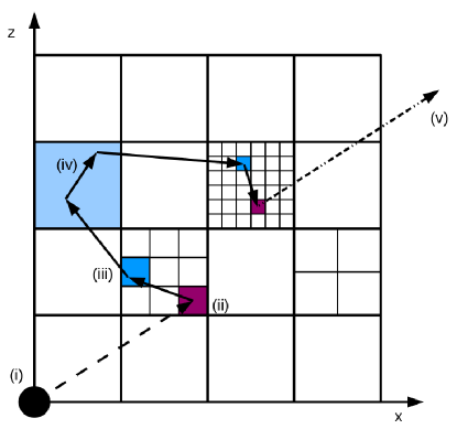
Figure 1.— 2D illustration of the three dimensional grid and the trajectories of the photon packets. The grid is divided into cubes, which can be further divided into sub-cubes. The source emits photons at (i), which interact or not with the dust. By interaction photon packets are either absorbed (ii) or scattered (iii). Multiple interactions may occur in one cell (iv). After absorption the packet will be re-emitted by the dust at a different frequency. Frequency changes are illustrated by different line styles. Finally, (v) the packet escapes the model space.

In our MC procedure the bolometric luminosity $L=\nolinebreak\int_{0}^{\infty}L_{\nu}d\nu$ of the central engine is divided into $N=m~{}n_{\rm{zyk}}$ monochromatic photon packets of equal energy $\xi=L/N$, where $m$ is the total number of frequency bins of the heating source and $n_{\rm{zyk}}$ counts the number of photon packets per bin. The width of the frequency bin with index j between the frequencies $\nu_{j}$ and $\nu_{j+1}$, $\Delta\nu=|\nu_{j+1}-\nu_{j}|$, is derived from the spectral shape of the radiation source and the energy of a photon packet

$$\xi=\int_{\displaystyle\nu_{j}}^{\displaystyle\nu_{j+1}}L_{\nu}d\nu~{}.$$ (1)

The primary heating source emits photons for example in the optical and UV while the dust emission occurs at IR and sub-millimeter wavelength. Two frequency grids are considered: The first one is set up by Eq. (1) and accounts for the emission of the primary heating source. The second frequency grid is an extended version of the first one and includes additional bins in the IR and sub-millimeter to scope with the dust emission. The interaction probability between photons and dust particles in the radiative transfer problem is computed by the absorption $\kappa^{abs}_{\nu}$ and scattering $\kappa^{sca}_{\nu}$ cross-sections. The code includes different grain materials and size distributions.

The model space is set up as cubes in an orthogonal Cartesian grid. Each cube is divided into an arbitrary number of sub-cubes of volume $V_{i}$ and constant density $\rho_{i}$ (Fig. 1), where the index refers to sub-cube $i$. The subdivision of cubes allows a finer sampling whenever required: For example close to the dust evaporation zone, in regions of high optical depth or where the spatial gradient of the radiation field is large. One possible trajectory of a photon is illustrated in Fig. 1. Photons are emitted by the source at frequency $\nu_{j_{\star}}$, where $j_{\star}$ is the index of the frequency grid of the source. The flight path of the photon through out the model space is computed.

The direction of the photon is chosen from a uniform distribution of random numbers $\zeta_{1},\zeta_{2}$ from the half open interval $[0,1)$, so that $\phi=2\pi\zeta_{1}$ and $\cos{\theta}=1-2\zeta_{2}$. The distance from the entry point of a photon into a cell $i$ to its exit point along the travel direction is $\ell_{i}$. In the MC method the interaction of photons with the dust in a sub-cube can be determined with an uniform distributed random number $\zeta$ (Witt 1977; Lucy 1999) and the optical depth

$$\tau_{i}(\nu)=(\kappa^{abs}_{\nu}+\kappa^{sca}_{\nu})\ \rho_{i}\ \ell_{i}~{}.$$ (2)

Photons leave the cell if $\tau_{i}(\nu)\leq-\log{\zeta}$ and otherwise they interact with the dust. If a packet passes through a cell without interacting, it enters a neighboring cell according to its direction of travel. At the border of the model space it eventually escapes. When a photon packet enters a cell a new random number is chosen to determine the interaction probability of photons with the dust . The photon packet interacts with the dust after it has traveled a distance

$$\ell_{i}^{\prime}=\frac{-\log{\zeta}}{\rho_{i}(\kappa^{abs}_{\nu}+\kappa^{sca}_{\nu})}~{}.$$ (3)

The travel distance $\ell_{i}^{\prime}$ defines the point in the cell where interaction takes place and photons are either scattered (Fig. 1.ii) or absorbed (Fig. 1.iii). Depending on its optical depth multiple scattering or absorption events may occur in a cell (Fig. 1.iv). In case of an interaction event the probability of scattering is given by the albedo $A_{\nu}=\kappa^{sca}_{\nu}\ /\ (\kappa^{sca}_{\nu}+\kappa^{abs}_{\nu})$ and therefore the chance of absorption is $1-A_{\nu}$.

When a photon is scattered on a dust grain the packet keeps its frequency, but changes its travel direction according to the phase function of the particle. We use the Henyey & Greenstein (1941) phase function to approximate the anisotropic scattering (see Sect. 4). In the isotropic case the asymmetry factor $g_{\nu}$ equals 0. The index of the cell, the frequency of the scattered photon and the incoming direction is stored. This allows computing of the source function of the cell $i$, which will be used in a ray–tracer developed to compute the observed image at any frequency (Sect. 4).

When a photon is absorbed a new one with different frequency and direction is emitted from that position. The frequency of the emitted photon packet is given by the temperature of the absorbing material. The emitted photon has the same energy as the absorbed one. All photon packets contain the same amount of energy $\xi$, therefore the total number of absorbed photon packets per particle and cell is used to calculate the temperature of each material. After $k$ absorptions of photon packets by dust the cell $i$ has a temperature $T_{i,k}$ calculated from:

$$\int{\kappa^{abs}_{\nu}B_{\nu}(T_{i,k})\ d\nu}\ =\ \frac{k\xi}{4\pi\rho_{i}V_{i}}~{},$$ (4)

where $B_{\nu}(T_{i,k})$ is the Planck function.

Dust emits a photon packet at the shortest frequency $\nu^{\prime}$ calculated with:

$$\int_{0}^{\nu^{\prime}}{\kappa^{abs}_{\nu}\ B_{\nu}(T_{i,k})\ d\nu}\ \geq\ \zeta\int_{0}^{\infty}{\kappa^{abs}_{\nu}\ B_{\nu}(T_{i,k})\ d\nu}~{}.$$ (5)

In the MC method one follows all $N$ photon packets through the dust cloud until they reach the outer boundary of the model and escape. For each cell the absorption events are counted. When all packets escaped the model space, the number of absorptions in a cell is used (Eq. (4)) to calculate its dust temperature. An iterative MC method is started with an initial guess of the dust temperatures. This allows computing of the frequencies of packets emitted by the dust (Eq. (5)). After all packets escape the model space another $N$ photons are emitted by the source and their flight paths through the model are computed. However, this time using the dust temperatures of the previous run. This procedure continues until the dust temperatures converges, which usually takes about 3–5 iterations.

2.1. Non equilibrium radiative transfer (PAH)

The enthalpy state of very small grains such as polycyclic aromatic hydrocarbons (Tielens 2008) fluctuates strongly when they are hit by photons. In order to solve the radiative transfer problem including PAH with MC we treat their emission as a stochastic process. A temperature distribution function $P(T)$ of the PAH is computed using the iterative scheme by Siebenmorgen et al. (1992). PAH are implemented into the MC code in two steps: first, we compute the PAH absorption of photon packages and store position and frequency of these events. Then, after calculating the equilibrium temperature of the large grains (Sect. 2), the PAH emission is computed. Each cell with PAH absorption becomes a source and emits the same number of photon packages as previously absorbed by the PAH. These photons are traced through the model as described in Sect. 2. The frequency of the emitted package is calculated according to:

$$\int_{0}^{\nu^{\prime}}\epsilon_{n}(\nu)d\nu\geq\xi\int\epsilon_{n}(\nu)d\nu\$$ (6)

with random number $\xi$ and PAH emissivity

$$\epsilon_{n}(\nu)=K^{\rm{PAH}}_{\nu}\int B_{\nu}(T)P_{n}(T)dT\ ,$$ (7)

where $K^{\rm{PAH}}_{\nu}$ is the PAH cross-section per unit mass of dust and $P_{n}(T)$ is the temperature distribution function as described in Siebenmorgen & Krügel (2010).

Similar to the evaporation of large grains it is important to compute the location where PAH are able to survive the radiation environment. We treat the photo–dissociation of PAH as discussed in Siebenmorgen & Krügel (2010). They find that PAH dissociate when, within a cooling time, the total absorbed energy $E_{\rm{PAH}}$ is larger than a critical energy $E_{\rm{crit}}:$

$$E_{\rm{PAH}}\geq E_{\rm{crit}}=\frac{N_{\rm C}}{2}\/\ {\rm{(eV)}},$$ (8)

where $N_{\rm{C}}$ is the number of carbon atoms per PAH molecule. In cells where the molecules dissociate the absorbed photon packages are treated as if they are emitted from the star. Further details on our and other numerical implementations of PAH in the MC code, a verification against benchmark models and an application to the PAH emission from proto–planetary disks is given in an accompanying paper (Siebenmorgen & Heymann 2012).

3. Optimized Monte Carlo radiative transfer

In this section we describe various optimization techniques which are introduced into our MC scheme to increase the accuracy and decrease computing times.

3.1. Small optical depth

The MC approach solves the radiative transfer problem in a probabilistic way. Dust temperatures become uncertain and have large errors whenever the interaction probability is low. This is the case in cells of low optical depth where many photons fly–by without being absorbed or scattered by the dust. The statistical noise in such cells can be reduced significantly applying a procedure developed by Lucy (1999). Contrary to the method described in Sect. 2, in which only absorption events contribute to the temperature calculation of the cell, the Lucy method considers the absorbed energy of every photon packet traveling through the cell. This technique increases the temperature accuracy of the MC treatment in low optical depth regions. It has no advantage when the optical depth $\tau_{i}\geq 1$ as interactions between photons and dust are likely.

We follow Sect.3.4 of Lucy (1999) and implement a similar optimization technique. It is applied whenever the maximal optical depth of a cell $i$ is smaller than $10^{-2}$. The performance of the MC scheme depends critically on this value. It is chosen so that the performance of the code is high while still accounting for reasonable accuracy. For smaller values the optimization is only applied for extreme optical thin cells whereas for higher values the expensive accuracy enhancement is applied to cells which can be accurately computed without the Lucy scheme. With our choice the energy absorbed by the dust $E^{\rm{abs}}_{i}$ is a small fraction of the energy of a photon packet. The energy is computed by

$$E^{\rm{abs}}_{\rm i}=(1-e^{-\tau_{\rm i}})\,\xi$$ (9)

where $\tau_{\rm i}$ is the optical depth from the entry to the exit point of the photon of cell $i$. Thereby the frequency of the photon packet remains unchanged.

3.2. High optical depth

The MC solution of the radiative transfer equation becomes slow for very optical thick regions, where the number of photon interactions with the dust increases exponentially. To avoid photons becoming trapped in cells with very high optical depth we apply a modified random walk procedure. It is based on a diffusion approximation by Fleck & Canfield (1984). The method is tested by Min et al. (2009) and numerical enhancements are given by Robitaille (2010).

3.3. Iteration–free Monte Carlo

An iteration free MC scheme is developed by Bjorkman & Wood (2001) (B&W); see Baes et al. (2005); Krügel (2008) for helpful comments. In the B&W method the dust temperature in a cell is adjusted with respect to the previous absorption event. Contrary to Eq. (5), dust re-emission occurs at the shortest frequency $\nu^{\prime}$ for which

$$\int_{0}^{\nu^{\prime}}{\kappa^{abs}_{\nu}\frac{dB_{\nu}(T_{i,k})}{dT}d\nu}\ \geq\ \zeta\int_{0}^{\infty}{\kappa^{abs}_{\nu}\frac{dB_{\nu}(T_{i,k})}{dT}\ d\nu}$$ (10)

is valid. Both methods described in Eq. (5) and Eq. (10) are implemented in the MC code and can be used upon preference.

3.4. Parallelization on graphics processing units

The MC method of solving the radiative transfer problem is particularly suited for parallelization because all photon packets are independent of each other (Jonsson 2006; Heymann 2010; Siebenmorgen et al. 2011). Vectorization of the code allows a number of photon packets to be emitted simultaneously. The number of packets launched at a time depends on the number of threads available on the computer. The trajectories of the photons can then be calculated in parallel.

In parallel environments an additional requirement is placed on the random number generator; each thread must have an independent sequence of random numbers. We solve this problem by applying a parallel version of the Mersenne Twister algorithm as given by Matsumoto & Nishimura (2000).

Parallelization is most efficient when all processing units finish their task at about the same time. Then vectorization speeds up the code roughly equal to the number of threads available. Unfortunately this is not always the case. The number of interactions of photons increases exponentially with the optical depth $\tau_{\rm{V}}$ and photon packets may get trapped in cells with say $\tau_{\rm{V}}\geq 1000$. The workload of these cells is much higher than for cells at much lower optical depth. This results in a rather unbalanced workload over all threads so that the advantage of vectorization may disappear. In our application idle threads are avoided as much as possible. Every time a thread finishes the trajectory of the photon packet within the model space a counter is increased. If the counter reaches $80\%$ of the total number of parallel working threads and if the number of interactions of the photon packet within a cell is larger than 100 the thread pauses. In this case the position and frequency of the photon packet is stored. Close to the end of the simulation when all photons with average processing speed have escaped the model space, the stored photons are resumed. This procedure allows a balanced workload among all threads. In addition the modified random walk procedure of Robitaille (2010) is implemented (Sect. 3.2.)

This code utilizes two different parallelization methods. It can be used on shared memory machines using the openMP library to run as many parallel rays as there are processor cores available and on vectorized hardware (GPU) highly optimized for parallelization. The complete MC radiative transfer solution is ported to GPU using the Compute Unified Device Architecture (CUDA) developed by NVIDIA (CUDA 2011). This speeds up the entire MC solution in comparison to the method by Jonsson & Primack (2010), which provides only a GPU acceleration when computing the temperature of a grain.

3.5. Numerical recipes

For vectorized MC radiative transfer codes it is recommended to follow some general recipes. In vectorized systems the increased number of processing units decreases the computing time for numerical operations whereas the time needed for read–and–write operations remains unaltered. This implies a paradigm shift in the programming strategy. In single processing codes the performance is often improved by reading pre–calculated values from memory. Instead in a vectorized code at some point it is faster to calculate such values case by case. For example in our code, and as long as the dust frequency grid has less than $300$ bins, it is faster to solve Eq. (5) on the fly than reading pre–computed values from memory.

The performance of parallel codes is increased considerably when designing a particular array structure for the particular hardware in use. A read operation from memory is most efficient when it accesses the entire array. For the GPUs used in this paper the memory bandwidth is 512 bit and we use a 32 bit machine. Therefore in our code the most efficient way to read from memory is by a modulus of $16\times 32$ bit values. The design of a particular array structure is import for problems where the memory access is not predictable, which is unfortunately the case in Monte Carlo schemes.

In order to improve the performance it is very efficient to code with as less interference between workers and threads as possible. The code should avoid situations where thread A waits until thread B has finished and then thread B waits until thread A has finished. Unfortunately in MC simulations the dependency between workers and threads is often less obvious than in the previous example.

Another challenge with memory interactions is to use local copies of arrays for each thread as often as possible. This decreases the interaction between different threads and usually leads to large performance improvements, of course at the expense of some additional memory needs. When dealing with memory interactions between threads it is helpful to study the special hardware capabilities. In our case we gain a factor 2 in the computing time by using atomic integer operations rather than floating point operations.

It is of advantage to optimize all read–and–write operations to the fastest available source. This can be done by caching small amounts of data from the disk to the global memory, than to the GPU memory and finally to the GPU shared memory. For example in our code we store the wavelength dependent cross–sections in the GPU shared memory. This is about 10 times faster than reading them from the global memory.

For MC simulations the random number generator (RNG) is important and special care must be taken on parallel systems. A detailed study of this topic is beyond the scope of this paper. We tested different RNG available and find that the performance and accuracy as well as thread dependence differs significantly between various RNG implementations. It is therefor important to choose and test a RNG which fits the particular problem best.

3.6. Parallelization and optimization algorithms

Table 1Run time requirements of different MC methods.

Method	Threads	Time
		(min.)
Lucy	$1$	180
B&W	$1$	60
Lucy	$8$	45
B&W	$8$	20
GPU	$256$	3
GPU+Lucy	$256$	4
GPU+B&W	$256$	2
GPU+B&W+Lucy	$256$	2

The run time requirements of the different MC methods are compared. We consider a star at temperature of 2500 K with solar luminosity which heats a spherical and constant density dust envelope with an inner radius of 0.7 AU and an outer radius of 700 AU. The optical depth measured from the star to the outer boundary is $\tau_{\rm{V}}=10$. Parameters of the dust are specified as in Sect. 5.1. In the models $10^{7}$ photon packets are emitted from the star and $10^{6}$ grid cells are used.

We apply the Lucy (Sect.3.1), B&W (Sect.3.3.) method in a scalar (single thread), a CPU version with 8 threads, a GPU version with 256 threads and in addition the iterative MC scheme of Sect. 2 on a GPU machine. Initializing times of the various MC methods are identical.

As described in Sect.3.1 for the same number of emitted photon packets the Lucy method provides a better temperature estimate than the other methods. In the Lucy method the fraction of a photon packet is considered. This can only be realized by considering floating point operations which are more computer expensive than integer operations. In our test case the scalar version of the Lucy method is run with three iterations and requires a total run time of 3 hours (Tab. 1).

For single thread applications the iteration–free MC scheme by B&W (Sect. 3.3) has the advantages that it speeds up the process by a factor which equals the number of iterations required for convergence in the other MC treatments. However, in the B&W method memory interaction between different cells are unavoidable and they slow down the parallelization capabilities of this method. The memory interaction between cells rises with the number of threads and therefore the amount of necessary atomic memory operations increases with parallelization. To minimize the number of atomic memory operations we solve the problem in an iterative MC scheme using Eq. (4). This allows parallelization with a huge number of threads. At low budget this can be realized using GPU technology and these MC methods are labeled as such in column 1 of Table 1. The GPU method may be further optimized in combination with the Lucy (GPU+Lucy) or the B&W method (GPU+B&W). On our conventional computer we use a GPU with 256 threads (8 multiprocessor each with 32 cores) clocked at 1.5 GHz. When compared to a single thread CPU application clocked at 3 GHz a speed up factor due to vectorization of 60 is realized. This is below a theoretical expected speed up factor of 128 because of additional overheads produced by input/output routines and memory transfers in the GPU machine.

Total run times of the various methods with different numbers of threads are given in Table 1. The vectorized Lucy method scales slightly better with the number of available threads than the other algorithms because fewer atomic memory operations are required. The speed increase by vectorization as compared to scalar MC treatments is proportional to the number of available threads. The GPU method with B&W optimization is a factor 90 faster than the original Lucy method.

4. Ray–tracer to compute SEDs and images

Photons which eventually escape the MC model space in a particular solid angle can be counted and converted into a flux density. In principle this method allows computing images of the object. Unfortunately to obtain a moderate signal–to–noise ratio the number of photon counts per solid angle must be high which is difficult to reach within reasonable computing times. Here we present a ray–tracing method which allows computing of noise free images, SEDs and visibilities at high spatial resolution. The ray–tracer uses the temperature and scattering events of the cells calculated with the MC code (Sect. 2). The uncertainty in the derived images is therefore based on the precision of the MC computation.

In the algorithm rays are traced through the model space from an observer plane of arbitrary orientation. The ray tracer together with the MC method allows us to calculate the flux received on each pixel of an image in the plane of the observer. The observed image is located at distance $D$ from the object which is at the center of the cube. The orientation of the image plane is defined by its surface normal $\vec{~{}e_{z}}^{\prime}$. The axis of the image plane $\vec{~{}e_{x}}^{\prime},\vec{~{}e_{y}}^{\prime}$ is perpendicular to $\vec{~{}e_{z}}^{\prime}$. The coordinates $(x,y,z)$ of the 3D model space are transformed by a parallel projection into the coordinates $(x^{\prime},y^{\prime})$ of the 2D image in the observers plane. The image consists of $n_{x}\times n_{y}$ pixels, with a pixel size chosen so that the complete model fits in the projection. The center of the image $\vec{i}_{0}$ is located at position $[x_{0},y_{0},z_{0}]$ and has image coordinates $[x^{\prime}_{0},y^{\prime}_{0}]$. The projected coordinates $[x^{\prime},y^{\prime}]$ of the image are transformed into MC cube coordinates by

$$\vec{r}(x^{\prime},y^{\prime})=\vec{i}_{0}+(x^{\prime}-x^{\prime}_{0})\vec{~{}e_{x}}^{\prime}+(y^{\prime}-y^{\prime}_{0})\vec{~{}e_{y}}^{\prime}~{},$$ (11)

where $\vec{r}=[x,y,z]$. The ray–tracer follows the line of sight from each detector pixel in direction $\vec{~{}e_{z}}^{\prime}$ through the MC model. Adding the contribution of emission and scattering from each cell $i$ along the line of sight results in the observed intensity. The contribution of cell $i$ to the total intensity is

$$I_{\nu,i}=(I^{e}_{\nu,i}+I^{s}_{\nu,i})~{}e^{-\tau_{\nu,i}}~{},$$ (12)

where $I^{e}_{\nu,i}$ refers to the intensity of the dust emission and $I^{s}_{\nu,i}$ to scattering; $\tau_{\nu,i}$ is the optical depth at frequency $\nu$ of cell $i$. For convenience we drop the index $i$ in the following. The optical depth is

$$\tau_{\nu}=\mathrm{K}^{abs}_{\nu}\int_{0}^{\ell}\rho\,(\vec{r})\,ds~{},$$ (13)

where $K^{abs}_{\nu}$ is the absorption cross section per unit dust mass and $\ell$ is the path lengths. We call the optical depth measured along the ray from the border of the cell to the observer $\tau_{\nu}$, and the one measured face–to–face from one side of the cell to the other $\tau^{\rm cell}_{\nu}$. The emission is

$$I_{\nu}^{e}=\big{[}1-\rm{exp}(-\tau^{\rm cell}_{\nu})\big{]}~{}\mathrm{B_{\nu}}(T)~{}.$$ (14)

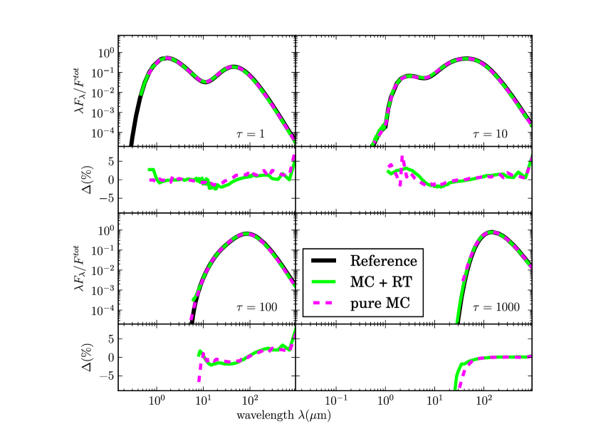
Figure 2.— Comparison of SEDs of dust spheres at optical depths between $\tau_{\rm{V}}=1$ and 1000 computed with MC and ray–tracer (green) or photon counting (dashed), benchmark results in black (Ivezic et al. (1997)). Lower panels give the difference between benchmark and the procedures of this work.

For scattering we implement either a g–factor approximation following the notation of Krügel (2008) or consider non–isotropic scattering applying the Henyey–Greenstein phase function $P_{\rm HG}$ (Henyey & Greenstein 1941) defined as:

$$P_{\rm HG}(\beta)=\frac{1}{4\pi}\frac{(1-g^{2})}{~{}\big{[}1+g^{2}-2g~{}\rm{cos}(\beta)\big{]}^{3/2}},$$ (15)

where g is the anisotropy parameter. If $g=0$ the scattering is isotropic. The scattered light intensity is given by

$$I^{s}_{\nu}=\sum_{\beta}P_{\rm HG}(\beta)\frac{N(\beta,\nu)^{sca}~{}\epsilon}{\Delta\nu}~{},$$ (16)

where $\Delta\nu$ is the width of the frequency bin, $N(\beta,\nu)^{sca}$ is the total number of scattering events with frequency $\nu$ and angle $\beta$ between the observer and the original scattering direction. This method to calculate the scattered intensity is similar to the peel–off technique proposed by Yusef-Zadeh et al. (1984). The difference lies in the time of the calculation of the scattering intensity. The peel–off technique calculates the intensity during the MC run. Whenever a scattering event occurs the scattered intensity of the event is added to the observed images. Therefore in the peel–off technique the location of the observer has to be known before the MC run. This information is not required in our MC scheme which stores only the scattering events. Then, in post–processing using the ray–tracer, the contribution of the scattered light flux can be computed for arbitrary observer orientations. The flux density is calculated summing up the contribution of each cell given by

$$F_{\nu,\mathrm{i}}=\frac{A_{\rm pix}}{D^{2}}\big{[}I_{\nu}^{e}+I^{s}(\theta)\big{]}\ \rm{exp}(-\tau_{\nu})~{},$$ (17)

where $\tau_{\nu}$ is the optical depth from the border of the cell to the observer and $A_{\rm pix}$ is the area of the detector pixel. The ray–tracer calculates emission and scattering images at high signal–to–noise. It cannot remove the noise which is introduced by the MC simulation where the temperature distribution and scattering events are calculated with a stochastic sampling. However, for a known distribution of the temperature and scattering events the ray–tracer provides noise free images.

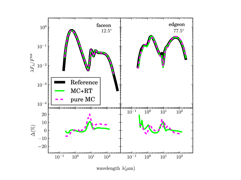
Figure 3.— Comparison of SEDs of a dust disk at optical depths along the midplane of $\tau_{\rm{V}}=100$, face–on view ($12.5^{\circ}$) is shown left and edge–on view ($77.5^{\circ}$) right. SEDs are computed with MC and ray–tracer (green) or photon counting (dashed). The mean SED of the benchmark results by Pascucci et al. (2004) is in black. Lower panels give the difference between the mean SED of the benchmark and the procedures of this work.

5. Benchmark

The vectorized MC method is tested against the 1d ray tracing code by Krügel (2008). Further verifications of the MC and comparison with benchmark tests are described below

5.1. Spherical symmetry (1D)

Benchmark models in 1D are provided by Ivezic et al. (1997). They consider a spherical dust envelope which is centrally heated by a 2500 K star with luminosity of $1L_{\sun}$. For this test the dust absorption and scattering coefficient for wavelength below $\lambda_{0}=1\mu$m are $q_{\rm{abs}}=q_{\rm{sca}}=1$ and are $q_{\rm{sca}}=\lambda_{0}/\lambda$ and $q_{\rm{abs}}=(\lambda_{0}/\lambda)^{-4}$ at longer wavelengths. Models are computed at optical depths of $\tau_{\rm{V}}=1$, 10, 100 and 1000 with inner radius $r_{\rm{in}}=3.14$, 3.15, 3.20 and 3.52 AU, respectively. The dust density is constant and the outer radius is $r_{\rm{out}}=1000\times r_{\rm{in}}$. The models are run on a grid with $10^{6}$ cells and $2\times 10^{8}$ photon packets per iteration are launched from the star. The number of MC iterations are 3, 4 and 5 for $\tau_{\rm{V}}\leq 10$, 100 and 1000, respectively.

MC computed temperatures are compared to the one calculated by DUSTY (Ivezic & Elitzur 1997) and Krügel (2008); they agree within $\mathbin{\lower 3.0pt\hbox{$\hbox to0.0pt{\raise 5.0pt\hbox{$\char 60\relax$}\hss}\mathchar 29208\relax$}}1$ %. The SEDs are shown in Fig. 2 in which each quadrant represents models at different optical depths. In the quadrants the SED are shown in the top and the flux difference between MC and benchmark in the bottom panel. The SED of the MC models are either computed by photon counting or using the ray–tracer (Sect. 4). The difference of the SED computed by MC and DUSTY is typically better than a few %. It becomes larger at faint fluxes where the ray tracing is more accurate than the packet counting procedure because of photon noise. For the $\tau_{\rm{V}}=1000$ model the counting method is starved at fluxes below 0.2% from the peak flux. We encountered numerical inconsistencies in the DUSTY code at flux levels $\mathbin{\lower 3.0pt\hbox{$\hbox to0.0pt{\raise 5.0pt\hbox{$\char 60\relax$}\hss}\mathchar 29208\relax$}}10^{-8}$ from the peak when compared against the radiative transfer code by Krügel (2008).

The differences between the reference codes and our MC program is mainly caused by Poisson noise. The photon noise is large at flux levels which are low compared to the peak flux. The wavelength range where the frequency grid of the source and that of the dust overlap is an additional source of systematic error. The source grid is build so that the energy of the photon packets of each frequency bin are identical. This results in a larger bin size at the Rayleigh–Jeans tail of the star where, on the other hand, the dust grid has a fine sampling because of the silicate and PAH features. To reduce this sampling problem it is necessary to increase the number of frequency bins of the star. Unfortunately, the total number of photons emitted from the star must be increased to achieve a certain signal–to–noise for each bin. The number of photons emitted from the star in each frequency bin must be large enough to reduce the Poisson noise to acceptable levels. We use $1000$ frequency bins for the star and emit in each bin $10^{5}$ photons. This choice is based on a run time optimization for the achieved accuracy. The third source of systematic differences between the reference codes and our MC scheme is the spatial grid. While the MC code uses a Cartesian grid in three dimensions with one level of refinement the reference codes and in particular that of Krügel (2008), uses an extremely optimized grid to account for the spherical symmetry. This systematic effect could be reduced by an increase of the number of MC grid cells. Current hardware limits the number of grid cells because of memory and speed constraints.

5.2. Disk geometry (2D)

Table 2Parameters of 2D benchmark by Pascucci et al. (2004)

Symbol	Parameter	Value
$\rm{M}_{\star}$	Stellar Mass	$1\ \rm{M}_{\sun}$
$\rm{R}_{\star}$	Stellar Radius	$1\ \rm{R}_{\sun}$
$\rm{T}_{\star}$	Stellar effective temperature	$5800\rm{K}$
$r_{\rm{in}}$	Inner disk radius	$1\ \rm{AU}$
$r_{\rm{out}}$	Outer disk radius	$1000\ \rm{AU}$
$r_{d}$	Half of outer radius	$500\ \rm{AU}$
$z_{d}$	Disk height	$125\ \rm{AU}$
$\rm{a}$	Grain radius	$0.12\ \mu\rm{m}$
$\rm{\rho}_{0}$	Density for $\tau_{\rm{V}}=1$	$8.45\,10^{-22}\rm{g}\rm{cm}^{-3}$
$\rm{\tau}_{\rm{v}}$	Optical depth at 550 nm	$1,10,100$

Different methods to compute the RT in a 2D dust configuration are compared by Pascucci et al. (2004). They consider a star which heats a dust disk. The inner region $r<r_{\rm{in}}$ is dust free and the dust density distribution is similar to those described by Chiang & Goldreich (1997, 1999):

$$\rho(r,z)=\rho_{0}~{}(\frac{r_{d}}{r})~{}e^{-(0.25\pi(z/h)^{2})}$$ (18)

with

$$h=z_{d}~{}(\frac{r}{r_{d}})^{1.125}~{},$$ (19)

where $r$ is the distance from the central star in the midplane of the disc and $z$ is the height above the midplane. The parameter $\rho_{0}$ is chosen such that the optical depth at 550 nm along the midplane is 1, 10 and 100, which leads to densities $\rho_{0}=8.45\,10^{-22},8.45\,10^{-21}$ and $8.45\,10^{-20}$ g cm^-3. Additional parameters are specified in Table 2. The absorption and scattering cross sections are that of a 0.12$\mu$m silicate grain (optical data are taken from Draine & Lee (1984)).

The SEDs calculated by the various algorithms and treatments used by Pascucci et al. (2004) agree to better than 20%. The RT in the disk is solved by our GPU code and the derived SED are compared to an averaged SED of the results given by Pascucci et al. (2004)

In the MC program we use $~{}3\times 10^{6}$ cells and run models with $~{}2\times 10^{8}$ photon packets per iteration.

For the optical depth along the midplane of the disk with $\tau_{\rm{V}}\leq 10$ we use 3 iterations and found in the SED an overall agreement to the benchmark results to within a few %. In the $\tau_{\rm{V}}=100$ case 4 iterations are used and the SED and differences to a mean SED over those computed in the reference models is shown in Fig. 3. Two different inclinations $12.5^{\circ}$ (face–on), $77.5^{\circ}$ (edge–on) are displayed. The residual between SED computed by us and the mean SED of the benchmarks is typically a few % and larger deviation are found at fluxes below 1% of the peak flux. This is visible at the border of the wavelength grid and in the 10$\mu$m silicate absorption band where variations from one SED to another in the reference codes are also larger.

The differences in the two dimensional benchmark and our code are twofold. There is the Poisson noise which is present in our as well as in the reference. Note that the reference SED in Pascucci et al. (2004) is computed as an average of various SEDs computed by different codes. The second source of systematic error is the grid. We use a three dimensional Cartesian grid with one level of refinement. The reference codes calculate the benchmark in a two dimensional grid optimized to account for the disc symmetry. It is possible to improve our solution by increasing the number of grid cells as well as the number of photon packages. However, the current hardware gives an upper limit to run time and memory requirements.

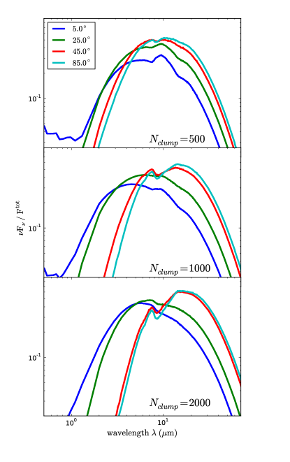
Figure 4.— Spectral energy distribution of clumpy AGN torus models at viewing angles between $5^{\circ}$ and $85^{\circ}$ and number of clouds of $N_{\rm{clump}}=500$, 1000 and 2000.

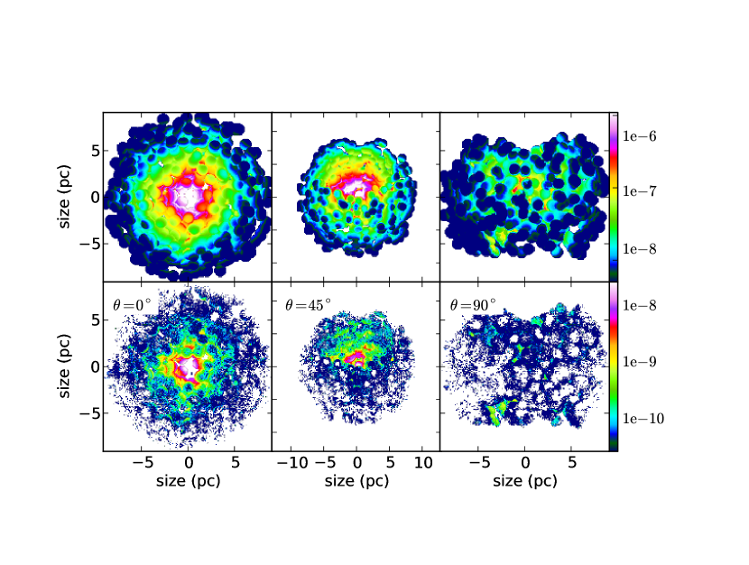
Figure 5.— Images at 10$\mu$m (top) and 0.55$\mu$m (bottom) of the clumpy AGN torus with $N_{\rm{clump}}=1000$ and viewing angles (from left to right) of $0^{\circ}$, $45^{\circ}$ and $90^{\circ}$. . Color bar gives flux in (Jy/arcsec²). The source with luminosity L=10⁴⁵ erg/s is at a distance of 15 Mpc

6. Clumpy AGN torus model

The unified scheme of AGN (Antonucci & Miller 1985; Padovani & Urry 1990) predict that the central engine is surrounded by dust so that the obscuration depends on the viewing angle. The detailed geometrical configuration of dust around the AGN is still a matter of debate (Stalevski et al. 2011). Observations are not able to resolve the inner part of the objects. Theoretical considerations favor a toroidal and clumpy geometry (Nenkova et al. 2002; Schartmann et al. 2005; Hönig et al. 2006; Nenkova et al. 2008; Schartmann et al. 2008, 2010). Observational hints of a clumpy structure in which optically thick dust clouds surround the accretion disc of the central black hole are provided by the 10$\mu m$ silicate band. This band is detected in absorption and emission. The strength of the feature is much weaker than predicted by homogeneous torus models (Pier & Krolik 1992; Granato & Danese 1994; Efstathiou & Rowan-Robinson 1995; van Bemmel & Dullemond 2003). A silicate emission feature is also seen in obscured AGN, where the broad emission lines are hidden (Sturm et al. 2006; Mason et al. 2009). Observations are explained by postulating a clumpy torus structure.

For the dust around AGN we consider fluffy agglomerates of silicate and carbon as sub–particles. We use a power law size distribution: $n(a)\propto a^{-3.5}$ with particle radii between $a_{-}\leq a\leq a_{+}$ and $a_{-}=160\rm{\AA}$ , $a_{+}=0.13\mu$m. The bulk density of both materials is 2.5 g/cm³. Dust abundances (ppm) are 31 [Si]/[H] and 200 [C]/[H], which agree with cosmic abundance constraints (Asplund et al. 2009). This gives a gas–to–dust mass ratio of 130. We take the relative volume fractions in composite grain to be 34% silicates, 16% carbon and 50% vacuum, which translates, with abundances as above, to a relative mass fraction of 68% silicates and 32% amorphous carbon. Absorption and scattering cross–sections and the scattering asymmetry factor is computed with Mie theory and the Bruggeman mixing rule. Optical constants for silicates are taken from Draine (2003) and for carbon we use the ACH2 mixture from Zubko et al. (1996). This gives a total mass extinction cross section in the optical (0.55$\mu$m) of $K^{ext}_{V}=35000$. The wavelength dependence of $K^{ext}$ is displayed in Kruegel & Siebenmorgen (1994).

The hard (UV/optical) AGN radiation emerges from the accretion disc around the massive black hole. Its spectral shape is suggested to follow a broken power law (Rowan-Robinson 1995):

$$\lambda F_{\lambda}\propto\left\{\begin{array}[]{ccl}\lambda^{1.2}&\text{for}&~{}-\infty<~{}\lambda~{}<0.01\mu{\rm m}\\ \ {\rm{const}}&\text{for}&~{}~{}0.01<~{}\lambda~{}<0.10\mu{\rm m}\\ \lambda^{-0.5}&\text{for}&~{}~{}0.1~{}~{}<~{}\lambda~{}<~{}~{}1.0\mu{\rm m}\\ \lambda^{-3}&\text{for}&~{}~{}1.0~{}~{}<~{}\lambda~{}<+\infty\\ \end{array}\right.$$ (20)

In the following we consider a clumpy AGN dust torus of total luminosity of $L_{45}=10^{45}$ erg/s. The inner radius of the torus $r_{\rm{in}}$ is set by dust evaporation, which is approximated by $r_{\rm{in}}=0.4~{}(L_{45})^{0.5}\,\rm{pc}$. A clump is represented as a sphere of constant density and radius of 0.5 pc. The optical depth through the center of the clump is $\tau_{\rm{V}}=30$. The clumps are randomly distributed within a half opening angle of $\theta=45^{\circ}$ between an inner radius of $r_{\rm{in}}=0.4$ pc and outer radius of $r_{\rm{out}}=6$ pc. For random numbers $\zeta_{1},\zeta_{2},\zeta_{3}$ the position of the center of the clouds is computed by

$$r = \zeta_{1}~{}(r_{\rm{out}}-r_{\rm{in}})$$

$$\phi = 2\pi~{}\zeta_{2}$$ (21)

$$\theta = \frac{\pi}{2}+(2~{}\zeta_{3}-1)\theta_{1}~{}.$$

If clumps overlap the density is constant and the same as for a single clump.

6.1. Influence on clumps on SED

The AGN torus model is used to study the influence of clumps on the SED. In the models the number of clouds is varied using $N_{\rm{clump}}=500,1000$ and $2000$. This gives a total optical depth along the midplane of the torus of $\tau_{\rm{V}}\sim 80$, 140 and 200. The SED is displayed in Fig. 4; at wavelengths $\mathbin{\lower 3.0pt\hbox{$\hbox to0.0pt{\raise 5.0pt\hbox{$\char 60\relax$}\hss}\mathchar 29208\relax$}}\,1\,\mu\rm{m}$, the flux is emitted by the central source and between 1$\mu$m and 50$\mu$m the SED is dominated by dust emission. The dust temperatures are between 100 and 1500 K. At short wavelengths of the SED the AGN is visible only in the face–on view and becomes faint at higher inclination angles. At longer wavelengths the flux is stronger in the edge–on view as compared to observations at smaller inclination angles. The optical depth of a single clump is high and already one or two of such intervening clouds define most of the spectral behavior of the torus. The SEDs at viewing angles between $45^{\circ}$ and $85^{\circ}$ are similar. At these angles a few clouds are always in the line of sight and dominate the spectrum (Fig. 4).

Depending on the viewing angle and the total optical depth and dust temperatures in the AGN, the 10 $\mu$m silicate band is observed either in emission or in absorption. In AGN viewed face–on (type I sources) there is a direct view on the inner region of the torus and a weak $10\mu$m silicate emission feature is observed (Siebenmorgen et al. 2005; Hao et al. 2005; Sturm et al. 2005). In edge–on sources (type II) the $10\mu$m silicate band is seen in absorption.

The silicate feature trace the amount of dust for a given viewing direction and constraints the distribution of the clumps in the torus (Nikutta et al. 2009). Homogeneous AGN torus models without a clumpy structure over–predict the strength of the silicate feature (Efstathiou & Rowan-Robinson 1995). In the clumpy torus models presented in Fig. 4 the $10\mu$m feature is in emission for face–on views as long as $N_{\rm{clump}}\mathbin{\lower 3.0pt\hbox{$\hbox to0.0pt{\raise 5.0pt\hbox{$\char 60\relax$}\hss}\mathchar 29208\relax$}}1000$. Individual clouds are optically thick at $10\mu$m so that a single cloud already obscures the warm and optical thin region required to observe the silicate band in emission. This is the case in the face–on view of the model with 2000 clumps where the emission and self–absorption of the silicate grains cancels out and the spectrum becomes featureless. For inclination angles $\theta\geq 45^{\circ}$ the silicate features is in absorption (Roche et al. 1991). The strength of the absorption feature depends on the optical depth and therefore increases with increasing number of clumps.

6.2. AGN images

The MC combined with the ray–tracer (Sect. 4) allows computing of images of the object at a given wavelength. In Fig. 5 we present a $10\mu$m and $0.55\mu$m image of the clumpy AGN torus using $N_{\rm{clump}}=1000$. The mid IR image is dominated by dust emission and the optical image by scattered light. The face–on image in the mid IR provides an unobscured view of the emission from hot dust in the inner torus close to the AGN. In this image, clouds near the center dominate the emission. Further out, clumps become cooler and the contribution to the emission decreases. In the tilted view, at $45^{\circ}$, intervening clumps obscure part of the emission from the central region and the contribution of cooler dust becomes more important than in the face–on view. In the edge–on view most of the central region is no longer visible and the emission is dominated by clouds located close to the border of the torus. However, close to the edge–on view and because of the clumpy nature of the medium there are still a few lines of sight penetrating to the inner torus. This is not the case in AGN models using a homogeneous dust distribution. For all viewing angles and clump configurations the scattered light images appear similar to the emission images (Fig. 5). However, the flux in the optical is two orders of magnitude fainter than at 10$\mu$m. The scattering light image in the edge–on view becomes fuzzy. The assumption of isotropic scattering likely over predicts the scattered light in the face–on direction. However, the clumpy structure visible in the optical image is preserved.

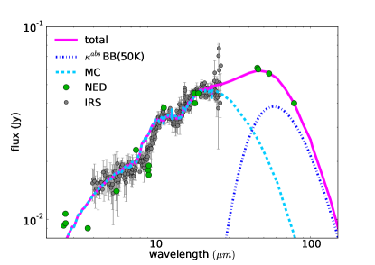
Figure 6.— IR emission of the quasar 3C249.1. Photometric data by NED and Spitzer spectrum by Siebenmorgen et al. (2005). The total flux (full line) is given as sum of the clumpy AGN torus model (dashed) and a cirrus component (dashed dotted).

6.3. Quasar 3C 249.1

The clumpy AGN dust torus model is applied to fit the SED of the quasar 3C249.1. The luminosity of the object is $7\times 10^{45}$ erg/s at redshift of $z=0.311$ which translates, using standard cosmological parameters, to a luminosity distance of 1600 Mpc. The torus inner edge is set by the sublimation temperature and leads to an inner radius of $r_{\rm{in}}=1$ pc. In the inner region of the model at $r\leq 25\times r_{\rm{in}}$ the half opening angle of the torus is $\theta_{1}=25^{\circ}$ and in the outer region up to $r_{\rm{out}}=50\times r_{\rm{in}}$ it is $55^{\circ}$. The torus includes 5500 clouds. The number of clumps per volume element decreases in the inner part and increases in the outer part of the torus; other parameters remain the same.

In order to fit data at $\lambda>40\mu$m we increased the outer radius of the torus $r_{\rm{out}}$ and considered a two phase medium in which the density in between the clumps is varied. However, the far IR emission of the quasar cannot be explained by the AGN torus. The far IR is dominated by emission of cold dust located furtherout in the host galaxy. For simplicity we approximate this cirrus component by a modified black body, $\kappa_{\nu}^{abs}B_{\nu}(T)$ at 50 K. The dust torus model fits the silicate emission feature as observed in the Spitzer spectrum and together with the cirrus component a good fit to the overall SED is achieved (Fig. 6).

7. Conclusions

A parallel 3D MC method is presented to solve the radiative transfer problem of dust obscured objects in arbitrary geometries. The code uses an adaptive three dimensional Cartesian grid. It utilizes the advantage of different optimization algorithms: in optical thin cells the Lucy algorithm and in cells at very high optical depths a modified random walk procedure by Fleck & Canfield (1984) is included. The temperature of the dust is computed in an iterative MC method or with the iteration–free Bjorkman & Wood (2001) algorithm.

The spectral energy distribution of the objects is derived by a photon counting procedure or a ray–tracing routine. Photons which eventually escape the MC model space are counted and converted into a flux density. This method computes the SED of an object very quickly when a large aperture of several degree is used. Unfortunately, for high spatial resolution the method is starved by the low count rate. The SED of an object observed with a pencil beam is computed by a ray tracer which uses the dust scattering and absorption events of the MC cells as input. The ray tracer allows computing of noise free images of the scattered and emitted radiation at any frequency.

MC schemes are known to be computing time expensive. Therefore we apply particular attention to solve this problem. We take advantage of the independence of the trajectories of each photon packet. This allows a highly vectorized design of the MC program which is not realized in previous work. With the vectorized code a speed improvement of about 100 is reached on a low budget computer when compared to a scalar, non–parallel version of the same program. This gain in the speed performance of the computations is reached by applying either a multi–core application using conventional central processing units (CPU) or the recent technological development of graphics power units (GPU). The parallelization capabilities of various MC radiative transfer algorithms are analyzed. By combining different MC algorithms we report a linear scaling of the computing time with the number of available threads (processor cores). The ray–tracer to compute SED and images is another computer time expensive procedure and is developed, similar to the MC code, in vectorized form.

The 3D MC is tested against the ray tracer solution of the radiative transfer problem in spherical symmetry by Krügel (2008). Further we verified our procedure against one and two dimensional benchmarks of the literature. The code reproduces the spectral energy and dust temperature distributions of the test cases at high accuracy. As a first astrophysical application we use the MC code to investigate the appearance of a dusty AGN at optical and IR wavelengths; a second application on proto–planetary disks is presented in an accompanying paper (Siebenmorgen & Heymann 2011)

The dust around the AGN is geometrically configured in a clumpy torus structure and is represented by fluffy composite grains of various sizes made of silicate and carbon. The influence of the number of clumps in the torus on the SED is studied. We find that the clumpy torus explains the observed “weak” silicate absorption and emission feature observed in AGN. Images of the AGN in the optical and the mid IR are presented by viewing the torus from different angles. The spectral energy distribution of the radio loud quasar 3C249.1 is fit by the torus model including a cirrus component for the far IR and submillimeter emission.

References

- Antonucci & Miller (1985) Antonucci, R. R. J. & Miller, J. S. 1985, ApJ, 297, 621
- Asplund et al. (2009) Asplund, M., Grevesse, N., Sauval, A. J., & Scott, P. 2009, ARA&A, 47, 481
- Baes (2008) Baes, M. 2008, MNRAS, 391, 617
- Baes et al. (2005) Baes, M., Stamatellos, D., Davies, J. I., et al. 2005, New Astronomy, 10, 523
- Baes et al. (2011) Baes, M., Verstappen, J., De Looze, I., et al. 2011, ApJS, 196, 22
- Bianchi (2008) Bianchi, S. 2008, A&A, 490, 461
- Bjorkman & Wood (2001) Bjorkman, J. E. & Wood, K. 2001, ApJ, 554, 615
- Chiang & Goldreich (1997) Chiang, E. I. & Goldreich, P. 1997, ApJ, 490, 368
- Chiang & Goldreich (1999) Chiang, E. I. & Goldreich, P. 1999, ApJ, 519, 279
- CUDA (2011) CUDA. 2011, NVIDIA C Programming Guide
- Draine (2003) Draine, B. T. 2003, ApJ, 598, 1017
- Draine & Lee (1984) Draine, B. T. & Lee, H. M. 1984, ApJ, 285, 89
- Efstathiou & Rowan-Robinson (1995) Efstathiou, A. & Rowan-Robinson, M. 1995, MNRAS, 273, 649
- Fleck & Canfield (1984) Fleck, J. J. & Canfield, E. 1984, Journal of Computational Physics, 54, 508
- Gordon et al. (2001) Gordon, K. D., Misselt, K. A., Witt, A. N., & Clayton, G. C. 2001, ApJ, 551, 269
- Granato & Danese (1994) Granato, G. L. & Danese, L. 1994, MNRAS, 268, 235
- Haas et al. (2008) Haas, M., Willner, S. P., Heymann, F., et al. 2008, ApJ, 688, 122
- Hao et al. (2005) Hao, L., Spoon, H. W. W., Sloan, G. C., et al. 2005, ApJ, 625, L75
- Henyey & Greenstein (1941) Henyey, L. G. & Greenstein, J. L. 1941, ApJ, 93, 70
- Heymann (2010) Heymann, F. 2010, PhD thesis, University of Bochum, ”http://www-brs.ub.ruhr-uni-bochum.de/netahtml/HSS/Diss /HeymannFrank/diss.pdf”
- Hönig et al. (2006) Hönig, S. F., Beckert, T., Ohnaka, K., & Weigelt, G. 2006, A&A, 452, 459
- Ivezic & Elitzur (1997) Ivezic, Z. & Elitzur, M. 1997, MNRAS, 287, 799
- Ivezic et al. (1997) Ivezic, Z., Groenewegen, M. A. T., Men’shchikov, A., & Szczerba, R. 1997, MNRAS, 291, 121
- Jonsson (2006) Jonsson, P. 2006, MNRAS, 372, 2
- Jonsson & Primack (2010) Jonsson, P. & Primack, J. R. 2010, arXiv, 15, 509
- Krolik & Begelman (1988) Krolik, J. H. & Begelman, M. C. 1988, ApJ, 329, 702
- Kruegel & Siebenmorgen (1994) Kruegel, E. & Siebenmorgen, R. 1994, A&A, 288, 929
- Krügel (2008) Krügel, E. 2008, An introduction to the physics of interstellar dust (Springer)
- Lucy (1999) Lucy, L. B. 1999, A&A, 344, 282
- Mason et al. (2009) Mason, R. E., Levenson, N. A., Shi, Y., et al. 2009, ApJ, 693, L136
- Matsumoto & Nishimura (2000) Matsumoto, M. & Nishimura, T. 2000, in Monte Carlo and Quasi-Monte Carlo Methods 1998 (Springer), 59–69
- Min et al. (2009) Min, M., Dullemond, C. P., Dominik, C., de Koter, A., & Hovenier, J. W. 2009, A&A, 497, 155
- Misselt et al. (2001) Misselt, K. A., Gordon, K. D., Clayton, G. C., & Wolff, M. J. 2001, ApJ, 551, 277
- Nenkova et al. (2002) Nenkova, M., Ivezić, Ž., & Elitzur, M. 2002, ApJ, 570, L9
- Nenkova et al. (2008) Nenkova, M., Sirocky, M. M., Ivezić, Ž., & Elitzur, M. 2008, ApJ, 685, 147
- Nikutta et al. (2009) Nikutta, R., Elitzur, M., & Lacy, M. 2009, ApJ, 707, 1550
- Padovani & Urry (1990) Padovani, P. & Urry, C. M. 1990, ApJ, 356, 75
- Pascucci et al. (2004) Pascucci, I., Wolf, S., Steinacker, J., et al. 2004, A&A, 417, 793
- Pier & Krolik (1992) Pier, E. A. & Krolik, J. H. 1992, ApJ, 399, L23
- Robitaille (2010) Robitaille, T. P. 2010, A&A, 520, A70+
- Roche et al. (1991) Roche, P. F., Aitken, D. K., Smith, C. H., & Ward, M. J. 1991, MNRAS, 248, 606
- Rowan-Robinson (1995) Rowan-Robinson, M. 1995, MNRAS, 272, 737
- Schartmann et al. (2010) Schartmann, M., Burkert, A., Krause, M., et al. 2010, MNRAS, 403, 1801
- Schartmann et al. (2005) Schartmann, M., Meisenheimer, K., Camenzind, M., Wolf, S., & Henning, T. 2005, A&A, 437, 861
- Schartmann et al. (2008) Schartmann, M., Meisenheimer, K., Camenzind, M., et al. 2008, A&A, 482, 67
- Siebenmorgen et al. (2005) Siebenmorgen, R., Haas, M., Krügel, E., & Schulz, B. 2005, A&A, 436, L5
- Siebenmorgen & Heymann (2011) Siebenmorgen, R. & Heymann, F. 2011, A&A
- Siebenmorgen & Heymann (2012) Siebenmorgen, R. & Heymann, F. 2012, A&A submitted
- Siebenmorgen et al. (2011) Siebenmorgen, R., Heymann, F., & Krügel, E. 2011, in EAS Publications Series, Vol. 46, EAS Publications Series, ed. C. Joblin & A. G. G. M. Tielens, 285–290
- Siebenmorgen & Krügel (2010) Siebenmorgen, R. & Krügel, E. 2010, A&A, 511, A6
- Stalevski et al. (2011) Stalevski, M., Fritz, J., Baes, M., Nakos, T., & Popovic, L. C. 2011, ArXiv e-prints
- Sturm et al. (2006) Sturm, E., Hasinger, G., Lehmann, I., et al. 2006, ApJ, 642, 81
- Sturm et al. (2005) Sturm, E., Schweitzer, M., Lutz, D., et al. 2005, ApJ, 629, L21
- Tielens (2008) Tielens, A. G. G. M. 2008, ARA&A, 46, 289
- Tristram et al. (2007) Tristram, K. R. W., Meisenheimer, K., Jaffe, W., et al. 2007, A&A, 474, 837
- van Bemmel & Dullemond (2003) van Bemmel, I. M. & Dullemond, C. P. 2003, A&A, 404, 1
- Witt (1977) Witt, A. N. 1977, ApJS, 35, 1
- Wolf (2003) Wolf, S. 2003, Computer Physics Communications, 150, 99
- Yusef-Zadeh et al. (1984) Yusef-Zadeh, F., Morris, M., & White, R. L. 1984, ApJ, 278, 186
- Zubko et al. (1996) Zubko, V. G., Mennella, V., Colangeli, L., & Bussoletti, E. 1996, MNRAS, 282, 1321