A New Monte Carlo Method for Time-Dependent Neutrino Radiation Transport

Abstract

Monte Carlo approaches to radiation transport have several attractive properties such as simplicity of implementation, high accuracy, and good parallel scaling. Moreover, Monte Carlo methods can handle complicated geometries and are relatively easy to extend to multiple spatial dimensions, which makes them potentially interesting in modeling complex multi-dimensional astrophysical phenomena such as core-collapse supernovae. The aim of this paper is to explore Monte Carlo methods for modeling neutrino transport in core-collapse supernovae. We generalize the implicit Monte Carlo photon transport scheme of Fleck & Cummings and gray discrete-diffusion scheme of Densmore et al. to energy-, time-, and velocity-dependent neutrino transport. Using our 1D spherically-symmetric implementation, we show that, similar to the photon transport case, the implicit scheme enables significantly larger timesteps compared with explicit time discretization, without sacrificing accuracy, while the discrete-diffusion method leads to significant speed-ups at high optical depth. Our results suggest that a combination of spectral, velocity-dependent, implicit Monte Carlo and discrete-diffusion Monte Carlo methods represents a robust approach for use in neutrino transport calculations in core-collapse supernovae. Our velocity-dependent scheme can easily be adapted to photon transport.

1. Introduction

Core-collapse supernovae (CCSNe) are among the most energetic explosions in the Universe. They mark the end of massive star evolution and are powered by the release of gravitational energy in the collapse of the stellar core to a proto-neutron star (PNS). Despite decades of effort, the details of the explosion mechanism remain obscure and represent a formidable computational challenge. Simulations in spherical symmetry with the latest nuclear and neutrino physics, sophisticated neutrino transport, and up-to-date progenitor models fail to explode, suggesting that multi-dimensional effects are probably crucial for producing explosions (Herant et al., 1992, 1994; Burrows et al., 1995; Janka & Mueller, 1996). Indeed, modern 2D (axisymmetric) simulations, while still ambiguous and problematic, exhibit fluid instabilities and turbulence that lead to more favorable conditions for explosion (Marek & Janka, 2009; Ott et al., 2008; Yakunin et al., 2010). Moreover, recent calculations by Nordhaus et al. (2010); Takiwaki et al. (2012); Hanke et al. (2011) show that the role of the third spatial dimension cannot be neglected, and conclusive CCSN simulations will have to be carried out in full 3D.

One of the most important ingredients in modeling CCSNe is neutrino transfer. Neutrinos play a crucial role in transporting energy from the PNS to the material behind the supernova shock, influencing the hydrodynamic and thermodynamic conditions of the explosion. At the same time, accurate neutrino transport is one of the most complicated and computationally expensive aspects of numerical CCSN modeling.

The transport methods used in previous 1D and 2D simulations of CCSNe exhibit drawbacks that are likely to become particularly pronounced in 3D calculations. For example, the ray-by-ray method (used, e.g., in Marek & Janka, 2009; Bruenn et al., 2006; Takiwaki et al., 2012) solves a series of coupled 1D transport calculations along a number of radial rays. While computationally less expensive compared with a full 3D scheme, this method does not incorporate lateral transport, exaggerates local heating and cooling, and cannot easily follow off-center motions. The $S_{N}$ scheme (used, e.g., in Liebendörfer et al., 2004; Ott et al., 2008; Sumiyoshi & Yamada, 2012), while adequate for 1D calculations, suffers from so-called ray-effects in the higher dimensional case (Castor, 2004) and involves a complex solution and parallelization scheme McClarren et al. (2008); Swesty (2006). Although improving on these drawbacks is the topic of ongoing research (Godoy & Liu, 2012), it is worthwhile to explore alternative approaches to neutrino transport. One such approach is the Monte Carlo method and the aim of this paper is to explore its use in core-collapse supernova simulations.

This paper is organized as follows. In Section 2, we summarize the current status of the CCSN simulations, after which we present a more detailed introduction to Monte Carlo transport methods methods (Section 3). Then, in Section 4, we describe a simple Monte Carlo method for solving the equations of time-dependent radiative transfer. For this, we restrict ourselves to the 1D spherically-symmetric problem with a static matter background that is assumed to emit, absorb, and scatter radiation In Section 5, we describe some key aspects of a widely used method for the time discretization of the nonlinear photon transport equations by Fleck & Cummings (1971). In Section 6, we extend this method to neutrino transport and provide a Monte Carlo interpretation of the resulting equations. In Section 7, we generalize the discrete-diffusion Monte Carlo scheme of Densmore et al. (2007) to energy-dependent neutrino transport. In Section 8, we describe the extension of this scheme to the case when matter is moving. In Section 9, we present tests of the numerical implementation of these schemes, while in Section 10 we provide conclusions and thoughts about future work.

2. Summary of current core-collapse supernova simulations

Some basic aspects of the CCSN mechanism are well established. The collapse of the evolved stellar core to a PNS and its evolution to a compact cold neutron star (NS) involve huge amounts of gravitational energy ($\sim$3$\times 10^{53}$ ergs). The explosion mechanism must convert a $\sim$$10^{51}$-erg fraction of this energy into the kinetic and internal energy of the exploding stellar envelope to match observations of core-collapse supernovae. However, after four decades of research, the details of this process remain obscure.

The hydrodynamical shock wave produced by core bounce stalls soon after formation, and it must be reenergized to lead to a supernova explosion (Bethe, 1990). The delayed neutrino mechanism relies on an imbalance between neutrino heating and cooling behind the shock to deposit sufficient energy to revive the shock and drive the explosion on a timescale of hundreds of milliseconds. However, in spherical symmetry, this mechanism has been shown to fail for regular massive stars (Burrows et al., 1995; Rampp & Janka, 2000; Liebendörfer et al., 2001, 2005; Thompson et al., 2003; Sumiyoshi et al., 2005), while for the low-mass $8.8M_{\odot}$ progenitor of Nomoto & Hashimoto (1988), Kitaura et al. (2006) obtain a spherical explosion after a short post-bounce delay  (see also Burrows et al., 2007a). This progenitor can explode in 1D because its envelope is extremely rarefied, but the explosion energy is too low ($\lesssim 10^{50}$ erg) to match observations of typical CCSNe.

Increases in computer power in the 1990s enabled detailed numerical simulations in 2D (Burrows & Fryxell, 1992; Herant et al., 1992, 1994; Burrows et al., 1995; Janka & Mueller, 1996), which demonstrated the existence and potential importance of multi-D hydrodynamical instabilities and neutrino-driven convection in the core-collapse supernova phenomenon. More recent calculations in 2D have shown that these instabilities and convection increase the dwell time of matter in the gain region (Murphy & Burrows, 2008), a region where neutrino heating exceeds neutrino cooling. This results in greater neutrino energy deposition efficiency behind the shock and, thus, creates more favorable conditions for explosion (Murphy & Burrows, 2008; Burrows & Goshy, 1993; Janka, 2001; Thompson et al., 2005; Pejcha & Thompson, 2012), with some of these calculations leading to weak delayed neutrino-driven explosions (Buras et al., 2006b, a; Bruenn et al., 2006; Mezzacappa et al., 2007; Bruenn et al., 2009; Marek & Janka, 2009; Yakunin et al., 2010).

However, despite obtaining explosions, these simulations pose new questions. First of all, the explosion energies obtained in these 2D simulations are typically one or two orders magnitude smaller than the canonical value. Moreover, these exploding models employ a soft version of the nuclear equation of state (EOS) by Lattimer & Swesty (1991) with an incompressibility at nuclear densities, $K$, of $180$ MeV. Such a soft EOS is ruled out by the recent observation of a $\sim$$2M_{\odot}$ neutron star (Demorest et al., 2010). Marek & Janka (2009) did not obtain an explosion for their model with $K=263$ MeV (Hillebrandt & Wolff, 1985), suggesting that it may be harder to obtain explosions with stiffer EOSs. Furthermore, while the Garching and Tokyo groups have found marginal explosions (Marek & Janka, 2009; Suwa et al., 2010), the Oak Ridge group reports stronger and earlier explosions for a wider range of progenitors (Bruenn et al., 2009; Yakunin et al., 2010), though  Burrows et al. (2006, 2007b); Ott et al. (2008) did not see neutrino-driven explosions for progenitors greater in mass than $\sim$8.8 M_⊙.

Although it is not yet entirely clear why 2D simulations by different groups produce different results, the marginality of explosion in Marek & Janka (2009) and Suwa et al. (2010) hints at the possible importance of the third spatial dimension in explosion dynamics. Three-dimensional (3D) fluid dynamics has different flow patterns than in 2D. This fact could have an impact on the existence and the growth rate of nonradial hydrodynamic instabilities in the supernova core, which could alter the dynamics of the neutrino-driven explosion. Indeed, recent simulations by Nordhaus et al. (2010), Takiwaki et al. (2012), and Hanke et al. (2011) found significant differences in the explosion dynamics between 2D and 3D simulations.

3. Deterministic and Monte Carlo Transport

Two fundamentally different computational approaches exist to solve the radiation transport equations, each with well-established schools of thought, and with advantages and drawbacks. They are the deterministic approach and the Monte Carlo approach.

Deterministic methods involve the discretization of the full or approximate transport equation on a phase space grid, generating a coupled system of algebraic equations. The optimal way to represent the transport equation on these grids for a given situation is frequently far from obvious and is a research topic in itself. For example, one may chose finite-difference, finite element, or finite volume representations. In the momentum-angle variables, discrete ordinates (as in the $\mathrm{S_{N}}$ method) or spherical harmonic expansions (as in the $\mathrm{P_{N}}$ method) are often employed (Castor, 2004). Once the equations have been discretized, the solution of the resulting system of equations is completely “determined” for given initial and boundary conditions. A numerical solution of this system produces the global (i.e., over all of phase space) solution of the transport equation, and provides numerical estimates of the radiation field in the entire problem domain. The global nature of such solutions is one of the main advantages of deterministic methods. However, the discretization process introduces (often significant) truncation errors; for example, a simple $\mathrm{P_{N}}$ may suffer from negative energies (McClarren et al., 2008). Reducing such errors is an area of active research (e.g., McClarren & Hauck, 2010)

There are various deterministic approaches to both approximate [e.g., the diffusion approximation (Pomraning, 1973)] and full multi-angle and multi-energy transport. For the latter, one of the most widely used approaches is the discrete-ordinates $\mathrm{S_{N}}$ method which solves the transport equation along several particular directions in each spatial zone (Castor, 2004). However, such methods have several drawbacks. First and foremost, they suffer from ray effects (Morel et al., 2003). Because of the discrete nature of the angular representation, this method introduces large spatial oscillations in, e.g., energy density. Also, $\mathrm{S_{N}}$ methods employ a very complex solution and parallelization procedures. For large systems, direct inversion of the transport operator can be very inefficient, forcing one to resort to complicated iterative approaches (Adams & Larsen, 2002). A further limitation of such methods that has emerged more recently is their somewhat limited parallel scalability. Swesty (2006) shows that a variant of the $\mathrm{S_{N}}$ scheme based on Krylov iterative frameork can scale well up to only $\sim 256$ cores for a uniform grid (although the exact details somewhat depend on problem parameters). This is significant because any 3D radiation transport calculation is likely to require parallel calculations on many thousands of processors. Improving the parallel scalability of such methods is an area of active research (Swesty, 2006; Godoy & Liu, 2012).

In contrast with deterministic approaches, in Monte Carlo methods one does not solve the transport equation; instead, such methods employ pseudo-random number sequences to directly simulate the transport of radiation particles through matter. Since the maximum number of particles that one can simulate is constrained by computer memory and CPU power, typically many fewer Monte Carlo particles than actual physical particles participate in the numerical transport process, implying that each Monte Carlo particle represents some packet of many physical particles. Based on local emissivity, Monte Carlo particles are sampled in various zones with various frequencies, directions, and spatial coordinates. Then, each particle is tracked through the problem domain until it crosses a boundary or is absorbed. If a sufficiently large number of Monte Carlo particles is simulated, then one can obtain an accurate estimate of the average behavior of the system. This is the basic idea behind Monte Carlo radiation transport.

In this paper, the term “particle” refers to a single radiation particle, such as a photon or a neutrino. We use the term “MC particle” or “MCP” to refer to a Monte Carlo particle that represents a packet of physical particles. The number of physical particles represented by a given MCP will be referred to as the weight of the particle.

Monte Carlo methods have some interesting features that may be particularly advantageous in multi-dimensional transport simulations. First, such methods are generally easily adapted to work with complicated geometries, meshes, and multiple spatial dimensions. This is because the most geometry-dependent aspect of Monte Carlo methods consists of the algorithms that deal with tracking MC particles through spatial zones in the problem domain. Most of the rest of the algorithm represents geometry-independent operations such as equation of state and opacity calculations, and calculations that depend on the length of particle paths. Once this tracking is implemented for a given mesh type, the rest of a Monte Carlo algorithm is relatively straightforward (Gentile, 2009).

Second, Monte Carlo methods model physical processes in a more direct and simple way than deterministic methods. For example, anisotropic scattering is handled easily, just by changing the Monte Carlo particle’s direction when a scattering event occurs (Castor, 2004). Since scattering is modeled by deflecting the paths of MC particles in a simulation, it can represent the angular behavior of a scattering kernel with more fidelity (Gentile, 2009). The angle of the scattered radiation particle can be chosen from a probability distribution function that can easily be constructed for scattering kernels of any (physically reasonable) functional form. The same is also true for the operation of selecting the energy of scattered particles in the case of inelastic scattering. Incorporation of anisotropic and inelastic scattering in deterministic methods is far more involved and much less straightforward [but is nevertheless doable (Mezzacappa & Bruenn, 1993)].

The MC method can also be modified to account for material motion in a relatively straightforward manner using a mixed-frame formalism (Mihalas & Klein, 1982; Hubeny & Burrows, 2007) Emission takes places in the fluid frame and radiation particles are Lorentz-transformed into the Eulerian lab frame, where transport is performed. This method produces the correct distribution for a fluid moving with relativistic velocity. Velocity-dependence in deterministic methods is again much more complicated to implement.

Monte Carlo methods also have the advantage that if the entire problem domain (i.e., meshes, hydrodynamic and thermodynamic variables, etc.) can fit into the memory of one CPU node, then parallelization is trivial and strongly scalable. One just simulates copies of the problem on a number of processors, where each processor carries a fraction of the total number of particles. Quantities accumulated over all particles (e.g., the total emitted or deposited energy or lepton number, etc.) are then summed over all processors. This approach is usually referred to as mesh replication (Gentile, 2009). Even if the problem domain does not fit into the memory of one CPU node, it is frequently possible to decompose the domain of the problem onto separate nodes and maintain a high degree of parallel scalability (Brunner et al., 2006; Brunner & Brantley, 2009).

There are, however, also some negative aspects of Monte Carlo methods. The most serious property is the noise intrinsic to random processes. Monte Carlo methods exhibit statistical fluctuations in quantities such as radiation energy density and temperature. According to the central limit theorem, this statistical error scales as $N^{-1/2}$, where $N$ is the number of MC particles used in the calculation (Kalos & Whitlock, 2008). Because the noise (more rigorously, the standard deviation of calculated quantities) decreases so slowly with the number of MC particles, it can take many particles to produce a sufficiently smooth solution, and this can make large simulations computationally very expensive. Therefore, Monte Carlo methods are likely to be more expensive than deterministic methods in lower-dimensional cases. On the other hand, Monte Carlo methods are likely to become more efficient with increasing number of dimensions, at least for calculations of definite integrals (see, e.g., the discussion in Section IIB of Zink, 2008). However, numerical integration is not the same as direct simulation of radiation transport. Hence, such an argument should be taken with a grain of salt. Therefore, it is a priori unclear how a Monte Carlo method with good parallel scaling may fare against deterministic methods in terms of total computational cost in multi-dimensional calculations.

When emission and absorption of radiation leads to non-negligible cooling or heating of matter through which radiation is propagating, then the transport problem becomes nonlinear. Such a scenario is described by a system of non-linear equations with a number of unknowns: the radiation intensity, the material temperature (here and hereafter we assume that material is well-described by temperature, i.e., that it is in thermal equilibrium), and the leptonic composition (if we are dealing with the transfer of neutrinos with lepton number). These equations are coupled due to absorption and emission terms – the material cools through emission and heats through absorption. Similarly, inelastic scattering also leads to nonlinear coupling between the material temperature and radiation.

The state-of-the-art in both deterministic and Monte Carlo methods for solving non-linear radiation transport problems involves linearizing equations over a timestep and solving the resulting linear system during the timestep. Performing this linearization produces a linearization error during the timestep, but it enables the use of a large portion of the existing arsenal of linear transfer methods. Moreover, the linearization errors can be mitigated by performing iterations within a timestep (e.g., Burrows et al., 2000). Non-linear (or, more precisely, semi-linear) solution schemes have also been proposed (N’Kaoua, 1991), but they are not widely explored in practical problems. In this paper, we consider only methods that involve a linearization procedure within each timestep.

The classic and widely used method for nonlinear Monte Carlo photon transport is the method of Fleck and Cummings (1971, hereafter FC71). This method is known as Implicit Monte Carlo (IMC). This method reformulates the nonlinear transport equation so that the emission term is treated semi-implicitly. This process leads to the effective reduction of the emission and absorption opacity, and the appearance of a scattering term that effectively replaces a fraction of the absorption and re-emission of radiation within a timestep. This reduces the coupling between radiation and matter within a timestep, enabling much larger timesteps and significantly improving the stability of the system (Wollaber, 2008). Since its first publication, the IMC method has successfully been used in photon transport, in part because of its simplicity, versatility, and robustness (Gentile, 2009). In this paper, we generalize the IMC method to neutrino transport.

One drawback of the IMC method is that it becomes computationally inefficient at high optical depth. This is because in such regimes the radiation mean-free-path due to effective scattering becomes very small, i.e., most of the computation is spent in modeling these scatterings. Several methods have been suggested to overcome this inefficiency. One of the simplest and most efficient such methods is the discrete-diffusion Monte Carlo (DDMC) scheme of Densmore et al. (2007), developed for the case of gray transport for non-moving matter. In this paper, we extend the gray DDMC scheme of Densmore et al. (2007) to the multi-group case, and generalize for moving matter. We demonstrate that the combination of the IMC scheme at low optical depths with the DDMC scheme at high optical depths is an attractive approach for neutrino transport in CCSN simulations.

We stress that in the present work our focus is on Monte Carlo neutrino transport, as well as on energy and lepton number coupling between radiation and matter. The issue of momentum coupling between radiation and matter is not discussed, but is straightforward. The full radiation-hydrodynamics scheme and associated simulations will be presented in a subsequent publication.

We point out that neutrino transport in previous time-dependent simulations of CCNSe has been performed using only deterministic methods. Monte Carlo methods were used for the study of neutrino equilibration in static uniform matter (Tubbs, 1978) and for calculations of stationary neutrino transfer in static spherically symmetric supernova matter (Janka & Hillebrandt, 1989). The latter code has also been applied to the study of neutrino spectrum formation (Janka & Hillebrandt, 1989; Keil et al., 2003), neutrino-antineutrino annihilation (Janka, 1991), and for assessing the quality of deterministic transport solvers (Janka, 1992; Yamada et al., 1999). Unlike these codes, our Monte Carlo code is fully time-dependent and can handle energy and lepton number coupling between matter and radiation, matter motion, as well as diffusion at high optical depth.

Unless otherwise noted, in the following we use spherical polar coordinates and CGS units.

4. A Simple Monte Carlo Method for Radiation Transport

In this section, for completeness we describe some salient aspects of a simple time-explicit Monte Carlo method for non-linear time-dependent radiative transfer. For simplicity of illustration, we consider static matter that emits, absorbs, and scatters radiation. Our description closely follows the presentation in Chapter 3 of Wollaber (2008). We start by writing the multi-D transport equation for such a system (Pomraning, 1973):

$$\frac{1}{c}\frac{\partial I}{\partial t}({\bf r},{\bf n},\varepsilon,t)+{\bf n}\cdot\nabla I({\bf r},\mu,\varepsilon,t)=$$

$$\kappa_{a}(\varepsilon,T)\left[B(\varepsilon,T)-I({\bf r},{\bf n},\varepsilon,t)\right]-\kappa_{s}(\varepsilon,T)I({\bf r},{\bf n},\varepsilon,t)$$

$$+\int_{4\pi}\int_{0}^{\infty}\varkappa_{s}(\varepsilon^{\prime},{\bf n}^{\prime}\to\varepsilon,{\bf n})I({\bf r},{\bf n}^{\prime},\varepsilon^{\prime},t)d\Omega^{\prime}d\varepsilon^{\prime}\,,$$ (1)

which is coupled to the material energy equation:

$$\rho\frac{\partial U_{m}}{\partial t}({\bf r},T)=\int_{4\pi}\int_{0}^{\infty}\kappa_{a}(\varepsilon,T)\left[I({\bf r},{\bf n},\varepsilon,t)-B(\varepsilon,T)\right]d\Omega d\varepsilon$$

$$+\int_{4\pi}\int_{4\pi}\int_{0}^{\infty}\int_{0}^{\infty}\bigg{[}\frac{\varepsilon}{\varepsilon^{\prime}}\varkappa_{s}(\varepsilon^{\prime},{\bf n}^{\prime}\to\varepsilon,{\bf n})I({\bf r},{\bf n}^{\prime},\varepsilon^{\prime},t)$$

$$-\varkappa_{s}(\varepsilon,{\bf n}\to\varepsilon^{\prime},{\bf n}^{\prime})I({\bf r},{\bf n},\varepsilon,t)\bigg{]}d\Omega d\Omega^{\prime}d\varepsilon d\varepsilon^{\prime}\,,$$

where $I$ is the radiation specific intensity, $t$ is the time, $T$ is the temperature, $\rho$ is the matter density, $c$ is the speed of light, $\kappa_{a}$ is the total absorption opacity, and $\kappa_{s}$ is the total scattering opacity. Also, ${\bf r}$ is the spatial coordinate, ${\bf n}$ is a unit vector in the radiation particle propagation direction, $\Omega$ is the solid angle, and $\varkappa_{s}(\varepsilon^{\prime},{\bf n}^{\prime}\to\varepsilon,{\bf n})$ is the differential scattering opacity for scattering from energy and propagation direction $\{\varepsilon^{\prime},{\bf n}^{\prime}\}$ to $\{\varepsilon,{\bf n}\}$ (for brevity the argument $T$ of function $\varkappa_{s}$ is suppressed). $B$ is the Planck function if the radiation particles are photons (or the Fermi-Dirac function if we are dealing with fermions), $\varepsilon$ is the energy of a single physical radiation particle, and $U_{m}$ is the specific internal energy of matter. Here and hereafter, we define opacity as the inverse mean-free-path of radiation particles.

From here on, we assume that the matter is distributed spherically symmetrically and use the spherical polar coordinate system. Therefore, our system is described by only radius ($0\leq r\leq R$) and one angular variable $\mu=\cos\theta$, where $\theta$ is the angle between $r$ and the particle propagation direction. The radiative transfer equation in spherical coordinates is given by:

$$\frac{1}{c}\frac{\partial I(r,\mu,\varepsilon,t)}{\partial t}+\frac{\partial I(r,\mu,\varepsilon,t)}{\partial r}+\frac{1-\mu^{2}}{r}\frac{\partial I(r,\mu,\varepsilon,t)}{\partial\mu}$$

$$=\kappa_{a}(\varepsilon,T)\left[B(\varepsilon,T)-I(x,\mu,\varepsilon,t)\right]-\kappa_{s}(\varepsilon,T)I(r,\mu,\varepsilon,t)$$

$$+2\pi\int_{-1}^{+1}\int_{0}^{\infty}\varkappa_{s}(\varepsilon^{\prime},\mu^{\prime}\to\varepsilon,\ \mu)I(x,\mu^{\prime},\varepsilon^{\prime},t)d\mu^{\prime}d\varepsilon^{\prime}\,,$$ (3)

while the material energy equation (4) has the following form:

$$\rho\frac{\partial U_{m}}{\partial t}(x,T)=2\pi\int_{-1}^{1}\int_{0}^{\infty}\kappa_{a}(\varepsilon,T)\big{[}I(x,\mu,\varepsilon,t)$$

$$-B(\varepsilon,T)\big{]}d\mu d\varepsilon+S\,,$$ (4)

where function $S$ represents the amount of energy exchange between radiation and matter due to inelastic scattering:

$$S=(2\pi)^{2}\int_{0}^{\infty}\!\!\!\!\int_{0}^{\infty}\!\!\!\int_{-1}^{1}\int_{-1}^{1}\!\!\bigg{[}\frac{\varepsilon}{\varepsilon^{\prime}}\varkappa_{s}(\varepsilon^{\prime},\mu^{\prime}\!\!\to\varepsilon,\mu)I(x,\mu^{\prime},\varepsilon^{\prime},t)$$

$$-\varkappa_{s}(\varepsilon,\mu\to\varepsilon^{\prime},\mu^{\prime})I(x,\mu,\varepsilon,t)\bigg{]}d\varepsilon d\varepsilon^{\prime}d\mu d\mu^{\prime}\,.$$ (5)

Here again, $\varkappa_{s}(\varepsilon^{\prime},\mu^{\prime}\to\varepsilon,\mu)$ is the differential scattering opacity for scattering from energy and angle $\{\varepsilon^{\prime},\mu^{\prime}\}$ to $\{\varepsilon,\mu\}$. The initial conditions are:

$$I(r,\mu,\varepsilon,0) = I_{i}(r,\mu,\varepsilon)\,,$$ (6)

$$T(r,0) = T_{i}(r)\,,$$ (7)

and the boundary conditions are

$$I(R,\mu,\varepsilon,0)=I_{R}(\mu,\varepsilon,t)\,,\quad-1\leq\mu\leq 0\,.$$ (8)

We assume that our spatial domain $r\in(0,R]$ is split into many non-overlapping spatial zones with coordinates $r\in[r_{j-1/2},r_{j+1/2}]$, where $j=\{1,\dots,N_{r}\}$, $r_{1/2}=0$, and $r_{N_{r}+1/2}=R$. The quantities that represent the properties of the matter (such as temperature, opacity, emissivity, etc.) are represented on these cells within each timestep $t_{n}\leq t\leq t_{n+1}$ with their cell-averaged values at $t=t_{n}$. In the following, we describe a simple Monte Carlo method for solving equations (4-8).

We start by considering the possible sources and sinks of radiation particles that enter the transport equation (4). For instance, in the first timestep, MCPs may be present initially, or are born due to the boundary conditions or emission by the matter. The energies of the emitted particles are subtracted from the material internal energy. By the end of a timestep, some MCPs may have been absorbed in the material. The energies of these MCPs are added to the material internal energy and these MCPs are removed from computer memory. A fraction of MCPs may leave the system via the outer boundary. Other MCPs may continue to exist – these MCPs are usually stored in a census in computer memory in preparation for the next timestep. At the beginning of the next timestep, these MCPs emerge from the census (similar to the situation in the first timestep), while boundary conditions and emission may supply additional MCPs. Using this synopsis as a guide, a natural algorithm emerges with which to perform the Monte Carlo sampling procedure: We use random numbers to choose the positions, the propagation directions, and the energies of the newly-born MCPs. Once this is done, random numbers are used to simulate the propagation of these MCPs through matter within a timestep. This procedure is described in more detail in the following.

We first choose the weight of MCPs, i.e., the total number of radiation particles contained in each MCP. For simplicity, we assume that each MCP represents $N_{0}$ radiation particles. Each radiation particle within a given MCP has the same position, propagation angle, and energy.

The total number of radiation particles emitted by matter is:

$${\cal N}_{T}=8\pi^{2}\int_{t_{n}}^{t_{n+1}}\int_{0}^{R}\int_{0}^{\infty}\frac{\kappa_{a}(\varepsilon,T)B(\varepsilon,T)}{\varepsilon}r^{2}dtdrd\varepsilon\,.$$ (9)

Since each MCP contains $N_{0}$ radiation particles, the total number of MCPs emitted in this process is

$$N_{T}=\mathrm{RInt}\left({\cal N}_{T}/N_{0}\right)\,.$$ (10)

Here $\mathrm{RInt}(x)$ is an operator that returns the largest integer that is not greater than $x$ plus the quantity $K$, which is chosen randomly to be $1$ with probability $p=\left\{{\cal N}_{T}/N_{0}\right\}$, where the latter is the fractional part of ${\cal N}_{T}/N_{0}$. Otherwise, $K$ is selected to be $0$. In practice, this is done by sampling a (pseudo) random number $\xi$ with uniform distribution on the interval $[0,1]$. If $\xi<p$ then $K=1$, otherwise $K=0$.

The particle’s energy in each MCP is chosen according to the functional form of $\kappa_{a}(\varepsilon,T)B(\varepsilon,T)$. Due to the isotropy of the emission, the MCP angle is chosen uniformly on a unit sphere. In practice, this is usually done by choosing $\mu$ uniformly on the interval $[-1,1]$ from

$$\mu=2\xi-1\,.$$ (11)

Since we use time-centered values of the emissivities within any timestep $t_{n}\leq t\leq t_{n+1}$, the particles are emitted with uniform probability within $t\in[t_{n},t_{n+1}]$. Hence, the emission time of the MCP is chosen as

$$t=t_{n}+(t_{n+1}-t_{n})\xi\,.$$ (12)

In order to choose the MCP spatial location, one first recalls that for transport problems space is represented by many connected, non-overlapping spatial zones. We first choose the zone in which an MCP is born, after which we select the spatial location of the MCP within that cell. More specifically, if $N_{T,j}$ is the total number of particles emitted in zone $j$, then an MCP is born in that cell with probability $N_{T,j}/N_{T}$. Note that here we assume that the weight of MCPs is given in terms of the total number of physical particles represented by a single MCP. If the weight were given in terms of the total energy of MCPs, then we would need to use the ratio of the total energy of particles emitted in each zone to that of particles emitted in all of the zones. For a 1D zone defined by $[r_{j-1/2},r_{j+1/2}]$, the particle location $r$ is chosen according to

$$r=\left[r_{j-1/2}^{3}+\left(r_{j+1/2}-r_{j-1/2}\right)^{3}\xi\right]^{1/3}\,,$$ (13)

which guarantees a uniform sampling within the cell volume.

The number of particles that appear during $t\in[t_{n},t_{n+1}]$ due to a boundary source at $r=R$ is obtained by integrating the boundary condition (8) over the timestep $t\in[t_{n},t_{n+1}]$, the boundary surface area $4\pi R^{2}$, and the angle $\mu\in[-1,0)$:

$$N_{B}=\mathrm{RInt}\left[-\frac{8\pi^{2}R^{2}}{N_{0}}\int_{t_{n}}^{t_{n+1}}\int_{0}^{\infty}\int_{-1}^{0}\frac{\mu I_{R}(\mu,\varepsilon,t)}{\varepsilon}dtd\varepsilon d\mu\right]\,,$$ (14)

where the particle location on the boundary, the direction, the energy, and its time of emission are selected according to the functional forms of $I_{R}$.

During the first timestep, particles may also be present due to initial conditions, i.e.:

$$N_{IC}=\mathrm{RInt}\left[\frac{8\pi^{2}}{cN_{0}}\int_{0}^{R}\int_{-1}^{1}\int_{0}^{\infty}I_{i}(r,\mu,\varepsilon)r^{2}drd\mu d\varepsilon\right]\,.$$ (15)

Here, the particle’s cell, the spatial location, direction, and energy are again selected randomly, this time using the functional form of $I_{i}$.

Thus, the total number of MCPs contained in the problem during the first timestep is

$$N_{TOT}=N_{T}+N_{B}+N_{IC}\,,$$ (16)

while in subsequent timesteps this number is

$$N_{TOT}=N_{T}+N_{B}+N_{C}\,,$$ (17)

where $N_{C}$ is the number of particles in the census from previous timesteps.

Once an MC particle is introduced into the problem, the next task is to transport it through the system (and update all the relevant quantities along the way). There are essentially three types of events that must be considered and which can affect the transport of the MCP:

• The MC particle could collide with the matter (e.g., with an atom, a nucleus, or an electron),

• the MC particle could leave one cell and enter an adjacent cell with different opacities, or

• the MC particle could travel without collisions inside the cell until the end of the timestep (i.e., while $t<t_{n+1}$).

There are three different distances associated with these three possibilities: the distance to collision $d_{c}$, the distance to the cell boundary $d_{b}$, and the distance $d_{t}$ that the particle would travel until $t=t_{n+1}$. The distance to the cell boundary can be calculated using elementary geometric considerations and is given by

$$d_{b}=\left\{\begin{array}[]{ll}\left|\left[r_{j+1/2}^{2}-r^{2}(1-\mu^{2})\right]^{1/2}-r\mu\right|,&\mathrm{if}\ j=1\ \mathrm{or}\\ &\mu>0\,,\ \sin\theta\geq\frac{R_{j-1/2}}{r}\,,\\ &\\ &\\ \left|\left[r_{j-1/2}^{2}-r^{2}(1-\mu^{2})\right]^{1/2}+r\mu\right|,&\mathrm{if}\ \mu<0\,,\ \sin\theta<\frac{R_{j-1/2}}{r}\,.\\ &\\ \end{array}\right.$$ (18)

The distance traveled until the end of the timestep, $d_{t}$, is simply given by

$$d_{t}=c(t_{n+1}-t)\,.$$ (19)

In the simplest case, the distance to a collision can be calculated probabilistically and is given by

$$d_{c}=-\frac{\ln\xi}{\kappa_{a}+\kappa_{s}}\,,$$ (20)

where $\xi$ is a random number with a uniform distribution on the interval $(0,1]$ (See, e.g., Wollaber, 2008, for the derivation of this formula.). Once the three distances are calculated, the next step is to determine which one is the smallest of the three. Depending on which is smallest, the MCP is then moved to either the collision location, the cell spatial boundary, or the time boundary. Accordingly, the MCP location and time are updated using the operation:

$$r \to \sqrt{r^{2}-2rd\mu+d^{2}}\,,$$ (21)

$$t \to t+d/c\,,$$ (22)

where $d=\mathrm{min}\{d_{c},d_{b},d_{t}\}$ is the minimum distance. If $d=d_{b}$, then we check whether this boundary is the outer boundary of the computational domain. If that is the case, then the MCP leaves the system (and, thus, information about the MCP is erased from computer memory). Otherwise, the transport sampling process begins again in the new spatial zone (with a new opacity). If $d=d_{t}$, the MCP is stored in computer memory for the next timestep.

If $d=d_{c}$, the type of collision event must be determined. The MCP is absorbed with probability of $p_{a}=\kappa_{a}/(\kappa_{a}+\kappa_{s})$ and scattered with probability of $p_{s}=1-p_{a}=\kappa_{s}/(\kappa_{a}+\kappa_{s})$. If it is absorbed, then the MCP energy is deposited into the cell and information about the MCP is erased from computer memory. If it is scattered, then, once the particle location and time are updated according to equations (21-22), the new angle and (if the scattering is inelastic) energy of the particle are selected randomly from the functional form of the scattering kernel.

Finally, at the end of the timestep, the material temperature in each spatial zone is updated according to equation (4) using the information about how many particles (of which energy) are emitted, absorbed, or scattered in each zone. This process is then repeated for each new timestep, for each MCP.

4.1. The continuous absorption method

The continuous absorption method is a variance reduction mechanism that is typically used in practical implementations of IMC (Wollaber, 2008). In this method, one calculates four different distances (instead of the three distances in the method described above): the distance to the boundary, $d_{b}$, the distance traveled by the MCP until the end of the timestep, $d_{t}$, the distance to scattering, $d_{s}$, and the distance to absorption, $d_{a}$. The distances $d_{b}$ and $d_{t}$ are again calculated using equations (18) and (19), respectively. The distance to scattering is calculated probabilistically (similarly to equation 20):

$$d_{s}=-\frac{\ln\xi}{\kappa_{s}}\,,$$ (23)

where $\xi$ is a random number with a uniform distribution on the interval $(0,1]$. On the other hand, the distance to absorption is calculated deterministically in the following way. When an MCP propagates a distance $dx$ through a material with absorption opacity $\kappa_{a}$, then the number of radiation particles $N(t)$ in this MCP at time $t$ decreases according to the law

$$N(t)=N(0)e^{-\kappa_{a}dx}\,,$$ (24)

where $N(0)$ is the initial number of radiation particles in the MCP. An MCP is assumed to be absorbed when only a small user-defined fraction $\varsigma$ of the initial radiation particles remains in the MCP. The parameter $\varsigma$ is usually chosen to be $0.01$ (FC71).

The transport algorithm in the continuous absorption method is again based on the calculation of the smallest of the distances. However, as mentioned above, in this case, we are dealing with four different distances: $d_{a}$, $d_{b}$, $d_{s}$, and $d_{t}$. If $d_{a}$ is the smallest of the four, then we deposit all the particle energy (and lepton number, if we are dealing with neutrinos with lepton number) into its spatial cell. If the minimum distance is $d_{s}$, $d_{b}$, or $d_{t}$, then we move the MCP to its new location according to equations (21) and (22). We then calculate what fraction of the MCP is absorbed according to equation (24) during its propagation to its new location, and deposit the energy (and the lepton number, if the particles are neutrinos with lepton number) of the absorbed fraction into the spatial cell. After that we perform a scattering if $d_{s}$ is the smallest of the four, or move to a new cell if $d_{b}$ is the smallest.

5. The Fleck & Cummings method for Implicit Monte Carlo photon transport

The first step in almost all of the commonly-used methods for solving non-linear transport equations is to linearize them over a timestep $t_{n}\leq t\leq t_{n+1}$. As mentioned in Section 1, this linearization introduces discretization errors (that grow with the size of the timestep), but it allows use of the large number of techniques developed for solving linear radiation transport. One of the most well-known and widely-used linearization techniques is the Implicit Monte Carlo method suggested by FC71.

Consider a 1D spherically symmetric problem with static matter that can emit, absorb, and scatter radiation (the generalization to multi-D is conceptually trivial). The transport equation for such a system is given by equation (4), while the material energy equation is given by equation (4). The IMC method reformulates the transport equation (4) using the material energy equation (4), so that the emissivity in the former equation is treated implicitly. This leads to the appearance of two new terms in the transport equation, which look like sink and source terms due to some scattering process. This scattering is called effective scattering by FC71, and it models absorption and re-emission of a photon within a timestep. The introduction of effective scattering reduces the stiffness of the non-linear coupling between the matter temperature and the radiation, significantly improving the stability of the system of the equations relative to the case when there is no effective scattering (Larsen & Mercier, 1987).

The central point in this reformulation of the transport equation is to approximate the radiation source term $\kappa_{a}B$ using the value of the intensity at the current time $t\in[t_{n},t_{n+1}]$ and using the values of the other quantities at the beginning of timestep $t=t_{n}$. In that case, the coupling between the two equations would simplify. Specifically, equation (4) can be solved independently of equation (4) within a timestep, while the result of solving equation (4) can then be used to solve equation (4) within the same timestep. This approximation allows for much larger timesteps than the mean absorption and re-emission timescale (a very short interval in highly-diffusive regions), without compromising accuracy. Although the emission term is treated semi-implicitly in the IMC method, the term “implicit” is, strictly speaking, a misnomer since the rest of the problem parameters must be (explicitly) evaluated prior to performing the timestep. Since the original work by Fleck & Cummings, the IMC method has been widely and successfully used for solving many radiative transfer problems (Gentile, 2001, 2009; McClarren & Urbatsch, 2009; Kasen et al., 2011). As a prelude to the extension of the IMC method to neutrinos in the next section, here we describe some of the key aspects of the Fleck & Cummings method for photons.

We start by introducing a new set of variables:

$${U_{r}} = \frac{4\pi}{c}\int_{0}^{\infty}Bd\varepsilon\,,$$ (25)

$$b = \frac{B}{4\pi\int_{0}^{\infty}Bd\varepsilon}\,,$$ (26)

$$\kappa_{p} = \frac{\int_{0}^{\infty}\kappa_{a}Bd\varepsilon}{\int_{0}^{\infty}Bd\varepsilon}\,,$$ (27)

and

$$\beta = \frac{1}{\rho}\frac{\partial U_{r}}{\partial U_{m}}\,,$$ (28)

where $U_{r}$ is the radiation energy density if in thermodynamic equilibrium, and $\kappa_{p}$ is the Planck mean opacity. Using these new functions, we rewrite the transport equation (4) in the following way:

$$\frac{1}{c}\frac{\partial I(\varepsilon,\mu)}{\partial t}+\mu\frac{\partial I(\varepsilon,\mu)}{\partial r}+\frac{1-\mu^{2}}{r}\frac{\partial I(\varepsilon,\mu)}{\partial\mu}$$

$$=\kappa_{a}bcU_{r}-\kappa_{a}I(\varepsilon,\mu)-\kappa_{s}I(\varepsilon,\mu)$$

$$+2\pi\int_{-1}^{+1}\int_{0}^{\infty}\varkappa_{s}(\varepsilon^{\prime},\mu^{\prime}\to\varepsilon,\ \mu)I(\mu^{\prime},\varepsilon^{\prime})d\mu^{\prime}d\varepsilon^{\prime}\,,$$ (29)

while the material energy equation can be transformed into the following:

$$\frac{1}{\beta}\frac{\partial U_{r}}{\partial t}+\kappa_{p}cU_{r}=2\pi\int_{-1}^{1}\int_{0}^{\infty}\kappa_{a}I\,d\mu d\varepsilon+S\,.$$ (30)

In most applications, the information (such as temperature) is known at the beginning of timestep $t=t_{n}$ from the previous timestep or from the initial conditions, and one needs to find the solution at the end of timestep $t=t_{n+1}$. We approximate the functions $\{\kappa_{a},\kappa_{p},\kappa_{s},\varkappa_{s},b,\beta\}$ with constants $\{\tilde{\kappa}_{a},\tilde{\kappa}_{p},\tilde{\kappa}_{s},\tilde{\varkappa}_{s},\tilde{b},\tilde{\beta}\}$ that are time-centered values of $\{\kappa_{a},\kappa_{p},b,\beta\}$ within $[t_{n},t_{n+1}]$. Obviously, such an approximation loses its validity if these functions change rapidly within a timestep. In many practical applications, these functions are usually given by their values at the beginning of the timestep, but, if need be, these can also be extrapolated from their values at the previous timestep (FC71) Using this approximation in equation (30), we obtain a linear equation for $U_{r}$:

$$\frac{1}{\tilde{\beta}}\frac{\partial U_{r}}{\partial t}+\tilde{\kappa}_{a}cU_{r}=2\pi\int_{-1}^{1}\int_{0}^{\infty}\tilde{\kappa}_{a}I\,d\mu d\varepsilon+S\,.$$ (31)

Using this equation, FC71 derive an approximate equation for $U_{r}(t)$ for $t\in[t_{n},t_{n+1}]$:

$$U_{r}(t)=f_{n}U_{r,n}^{*}+2\pi\frac{1-f_{n}}{c\tilde{\kappa}_{p}}\int_{-1}^{1}\int_{0}^{\infty}\tilde{\kappa}_{a}I(t)d\mu d\varepsilon\,,$$ (32)

where $U_{r,n}^{*}=U_{r,n}+\tilde{\beta}\Delta t_{n}\bar{S}$, $\Delta t_{n}=t_{n+1}-t_{n}$, $\bar{S}$ is the time-averaged value of $S$ within interval $t\in[t_{n},t_{n+1}]$:

$$\bar{S}=\frac{1}{\Delta t_{n}}\int_{t_{n}}^{t_{n+1}}S(t)dt,$$ (33)

and $f_{n}$ is a new variable defined as

$$f_{n}=\frac{1}{1+\alpha\Delta t_{n}\tilde{\beta}c\tilde{\kappa}_{p}}\,,$$ (34)

where $\alpha$ is a user-defined constant such that $\alpha\in[0.5,1]$ for stability. The variable $f_{n}$ is called the Fleck factor.

Equation (32) is an important result because $U_{r}(t)$ at a given time $t\in[t_{n},t_{n+1}]$ depends explicitly on the $U_{r,n}$ at $t=t_{n}$ and the intensity at $t\in[t_{n},t_{n+1}]$. The term $\bar{S}$ can be treated by using $\bar{S}$ from the previous timestep. Hence, if we approximate the transport equation (5) using $\{\kappa_{a},\kappa_{s},\varkappa_{s},\beta\}=\{\tilde{\kappa}_{a},\tilde{\kappa}_{s},\tilde{\varkappa}_{s},\tilde{\beta}\}$ and substitute $U_{r}$ in the resulting equation with the RHS of (32), we obtain a transport equation that can be solved independently of the material energy equation (4) within timestep $t_{n}\leq t\leq t_{n+1}$. The resulting transport equation has the following form:

$$\frac{1}{c}\frac{\partial I(\mu,\varepsilon)}{\partial t}+\mu\frac{\partial I(\mu^{\prime},\varepsilon^{\prime})}{\partial r}+\frac{1-\mu^{2}}{r}\frac{\partial I(\mu,\varepsilon)}{\partial\mu}=$$

$$\tilde{\kappa}_{ea}\tilde{b}cU_{r,n}^{*}-\tilde{\kappa}_{ea}I(\mu,\varepsilon)-\tilde{\kappa}_{es}I(\mu,\varepsilon)-\tilde{\kappa}_{s}I(\mu,\varepsilon)$$

$$+2\pi\frac{\tilde{\kappa}_{a}\tilde{b}}{\tilde{\kappa}_{p}}\int_{-1}^{1}\int_{0}^{\infty}\tilde{\kappa}_{es}I(\mu^{\prime},\varepsilon^{\prime})\,d\mu^{\prime}d\varepsilon^{\prime}$$

$$+2\pi\int_{-1}^{+1}\int_{0}^{\infty}\tilde{\varkappa}_{s}(\varepsilon^{\prime},\mu^{\prime}\to\varepsilon,\ \mu)I(\mu^{\prime},\varepsilon^{\prime})d\mu^{\prime}d\varepsilon^{\prime},$$ (35)

where we have introduced two new variables:

$$\tilde{\kappa}_{ea} = f_{n}\tilde{\kappa}_{a}\,,$$ (36)

$$\tilde{\kappa}_{es} = (1-f_{n})\tilde{\kappa}_{a}\,,$$ (37)

the sum of which equals the total absorption opacity.

We now explore the physical meaning of the new terms on the RHS of equation (5). Terms $\tilde{\kappa}_{ea}\tilde{b}cU_{r,n}^{*}$ and $\tilde{\kappa}_{ea}I$ look like source and sink terms due to emission and absorption of particles with absorption opacity $\kappa_{ea}$ [compare these terms to the 1st and 2nd terms on the RHS of equation (5)]. Moreover, the terms $\tilde{\kappa}_{es}I$ and $2\pi\frac{\tilde{\kappa}_{a}\tilde{b}}{\tilde{\kappa}_{p}}\int_{-1}^{1}\int_{0}^{\infty}\tilde{\kappa}_{es}I\,d\mu^{\prime}d\varepsilon^{\prime}$ look like sink and source terms for scattering. Hence, equation (5) appears to describe the transport of radiation through matter with absorption opacity, $\tilde{\kappa}_{ea}$, and an additional scattering opacity, $\tilde{\kappa}_{es}$ (in addition to $\tilde{\kappa}_{s}$ and $\tilde{\varkappa}_{s}$). For that reason, in this formalism, a portion of true absorption and re-emission within a timestep is modeled as an effective scattering process. Parameters $\tilde{\kappa}_{ea}$ and $\tilde{\kappa}_{es}$ are called by FC71 “effective” absorption and scattering opacities.

Our next task is to derive the equation for calculating the temperature at the end of the timestep at $t=t_{n}$ [assuming that equation (5) has already been solved using some procedure]. If we apply some of the approximations in deriving equation (32) to the material energy equation (4), we obtain the following equation:

$$U_{m,n+1}=U_{m,n}+2\pi\rho\Delta t_{n}\int_{-1}^{1}\int_{0}^{\infty}\tilde{\kappa}_{ea}\bar{I}\,d\mu d\varepsilon$$

$$-cf_{n}\tilde{\kappa}_{p}\Delta t_{n}\rho U_{r,n}^{*}+\rho\bar{S}\Delta t_{n}\,,$$ (38)

where $\bar{I}$ is the value of $I$ averaged over time interval $t_{n}\leq t\leq t_{n+1}$. The integral on the right-hand-side of equation (5) represents the total amount of energy absorbed within time interval $t_{n}\leq t\leq t_{n+1}$, the 3rd term represent the total energy of emitted particles, and the 4th term accounts for the energy exchanged due to physical (not effective) scattering within the same interval. All of these quantities can directly be calculated by just summing the energies of the emitted and absorbed Monte Carlo particles and the amount of energy exchanged in each physical scattering event during a timestep.

A subtle issue arises here: In the IMC method, effective scatterings are introduced in order to model a $1-f_{n}$ fraction of the total absorptions and subsequent re-emissions of particles. Since the energies of absorbed particles do not necessarily coincide with the energies of the re-emitted radiation particles, the effective scatterings should generally be inelastic (as evident also from the form of the transport equation 5), meaning that radiation particles can exchange energy with material due to effective scatterings. However, in equation (5) for the time update of the internal energy, there is no term that takes into account the energy exchange due to effective scatterings. Hence, one obvious question to ask is whether it is possible to have a consistent Monte Carlo interpretation of equations (5)-(5) if equation (5) does not contain terms that account for the energy exchange due to effective scatterings? The answer is “yes” if the weights of MCPs are treated in a special way during effective scatterings. An approach used in IMC photon transport is to assume that the total energy of an MCP does not change during an effective scattering, while the energy of individual photons within that MCP is allowed to change during an effective scattering. Obviously, in this case one has to change the number of photons within that MCP in order to conserve the total energy of that MCP during the effective scattering. Using this treatment, one can execute a consistent Monte Carlo interpretation of equations (5)-(5). To the best of our knowledge, this feature of the IMC method has not been pointed out in the literature previously.

Once $U_{m,n+1}$ is obtained using equation (5), the temperature $T_{n+1}$ can be calculated by solving iteratively the following equation:

$$U_{m,n+1}=\int_{0}^{T_{n+1}}C_{v}(T^{\prime})dT^{\prime}\,,$$ (39)

where $C_{V}$ is the specific heat capacity. Finally, we point out that none of the approximations made in deriving equation (5) violates energy conservation (see, e.g., FC71 or Section 3.2 of Wollaber, 2008).

5.1. Summary of the Monte Carlo procedure.

The Monte Carlo procedure for solving equation (5) can be summarized briefly as follows. Let us assume that $I$ and $T$ are known at time $t=t_{n}$, and we wish to determine them at $t=t_{n+1}=t_{n}+\Delta t_{n}$. The temperature $T$ (as well as other relevant quantities such as the opacity $\kappa_{a}$, etc.) is represented in each cell of the spatial computational domain using cell-centered and time-centered values. As mentioned above, in many practical applications the time-centered values $\{\tilde{\kappa}_{a},\tilde{\kappa}_{p},\tilde{\kappa}_{s},\tilde{\varkappa}_{s},\tilde{b},\tilde{\beta}\}$ of $\{\kappa_{a},\kappa_{p},\kappa_{s},\varkappa_{s},b,\beta\}$ in each spatial zone are given by the data available at $t=t_{n}$ [although alternatives are possible (Wollaber & Larsen, 2009)]. Using these time-centered values, one calculates the sources for each spatial zone, generates new particles from the sources, and advances both newly-created and census MCPs according to the transport equation (5) by a standard Monte Carlo procedure (as described in Section 4). In the process of advancing MCPs, one keeps track of the total energy of emitted, absorbed, and scattered MCPs. At the end of the timestep, $U_{m}$ is advanced in time according to equation (5), while the temperature $T$ is updated using equation (39).

6. Extension of the Fleck and Cummings scheme to neutrino transport

The FC71 scheme is not directly applicable to neutrino transport because, in the latter case, emission and absorption of radiation particles not only change $T$, but can also alter the value of $Y_{e}$. An additional difficulty arises when one has to evolve different neutrino types together. In CCSN simulations, one usually has to solve three different transport equations for three different species of neutrinos: electron neutrinos ($\nu_{e}$), electron anti-neutrinos ($\bar{\nu}_{e}$), and heavy lepton neutrinos and antineutrinos, where the latter two are usually lumped together into one group ($\nu_{x}$). An additional complication arises due to pair processes between neutrinos and antineutrinos. Such processes couple the two neutrino species and add extra non-linearity to the coupling to matter. Here, we extend the FC71 equations to the more general case for which there are additional degrees of freedom in $Y_{e}$ and multiple neutrino types. For simplicity of illustration, we limit ourselves to the case of 1D spherically symmetric matter that can emit, absorb, and scatter radiation. For such a system, the transport equation for neutrinos of type $i$ is again given by equation (4), which has to be solved together with the equations for the change of the internal energy $U_{m}$ and electron fraction $Y_{e}$:

$$\rho\frac{dU_{m}}{dt}=2\pi\sum_{i}\int_{-1}^{1}\int_{0}^{\infty}\kappa_{ai}(I_{i}-B_{i})\,d\mu d\varepsilon$$

$$+\sum_{i}S_{i}\,,$$ (40)

$$\rho N_{A}\frac{dY_{e}}{dt}=2\pi\sum_{i}s_{i}\int_{-1}^{1}\int_{0}^{\infty}\frac{\kappa_{ai}}{\varepsilon}(I_{i}-B_{i})\,d\mu d\varepsilon\,,$$ (41)

where subscript $i$ is used to denote quantities representing neutrinos of type $i$, and the sum in equations (6)-(41) runs over all neutrino species. Variable $\varepsilon$ is again the neutrino energy, $N_{A}$ is the Avogadro’s number, and $s_{i}$ is a constant equal to $+1\,,-1\,,0$ for $\nu_{e}$, $\bar{\nu}_{e}$, and $\nu_{x}$, respectively. Function $S_{i}$ is the function $S$ defined in formula (4) for neutrino of type $i$.

In order to handle multiple types of neutrinos, we adopt an operator-split approach: we evolve different types separately and independently within a timestep. Moreover, we linearize the pair processes by assuming that the distribution function of the pair counterpart not being followed explicitly is given by its local equilibrium value (similarly to Janka & Hillebrandt, 1989). This is a good approximation, since the pair processes are significant only in high-temperature inner regions, where neutrinos are close to thermal equilibrium (Sumiyoshi & Yamada, 2012). Therefore, and hereafter, we focus on solving the transport equation for a single neutrino species only. In this case, we will not need to sum over neutrino types in equations (6)-(41):

$$\rho\frac{dU_{m}}{dt}=2\pi\int_{-1}^{1}\int_{0}^{\infty}\kappa_{a}(I-B)\,d\mu d\varepsilon+S\,,$$ (42)

$$\rho N_{A}\frac{dY_{e}}{dt}=2\pi s_{i}\int_{-1}^{1}\int_{0}^{\infty}\frac{\kappa_{a}}{\varepsilon}(I-B)\,d\mu d\varepsilon\,.$$ (43)

In these equations, we have omitted the subscript $i$, except in $s_{i}$.

We now derive some thermodynamic relations which will be used later. We first represent the time derivative of the specific internal energy $U_{m}$ using its partial derivatives with respect to $T$ and $Y_{e}$:

$$\frac{dU_{m}}{dt}=\left(\frac{\partial U_{m}}{\partial T}\right)_{\rho,Ye}\frac{dT}{dt}+\left(\frac{\partial U_{m}}{\partial Y_{e}}\right)_{\rho,T}\frac{dY_{e}}{dt}\,.$$ (44)

Using this equation, we can obtain

$$\frac{dT}{dt}=\frac{1}{C_{V}}\left[\frac{dU_{m}}{dt}-\left(\frac{\partial U_{m}}{\partial Y_{e}}\right)_{\rho,T}\frac{dY_{e}}{dt}\right]\,,$$ (45)

where $C_{V}=\left(\partial U_{m}/\partial T\right)_{\rho,Y_{e}}$ is the specific heat capacity. Similarly, we split the time-derivative of ${U_{r}}$:

$$\frac{d{U_{r}}}{dt}=\left(\frac{\partial{U_{r}}}{\partial T}\right)_{\rho,Ye}\frac{dT}{dt}+\left(\frac{\partial{U_{r}}}{\partial Y_{e}}\right)_{\rho,T}\frac{dY_{e}}{dt}\,.$$ (46)

Using (45) and (46), we obtain the following expression

$$\frac{d{U_{r}}}{dt}=\beta\left(\rho\frac{dU_{m}}{dt}\right)+\zeta\left(\rho N_{A}\frac{dY_{e}}{dt}\right)\,,$$ (47)

where

$$\beta=\frac{1}{\rho C_{V}}\left(\frac{\partial{U_{r}}}{\partial T}\right)_{\rho,Ye}\,,$$ (48)

and

$$\zeta=\frac{1}{\rho N_{A}}\left[\left(\frac{\partial{U_{r}}}{\partial Y_{e}}\right)_{\rho,T}-\frac{1}{C_{V}}\left(\frac{\partial U_{m}}{\partial Y_{e}}\right)_{\rho,T}\left(\frac{\partial{U_{r}}}{\partial T}\right)_{\rho,Ye}\right]\,.$$ (49)

Note that in numerical simulations, the quantities $C_{V}$ and $\left(\partial U_{m}/\partial Y_{e}\right)_{\rho,T}$ can be calculated using the EOS. The function $U_{r}$ and its partial derivatives with respect to $T$ and $Y_{e}$ can be calculated (semi) analytically using the expression for the Fermi-Dirac function (Appendix A).

We now define two new variables:

$$\chi_{a}=\frac{\kappa_{a}}{\varepsilon}\,,$$ (50)

and

$$\chi_{p}=\frac{\int_{0}^{\infty}\chi_{a}Bd\varepsilon}{\int_{0}^{\infty}Bd\varepsilon}\,.$$ (51)

Following FC71, we again approximate the functions $\{\kappa_{a},\kappa_{p},\kappa_{s},\varkappa_{s},b,\chi_{a},\chi_{p}\}$ with $\{\tilde{\kappa}_{a},\tilde{\kappa}_{p},\tilde{\kappa}_{s},\tilde{\varkappa}_{s},\tilde{b},\tilde{\chi}_{a},\tilde{\chi}_{p}\}$, the time-centered values of the former within the time interval $t_{n}\leq t\leq t_{n+1}$, and rewrite equations (42-43) using this approximation:

$$\rho\frac{dU_{m}}{dt}=2\pi\int_{-1}^{1}\int_{0}^{\infty}\tilde{\kappa}_{a}Id\mu d\varepsilon-c\tilde{\kappa}_{p}{U_{r}}+S\,,$$ (53)

$$\rho N_{A}\frac{dY_{e}}{dt}=2\pi s_{i}\int_{-1}^{1}\int_{0}^{\infty}\tilde{\chi}_{a}I\,d\mu d\varepsilon-cs_{i}\tilde{\chi}_{p}{U_{r}}\,.$$

Using (53) and (53) and the time-centered values $\{\tilde{\beta}$, $\tilde{\zeta}\}$ of $\{\beta$, $\zeta$}, we rewrite equation (47) as

$$\frac{d{U_{r}}}{dt}=\tilde{\beta}\left[2\pi\int_{-1}^{1}\int_{0}^{\infty}\tilde{\kappa}_{a}Id\,\mu d\varepsilon-c\tilde{\kappa}_{p}{U_{r}}+S\right]$$

$$+\tilde{\zeta}\left[2\pi s_{i}\int_{-1}^{1}\int_{0}^{\infty}\tilde{\chi}_{a}Id\,\mu d\varepsilon-cs_{i}\tilde{\chi}_{p}{U_{r}}\right]\,.$$ (54)

After rearranging terms in this equation, we obtain:

$$\frac{d{U_{r}}}{dt}=2\pi\int_{-1}^{1}\int_{0}^{\infty}(\tilde{\beta}\tilde{\kappa}_{a}+\tilde{\zeta}s_{i}\tilde{\chi}_{a})I\,d\mu d\varepsilon$$

$$-(\tilde{\beta}\bar{\kappa}_{p}+\tilde{\zeta}s_{i}\tilde{\chi}_{p})c{U_{r}}+\tilde{\beta}S\,.$$ (55)

For brevity, we now introduce the following notation:

$$\tilde{\gamma} = \tilde{\beta}\tilde{\kappa}_{a}+\tilde{\zeta}s_{i}\tilde{\chi}_{a}\,,$$ (56)

$$\tilde{\gamma}_{p} = \tilde{\beta}\tilde{\kappa}_{p}+\tilde{\zeta}s_{i}\tilde{\chi}_{p}\,,$$ (57)

and rewrite equation (6) using this notation:

$$\frac{d{U_{r}}}{dt}=2\pi\int_{-1}^{1}\int_{0}^{\infty}\tilde{\gamma}Id\,\mu d\varepsilon-c\tilde{\gamma}_{p}{U_{r}}+\tilde{\beta}S\,.$$ (58)

Next, we apply the time-averaging operator (33) to equation (58) to get

$$\frac{U_{r,n+1}-U_{r,n}}{\Delta t_{n}}=2\pi\int_{-1}^{1}\int_{0}^{\infty}\tilde{\gamma}\bar{I}\,d\mu d\varepsilon-c\tilde{\gamma}_{p}\bar{U}_{r}+\tilde{\beta}\bar{S}\,.$$ (59)

Our next task is to eliminate $U_{r,n+1}$ from this equation. In order to do this, we make one more approximation,

$$\bar{U}_{r}=\alpha U_{r,n+1}+(1-\alpha)U_{r,n}^{*}\,,$$ (60)

which can also be recast as

$$U_{r,n+1}=U_{r,n}^{*}+(\bar{U}_{r}-U_{r,n}^{*})/\alpha\,,$$ (61)

where $U_{r,n}^{*}=U_{r,n}+\tilde{\beta}\Delta t_{n}\bar{S}$ and $\alpha$ is the “neutrino” analogue of the user-defined parameter $\alpha\in[0.5,\ 1]$ of the Fleck & Cummings scheme for photons discussed in Section 5. This parameter controls the degree of “implicitness” of the method, with $\alpha=1$ being the most implicit (since $\bar{U}_{r}=U_{r,n+1}$ in this case). Substituting $U_{r,n+1}$ given by this formula into equation (59), and solving the resulting equation for $\bar{U}_{r}$, we obtain

$$\bar{U}_{r}=f_{n}U_{r,n}^{*}+2\pi\frac{1-f_{n}}{c\tilde{\gamma}_{p}}\int_{-1}^{1}\int_{0}^{\infty}\tilde{\gamma}\bar{I}\,d\mu d\varepsilon\,,$$ (62)

where

$$f_{n}=\frac{1}{1+\alpha c\Delta t_{n}\tilde{\gamma}_{p}}$$ (63)

is the neutrino analogue of the “photonic” Fleck factor given by formula (34). We now make the final approximation of FC71: we replace the time-averaged $\bar{U}_{r}$ and $\bar{I}$ in equation (62) with their “instantaneous” counterparts, $\bar{U}_{r}=U_{r}(t)$ and $\bar{I}=I(t)$, to obtain:

$$U_{r}(t)=f_{n}U_{r,n}^{*}+2\pi\frac{1-f_{n}}{c\tilde{\gamma}_{p}}\int_{-1}^{1}\int_{0}^{\infty}\tilde{\gamma}I(t)\,d\mu d\varepsilon\,,$$ (64)

and rewrite equation (4) using the approximation $\{\kappa_{a},\kappa_{p},\kappa_{s},\varkappa_{s},b,\chi_{a},\chi_{p}\}\simeq\{\tilde{\kappa}_{a},\tilde{\kappa}_{p},\tilde{\kappa}_{s},\tilde{\varkappa}_{s},\tilde{b},\tilde{\chi}_{a},\tilde{\chi}_{p}\}$ discussed above. We then have:

$$\frac{1}{c}\frac{\partial I(\mu,\varepsilon)}{\partial t}+\mu\frac{\partial I(\mu,\varepsilon)}{\partial r}+\frac{1-\mu^{2}}{r}\frac{\partial I(\mu,\varepsilon)}{\partial\mu}$$

$$=c\tilde{\kappa}_{a}\tilde{b}{U_{r}}-(\tilde{\kappa}_{a}+\tilde{\kappa}_{s})I(\mu,\varepsilon)$$

$$+2\pi\int_{-1}^{+1}\int_{0}^{\infty}\tilde{\varkappa}_{s}(\varepsilon^{\prime},\mu^{\prime}\to\varepsilon,\ \mu)I(\mu^{\prime},\varepsilon^{\prime})d\mu^{\prime}d\varepsilon^{\prime}\,.$$ (65)

Substituting equation (64) into equation (6), we obtain the transport equation in a new form:

$$\frac{1}{c}\frac{\partial I}{\partial t}+\mu\frac{\partial I}{\partial r}+\frac{1-\mu^{2}}{r}\frac{\partial I}{\partial\mu}=f_{n}\tilde{\kappa}_{a}c\tilde{b}U_{r,n}^{*}$$

$$-(\tilde{\kappa}_{a}+\tilde{\kappa}_{s})I+2\pi\frac{(1-f_{n})\tilde{\kappa}_{a}\tilde{b}}{\tilde{\gamma}_{p}}\int_{-1}^{1}\int_{0}^{\infty}\tilde{\gamma}I\,d\mu d\varepsilon$$

$$+2\pi\int_{-1}^{+1}\int_{0}^{\infty}\tilde{\varkappa}_{s}(\varepsilon^{\prime},\mu^{\prime}\to\varepsilon,\ \mu)I(\mu^{\prime},\varepsilon^{\prime})d\mu^{\prime}d\varepsilon^{\prime}\,.$$ (66)

For reasons that will become apparent later, we rewrite this equation in a slightly different, but equivalent, form:

$$\frac{1}{c}\frac{\partial I}{\partial t}+\mu\frac{\partial I}{\partial r}+\frac{1-\mu^{2}}{r}\frac{\partial I}{\partial\mu}=\tilde{\kappa}_{ea}c\tilde{b}U_{r,n}^{*}$$

$$-\tilde{\kappa}_{ea}I+\tilde{\kappa}_{es,e}I+\tilde{\kappa}_{es,l}I+\tilde{\kappa}_{s}I$$

$$+2\pi\frac{\tilde{\kappa}_{a}\tilde{b}}{\tilde{\kappa}_{p}}\int_{-1}^{1}\int_{0}^{\infty}\tilde{\kappa}_{es,e}I\,d\mu d\varepsilon+2\pi\frac{\tilde{\kappa}_{a}\tilde{b}}{\tilde{\chi}_{p}}\int_{-1}^{1}\int_{0}^{\infty}\tilde{\chi}_{es,l}I\,d\mu d\varepsilon$$

$$+2\pi\int_{-1}^{+1}\int_{0}^{\infty}\tilde{\varkappa}_{s}(\varepsilon^{\prime},\mu^{\prime}\to\varepsilon,\ \mu)I(\mu^{\prime},\varepsilon^{\prime})d\mu^{\prime}d\varepsilon^{\prime}\,,$$

where we have introduced a set of new variables:

$$\kappa_{es,e} = (1-f_{n})\frac{\tilde{\beta}\tilde{\kappa}_{p}}{\tilde{\gamma}_{p}}\kappa_{a}\,,$$ (68)

$$\kappa_{es,l} = (1-f_{n})\frac{\tilde{\zeta}s_{i}\tilde{\chi}_{p}}{\tilde{\gamma}_{p}}\kappa_{a}\,,$$ (69)

$$\chi_{es,e} = (1-f_{n})\frac{\tilde{\beta}\tilde{\kappa}_{p}}{\tilde{\gamma}_{p}}\chi_{a}\,,$$ (70)

$$\chi_{es,l} = (1-f_{n})\frac{\tilde{\zeta}s_{i}\tilde{\chi}_{p}}{\tilde{\gamma}_{p}}\chi_{a}\,,$$ (71)

and $\kappa_{ea}$ is defined as in formula (36). Equation (6), together with boundary and initial ($t=t_{n}$) conditions for $I$, determine $I$ during the time interval $t_{n}\leq t\leq t_{n+1}$.

6.1. Update of $T$ and $Y_{e}$

Having derived the transport equation in a new form (6), our next task is to derive equations for the update of $T$ and $Y_{e}$ at the end of timestep $t=t_{n+1}$, assuming that some (Monte Carlo) procedure has been used to solve equation (6). We start by performing the time-averaging integral (33) over equation (53):

$$\rho\frac{U_{m,n+1}-U_{m,n}}{\Delta t_{n}}=2\pi\int_{-1}^{1}\int_{0}^{\infty}\tilde{\kappa}_{a}\bar{I}_{i}\,d\mu d\varepsilon-c\tilde{\kappa}_{p}\bar{U}_{r}+\bar{S}\,.$$ (72)

To conserve energy, we must approximate this equation precisely the same way we did in deriving equation (6). We, therefore, substitute equation (64) into equation (72) to obtain:

$$\rho\frac{U_{m,n+1}-U_{m,n}}{\Delta t_{n}}=2\pi\int_{-1}^{1}\int_{0}^{\infty}\tilde{\kappa}_{a}\bar{I}\,d\mu d\varepsilon-$$

$$c\tilde{\kappa}_{p}\left(f_{n}U_{r,n}+2\pi\frac{1-f_{n}}{c\tilde{\gamma}_{p}}\int_{-1}^{1}\int_{0}^{\infty}\tilde{\gamma}\bar{I}\,d\mu d\varepsilon\right)+\bar{S}\,.$$ (73)

After rearranging some terms on the RHS of this equation and using variables defined in formulae (68)-(71), we obtain the following expression

$$\rho\frac{U_{m,n+1}-U_{m,n}}{\Delta t_{n}}=2\pi\int_{-1}^{1}\int_{0}^{\infty}\tilde{\kappa}_{ea}\bar{I}\,d\mu d\varepsilon-$$

$$cf_{n}\tilde{\kappa}_{p}U_{r,n}+2\pi\int_{-1}^{1}\int_{0}^{\infty}\tilde{\kappa}_{es,l}\bar{I}\,d\mu d\varepsilon$$

$$-2\pi\frac{\tilde{\kappa}_{p}}{\tilde{\chi}_{p}}\int_{-1}^{1}\int_{0}^{\infty}\tilde{\chi}_{es,l}\bar{I}\,d\mu d\varepsilon+\bar{S}\,.$$ (74)

We solve this equation for $U_{m,{n+1}}$ and obtain:

$$U_{m,n+1}=U_{m,n}+\frac{\Delta t_{n}}{\rho}\bigg{\{}2\pi\int_{-1}^{1}\int_{0}^{\infty}\tilde{\kappa}_{ea}\bar{I}\,d\mu d\varepsilon-$$

$$cf_{n}\tilde{\kappa}_{p}U_{r,n}+2\pi\int_{-1}^{1}\int_{0}^{\infty}\tilde{\kappa}_{es,l}\bar{I}\,d\mu d\varepsilon$$

$$-2\pi\frac{\tilde{\kappa}_{p}}{\tilde{\chi}_{p}}\int_{-1}^{1}\int_{0}^{\infty}\tilde{\chi}_{es,l}\bar{I}\,d\mu d\varepsilon+\bar{S}\bigg{\}}\,.$$ (75)

Using similar arguments, we obtain a similar expression for $Y_{e}$:

$$Y_{e,n+1}=Y_{e,n}+\frac{\Delta t_{n}}{\rho N_{A}}\bigg{\{}2\pi s_{i}\int_{-1}^{1}\int_{0}^{\infty}\tilde{\chi}_{ea}\bar{I}\,d\mu d\varepsilon-$$

$$cs_{i}f_{n}\tilde{\chi}_{p}U_{r,n}+2\pi s_{i}\int_{-1}^{1}\int_{0}^{\infty}\tilde{\chi}_{es,e}\bar{I}\,d\mu d\varepsilon$$

$$-2\pi s_{i}\frac{\tilde{\chi}_{p}}{\tilde{\kappa}_{p}}\int_{-1}^{1}\int_{0}^{\infty}\tilde{\kappa}_{es,e}\bar{I}\,d\mu d\varepsilon\bigg{\}}\,,$$ (76)

where $\chi_{ea}=f_{n}\chi_{a}$. These last two equations determine how the values of $U_{m}$ and $Y_{e}$ change after each timestep.

6.2. Energy and Lepton Number Conservation

The transport equation (6) and equations (6.1)-(6.1) for the time evolution of the internal energy $U_{m}$ and electron fraction $Y_{e}$ conserve the total energy and lepton number in the system. This can be demonstrated in the following way. If we apply the operator

$$\frac{1}{2}\int_{-1}^{1}\int_{0}^{\infty}d\mu d\varepsilon$$ (77)

to the transport equation (6) and add the resulting equation to equation (6.1), we obtain the following relation

$$\frac{1}{\Delta t_{n}}\left[\frac{1}{c}\left(I_{0,n+1}-I_{0,n}\right)+\rho\left(U_{m,n+1}-U_{m,n}\right)\right]=-\frac{\partial{\bar{I}}_{1}}{\partial x}\,,$$ (78)

where

$$I_{0}=\frac{1}{2}\int_{-1}^{1}\int_{0}^{\infty}Id\mu d\varepsilon\,,$$ (79)

and

$$I_{1}=\frac{1}{2}\int_{-1}^{1}\int_{0}^{\infty}\mu Id\mu d\varepsilon\,.$$ (80)

Clearly, equation (78) is a discretization in time of the following law:

$$\frac{\partial}{\partial t}\left(\frac{I_{0}}{c}+\rho U_{m}\right)=-\frac{\partial I_{1}}{\partial x}\,.$$ (81)

The two terms inside the brackets are the total energy in radiation and matter, while the term on the RHS is the radiation energy flux, meaning that this relation represents the energy conservation law.

Lepton number conservation is also demonstrated in a similar way. If we apply the operator

$$\frac{1}{2}\int_{-1}^{1}\int_{0}^{\infty}\frac{1}{\varepsilon}d\mu d\varepsilon$$ (82)

to the transport equation (6) and add the resulting equation to equation (6.1), we obtain a variant of equation (78) for lepton number (instead of energy), which is a finite-difference representation of the conservation law for the lepton number. Hence, based on this we conclude that none of the approximations made in deriving the system of equations (6) and (6.1)-(6.1) violate energy and lepton number conservation and that these two conservation laws are satisfied rigorously.

6.3. Monte Carlo Interpretation

We now give a Monte Carlo interpretation for the transport equation (6) and equations (6.1)-(6.1) for time evolution of the internal energy $U_{m}$ and electron fraction $Y_{e}$, respectively.

We start with the transport equation (6). As in the case of photon transport discussed in Section 5, we interpret the terms $\tilde{\kappa}_{ea}c\tilde{b}U_{r,n}^{*}$ and $\tilde{\kappa}_{ea}I$ on the RHS of equation (6) as source and sink terms due to emission and effective absorption of MCPs. Moreover, terms $\tilde{\kappa}_{es,e}I$ and $2\pi\frac{\tilde{\kappa}_{a}\tilde{b}}{\tilde{\kappa}_{p}}\int_{-1}^{1}\int_{0}^{\infty}\tilde{\kappa}_{es,e}Id\mu d\varepsilon$ look like terms for a sink and source for scattering. Following FC71, we interpret this scattering as effective scattering. Analogously, we assume that the total energies of MCPs are conserved in such effective scatterings, while the number of leptons in MCPs are allowed to change in order to conserve the total energy of the MCP. In other words, in such scatterings, the MCP does not exchange energy with matter, but can exchange lepton number.

In addition to these terms, equation (6) contains terms $\tilde{\kappa}_{es,l}I$ and $2\pi\frac{\tilde{\kappa}_{a}\tilde{b}}{\tilde{\chi}_{p}}\int_{-1}^{1}\int_{0}^{\infty}\tilde{\chi}_{es,l}Id\mu d\varepsilon$. These terms again look similar to the sink and source terms for effective scatterings, but with a subtle difference: In these scatterings, the weight of MCPs should be treated differently. Instead of keeping the total energy of an MCP fixed, here we fix the total number of leptons in the MCPs. This is done in order to be consistent with equation (6.1), as will become apparent in the following. Therefore, in these scatterings, the MCPs exchange energy with the matter, but not lepton number.

In other words, in order to make a Monte Carlo interpretation of equations (6) and (6.1)-(6.1), one has to introduce two types of effective scattering. This feature makes this scheme slightly different from its counterpart for photons, where one introduces just one type of effective scattering. We refer to the scattering in which the total energy of MCPs is conserved as energy-weight conserving effective scattering, while the other type of scattering that conserves lepton number is called number-weight conserving effective scattering.

Let us now consider equations (6.1) and (6.1) for the update of the internal energy $U_{m}$ and electron fraction $Y_{e}$, respectively. Clearly, the 1st and 2nd terms inside the brackets on the RHS of equation (6.1) are responsible for the change of the internal energy due to absorption and emission of neutrinos within time interval $t_{n}\leq t\leq t_{n+1}$. Similarly, the 1st and 2nd terms inside the brackets on the RHS of equation (6.1) account for the change of $Y_{e}$ due to absorption and emission within the same time interval. Furthermore, the 3rd and 4th terms inside the brackets on the RHS of equation (6.1) are the source and sink terms due to number-weight conserving effective scatterings. Analogously, the 3rd and 4th terms inside the brackets on the RHS of equation (6.1) are the source and sink terms due to energy-weight conserving effective scattering within $t_{n}\leq t\leq t_{n+1}$. Finally, the last term on the RHS of equation (6.1) is responsible for energy exchange due to physical scattering, again within $t_{n}\leq t\leq t_{n+1}$. All of these quantities can directly be calculated by summing the energies (lepton numbers) of emitted and absorbed Monte Carlo particles, and summing the energy (lepton number) exchanged in (only effective) scatterings during the timestep. Having calculated $U_{m,{n+1}}$ and $Y_{e,n+1}$, $T_{n+1}$ can be obtained via the EOS table using the new values of $U_{m,{n+1}}$ and $Y_{e,n+1}$.

6.4. Summary of the Monte Carlo procedure

The Monte Carlo procedure for solving equation (6) can be summarized as follows. We assume that $I$, $T$ and $Y_{e}$ are known at time $t=t_{n}$, and we wish to determine them at $t=t_{n+1}$. The temperature $T$ and electron fraction $Y_{e}$ (as well as other relevant quantities, such as the opacity, $\kappa_{a}$, etc.) are represented on the spatial computational domain using their cell-centered values in each of the spatial zones. We assume that the time-centered values $\{\tilde{\kappa}_{a},\tilde{\kappa}_{p},\tilde{b},\tilde{\gamma},\,\dots\}$ of $\{\kappa_{a},\kappa_{p},b,\gamma,\,\dots\}$ for each spatial zone are given in terms of the data at the beginning of timestep at $t=t_{n}$. Using these time-centered values, we calculate the sources appropriate to each spatial zone, generate new particles from the sources, and advance both newly-created and census MCPs according to the transport equation (6) by a Monte Carlo procedure similar to the one described in Section 4. In the process of advancing MCPs, one keeps track of the total energy and lepton number of emitted, absorbed, and scattered MCPs. At the end of the timestep, we calculate the updated $Y_{e}$ with equation (6.1), while $U_{m}$ is updated according to equation (6.1). We obtain the new value of $T$ using the EOS table with the new values of $Y_{e}$ and $U_{m}$.

7. Discrete diffusion scheme for multi-group Monte Carlo neutrino transport

In the IMC method, when the absorption opacity is high, the Fleck factor $f_{n}$ becomes small ($f_{n}\simeq 0$), and thus $\kappa_{es}\simeq\kappa_{a}$ and $\kappa_{ea}\simeq 0$ [cf. equations (36)-(37)], signifying that most of the absorption (and subsequent re-emission) is replaced with effective scatterings. In this regime, MCPs undergo Brownian motion with small ($\simeq 1/\kappa_{es}$) mean-free-path most of the time. The computational cost of each simulated MCP path between collisions is about equally expensive. Thus, simulations with a large scattering cross section (both effective and physical) can be very time consuming due to the large number of MCPs paths between scattering events that one has to simulate. On the other hand, when the mean-free-path for this effective scattering is small, then the solution of the transport equation is well approximated by the solution of a diffusion equation. Several schemes that aim to make the IMC method more computationally efficient at high optical depths by using the diffusion approximation have been suggested in the literature (Fleck & Canfield, 1984; Gentile, 2001). One of the simplest and most efficient such methods is the discrete-diffusion Monte Carlo (DDMC) scheme of Densmore et al. (2007).

Densmore et al. (2007) developed the DDMC scheme for gray radiation transport without physical scattering in 1D planar geometry for non-moving matter. In this section, we extend this scheme to the energy-dependent case with physical scattering (the extension to the velocity-dependent case presented in Section 8). We again assume a 1D spherical static matter distribution and, for simplicity of illustration, focus on photon transport (instead of neutrino transport) because the ideas behind extension to the energy-dependent case do not depend on any aspects that are specific to photons or neutrinos. In the following, we first derive the discretized diffusion equations in the multi-energy case with physical scattering, and then give a Monte Carlo interpretation of the relevant diffusion equations.

We start by introducing the zeroth and first radiation moments $J$ and $H$ (Mihalas & Mihalas, 1984):

$$J = \frac{1}{2}\int_{-1}^{1}Id\mu\,,$$ (83)

$$H = \frac{1}{2}\int_{-1}^{1}I\mu d\mu\ ,$$ (84)

and apply the operator

$$\frac{1}{4\pi}\int_{4\pi}d\Omega$$ (85)

to the IMC photon transport equation (5) to obtain

$$\frac{1}{c}\frac{\partial J}{\partial t}+\frac{1}{r^{2}}\frac{\partial}{\partial r}\left(r^{2}H\right)=f_{n}\tilde{\kappa}_{a}\tilde{b}\,cU_{r,n}^{*}-(\tilde{\kappa}_{a}+\tilde{\kappa}_{s})J$$

$$+4\pi(1-f_{n})\frac{\tilde{\kappa}_{a}\tilde{b}}{\tilde{\gamma}_{p}}\int_{0}^{\infty}\tilde{\gamma}J(\varepsilon^{\prime})d\varepsilon^{\prime}$$

$$+\pi\int_{-1}^{+1}\int_{-1}^{+1}\int_{0}^{\infty}\tilde{\varkappa}_{s}(\varepsilon^{\prime},\mu^{\prime}\to\varepsilon,\ \mu)I(\mu^{\prime},\varepsilon^{\prime})d\mu d\mu^{\prime}d\varepsilon^{\prime}\,.$$ (86)

Observing that

$$2\pi\int_{-1}^{+1}\tilde{\varkappa}_{s}(\varepsilon^{\prime},\mu^{\prime}\to\varepsilon,\ \mu)d\mu\equiv\tilde{\varkappa}_{s}^{0}(\varepsilon^{\prime}\to\varepsilon)$$ (87)

does not depend on the “angle” $\mu$, we rewrite equation (7) using this result:

$$\frac{1}{c}\frac{\partial J}{\partial t}+\frac{1}{r^{2}}\frac{\partial}{\partial r}\left(r^{2}H\right)=f_{n}\tilde{\kappa}_{a}\tilde{b}\,cU_{r,n}^{*}-(\tilde{\kappa}_{a}+\tilde{\kappa}_{s})J$$

$$+4\pi(1-f_{n})\frac{\tilde{\kappa}_{a}\tilde{b}}{\tilde{\gamma}_{p}}\int_{0}^{\infty}\tilde{\gamma}J(\varepsilon^{\prime})d\varepsilon^{\prime}$$

$$+\int_{0}^{\infty}\tilde{\varkappa}_{s}^{0}(\varepsilon^{\prime}\to\varepsilon)J(\varepsilon^{\prime})d\varepsilon^{\prime}\,.$$ (88)

We assume that our entire spatial domain $0<r<R$ is divided into connected, non-overlapping spatial cells, for which $r\in[r_{j-1/2},r_{j+1/2}]$, where $j=\{1,\dots,N_{r}\}$. Furthermore, we designate a subregion $0<r<R^{\mathrm{DD}}$ of this domain, which is covered by $j=\{1,\dots,m\}$ cells, for DDMC. The cells with $j<m$ will be called interior DDMC cells, while cell $j=m$ will be called the interface DDMC cell. The discretized diffusion equations for interior cells are slightly different from those for interface cells. Therefore, we derive them in two separate steps in the following.

7.1. Interior DDMC Cells

For interior DDMC cells, we approximate equation (7) in each spatial cell $j$ by using cell-centered values $\{\tilde{\kappa}_{a,j},\tilde{\kappa}_{s,j},f_{n,j},U_{r,n,j}^{*},b_{j},\gamma_{j},\gamma_{p,j},\varkappa_{s,j}^{0}\}$ of the quantities $\{\tilde{\kappa}_{a},\tilde{\kappa}_{s},f_{n},U_{r,n}^{*},b,\gamma,\gamma_{p},\varkappa_{s}^{0}\}$:

$$\frac{1}{c}\frac{\partial J}{\partial t}+\frac{1}{r^{2}}\frac{\partial}{\partial r}\left(r^{2}H\right)=f_{n}\tilde{\kappa}_{a,j}\tilde{b}\,cU_{r,n,j}^{*}-(\tilde{\kappa}_{a,j}+\tilde{\kappa}_{s,j})J$$

$$+4\pi(1-f_{n,j})\frac{\tilde{\kappa}_{a,j}\tilde{b}_{j}}{\tilde{\gamma}_{p,j}}\int_{0}^{\infty}\tilde{\gamma}_{j}J(\varepsilon^{\prime})d\varepsilon^{\prime}$$

$$+\int_{0}^{\infty}\tilde{\varkappa}_{s,j}^{0}(\varepsilon^{\prime}\to\varepsilon)J(\varepsilon^{\prime})d\varepsilon^{\prime}\,.$$ (89)

Next, we apply the operator

$$\frac{1}{\Delta V_{j}}\int_{r_{j-1/2}}^{r_{j+1/2}}dV=\frac{1}{\Xi_{j}\Delta r_{j}r^{2}_{j}}\int_{r_{j-1/2}}^{r_{j+1/2}}r^{2}dr\,,$$ (90)

where $\Xi_{j}=1+\Delta r_{j}^{2}/(12r_{j}^{2})$, to equation (7.1) to obtain

$$\frac{1}{c}\frac{\partial J_{j}}{\partial t}+\frac{1}{\Xi_{j}\Delta r_{j}r_{j}^{2}}\left(r^{2}_{j+1/2}H_{j+1/2}-r^{2}_{j-1/2}H_{j-1/2}\right)$$

$$=f_{n}\tilde{\kappa}_{a,j}\tilde{b}\,cU_{r,n,j}^{*}-(\tilde{\kappa}_{a,j}+\tilde{\kappa}_{s,j})J_{j}$$

$$+4\pi(1-f_{n,j})\frac{\tilde{\kappa}_{a,j}\tilde{b}_{j}}{\tilde{\gamma}_{p,j}}\int_{0}^{\infty}\tilde{\gamma}_{j}J_{j}(\varepsilon^{\prime})d\varepsilon^{\prime}$$

$$+\int_{0}^{\infty}\tilde{\varkappa}_{s,j}^{0}(\varepsilon^{\prime}\to\varepsilon)J_{j}(\varepsilon^{\prime})d\varepsilon^{\prime}\,,$$ (91)

where

$$J_{j}=\frac{1}{\Xi_{j}\Delta r_{j}r^{2}_{j}}\int_{r_{j-1/2}}^{r_{j+1/2}}r^{2}Jdr\,$$ (92)

and

$$H_{j\pm 1/2}=H(r_{j\pm 1/2})\,.$$ (93)

We further transform equation (7.1) for the interior DDMC cells. Using Fick’s law (Pomraning, 1973),

$$H(r)=-\frac{1}{3\kappa_{\mathrm{T}}}\frac{\partial J}{\partial r}\,,$$ (94)

where $\kappa_{T}$ is the transport opacity, we evaluate the cell-edge $H_{j+1/2}$ of $H$ within time interval $t_{n}\leq t\leq t_{n+1}$ as:

$$H_{j+1/2}=-\frac{1}{3\tilde{\kappa}_{a}}\frac{\partial J}{\partial r}(r=r_{j+1/2})\,,$$ (95)

while $H_{j-1/2}$ is calculated similarly at point $r=r_{j-1/2}$. Note that here we have used the time-centered value $\tilde{\kappa}_{\mathrm{T}}$ of the transport opacity $\kappa_{\mathrm{T}}$. By employing a finite-difference approximation for equation (95), we can express $H_{j+1/2}$ in cell $j$ as

$$H_{j+1/2}=-\frac{2}{3\tilde{\kappa}^{-}_{\mathrm{T},j+1/2}\Delta r_{j}}\left(J_{j+1/2}-J_{j}\right)\,,$$ (96)

or in cell $j+1$ as

$$H_{j+1/2}=-\frac{2}{3\tilde{\kappa}^{+}_{\mathrm{T},j+1/2}\Delta r_{j+1}}\left(J_{j+1}-J_{j+1/2}\right)\,,$$ (97)

where $J_{j+1/2}=J(r=r_{j+1/2})$ and $\kappa^{+}_{\mathrm{T},j+1/2}$ is the transport opacity at the inner boundary of cell $j+1$, while $\kappa^{+}_{\mathrm{T},j+1/2}$ is that at the outer boundary of cell $j$. Equating the RHSs of equations (96) and (97), and solving the resulting equation for $J_{j+1/2}$, we obtain

$$J_{j+1/2}=\frac{\tilde{\kappa}^{+}_{\mathrm{T},j+1/2}\Delta r_{j+1}J_{j}+\tilde{\kappa}^{-}_{\mathrm{T},j+1/2}\Delta r_{j}J_{j+1}}{\tilde{\kappa}^{-}_{\mathrm{T},j+1/2}\Delta r_{j}+\tilde{\kappa}^{+}_{\mathrm{T},j+1/2}\Delta r_{j+1}}\,.$$ (98)

Then, if we use equation (98) to evaluate either equation (96) or equation (97), we find an approximate expression for $H_{j+1/2}$:

$$H_{j+1/2}=-\frac{2}{3}\frac{J_{j+1}-J_{j}}{\tilde{\kappa}^{-}_{\mathrm{T},j+1/2}\Delta r_{j}+\tilde{\kappa}^{+}_{\mathrm{T},j+1/2}\Delta r_{j+1}}\ .$$ (99)

Substituting the RHS of (99) and a similar expression for $H_{j-1/2}$ into equation (7.1), we obtain an equation for $J_{j}$ in cell $j$:

$$\frac{1}{c}\frac{\partial}{\partial t}J_{j}=-\left[\kappa_{L,j}+\kappa_{R,j}+\tilde{\kappa}_{a,j}+\tilde{\kappa}_{s,j}\right]J_{j}+f_{n,j}\tilde{\kappa}_{a,j}\tilde{b}_{j}cU_{r,n,j}^{*}$$

$$+\frac{\Xi_{j+1}\Delta r_{j+1}r_{j+1}^{2}}{\Xi_{j}\Delta r_{j}r_{j}^{2}}\kappa_{L,j+1}J_{j+1}+\frac{\Xi_{j-1}\Delta r_{j-1}r_{j-1}^{2}}{\Xi_{j}\Delta r_{j}r_{j}^{2}}\kappa_{R,j-1}J_{j-1}$$

$$+4\pi(1-f_{n,j})\frac{\tilde{\kappa}_{a,j}\tilde{b}_{j}}{\tilde{\gamma}_{p,j}}\int_{0}^{\infty}\tilde{\gamma}_{j}J_{j}(\varepsilon^{\prime})d\varepsilon^{\prime}+\int_{0}^{\infty}\tilde{\varkappa}_{s,j}^{0}(\varepsilon^{\prime}\to\varepsilon)J_{j}(\varepsilon^{\prime})d\varepsilon^{\prime}\,.$$

In the last equation, we have introduced two new quantities:

$$\kappa_{L,j}=\frac{2r_{j-1/2}^{2}}{3\Xi_{j}\Delta r_{j}r_{j}^{2}}\frac{1}{\tilde{\kappa}^{+}_{\mathrm{T},j-1/2}\Delta r_{j}+\tilde{\kappa}^{-}_{\mathrm{T},j-1/2}\Delta r_{j-1}}\,,$$ (101)

and

$$\kappa_{R,j}=\frac{2r_{j+1/2}^{2}}{3\Xi_{j}\Delta r_{j}r_{j}^{2}}\frac{1}{\tilde{\kappa}^{-}_{\mathrm{T},j+1/2}\Delta r_{j}+\tilde{\kappa}^{+}_{\mathrm{T},j+1/2}\Delta r_{j+1}}\,,$$ (102)

which are called left-leakage $(\kappa_{L,j})$ and right-leakage $(\kappa_{R,j})$ opacities. The reason they are called “leakage” opacities will become apparent below, when we provide a Monte Carlo interpretation of equation (7.1).

As a next step, we discretize equation (7.1) into energy groups:

$$\frac{1}{c}\frac{\partial}{\partial t}J_{j}(\varepsilon_{k})=-\left[\kappa_{L,j}(\varepsilon_{k})+\kappa_{R,j}(\varepsilon_{k})+\tilde{\kappa}_{a,j}(\varepsilon_{k})+\tilde{\kappa}_{s,j}(\varepsilon_{k})\right]J_{j}(\varepsilon_{k})$$

$$+f_{n,j}\tilde{\kappa}_{a,j}(\varepsilon_{k})\tilde{b}_{j}(\varepsilon_{k})cU_{r,n,j}^{*}+\frac{\Xi_{j+1}\Delta r_{j+1}r_{j+1}^{2}}{\Xi_{j}\Delta r_{j}r_{j}^{2}}\kappa_{L,j+1}(\varepsilon_{k})J_{j+1}(\varepsilon_{k})$$

$$+\frac{\Xi_{j-1}\Delta r_{j-1}r_{j-1}^{2}}{\Xi_{j}\Delta r_{j}r_{j}^{2}}\kappa_{R,j-1}(\varepsilon_{k})J_{j-1}(\varepsilon_{k})$$

$$+4\pi(1-f_{n,j})\frac{\tilde{\kappa}_{a,j}(\varepsilon_{k})\tilde{b}_{j}(\varepsilon_{k})}{\tilde{\gamma}_{p,j}}\sum_{l}\tilde{\gamma}_{j}(\varepsilon_{l})J_{j}(\varepsilon_{l})\Delta\varepsilon_{l}$$

$$+\sum_{l}\tilde{\varkappa}_{s,j}^{0}(\varepsilon_{l}\to\varepsilon_{k})J_{j}(\varepsilon_{l})\Delta\varepsilon_{l}\,,$$

where $\varepsilon_{l}$ is the value of energy in group $l$ and $\Delta\varepsilon_{l}$ is the width of that energy group. We now express the summations on the RHS of this equation as

$$4\pi(1-f_{n,j})\frac{\tilde{\kappa}_{a,j}(\varepsilon_{k})\tilde{b}_{j}(\varepsilon_{k})}{\tilde{\gamma}_{p,j}}\sum_{l}\tilde{\gamma}_{j}(\varepsilon_{l})J_{j}(\varepsilon_{l})\Delta\varepsilon_{l}$$

$$=4\pi(1-f_{n,j})\frac{\tilde{\kappa}_{a,j}(\varepsilon_{k})\tilde{b}_{j}(\varepsilon_{k})}{\tilde{\gamma}_{p,j}}\sum_{l\neq k}\tilde{\gamma}_{j}(\varepsilon_{l})J_{j}(\varepsilon_{l})\Delta\varepsilon_{l}$$

$$+(1-f_{n,j})\tilde{\kappa}_{a,j}(\varepsilon_{k})J_{j}(\varepsilon_{k})\frac{\gamma_{j}(\varepsilon_{k})\tilde{B}_{j}(\varepsilon_{k})\Delta\varepsilon_{k}}{\int_{0}^{\infty}\gamma_{j}(\varepsilon)\tilde{B}_{j}(\varepsilon)d\varepsilon}\,,$$ (104)

and

$$\sum_{l}\tilde{\varkappa}_{s,j}^{0}(\varepsilon_{l}\to\varepsilon_{k})J_{j}(\varepsilon_{l})\Delta\varepsilon_{l}=$$

$$\sum_{l\neq k}\tilde{\varkappa}_{s,j}^{0}(\varepsilon_{l}\to\varepsilon_{k})J_{j}(\varepsilon_{l})\Delta\varepsilon_{l}+\tilde{\varkappa}_{s,j}^{0}(\varepsilon_{k}\to\varepsilon_{k})J_{j}(\varepsilon_{k})\Delta\varepsilon_{k}\,.$$

Using equations (7.1)-(7.1) in equation (7.1), we obtain

$$\frac{1}{c}\frac{\partial}{\partial t}J_{j,k}=-\big{[}\kappa_{L,j,k}+\kappa_{R,j,k}+f_{n,j}\tilde{\kappa}_{a,j,k}+(1-f_{n,j})\tilde{\sigma}_{a,j,k}$$

$$+\tilde{\sigma}_{s,j,k}\big{]}J_{j,k}+f_{n,j}\tilde{\kappa}_{a,j,k}\tilde{b}_{j,k}cU_{r,n,j}^{*}$$

$$+\frac{\Xi_{j+1}\Delta r_{j+1}r_{j+1}^{2}}{\Xi_{j}\Delta r_{j}r_{j}^{2}}\kappa_{L,j+1,k}J_{j+1,k}+\frac{\Xi_{j-1}\Delta r_{j-1}r_{j-1}^{2}}{\Xi_{j}\Delta r_{j}r_{j}^{2}}\kappa_{R,j-1,k}J_{j-1,k}$$

$$+4\pi(1-f_{n,j})\frac{\tilde{\kappa}_{a,j,k}\tilde{b}_{j,k}}{\tilde{\gamma}_{p,j}}\sum_{l\neq k}\tilde{\gamma}_{j,k}J_{j,l}\Delta\varepsilon_{l}$$

$$+\sum_{l\neq k}\tilde{\varkappa}_{s,j}^{0}(\varepsilon_{l}\to\varepsilon_{k})J_{j,l}\Delta\varepsilon_{l}\,,$$

where the subscript $k$ denotes quantities pertaining to energy group $k$. In equation (7.1), for brevity we also have introduced two new variables:

$$\tilde{\sigma}_{a,j,k}=\left[1-\frac{\tilde{\gamma}_{j,k}\tilde{B}_{j,k}\Delta\varepsilon_{k}}{\int_{0}^{\infty}\gamma_{j}(\varepsilon)B_{j}(\varepsilon)d\varepsilon}\right]\tilde{\kappa}_{a,j,k}$$ (107)

and

$$\tilde{\sigma}_{s,j,k}=\left[1-\frac{\tilde{\varkappa}_{s,j}^{0}(\varepsilon_{k}\to\varepsilon_{k})\Delta\varepsilon_{k}}{\kappa_{s,j,k}}\right]\tilde{\kappa}_{s,j,k}\,.$$ (108)

It is easy to see that $\tilde{\sigma}_{a,j,k}<\tilde{\kappa}_{a,j,k}$ and $\tilde{\sigma}_{s,j,k}<\tilde{\kappa}_{s,j,k}$. As we will discuss below, this property has important implications for the computational efficiency of our multi-group DDMC scheme.

We observe that equation (7.1) can be viewed as an equation for the time evolution of $J_{j,k}$ in cell $j$ and energy group $k$. Namely, according to equation (7.1), function $J_{j,k}$ decreases at a rate

$$\left[\kappa_{L,j,k}+\kappa_{R,j,k}+f_{n,j}\tilde{\kappa}_{a,j,k}+(1-f_{n,j})\tilde{\sigma}_{a,j,k}+\tilde{\sigma}_{s,j,k}\right]J_{j,k}c\,,$$ (109)

due to the 1st term on the RHS of that equation and increases at a rate

$$\bigg{[}f_{n,j}\tilde{\kappa}_{a,j,k}\tilde{b}_{j,k}cU_{r,n,j}^{*}+\frac{\Xi_{j+1}\Delta r_{j+1}r_{j+1}^{2}}{\Xi_{j}\Delta r_{j}r_{j}^{2}}\kappa_{L,j+1,k}J_{j+1,k}+$$

$$\frac{\Xi_{j-1}\Delta r_{j-1}r_{j-1}^{2}}{\Xi_{j}\Delta r_{j}r_{j}^{2}}\kappa_{R,j-1,k}J_{j-1,k}$$

$$+4\pi(1-f_{n,j})\frac{\tilde{\kappa}_{a,j,k}\tilde{b}_{j,k}}{\tilde{\gamma}_{p,j}}\sum_{l\neq k}\tilde{\gamma}_{j,k}J_{j,l}\Delta\varepsilon_{l}$$

$$+\sum_{l\neq k}\tilde{\varkappa}_{s,j}^{0}(\varepsilon_{l}\to\varepsilon_{k})J_{j,l}\Delta\varepsilon_{l}\bigg{]}c\,,$$ (110)

due to the rest of the terms on the RHS of equation (7.1). Now, recalling that function $J_{j,k}$ represents the number of MC particles in cell $j$ in energy group $k$, we make the following Monte Carlo interpretation of this equation: The terms $f_{n,j}\tilde{\kappa}_{a,j,k}\tilde{b}_{j,k}c^{2}U_{r,n,j}^{*}$, $\frac{\Xi_{j+1}\Delta r_{j+1}r_{j+1}^{2}}{\Xi_{j}\Delta r_{j}r_{j}^{2}}c\kappa_{L,j+1,k}J_{j+1}$, and $\frac{\Xi_{j-1}\Delta r_{j-1}r_{j-1}^{2}}{\Xi_{j}\Delta r_{j}r_{j}^{2}}c\kappa_{R,j-1,k}J_{j-1}$ describe the rate of increase of the number of MCPs in cell $j$ and energy group $k$ due to emission and leakage from the right and left neighboring cells, respectively. Moreover, terms $f_{n,j}\tilde{\kappa}_{a,j,k}J_{j,k}c$, $\kappa_{L,j,k}J_{j,k}c$ and $\kappa_{R,j,k}J_{j,k}c$ represent the rate of decrease of $J_{j,k}$ due to absorption of MCPs, and leakage of MCPs to left and right neighboring cells, respectively. In addition to these terms, we have terms that are responsible for physical and effective scattering. Terms $\sigma_{s,j,k}J_{j,k}$ and $(1-f_{n,j})\sigma_{a,j,k}J_{j,k}$ describe the decrease of $J_{j,k}$ due to physical and effective scattering of MCPs from energy group $k$ to any other energy group $l$ ($l\neq k$), respectively. Accordingly, the terms

$$4\pi(1-f_{n,j})\frac{\tilde{\kappa}_{a,j,k}\tilde{b}_{j,k}}{\tilde{\gamma}_{p,j}}\sum_{l\neq k}\tilde{\gamma}_{j,k}J_{j,l}c\Delta\varepsilon_{l}$$ (111)

and

$$\sum_{l\neq k}\tilde{\varkappa}_{s,j}^{0}(\varepsilon_{l}\to\varepsilon_{k})J_{j,l}\Delta\varepsilon_{l}c$$ (112)

represent the increase rate of $J_{j,k}$ due to scattering of an MCP from energy group $l\neq k$ to energy group $k$.

In this picture, DDMC particles have no propagation angle $\mu$ or position $r$ within a cell, but they always know their current cell and time. A DDMC particle can either remain in its cell within a timestep without a collision, or undergo a “collision.” Here the term collision refers to an absorption, a leakage to the left or right neighboring cell, or from one energy group to another. The quantity

$$\kappa_{L,j,k}+\kappa_{R,j,k}+f_{n,j}\tilde{\kappa}_{a,j,k}+(1-f_{n,j})\tilde{\sigma}_{a,j,k}+\tilde{\sigma}_{s,j,k}\,$$ (113)

can be regarded as the total collision opacity. Using this interpretation, we can perform DDMC transport based on the calculation of distances, similar to the Monte Carlo procedure described in Section 4. However, in DDMC, we do not calculate distances to the boundaries. Instead, we calculate the distance to collision, $d_{c}$, and distance traveled until the end of the timestep, $d_{t}$. Since the distance to collision $d_{c}$ is based on the opacity (113), this distance can be calculated probabilistically using a formula similar to equation (20):

$$d_{c}=-\frac{\ln\xi}{\kappa_{L,j,k}+\kappa_{R,j,,k}+f_{n,j}\tilde{\kappa}_{a,j,,k}+(1-f_{n,j})\tilde{\sigma}_{a,j,k}+\tilde{\sigma}_{s,j,k}}\,,$$ (114)

where $\xi$ is a random number uniformly distributed in $(0,1]$, and the distance traveled to the end of the timestep is calculated using relation (19).

If the time to collision is less than the time remaining in the timestep, the DDMC particle undergoes a collision, and the time to collision is decremented from the time remaining in the timestep. Again, as we see from the second term on the left side of equation (7.1), a “collision” can be an absorption, a left-leakage, a right-leakage, or a leakage from one energy group to another. The collision type is sampled from the probability of the collision type that is calculated using the relative magnitudes of the different “opacities.” For example, the probability of left-leakage can be calculated from

$$p_{L}=-\frac{\kappa_{L,j,k}}{\kappa_{L,j,k}+\kappa_{R,j,k}+f_{n,j}\tilde{\kappa}_{a,j,k}+(1-f_{n,j})\tilde{\sigma}_{a,j,k}+\tilde{\sigma}_{s,j,k}}\,.$$ (115)

If the collision is an absorption, the MCP history is terminated, as in standard Monte Carlo. If the DDMC particle undergoes a leakage reaction, it is transferred to the appropriate neighboring cell, and the simulation continues. If the collision type is the “leakage” from one energy group to another, then the new neutrino energy is sampled using the functional form of the differential scattering opacity. If the time to collision is greater than the time remaining in the timestep, the DDMC particle reaches the end of the timestep and is stored for simulation in the next timestep.

We point out that the DDMC approach is based on the diffusion approximation to equation (5), so it should yield accurate solutions when used in optically-thick regions. As mentioned above, the DDMC transport process consists of discrete steps that reflect transfer of MC particles between spatial cells (but not between spatial locations within a cell, as in a pure MC method). Due to this property, DDMC can be much more computationally efficient than the standard Monte Carlo implementation of equation (5).

It is interesting to note that if the physical scattering is elastic, then in-scattering and out-scattering terms in equation (7.1) cancel each other. Hence, the presence of elastic scattering does not lead to the appearance of any new terms in equation (7.1) compared to the case when there is no physical scattering. Instead, the scattering modifies only the values of the leakage opacities $\kappa_{L,j}^{\mathrm{T}}$ and $\kappa_{R,j}^{\mathrm{T}}$ which, in turn, are a result of the use of the transport opacity in Fick’s law. For this reason, the DDMC scheme does not need to perform any special explicit numerical operation in order to model elastic scattering; the effect of elastic scattering is taken into account via modification of the values of the leakage opacities. For this reason, the DDMC scheme leads to the biggest savings in computational cost in regimes dominated by elastic scattering.

There is also another reason for higher efficiency of DDMC compared to MC schemes, which stems from the following. In a regime where the absorption opacity is high, the effective scattering opacity $\tilde{\sigma}_{es,j,k}=(1-f_{n,j})\tilde{\sigma}_{a,j,k}$ will dominate the collision opacity for DDMC given by expression (113). Hence, the effective mean-free-path in this regime is $\simeq 1/\tilde{\sigma}_{es,j,k}$. However, recalling that $\tilde{\sigma}_{a,j,k}<\tilde{\kappa}_{a,j,k}$, we see that the effective mean-free-path for DDMC should be larger compared to that for the MC scheme, which is given by $1/[(1-f_{n,j})\tilde{\kappa}_{a,j,k}]$. Depending on the energy group $k$ and its width, $\tilde{\sigma}_{a,j,k}$ can be significantly smaller than $\tilde{\kappa}_{a,j,k}$. Therefore, from this source alone, we gain a speed-up by a factor of $\lesssim\tilde{\kappa}_{a,j,k}/\tilde{\sigma}_{a,j,k}$. Similarly, we achieve speed up from the fact that the inelastic physical scattering opacity in the DDMC regime, $\tilde{\sigma}_{s,j,k}$, is smaller than that for the MC scheme, which is $\tilde{\kappa}_{s,j,k}$.

Finally, the biggest speed-up in DDMC comes from the following assumption at a cost of making one more (but excellent, as will become clear later) approximation. We split the effective scattering opacity $\tilde{\sigma}_{es,j,k}$ into two parts, $a_{j,k}\tilde{\sigma}_{es,j,k}$ and $(1-a_{j,k})\tilde{\sigma}_{es,j,k}$, where $0\leq a_{j,k}\leq 1$, and restrict the first of these two to be elastic effective scattering, while the second one is free to be inelastic (as effective scattering would otherwise be). As we discussed in the above, the presence of an extra elastic scattering source does not increase the cost of doing DDMC transport. Therefore, by assuming that a $a_{j,k}\tilde{\sigma}_{es,j,k}$ fraction of effective scattering is elastic (instead of being inelastic), we achieve computational savings proportional to $a_{j,k}$. As we demonstrate in Section 9.2, depending on the scenario, this can lead to speed-up of calculations by a factor of $10^{2}-10^{3}$ or more.

Since effective scattering is in general inelastic, an obvious question arises: Is it a good approximation to treat a fraction $a_{j,k}$ of effective scatterings as elastic in the DDMC region? The answer depends on the value the Fleck factor $f_{n,j}$ and the parameter $a_{j,k}$. The only way the inelasticity of effective scattering affects the transport of MCPs is by enabling thermalization of MCPs when they move to a new cell with different $T$, $Y_{e}$, or $\rho$. By thermalization we mean a change of the spectrum of MCPs when they move to a new cell to reflect the emissivity spectrum of that cell. However, when each MCP undergoes inelastic scattering at least once after it moves to a new cell, that MCP acquires an energy spectrum that reflects the emissivity spectrum of its new cell. In this case, the inelastic nature of effective scattering should not play any role after MCPs move to a new cell and before they leak out to another zone. Thus, these scatterings can be treated as elastic between the two events. Alternatively, if MCPs that move to a new cell get absorbed before they propagate to another zone, the inelastic nature of effective scattering again should not play a role. Therefore, for this treatment to be exact, MCPs that leak to a new cell should undergo effective scattering at least once, or get absorbed before they move to a different cell. This condition is fulfilled if

$$\kappa_{L,j,k} \ll f_{n,j}\tilde{\sigma}_{a,j,k}\quad\mathrm{and}$$

$$\kappa_{R,j,k} \ll f_{n,j}\tilde{\sigma}_{a,j,k},$$ (116)

or

$$\kappa_{L,j,k} \ll a_{j,k}(1-f_{n,j})\tilde{\sigma}_{a,j,k}\quad\mathrm{and}$$

$$\kappa_{R,j,k} \ll a_{j,k}(1-f_{n,j})\tilde{\sigma}_{a,j,k}.$$ (117)

In Section 9.2, we demonstrate that these conditions are met in DDMC regions for appropriately chosen values of $a_{j,k}$.

7.2. Interface Cells

The method which we use for interfacing DDMC with standard MC is the same as in Densmore et al. (2007).

We start by deriving an equation for the cell-centered value of $J_{m}$ in cell $m$ on the right boundary of the DDMC region. Using equation (99), we derive an expression for $H_{m-1/2}$:

$$H_{m-1/2}=-\frac{2}{3}\frac{J_{m}-J_{m-1}}{\tilde{\kappa}^{-}_{\mathrm{T},m-1/2}\Delta r_{m-1}+\tilde{\kappa}^{+}_{\mathrm{T},m-1/2}\Delta r_{m}}\,.$$ (118)

Substituting (118) into equation (7.1) for cell $j=m$, we obtain

$$\frac{1}{c}\frac{\partial J_{m}}{\partial t}=-\left[\kappa_{L,m}+\tilde{\kappa}_{a,m}+\tilde{\kappa}_{s,m}\right]J_{m}-\frac{r^{2}_{l+m/2}}{\Xi_{m}\Delta r_{m}r_{m}^{2}}H_{m+1/2}$$

$$+f_{n}\tilde{\kappa}_{a,m}\tilde{b}\,cU_{r,n,m}^{*}+\frac{\Xi_{m-1}\Delta r_{m-1}r_{m-1}^{2}}{\Xi_{m}\Delta r_{m}r_{m}^{2}}\kappa_{R,m-1}J_{m-1}$$

$$4\pi(1-f_{n,m})\frac{\tilde{\kappa}_{a,m}\tilde{b}_{m}}{\tilde{\gamma}_{p,m}}\int_{0}^{\infty}\tilde{\gamma}_{m}J_{m}(\varepsilon^{\prime})d\varepsilon^{\prime}$$

$$+\int_{0}^{\infty}\tilde{\varkappa}_{s,m}^{0}(\varepsilon^{\prime}\to\varepsilon)J_{m}(\varepsilon^{\prime})d\varepsilon^{\prime}\,,$$ (119)

where we have made use of equations (101) and (102). To complete this derivation, we must find an approximate expression for the flux $H$ at the interface of the DDMC region.

Following Densmore et al. (2007), we use the asymptotic diffusion-limit boundary condition (Habetler & Matkowsky, 1975):

$$\int_{0}^{1}W(\mu)I_{b}(\mu,t)d\mu=J(r_{m+1/2})+\frac{\lambda}{\tilde{\kappa}_{\mathrm{T},m+1/2}^{-}}\left[\frac{\partial J}{\partial r}\right]_{r=r_{m+1/2}}\,,$$ (120)

where $I_{b}(\mu,t)$ is the radiation intensity due to Monte Carlo particles incident on the DDMC region, $\lambda\simeq 0.7104$ is a constant, and $W(\mu)$ is a transcendental function well approximated by

$$W(\mu)\simeq\mu+\frac{3}{2}\mu^{2}\ .$$ (121)

Incident intensity $I_{b}$ in equation (120) is weighted by $W(\mu)$, which takes into account the angular distribution of the MC particles coming into the DDMC region.

To express $H_{m+1/2}$ using equation (120), we approximate the derivative on the RHS of equation (120) with a finite difference:

$$\int_{0}^{1}W(\mu)I_{b}(\mu,t)d\mu=J_{m+1/2}+\frac{2\lambda}{\tilde{\kappa}_{\mathrm{T},m}\Delta r_{m}}(J_{m+1/2}-J_{m})\,,$$ (122)

where $\tilde{\kappa}_{\mathrm{T},m}$ is the cell-averaged value of the transport opacity $\tilde{\kappa}_{\mathrm{T}}$ in cell $m$, and $J_{m+1/2}$ is an appropriately defined cell-edge value of $J$. Solving equation (122) for $J_{m+1/2}$, we obtain

$$J_{m+1/2}=\frac{\tilde{\kappa}_{\mathrm{T},m}\Delta r_{m}}{\tilde{\kappa}_{\mathrm{T},m}\Delta r_{m}+2\lambda}\int_{0}^{1}W(\mu)I_{b}(\mu)d\mu+\frac{2\lambda}{\tilde{\kappa}_{\mathrm{T},m}\Delta r_{m}+2\lambda}J_{m}\,.$$ (123)

Next, we use equation (96) to represent $H_{m+1/2}$:

$$H_{m+1/2}=-\frac{2}{3\tilde{\kappa}_{\mathrm{T},m}\Delta r_{m}}\left(J_{m+1/2}-J_{m}\right)\,,$$ (124)

where we again have used the cell-averaged value $\tilde{\kappa}_{\mathrm{T},m}$ of the transport opacity $\tilde{\kappa}_{\mathrm{T}}$. Substituting the RHS of equation (123) into formula (124), we obtain

$$H_{m+1/2}=-\frac{2}{3\tilde{\kappa}_{\mathrm{T},m}\Delta r_{m}+2\lambda}\left(\int_{0}^{1}W(\mu)I_{n}(\mu)d\mu+J_{m}\right)\,.$$ (125)

Substituting the RHS of the last equation into equation (7.2), we obtain

$$\frac{1}{c}\frac{\partial J_{m}}{\partial t}=-\left[\kappa_{L,m}+\kappa_{R,m}+\tilde{\kappa}_{a,m}+\tilde{\kappa}_{s,m}\right]J_{m}$$

$$+f_{n,m}\tilde{\kappa}_{a,m}\tilde{b}_{m}\,cU_{r,n,m}^{*}+\frac{\Xi_{m-1}\Delta r_{m-1}r_{m-1}^{2}}{\Xi_{m}\Delta r_{m}r_{m}^{2}}\kappa_{R,m-1}J_{m-1}$$

$$+\frac{r^{2}_{m+1/2}}{\Xi_{m}\Delta r_{m}r_{m}^{2}}\int_{0}^{1}P(\mu)\mu I_{b}(\mu)d\mu$$

$$+4\pi(1-f_{n,m})\frac{\tilde{\kappa}_{a,m}\tilde{b}_{m}}{\tilde{\gamma}_{p,m}}\int_{0}^{\infty}\tilde{\gamma}_{m}J_{l}(\varepsilon^{\prime})d\varepsilon^{\prime}$$

$$+\int_{0}^{\infty}\tilde{\varkappa}_{s,m}^{0}(\varepsilon^{\prime}\to\varepsilon)J_{m}(\varepsilon^{\prime})d\varepsilon^{\prime}\,,$$ (126)

where the right-leakage opacity is defined as

$$\kappa_{R,m}=\frac{2r_{m+1/2}^{2}}{\Xi_{m}\Delta r_{m}r_{m}^{2}}\frac{1}{3\tilde{\kappa}^{-}_{\mathrm{T},m+1/2}\Delta r_{m}+2\lambda}\,,$$ (127)

instead of equation (102), and $P(\mu)$ is defined as

$$P(\mu)=\frac{2}{3\tilde{\kappa}^{-}_{\mathrm{T},m+1/2}\Delta r_{m}+2\lambda}\left(1+\frac{3}{2}\mu\right)\,.$$ (128)

Finally, we discretize equation (7.2) in energy groups to obtain

$$\frac{1}{c}\frac{\partial J_{m,k}}{\partial t}=-\left[\kappa_{L,m,k}+\kappa_{R,m,k}+\tilde{\kappa}_{a,m,k}+\tilde{\kappa}_{s,m,k}\right]J_{m,k}$$

$$+f_{n,m}\tilde{\kappa}_{a,m,k}\tilde{b}_{m,k}\,cU_{r,n,m}^{*}+\frac{\Xi_{m-1}\Delta r_{m-1}r_{m-1}^{2}}{\Xi_{m}\Delta r_{m}r_{m}^{2}}\kappa_{R,m-1,k}J_{m-1,k}$$

$$+\frac{r^{2}_{m+1/2}}{\Xi_{m}\Delta r_{m}r_{m}^{2}}\int_{0}^{1}P_{k}(\mu)\mu I_{b,k}(\mu)d\mu$$

$$+4\pi(1-f_{n,m})\frac{\tilde{\kappa}_{a,m,k}\tilde{b}_{m,k}}{\tilde{\gamma}_{p,m}}\sum_{l\neq k}\tilde{\gamma}_{m,l}J_{m,l}\Delta\varepsilon_{l}$$

$$+\sum_{l\neq k}\tilde{\varkappa}_{s,m}^{0}(\varepsilon_{l}\to\varepsilon_{k})J_{m,l}\Delta\varepsilon_{l}\,,$$

where subscript $k$ is again used to denote quantities pertaining to energy group $k$.

Equation (7.2) is similar to equation (7.1). The only differences are the expression for the right-leakage opacity $\kappa_{R,m,k}$ and the presence of the source due to MC particles coming into the DDMC region. The flow of energy due to this incoming radiation for a direction $\mu$ is given by $\mu I_{b}$. Therefore, $P(\mu)$ can be interpreted as the probability with which an incident MCP with direction $\mu$ converts into a DDMC particle.

Following Densmore et al. (2007), we implement the conversion of the MCPs into DDMC particles (and vice-versa) in two separate ways, depending on whether the DDMC boundary is at the problem boundary or not. In the latter case, we use the probability given by equation (128) to determine if the incoming MCP is converted into a DDMC particle. If converted, it starts transporting using DDMC in cell $j=m$. Otherwise, the particle returns isotropically to cell $j=m+1$. The DDMC particles that undergo right-leakage reactions from cell $j=m$ to cell $j=m+1$ are also placed isotropically at the boundary of the DDMC region (i.e., at the inner boundary of the cell $j=m+1$). Note that this angular distribution is correct only when the incident intensity is nearly isotropic. Hence, it is important to choose the boundary between the DDMC and MC regions where the distribution is sufficiently isotropic.

Second, if the DDMC region is at the outer boundary of the system, then the incoming MCPs are regarded as a particle source due to boundary conditions. In this case, we split incoming MC particles according to equation (128): a fraction $P(\mu)$ of these particles is converted into DDMC particles and begins transporting using DDMC in the DDMC region, while the remaining fraction $1-P(\mu)$ is regarded as MC particles escaping the system.

8. Velocity-dependent Monte Carlo and DDMC

Thus far we have discussed radiative transfer in material that is not moving. In this section, we extend the schemes discussed in the previous section to the case when matter is moving with an arbitrary velocity.

Again, we assume a spherically symmetric distribution of matter, split our spatial computational domain into non-overlapping zones, and linearize the transport equations within a timestep $t_{n}\leq t\leq t_{n+1}$. Moreover, for simplicity of illustration, we consider the case with no physical scattering. However, as will become clear in the following, inclusion of scattering is conceptually simple and our code is capable of handling physical scattering. We also focus on photons because the ideas behind the extension to the velocity-dependent case is the same for both photons and neutrinos. We assume that the radial component $V_{r,j}$ of the velocity vector ${\bf V}$ (as well as other information such as temperature, density, etc.) in each cell $j$ does not change within a transport timestep, while the $\theta$ and $\phi$ components of the velocity are assumed to be zero everywhere. Since MC and DDMC methods are based on somewhat different techniques, we separately discuss the extension of each of these to the velocity-dependent case.

8.1. Velocity-dependent MC scheme

Our velocity-dependent MC scheme is based on the mixed-frame formalism of Mihalas & Klein (1982) and Hubeny & Burrows (2007). In this formalism, emissivities and opacities are defined in a frame comoving with the fluid, which are then Lorentz-transformed to the Eulerian lab frame, in which transport is performed.

Before we describe our velocity-dependent MC algorithm, we present formulae for the Lorentz transformation between the comoving and the lab frames for several quantities that will be useful later in the section. The four-momentum of a massless radiation particle is given by

$$M^{\alpha}=\frac{\varepsilon}{c}(1,{\bf n})\,,$$ (130)

where $\varepsilon$ is the photon (or neutrino) energy, and ${\bf n}$ is a unit spatial 3-vector in the particle propagation direction. In spherical polar coordinates, $M^{\alpha}$ has the following form (Mihalas & Mihalas, 1984)

$$M^{\alpha}=\frac{\varepsilon}{c}\left[1,\,\mu,\,(1-\mu^{2})^{1/2}\frac{\cos\varphi}{r},\,(1-\mu^{2})^{1/2}\frac{\cos\varphi}{r\sin\theta}\right]\,,$$ (131)

where $\varphi$ is the azimuthal angle. If a particle has energy $\varepsilon$ and travels in direction $\{\mu,\varphi\}$ as measured in the lab frame, it will have some other energy $\varepsilon_{0}$ and direction $\{\mu_{0},\varphi_{0}\}$ as measured by an observer attached to a fluid element moving with velocity vector ${\bf V}$ relative to the lab frame. (Hereafter, we denote all of the quantities measured in the comoving frame with subscript 0.) Because $M^{\alpha}$ is a four-vector, its components in the two frames moving with respect to each other with velocity ${\bf V}$ are related by general Lorentz transformations. Therefore, we obtain

$$\varepsilon_{0}=\gamma\varepsilon\left(1-\frac{{\bf n}\cdot{\bf V}}{c}\right)\,,$$ (132)

and

$${\bf n}_{0}=\frac{\varepsilon}{\varepsilon_{0}}\left[{\bf n}-\gamma\frac{{\bf V}}{c}\left(1-\frac{\gamma}{\gamma+1}\frac{{\bf n}\cdot{\bf V}}{c}\right)\right]\,,$$ (133)

where $\gamma=(1-V^{2}/c^{2})^{-\frac{1}{2}}$ is the Lorentz factor. In the spherically symmetric case, for the special case of matter motion along the radial direction, these relations take the following form:

$$\varepsilon_{0}=\gamma\varepsilon\left(1-\frac{V_{r}\mu}{c}\right)\,,$$ (134)

$$\mu_{0}=\frac{\mu-V_{r}/c}{1-\mu V_{r}/c}\,,$$ (135)

$$\varphi_{0}=\varphi\,,$$ (136)

where $V_{r}$ is the radial component of the velocity. Next, we need a formula for the transformation of opacity $\kappa$ (both for scattering and absorption), derived first by Thomas (1930):

$$\kappa(\mu,\varepsilon)=\frac{\varepsilon_{0}}{\varepsilon}\kappa_{0}(\varepsilon_{0})\ .$$ (137)

From the information about the fluid in each cell (such as temperature), we calculate the emissivities and opacities of the material in that cell as measured by an observer comoving with the fluid. We then calculate how many particles are emitted in the comoving frame in each cell, and sample the radial coordinates $r_{0}$, propagation directions $\mu_{0}$, energies $\varepsilon_{0}$, and emission times $t_{0}$ of these newly emitted MCPs in the comoving frame using the comoving frame emissivities in same way we did in Section 4. Next, we transform quantities $\varepsilon_{0}$, $\mu_{0}$, $r_{0}$, $t_{0}$ for each MCP to the lab frame, where we then transport the MCPs. The particle energy is transformed using formula (132), while the angle $\mu$ is transformed using equation (133). In order to transform the radial coordinate $r_{0}$, we assume that, at the beginning of a timestep $t=t_{n}$, the radial coordinates of the inner boundaries of the comoving and the lab frame cells coincide with each other. Then, the radial location $r_{0}$ of an MCP in the comoving frame in cell $j$ is related to the lab-frame radial coordinate $r$ via the Lorentz transformation:

$$r=\gamma_{j}\left[r_{0}+V_{r,j}(t_{0}-t_{n})\right]\,,$$ (138)

where $V_{r,j}$ is again the radial velocity of the fluid in cell $j$ measured in the lab frame and $\gamma_{j}$ is the Lorentz factor in zone $j$. The MCP emission time is transformed into the lab frame using the formula

$$t=\gamma_{j}\left(t_{0}-t_{n}+\frac{V_{r,j}r_{0}}{c^{2}}\right)\,.$$ (139)

Now, having transformed all the necessary information about particles into the lab frame, the next step is to transport the particles in this frame. The transport algorithm is similar to that for static matter described in Section 4, and is again based on the calculation of the distances to collision, spatial, or time boundaries. However, in this case, the distances to collision (absorption or scattering) need to be calculated using the lab-frame opacities, which are calculated from their comoving frame values using formula (137). If the smallest of the distances is $d_{t}$, then the MCP goes into the census for the next timestep, as in the static case (Section 4). If $d_{b}$ is the smallest distance, then the MCP moves to the new cell, where we transport the particle using the lab-frame opacity of the new cell. If the MCP is absorbed, then its energy and momentum (and lepton number, if we are dealing with neutrinos with lepton number) are deposited into its current cell. If an MCP undergoes scattering, then we first transform the energy $\varepsilon$ and angle $\mu$ of the particle into the comoving frame, calculate the new values of $\varepsilon_{0}$ and $\mu_{0}$ as a result of scattering (as described in Section 4), record how much energy and momentum is exchanged between the MCP and matter as a result of scattering (in order to deposit both in that cell at the end of the current timestep), and transform the new energy $\varepsilon_{0}$ and angle $\mu_{0}$ back to the lab frame to continue the transport of the MCP.

8.2. The velocity-dependent DDMC scheme

Since it is most natural to formulate the diffusion equations in the Lagrangian frame, we perform velocity-dependent discrete diffusion Monte Carlo transport in the comoving frame. We start with the equation for the energy density $E_{0}$ of the specific intensity in the comoving frame accurate to ${\cal O}(V_{r}/c)$ [cf. equation 95.82 of Mihalas & Mihalas (1984)]:

$$\frac{DE_{0}}{Dt}+4\pi\rho_{0}\frac{\partial(r^{2}F_{0})}{\partial M_{r}}-\frac{V_{r}}{r}(3P_{0}-E_{0})-\frac{D\ln\rho}{Dt}(E_{0}+P_{0})$$

$$+\frac{\partial}{\partial\varepsilon_{0}}\left\{\varepsilon_{0}\left[\frac{V_{r}}{r}(3P_{0}-E_{0})+\frac{D\ln\rho}{Dt}P_{0}\right]\right\}$$

$$=\kappa_{0}\left(4\pi B-cE_{0}\right)\,,$$ (140)

where $D/Dt$ is the Lagrangian time derivative, $\partial/\partial M_{r}=1/(4\pi r^{2}\rho)\partial/\partial r$, $F_{0}$ is the radiation flux ($F_{0}=4\pi H_{0}$, where $H_{0}$ is defined as in equation (84)), $P_{0}$ is the diagonal component of the radiation pressure tensor,

$$P^{ij}=\frac{1}{c}\int_{4\pi}In^{i}n^{j}d\Omega\,,$$ (141)

and

$$\frac{D\ln\rho}{Dt}=-\frac{1}{r^{2}}\frac{\partial}{\partial r}\left(r^{2}V_{r}\right)\,.$$ (142)

Due to the DDMC approach, we assume isotropy of the radiation in the comoving frame, which implies that $P_{0}=1/3E_{0}$. If we substitute $1/3E_{0}$ for $P_{0}$ in equation (8.2) and drop all terms of ${\cal O}(\lambda_{p}V_{r}/lc)$ and higher, where $\lambda_{p}$ is the mean-free-path and $l$ is the problem domain size, we obtain an equation for the evolution of $E_{0}$ that is valid in the non-equilibrium diffusion limit for moving matter (Mihalas & Mihalas, 1984):

$$\rho\left\{\frac{D}{Dt}\frac{E_{0}}{\rho}+\frac{1}{3}\left[E_{0}-\frac{\partial}{\partial\varepsilon_{0}}(\varepsilon_{0}E_{0})\right]\frac{D}{Dt}\frac{1}{\rho}\right\}$$

$$+\frac{1}{r^{2}}\frac{\partial}{\partial r}\left(r^{2}F_{0}\right)=\kappa_{0}\left(4\pi B-cE_{0}\right)\,.$$ (143)

It is easy to show that the last equation can be cast in the following form:

$$\frac{DE_{0}}{Dt}-E_{0}\frac{D\ln\rho}{Dt}+\frac{\varepsilon_{0}}{3}\frac{\partial E_{0}}{\partial\varepsilon_{0}}\frac{D\ln\rho}{Dt}+\frac{1}{r^{2}}\frac{\partial}{\partial r}\left(r^{2}F_{0}\right)$$

$$=\kappa_{0}\left(4\pi B-cE_{0}\right)\,.$$ (144)

Using equation (142) and recalling that $D/Dt=d/dt+\vec{V}_{r}\cdot\vec{\nabla}$, we rewrite the last equation as

$$\frac{\partial E_{0}}{\partial t}+V_{r}\frac{\partial E_{0}}{\partial r}+E_{0}\frac{\partial V_{r}}{\partial r}+\frac{\varepsilon_{0}}{3}\frac{\partial E_{0}}{\partial\varepsilon_{0}}\frac{D\ln\rho}{Dt}$$

$$+\frac{1}{r^{2}}\frac{\partial}{\partial r}\left(r^{2}F_{0}\right)=\kappa_{0}\left(4\pi B-cE_{0}\right)\,.$$ (145)

This equation incorporates three different velocity-dependent effects: advection, number density compression/decompression, and Doppler shift, which are described by the 2nd, 3rd, and 4th terms, respectively, on the LHS of equation (8.2).

We now compare equation (8.2) with the other equations for $E_{0}$ (under the same approximation) used in the literature. Castor (2004) derived an equation for $E_{0}$ accurate to ${\cal O}(V/c)$:

$$\frac{\partial E_{0}}{\partial t}+\nabla\cdot({\bf V}E_{0})+\left[P_{0}-\frac{\partial(\varepsilon P_{0})}{\partial\varepsilon}\right]:{\nabla}{\bf V}+\nabla\cdot{\bf F}_{0}$$

$$=4\pi j_{0}-\kappa_{a}cE_{0}\ ,$$ (146)

where $j_{0}=\kappa_{0}B$ and the colon “:” operator indicates summing the product of the tensor on the left with the tensor on the right over two indices, viz.,

$${\bf R}:{\bf S}=\sum_{i,j}R_{ij}S_{ij}\ .$$ (147)

Rewriting equation (8.2) in 1D spherical polar coordinates and substituting $P_{0}=1/3E_{0}$, which is valid in the diffusion limit, we obtain an equation that is equivalent to equation (8.2).

Swesty & Myra (2009) derived an equation for $E_{0}$ accurate to ${\cal O}(V/c)$:

$$\frac{\partial E_{0}}{\partial t}+\nabla\cdot({\bf V}E_{0})+\nabla\cdot{\bf F}_{0}-\varepsilon\frac{\partial(P_{0}:\nabla{\bf V})}{\partial\varepsilon}=S\ ,$$ (148)

where $S$ is the collision term. If we substitute $P_{0}=1/3E_{0}$ into this equation and rewrite the resulting equation in 1D spherical polar coordinates, we obtain an equation equivalent to equation (8.2).

8.2.1 Numerical Implementation

To implement the DDMC scheme, we first rewrite equation (8.2) using the quantities $J=cE/(4\pi)$ and $H=F/(4\pi)$ that we used in Section 7:

$$\frac{1}{c}\frac{\partial J_{0}}{\partial t}+\frac{V_{r}}{c}\frac{\partial J_{0}}{\partial r}+\frac{J_{0}}{c}\frac{\partial V_{r}}{\partial r}+\frac{\varepsilon_{0}}{3c}\frac{\partial J_{0}}{\partial\varepsilon_{0}}\frac{D\ln\rho}{Dt}$$

$$+\frac{1}{r^{2}}\frac{\partial}{\partial r}\left(r^{2}H_{0}\right)=\kappa_{0}\left(B-J_{0}\right)\,.$$ (149)

It is easy to show that an IMC version of this equation has the following form:

$$\frac{1}{c}\frac{\partial J_{0}}{\partial t}+\frac{V_{r}}{c}\frac{\partial J_{0}}{\partial r}+\frac{J_{0}}{c}\frac{\partial V_{r}}{\partial r}+\frac{\varepsilon_{0}}{3c}\frac{\partial J_{0}}{\partial\varepsilon_{0}}\frac{D\ln\rho}{Dt}+\frac{1}{r^{2}}\frac{\partial}{\partial r}\left(r^{2}H_{0}\right)$$

$$=f_{n}\kappa_{0}\tilde{b}U_{r,n}-\tilde{\kappa}_{a}J_{0}+4\pi(1-f_{n})\frac{\tilde{\kappa}_{a}\tilde{b}}{\tilde{\kappa}_{p}}\int_{0}^{\infty}\tilde{\kappa}_{a}J(\varepsilon^{\prime})d\varepsilon^{\prime}\,.$$

We now split this equation into three separate equations:

$$\frac{1}{c}\frac{\partial J_{0}}{\partial t}+\frac{1}{r^{2}}\frac{\partial}{\partial r}\left(r^{2}H_{0}\right)=f_{n}\kappa_{0}\tilde{b}U_{r,n}-\tilde{\kappa}_{a}J_{0}$$

$$+4\pi(1-f_{n})\frac{\tilde{\kappa}_{a}\tilde{b}}{\tilde{\kappa}_{p}}\int_{0}^{\infty}\tilde{\kappa}_{a}J(\varepsilon^{\prime})d\varepsilon^{\prime}\,,$$ (151)

$$\frac{1}{c}\frac{\partial J_{0}}{\partial t}+\frac{\varepsilon_{0}}{3c}\frac{\partial J_{0}}{\partial\varepsilon_{0}}\frac{D\ln\rho}{Dt}=0\,,$$ (152)

and

$$\frac{1}{c}\frac{\partial J_{0}}{\partial t}+\frac{V_{r}}{c}\frac{\partial J_{0}}{\partial r}+\frac{J_{0}}{c}\frac{\partial V_{r}}{\partial r}=0\,,$$ (153)

and solve these three equations in operator-split manner in three separate steps. Equation (8.2.1) is responsible for the diffusion of radiation through matter and is the same as equation (7) for DDMC transport for non-moving matter. Hence, in the first operator-split step, we solve equation (8.2.1) the same way we did equation (7).

Equation (152) is responsible for the Doppler shift of the radiation energy. In order to solve it, we first rewrite this equation using a new variable $\epsilon_{0}=\ln\varepsilon_{0}$:

$$\frac{\partial J_{0}}{\partial t}+\varrho\frac{\partial J_{0}}{\partial\epsilon_{0}}=0\,,$$ (154)

where

$$\varrho=\frac{1}{3}\frac{D\ln\rho}{Dt}\,.$$ (155)

Equation (154) is akin to an advection equation. Its solution within a timestep (within which $\varrho$ is assumed constant) at time $t$ is given by

$$J_{0}(t)=J_{0}^{\mathrm{ini}}(\epsilon_{0}-\varrho(t-t_{0}))\,,$$ (156)

where $J_{0}^{\mathrm{ini}}$ is the value of $J_{0}$ at initial time $t_{0}$. Due to this simple analytical nature of this solution, there is an easy way of incorporating equation (154) into the full velocity-dependent DDMC framework. Whenever we perform a DDMC transport operation on an MCP (i.e., move an MCP from one spatial cell or energy group to another) within a time interval $\Delta t$, we shift the energy of the neutrinos (or photons) in that MCP by an amount corresponding to $\Delta\epsilon_{e}=\varrho\Delta t$.

Finally, equation (153) is responsible for the change of $J_{0}$ due to advection and compression/decompression of radiation together with the fluid. We “solve” this equation in the following way. Once the velocity-independent part of the DDMC transport and Doppler shift operations are performed, the advection and compression/decompression effects are modeled by just changing the position $r$ of a MC particle by $V_{r}(r)\Delta t_{n}$, where $V_{r}(r)$ is the radial velocity of the matter at point $r$. This operation is performed at each timestep (after each DDMC transport step), and it automatically incorporates both advection and compression/decompression effects.

9. Numerical Implementation and Tests

In this Section, we describe some details of the implementation and tests of our 1D spherically symmetric code. The code uses spherical polar coordinates, and can handle both equidistant and non-equidistant grids.

The code is currently parallelized employing hybrid OpenMP/MPI parallelization using the mesh replication method (cf. Section 1). It uses the open-source Cactus Computational Toolkit (Goodale et al., 2003, http://www.cactuscode.org), which provides MPI parallelization, input/output, and restart capability.

9.1. Non-moving background with fixed $T$ and $Y_{e}$

As a first test, we consider a scenario in which radiation propagates through static matter with fixed temperature $T$ and electron fraction $Y_{e}$.

9.1.1 Static scattering atmosphere

Hummer & Rybicki (1971) found stationary-state solutions of the spherical analogue of the classical Milne problem. The model consists of a central radiation source surrounded by a static, spherically symmetric scattering atmosphere of some radius $R_{\mathrm{atm}}$. The source emits radiation isotropically with constant luminosity $L_{0}$. The opacity of the atmosphere is assumed to be due only to isotropic scattering with a simple power-law dependence on radius:

$$\kappa_{s}=r^{-n}\,,\ 0<r<R_{\mathrm{atm}}\,,\ n>1\,.$$ (157)

According to the solution of Hummer & Rybicki (1971), the luminosity $L(r)$ at any distance from the source should be constant and equal to $L_{0}$. In the tests we perform, we check whether the condition $L(r)=L_{0}$ is fulfilled for all $0<r<R_{\mathrm{atm}}$.

We choose $R_{\mathrm{atm}}=50$ km and $n=1.1$. The central radial resolution $\Delta r_{0}$ is $200$ m, and the entire computational domain is covered by $N_{r}=200$ cells with logarithmically increasing size. We performed four different runs with different MCP weights, creating $100$, $400$, $1600$, and $6400$ new MCPs in each timestep for a given luminosity, $L_{0}=6.5\times 10^{48}$ erg/s

Figure 1 shows the radial profile of the luminosity when a steady-state regime is reached. In agreement with the analytical solution, the luminosity indeed remains $\simeq L_{0}$ within statistical errors independent of the distance from the source. Such errors are expected due to the probabilistic nature of the Monte Carlo method. Moreover, according to the central limit theorem, these errors should decrease as $1/\sqrt{N}$, where $N$ is the total number of simulated MCPs. Figure 2 shows the relative deviation $\Delta L(r)/L_{0}$ of $L(r)$ from its correct value $L_{0}$ for these four runs (i.e., here $\Delta L(r)=|L(r)-L_{0}|$). As we can see, $\Delta L(r)/L_{0}$ indeed decreases by $\simeq 2$ as we increase the number of MCPs by $4$. We have performed additional simulations with different values of $n$, $\Delta r_{0}$, $N_{r}$ and $R_{\mathrm{atm}}$, and the code again reproduces the $L(r)=L_{0}$ solution with statistical errors that decrease as $1/\sqrt{N}$, as in the case above.

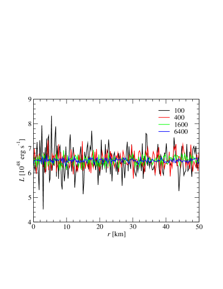
Figure 1.— The radial profile of the luminosity for a central point source emitting into a static scattering atmosphere for four different MC runs. In the first run (black line), we emit $100$ MCPs at each timestep, while in the second run we produce $400$ MCPs in a timestep, etc. In agreement with the analytical solution (cf. Section 9.1.1), the luminosity is constant along the radial coordinate within statistical errors. According to the central limit theorem and as demonstrated in Fig. 2, these errors decrease as $1/N^{1/2}$, where $N$ is the number of MCPs.

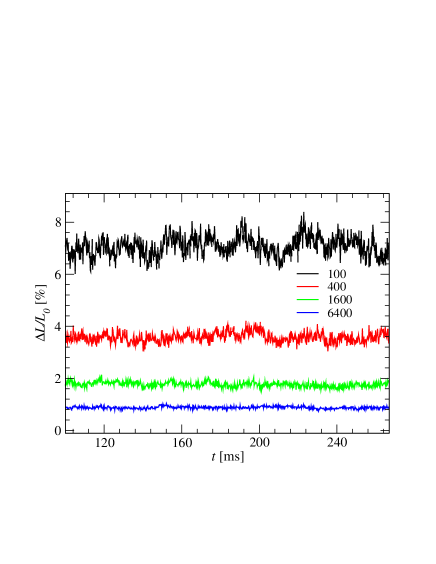
Figure 2.— Average deviation of the luminosity from its average value in each cell as a function of time for radiation from a central point source emitting into a static scattering atmosphere. The black line corresponds to a run in which we emit $100$ MCPs in each timestep, while the red line represents the run with $400$ MCPs, etc. In agreement with the central limit theorem, the average deviation decreases as $1/N^{1/2}$, where $N$ is the number of MCPs.

9.1.2 Homogeneous sphere

The homogeneous sphere problem is frequently employed to test radiative transfer codes (Bruenn, 1985; Schinder & Bludman, 1989; Smit et al., 1997; Rampp & Janka, 2002). This problem consists of a static homogeneous and isothermal sphere of radius $R$ that radiates into vacuum. Inside the sphere, the radiation interacts with the background matter only via isotropic absorption and thermal emission.

Despite its simplicity, the problem possesses some important physical and numerical properties that are often encountered in many practical applications: There is a sharp discontinuity at the surface of the sphere, and this represents a major challenge for finite-difference methods. However, Monte Carlo methods are well positioned for treating such discontinuities. Moreover, a situation similar to the stiff transition from the radiation diffusion regime inside an opaque sphere to a free-streaming regime in the ambient vacuum occurs near a PNS surface in core-collapse supernova simulations. Such a transition is a source of significant errors in approximate transport schemes such as, e.g., flux-limited diffusion (Ott et al., 2008).

We assume that the sphere of radius $R$ has a constant absorption opacity $\kappa_{a}$ and emissivity $B$ in the interior, while in the ambient vacuum at $r>R$, we have $\kappa_{a}=B=0$. For this problem, the transport equation can be solved analytically (Smit et al., 1997):

$$I(r,\mu)=B\left(1-e^{-\kappa_{a}s(r,\mu)}\right)\,,$$ (158)

where

$$s(r,\mu)=\left\{\begin{array}[]{ll}r\mu+Rg(r,\mu)&\mathrm{if}\ \ r<R,\quad-1\leq\mu\leq 1\,,\\ &\\ 2Rg(r,\mu)&\mathrm{if}\ \ r\geq R,\quad\sqrt{1-\left(\frac{R}{r}\right)^{2}}\leq\mu\leq 1\,.\\ &\\ 0&\mathrm{otherwise}\end{array}\right.$$ (159)

and

$$g(r,\mu)=\sqrt{1-\left(\frac{r}{R}\right)^{2}(1-\mu^{2})}\,.$$ (160)

Note that this solution depends only on three parameters: $\kappa_{a}$, $R$, and $B$, where the latter acts as a scale factor for the solution.

We perform a set of simulations with $R=10$ km, $\kappa_{a}=2.5\times 10^{-4}\ \mathrm{cm}^{-1}$ and $B=10$ (in CGS units). Our computational domain has an outer radius of $50$ km and is covered by $100$ equidistant cells. For this setup, we carry out three runs, in which we choose MCP weights such that $10^{5}$, $4\times 10^{5}$, or $1.6\times 10^{6}$ new MCPs are emitted in each timestep in a given simulation (hereafter, simulations A, B, and C). Figure 3 shows the zeroth moment $J$ as a function of the radial coordinate for simulations A, B, and C when the stationary-state radiation field is reached (black, red, and green lines, respectively). Also shown (blue line) is the zeroth moment $J$ from the analytical solution given by equations (158)-(160). As we can see, the Monte Carlo solution agrees well with the analytical solution within statistical errors. The inset plot in Fig. 3 shows the time evolution of the average deviation of the zeroth moment in the Monte Carlo solution from the analytical result when the stationary state is reached. The average deviation in simulations A, B, and C fluctuate around $\simeq 0.14$, $\simeq 0.27$, $\simeq 0.53$, respectively. Hence, in these simulations, when the number of MCPs is increased by a factor of $4$, the average deviation decreases by a factor of $\simeq 2$, in agreement with the central limit theorem, and the solution converges to the analytical result. We have repeated this simulation set with different values of $\kappa_{a}$, $B$, $R$ and different grid resolutions. In all cases, we find excellent agreement with the analytical result, similar to the case discussed above.

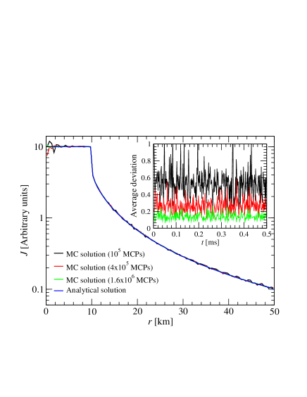
Figure 3.— The zeroth moment for radiation $J$ as a function of radial coordinate $r$ in the homogeneous sphere test for three simulations in which $10^{5}$, $4\times 10^{5}$, and $1.6\times 10^{6}$ new MCPs are emitted in each timestep (black, red, and green lines, respectively). Also shown (blue line) is the zeroth moment from the analytical solution. The inset plot shows the average deviation of the zeroth moment in these three Monte Carlo simulations from the analytical solution.

9.1.3 Diffusion of a Gaussian Pulse

In order to show that our code handles diffusion of radiation properly, we calculate the diffusion of a Gaussian radiation packet through static matter. We assume that radiation interacts with matter only via isotropic and isoenergetic scattering, and the scattering opacity $\kappa_{s}$ is assumed to be constant in space and time.

The diffusion of a Gaussian packet with initial central position at $r=r_{\mathrm{ini}}$ and width $d_{0}$ in such a medium is described by the following analytical solution (Swesty & Myra, 2009; Sumiyoshi & Yamada, 2012)

$$E(r,t)=E_{\mathrm{ini}}\left(\frac{t_{\mathrm{ini}}}{t_{\mathrm{ini}}+t}\right)^{\omega}\exp\left(\frac{-|r-r_{\mathrm{ini}}|^{2}}{4D(t_{\mathrm{ini}}+t)}\right)\,,$$ (161)

where $E(r,t)$ is the radiation energy density at position $r$ and time $t$ after initial time $t_{\mathrm{ini}}$. The diffusion coefficient, $D$, equals $c/3\kappa_{s}$ and the width of the Gaussian pulse, $d_{\mathrm{ini}}$, as a function of the initial time equals $(4Dt_{\mathrm{ini}})^{1/2}$. Parameter $E_{\mathrm{ini}}$ is the initial height of the packet and $\omega$ is related to the number of spatial dimensions, $N_{\mathrm{D}}$, and is equal to $N_{\mathrm{D}}/2$.

In our runs, we place the packet at the center of our computational domain with the radial coordinate extending up to $3\times 10^{7}$ cm ($300$ km). We choose the initial width of the packet to be $10^{6}$ cm, while the scattering opacity is set equal to $2\times 10^{-4}\ \mathrm{cm}^{-1}$. We run each simulation with the DDMC and MC schemes and use $2\times 10^{5}$ MCPs with constant weight in each of the runs. Figure 4 shows the radial profile of $E$ at three different times ($0$, $30$, and $60$ ms). The black line corresponds to the analytical solution, the dashed-red line is obtained from the DDMC run, and the dotted green line is the MC solution. Due to diffusion, the radial profile of radiation flattens with time. During the first $30$ ms of evolution, the central radiation energy density decreases be a factor of $\sim$20, while in the next $30$ ms it decreases further by a factor of $\sim$2. Therefore, the $60$ ms timescale captures the diffusion timescale of the problem. As we can see in the plot, both the DDMC and MC methods model diffusion of radiation in scattering medium quite well. The fluctuations around the analytic solution are due to the Monte Carlo treatment of transport in a scattering medium, and their magnitude again decreases as $N^{1/2}$. We have also repeated these runs with different values of the scattering opacity $\kappa_{s}$ and different widths, $d_{\mathrm{ini}}$, of the Gaussian, and we always find that both from DDMC and MC schemes agree with the analytical solution within statistical errors.

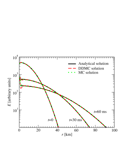
Figure 4.— The radial profile of the energy density of a Gaussian radiation packet diffusing into a uniform medium with a constant scattering opacity at three different times. The black line corresponds to the analytical solution, the dashed red line is obtained using the DDMC scheme, while the dotted green line is produced by the MC scheme. Note that the fluctuations in the energy density that are particularly visible near the central region at $t=30$ ms and $t=60$ ms are simply caused by the random noise intrinsic to Monte Carlo methods. This noise is particularly pronounced in central zones because those zones have smaller volumes and thus contain smaller numbers of MCPs. One can reduce this noise by choosing smaller weights for MCPs in central regions. In our test, we use constant weight everywhere for the entire radiation packet. Moreover, these fluctuation decrease with increasing number of MCPs, according to the central limit theorem.

9.2. Protoneutron star cooling

In this section, we consider the early cooling and deleptonization of a young non-rotating PNS formed in a CCSN. This problem is provided as a test of neutrino-matter coupling and as a testbed for optimal sampling methods and MCP weights. This particular problem was chosen because it is a realistic physical context similar to that for which our MC and DDMC algorithms were designed. The reader should note, however, that there is no analytic or agreed-upon benchmark solution for this problem and, therefore, that we are testing the behavior and speed of the solutions, not the numerical results themselves.

9.2.1 Numerical Setup

For our PNS model, we employ the post-core bounce configuration produced in the collapse of the s20.0 progenitor model of Woosley et al. (2002) with the 2D multi-group multi-angle simulations of Ott et al. (2008). We start with a background model at $160$ ms after bounce, and evolve it with our Monte Carlo code. In doing so, we first evolve the radiation field with fixed $T$ and $Y_{\mathrm{e}}$ until it reaches a steady state, after which we inaugurate coupling to $T$ and $Y_{\mathrm{e}}$. Our computational domain extends up to $300$ km, and is covered with 100 fixed logarithmically-spaced radial zones. The central zone has a width of $500$ m. The timestep is chosen to be the light-crossing time of the central zone. We assume that the PNS is static and neglect velocity-dependent effects.

We include the standard set of neutrino interactions listed in Thompson et al. (2003). We use $48$ logarithmically spaced energy groups from $2.5$ MeV to $250$ MeV to calculate the “leakage” opacities from one energy group to another due to inelastic scatterings in the DDMC region (however, the energies of MCPs are, of course, not discretized, since they are selected randomly using the local emissivity. See discussion in Section 7.1). Electron neutrinos and antineutrinos are treated independently, while we combine heavy-lepton neutrinos ($\nu_{\mu}$, $\bar{\nu}_{\mu}$, $\nu_{\tau}$, and $\bar{\nu}_{\tau}$) together into one group.

Sampling of Monte Carlo particles. We sample Monte Carlo particles in each spatial zone by calculating the number of neutrinos emitted in each zone during each timestep and then by choosing the weight of MCPs in each zone. We choose the weights of MCPs based on the following function

$$\left(\frac{{{\dot{T}}_{\mathrm{emis}}}}{T}\frac{{{\dot{Y}}_{\mathrm{e,emis}}}}{Y_{\mathrm{e}}}\right)^{0.5}\left(\frac{1}{\kappa_{\mathrm{p}}c}\right)^{h}\ ,$$ (162)

where $h$ is a constant parameter. Terms ${\dot{T}}_{\mathrm{emis}}$ and ${\dot{Y}}_{\mathrm{e,emis}}$ are the rates of change of $T$ and $Y_{\mathrm{e}}$ that would occur if there were only emission and no absorption. Term $\kappa_{\mathrm{p}}$ is the mean absorption opacity; hence, $1/\kappa_{\mathrm{p}}c$ represents a timescale for absorption of radiation. Therefore, the quantity in expression (162) is larger in regions that emit strongly with small absorption. Stated differently, this quantity should have larger values in those regions where $T$ and $Y_{\mathrm{e}}$ are likely to undergo significant changes due to emission and subsequent escape of radiation, implying that sampling based on quantity (162) places particular emphasize on accurate modeling of PNS cooling and deleptonization. We experimented with several values of $h$ and found that $h=0.5$ for electron neutrinos and antineutrinos and $h=0.3$ for $\mu/\tau$ neutrinos lead to fairly smooth sampling of MCPs, where the largest number of MCPs are concentrated in zones that are subject to the fastest changes in $T$ and $Y_{e}$. However, we did not perform further studies of sampling and we do not claim that the spatial sampling of MCPs based on expression (162) is the optimal choice for modeling PNS evolution.

The Interface between DDMC and pure Monte Carlo regions. Since neutrino absorption and scattering cross sections are strongly energy-dependent, it is important to take this into account in choosing the spatial location of the interface between the DDMC and pure MC regions. To accomplish this, we introduce energy groups and calculate optical depth for each energy group. We then determine the spatial location of the interface for an MCP with an energy within a given group in terms of the optical depth for that group. More specifically, if the optical depth for the energy group of a given MCP exceeds some threshold value, $\tau_{\mathrm{DDMC}}$, then we assume that this MCP is in the DDMC region. The parameter $\tau_{\mathrm{DDMC}}$ is assumed to have the same value for each energy group, meaning that the interface is located at different radii for different energy groups. In our simulations, we calculate the optical depth at each timestep and adjust the interface to its new location corresponding to the new values of optical depth. In our tests below, we consider several values of $\tau_{\mathrm{DDMC}}$ and explore which value represents an optimal choice for simulations of PNS evolution.

Treatment of effective scattering. As mentioned in Section 7, in the DDMC regime, we split the effective scattering opacity $\tilde{\sigma}_{es,j,k}$ into two parts, $a_{j,k}\tilde{\sigma}_{es,j,k}$ and $(1-a_{j,k})\tilde{\sigma}_{es,j,k}$, where $0\leq a_{j,k}\leq 1$, and restrict the first of these two to be elastic effective scattering, while the second one is free to be inelastic (as “effective-scattering” scattering would otherwise generally be). As we have discussed in Section 7, the presence of an extra elastic scattering source does not increase the cost of doing DDMC transport. Therefore, by assuming that an $a_{j,k}\tilde{\sigma}_{es,j,k}$ fraction of effective scattering is elastic (instead of being inelastic), our computational savings are proportional to $a_{j,k}$.

We find that it is convenient to determine the parameter $a_{j,k}$ in terms of the Fleck factor $f_{j}$ in the following way:

$$a_{j,k}=f_{j}^{\frac{\delta}{1-\delta}},$$ (163)

where $\delta$ is a constant ranging from $0$ to $1$. For $\delta=0$, all of effective scattering is treated as inelastic, while for $\delta=1$, all of it is treated as elastic. This prescription has the advantage that at low optical depth – where effective scattering does not dominate calculations – most effective scattering is treated as inelastic, while at high optical depth – where calculations would otherwise be dominated by inelastic effective scatterings – a significantly larger fraction is treated as elastic, which leads to huge savings in computation. In the following, we explore what values of $\delta$ are most suitable for simulations of PNS evolution.

9.2.2 Results

In this section, we first present the stationary-state radiation field results, after which we describe the subsequent fully time-dependent calculations with coupling to $T$ and $Y_{\mathrm{e}}$. For these simulations, unless otherwise noted, we use $\tau_{\mathrm{DDMC}}=6$, $\delta=0.38$ and $\alpha=1$, and employing $100,000$ MCPs to model newly-emitted particles at each timestep.

Stationary state. Figure 5 shows the radial profiles of the RMS neutrino energies for the three types of neutrinos. The solid lines are produced by our Monte Carlo code, while the dashed ones are from the $\mathrm{S_{N}}$ calculations of Ott et al. (2008). The RMS energies agree well in the inner $\sim 50$ km region, while for $r\gtrsim 50$ km, the $\mathrm{S_{N}}$ code produces RMS energies that are larger by up to $\simeq 4\%$. We believe that this difference stems from the truncation errors in the energy discretization of Ott et al. (2008) calculations, which employ only $16$ logarithmic energy groups, whereas in our MC cases, we do not use energy discretization in selecting MCP energies. The corresponding spectral energy distribution of the neutrino luminosity at $300$ km normalized by the total luminosity for each neutrino type is shown in Fig. 6, which again demonstrates a good agreement between our MC calculation and $\mathrm{S_{N}}$ calculations of Ott et al. (2008).

Figure 7 shows the radial profile of the mean inverse flux factors for the three types of neutrinos. The solid lines again represent the Monte Carlo results, while the dashed lines are from the $\mathrm{S_{N}}$ calculations of Ott et al. (2008). Overall, we again find good agreement between the two results. The only systematic difference that we observe is that the $\mathrm{S_{N}}$ code tends to yield inverse flux factors that are larger by $\sim$1 $\%$ than the corresponding MC data at radii $\gtrsim 200$ km. This is most likely caused by the ray-effects intrinsic to $\mathrm{S_{N}}$ schemes. Nevertheless, we find good overall agreement between our Monte Carlo and the $\mathrm{S_{N}}$ calculations of Ott et al. (2008) for this stationary-state radiation field.

Time-dependent calculations. Figure 8 shows the luminosities for the three different neutrino species as a function of time during the first $150$ ms of evolution of the PNS model after being mapped to our code. As expected, the luminosities for all types of neutrinos decrease gradually during the first $150$ ms of evolution. On a short timescale of one timestep, the luminosity undergoes significant fluctuations around its average value. These are expected and are due to the stochastic nature of MCP emission, absorption, and scattering processes. These fluctuations decrease significantly if averaged over longer timescales, such as the PNS light-crossing time, and are practically “invisible” on much longer timescales, such as the dynamical timescale of the PNS. Moreover, we find that these fluctuations again decrease as $\sim N^{-1/2}$, where $N$ is the number of MCPs.

Figure 9 shows the radial profile of the temperature (upper panel) and electron fraction (bottom panel) at the beginning ($t=0$) and at the end ($t=150$ ms) of our simulation. During the early evolution, the temperature decreases noticeably in the region $r\gtrsim 15$ km due to emission and diffusion of radiation. There is no significant change in $T$ and $Y_{\mathrm{e}}$ in the inner $r\lesssim 15$ km region as the radiation diffuses out on much longer timescales from that region. The electron fraction decreases in the region $r\lesssim 60$ km due to copious emission of electron neutrinos, while in the region $r\gtrsim 60$ km $Y_{\mathrm{e}}$ increases as a result of the absorption of those neutrinos.

Quality of energy and lepton number conservation. As discussed in Section 6.2, our IMC scheme for neutrinos does not make any approximations that violate energy or lepton number conservation. Therefore, energy and lepton number should be conserved up to machine precision in practical calculations using this scheme. In our calculations, we see that this is indeed the case, and both energy and lepton number in the system are conserved in each timestep to the ${\cal O}(10^{-14})$ precision of the machine.

Treatment of effective scattering. As we mentioned above, we use prescription (163) in order to treat effective scattering in a computationally efficient way in the DDMC region. We have performed simulations for different values of the parameter $\delta$, ranging from $1$ (where all effective scatterings are elastic) to $0.286$ (where a significant fraction of effective scatterings are inelastic). We find that there is no systematic difference in the PNS evolution for values of $\delta$ that are smaller than $\simeq 0.38$. For example, the total energy $E_{\mathrm{esc}}$ (or lepton number $Y_{\mathrm{l,esc}}$) of neutrinos that leave the system through the outer boundary in the first $150$ ms of evolution decreases monotonically by $\sim 2\%$ when decreasing $\delta$ from $1$ to $0.38$. Further decrease of $\delta$ results in non-systematic variation in both $E_{\mathrm{esc}}$ and $Y_{\mathrm{l,esc}}$ with relative error of only $\sim 0.1\%$, without any monotonic dependence on $\delta$. The origin of such variations is likely to be numerical errors and not our prescription for the treatment of effective scattering. This implies that condition (7.1) for the validity of our approximate treatment of effective scattering is fulfilled for $\delta\lesssim 0.38$ and violated otherwise. On the other hand, because the cost of simulations increases with decreasing $\delta$, it is desirable to use the largest allowed value of $\delta$. Therefore, we conclude that $\delta=0.38$ is an optimal choice for the treatment of effective scattering in the DDMC regime, at least in modeling the early phases of PNS evolution.

Note that this feature is independent of the number of dimensions. It should be applicable as long as we have a young PNS surrounded by a lower density envelope, i.e. in any CCSN scenario.

The interface between DDMC and pure Monte Carlo regions. Figure 10 shows the computational time to perform the first $500$ timesteps as a function of the parameter $\tau_{\mathrm{DDMC}}$. We have performed simulations using different values of $\tau_{\mathrm{DDMC}}$, ranging from $5$ up to $1280$. Since Monte Carlo calculations are more expensive than DDMC calculations, the computational time increases with $\tau_{\mathrm{DDMC}}$. For example, for $\tau_{\mathrm{DDMC}}=5$ the first $500$ timesteps are performed within $1469$ s, while for $\tau_{\mathrm{DDMC}}=1280$ this simulation took $20,480$ s. We have not performed simulations with higher values of $\tau_{\mathrm{DDMC}}$, since such simulations become quite expensive, implying that it is impractical to perform neutrino transport in the PNS using only the IMC scheme without combining it with the DDMC (or an alternate) scheme. Interestingly, for this setup, the computational cost of simulations does not differ much for values of $\tau_{\mathrm{DDMC}}$ smaller than $\simeq 100$. This is because the DDMC scheme yields the largest speed-up in regimes dominated by scattering. At optical depth of $\lesssim 100$ (where the Fleck factor $f$ is $\sim 1$), there is significant contribution from absorption, which leads to modest increase of the computational time as we increase $\tau_{\mathrm{DDMC}}$ from $5$ to $100$. At higher optical depths (where $f\sim 0$), effective scatterings start to dominate, which leads to steep increases of computational time with $\tau_{\mathrm{DDMC}}$.

From a theoretical point of view, the DDMC scheme is accurate if the underlying approximations – which are based on Fick’s law – are fulfilled to a sufficient degree in each zone. Fick’s law holds in a given zone if the mean-free-path of MCPs are significantly smaller than the grid size. If we assume that the grid size is of the order of $1$ km, then for a typical young PNS model, this requirement translates to $\tau_{\mathrm{DDMC}}\gtrsim 6$ (for a given energy group). Therefore, for $\tau_{\mathrm{DDMC}}\gtrsim 6$ we expect our DDMC scheme to yield sufficiently accurate results. Indeed, to verify this premise we have performed a series of long-evolution simulations for values of $\tau_{\mathrm{DDMC}}$ in a wide range. We find that the results (such as luminosity, etc.) indeed agree to within $\sim 1\%$ for any value of $\tau_{\mathrm{DDMC}}$ larger than $\sim 6$.

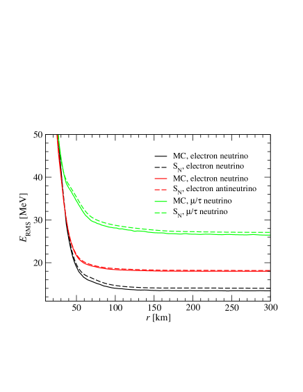
Figure 5.— The stationary state radial profiles of the RMS neutrino energies for the three different types of neutrinos obtained with our Monte Carlo scheme (solid lines). For comparison, we show results obtained by  Ott et al. (2008) with an $\mathrm{S_{N}}$ code (dashed lines).

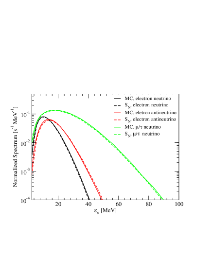
Figure 6.— The stationary state neutrino spectra at 300 km normalized by the total luminosity obtained with our Monte Carlo scheme (solid lines). For comparison, we show results obtained by  Ott et al. (2008) with an $\mathrm{S_{N}}$ code (dashed lines).

Figure 7.— The stationary state radial profiles of the mean inverse flux factors for the three different types of neutrinos obtained with our Monte Carlo scheme (solid lines). For comparison, we show results obtained by  Ott et al. (2008) with an $\mathrm{S_{N}}$ code (dashed lines).

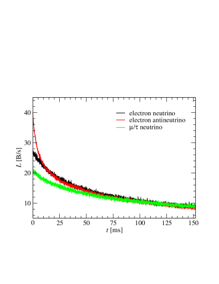
Figure 8.— Luminosity as a function of time in our PNS evolution calculation.

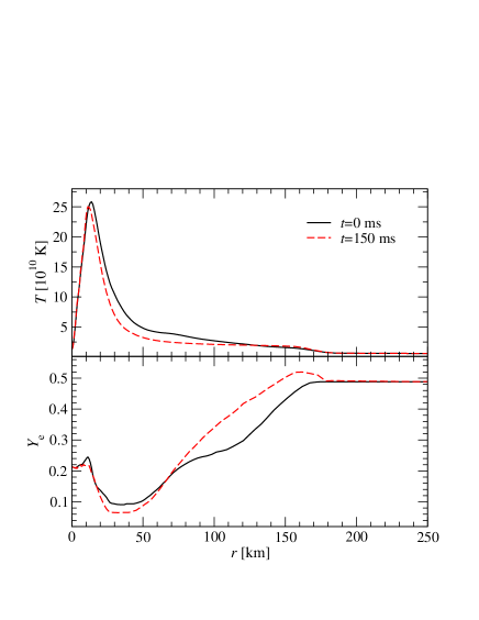
Figure 9.— The radial profiles of the temperature $T$ and electron fraction $Y_{e}$ at $t=0$ and $t=150$ ms after the start of simulation.

Figure 10.— Time spent for performing first 500 timesteps as a function of parameter $\tau_{\mathrm{DDMC}}$ for PNS evolution simulations. Since at high optical depth the pure Monte Carlo calculations are more expensive than the DDMC calculations, the computational time increases with $\tau_{\mathrm{DDMC}}$. Beyond $\tau_{\mathrm{DDMC}}>1280$, our simulations become computationally too expensive, and we do not consider even larger values of $\tau_{\mathrm{DDMC}}$.

The importance of the implicit scheme. The simulations presented in this section are performed using the implicit Monte Carlo scheme with a “most implicit” choice of $\alpha=1$ within the framework of the IMC (cf. equation 60). We repeated some of the runs with the “less implicit” value of $\alpha=0.5$, which results in a Fleck factor that is larger by a factor of $\sim 2$ than in the $\alpha=1$ case in the diffusive regime (cf. equation 63). This results in a slight decrease in solution accuracy, but we do not observe any instabilities. One obvious question to ask is: would it be possible to perform the same simulations with an explicit treatment of the emissivity? The answer is clearly no. With the current timestep set by the light crossing time for the central zone of width $500$ m, the fully explicit scheme crashes within a few timesteps. For it to be stable, one would have to use timesteps of the order of the smallest mean-free-path, which can be as small as $\lesssim 1$ m in the center of the PNS. Hence, in order to use a time-explicit scheme, we would need to decrease our timestep by a factor of at least $\sim 500$, which would make useful simulations completely impractical. For the above choice of parameters (i.e., $\tau_{\mathrm{DDMC}}=6$, $\delta=0.38$ and $\alpha=1$, and employ $100,000$ MCPs to model newly emitted particles at each timestep), the computational cost of performing the first $150$ ms of PNS evolution is about $36$ hours on $96$ cores on the Hopper Cray XTE6 cluster at NERSC.

Parallel scaling. In order to study parallel scaling of our code, we perform simulations on a number of cores ranging from $24$ up to $1152$ on the Hopper Cray XTE6 cluster at NERSC. We implement hybrid OpenMP/MPI parallelization and use 6 OpenMP threads per each MPI process in our tests.

Figure 11 shows the time spent per MPI process $t_{\mathrm{mpi}}$ as a function of the number of cores $N_{\mathrm{core}}$ in our weak scaling test. In this test, we increase the number of MCPs proportionally to the number of MPI processes, while other problem parameters remain fixed. Here, the amount of computational work is chosen in such a way that the time on $24$ cores is equal to $1$ s. This time increases slowly with $N_{\mathrm{core}}$ and reaches $1.35$ s for $N_{\mathrm{core}}=1152$, a value that is only $35\%$ larger than the one for $24$ cores.

The inset plot of Fig. 11 shows the total simulation time as a function of the number of cores in our strong scaling test. The simulation time decreases almost linearly (in logarithmic scale) with $N_{\mathrm{core}}$ and reaches $1.53$ s at $N_{\mathrm{core}}=1152$. This number is only $70\%$ larger than the time corresponding to ideal scaling. Based on these results, we conclude that our code scales nicely up to $1152$ cores, which is more than sufficient for 1D problems.

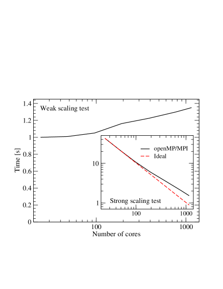
Figure 11.— The simulation time as a function of the number of cores in our strong (main plot) and weak (inset plot) scaling tests. In both plots, the $x$-axes show the number of cores, while the $y$-axes are the simulations times [in seconds]. The solid black lines show the simulation time using our code, while the dashed red line in the inset plot corresponds to ideal strong scaling.

9.3. Moving background with fixed $T$ and $Y_{e}$

In this section we describe a test problem that involves the propagation of radiation in moving matter to demonstrate the ability of our code to perform transport in a moving medium. In this test, we neglect the change in temperature ($T$) and electron fraction ($Y_{e}$) of matter due to emission, absorption, or scattering of radiation.

9.3.1 Homologously expanding shell

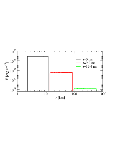
Figure 12.— The radial profile of the radiation energy density measured by a comoving observer at different times in the homologously expanding shell test for simulation A1D using $1,280,000$ MC particles. See the discussion in the main text for further details of the simulation.

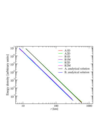
Figure 13.— The radiation energy density in the comoving frame as a function of the radial coordinate inside homologously expanding shell

A spherically-symmetric shell of matter, in which radiation is trapped, is expanding self-similarly with velocity $V_{r}\propto r$. For simplicity, we assume that matter interacts with radiation only through elastic scattering, without any emission or absorption. According to the analytical solution (Mihalas & Mihalas, 1984), the average energy of neutrinos $\langle\varepsilon_{\nu}\rangle$ in the expanding shell should decrease as

$$\langle\varepsilon_{\nu}\rangle\propto\frac{1}{r}$$ (164)

due to the Doppler shift, while the radiation energy density $E_{0}$ should decrease according to

$$E_{0}\propto r^{-4}\,,$$ (165)

due to both the Doppler shift and expansion of the shell.

We perform two sets of test simulations. In the first set, we use a very large constant value of the scattering opacity $\kappa_{s}$ of $5\cdot 10^{3}\ \mathrm{cm}^{-1}$, while in the second set, we use a million times smaller value of $5\cdot 10^{-3}\ \mathrm{cm}^{-1}$. The reason for choosing two such sets is the following. Generally speaking, for such tests, it is desirable to have as large an opacity as possible in order to avoid diffusion of radiation out of the expanding shell, which can lead to the violation of relation (165). However, the high computational cost of performing MC transport at high scattering opacity limits the maximum value of $\kappa_{s}$ that we can simulate. On the other hand, the DDMC scheme is particularly efficient in the regime dominated by elastic scattering (see the discussion in Section 7). Therefore, we perform simulations with $\kappa_{s}=5\times 10^{3}\ \mathrm{cm}^{-1}$ using only the DDMC scheme, after which we do a set of runs with $\kappa_{s}=5\times 10^{-3}\ \mathrm{cm}^{-1}$ using both the DDMC and MC schemes. In the former case, the radiation is completely trapped in the matter, and there is no diffusion of MCPs from one cell to another during the simulated time. Instead, the MCPs are transported due only to velocity-dependent effects caused by the expansion of the shell. Moreover, in this case, the random numbers are used only for initial sampling of MCPs, while the velocity-dependent (operator-split) part of the transport is completely deterministic (see the discussion in Section 8.2). Therefore, in this set of runs, we exclusively test the ability of our DDMC scheme to treat velocity-dependent effects. In the second set of test runs, since we use a smaller value of the scattering opacity, the result is affected also by diffusion of MCPs from the expanding shell. This is prone to statistical errors arising from the DDMC treatment of diffusion. Hence, in this case, we explore the ability of the code to perform transport of radiation in moving matter when the transport process itself is affected by statistical errors.

In both sets of test runs, our shell initially has a radial extent ranging from $r_{\mathrm{min}}=2.25$ km to $r_{\mathrm{max}}=12.25$ km. We assume that the radiation initially has a constant energy density profile. The shell velocity is given by $v_{r}=\varpi cr/R_{\mathrm{out}}$, where $\varpi$ is a constant, $c$ is the speed of light, $r$ is the radial coordinate, and $R_{\mathrm{out}}$ is the radius of the outer boundary of our computational domain. Our entire domain is covered by $1200$ radial cells with constant size. In these simulations, we choose $\varpi$ to be $0.4$ and $0.8$, while $R_{\mathrm{out}}$ is chosen to be $600$ km. For the first set of test runs, we perform 4 simulations with $40,000$, $64,000$ $256,000$, $1,280,000$ MC particles for each of the two values of parameter $\varpi$. For the second set, we perform 3 simulations with $10,000$, $40,000$, and $164,000$ MCPs for each value of $\varpi$ using the MC and DDMC schemes. We use the following naming convention for our test simulations: the names of the first set of runs start with “A,” while the second set starts with “B.” The second symbol represents the value of $\varpi$ (“1” for $\varpi=0.4$ and “2” for $\varpi=0.8$), while the last letter indicates whether we use the DDMC or MC scheme (“D” for DDMC and “M” for MC). Thus, for example, the DDMC run with $\varpi=0.4$ from the first set is denoted as A1D, while the similar run with $\varpi=0.8$ is called A1D.

Figure 12 shows the radiation energy density in the comoving frame in each radial cell as a function of the radial coordinate of those cells at $0$ ms (black line), $9.2$ ms (red line), and $19.4$ ms (green line) after the start of shell expansion for model A1D. During this evolution, the radial extent of the shell increases by a factor of $\sim\!50$, which leads to a decrease in radiation energy density by a factor of $\sim\!5\times 10^{6}$. Due to homologous nature of the expansion, the radial profile of the energy density should stay constant. As we can see in the plot, our code indeed reproduces its constant radial profile within statistical errors. These statistical errors are caused by the initial pseudo-random sampling of MCP positions and energies, and their magnitude decreases as we increase the number of MCPs.

Figure 13 shows the average energy density in several outermost zones as a function of the mean radial coordinate of those zones for simulations A1D and A2D using $1,280,000$ MCPs (red and green lines, respectively). The outermost zones are expanding with the fastest velocity compared to the other parts of the shell and, thus, are affected by the velocity-dependent effects to the greatest degree. This plot also shows energy as a function of $r$ according to the analytical solution (black line). As we see, the result of these simulations agrees well with the analytical result during the simulated time.

Figure 13 also shows the energy density in several central zones of the expanding shell as a function of the mean radial coordinate of those zones for the second set of test runs. Here we focus on the central zones (instead of the outermost zones, as we did for the models of the first set) because the scattering opacity in these runs is relatively small. Thus, some fraction of the trapped radiation diffuses out of the shell during expansion. The behavior of radiation in the central zones is affected by this diffusion to a much smaller degree compared to that in the outer zones. This plot also shows the energy density versus the radial coordinate from the analytical solution (red line). As we see, both the MC and DDMC schemes agree with the analytical result within the statistical errors during the simulated time. These statistical errors again decrease as we increase the number of MCPs.

10. Conclusion and Future Work

We have generalized the implicit Monte Carlo (IMC) scheme of Fleck & Cummings (1971) and the discrete-diffusion Monte Carlo (DDMC) method of Densmore et al. (2007) to energy- and velocity-dependent neutrino transport. While the IMC method provides a stable and accurate time discretization of the transport equation, the DDMC method increases the computational efficiency of IMC at high optical depths using the diffusion approximation (as is appropriate).

In the IMC method for photons, one uses the matter energy equation in order to derive a time discretization of the transport equation in which the emissivity term is treated semi-implicitly. Since neutrino emissivity depends not only on energy, but also on the electron fraction, in order to derive the IMC equations for neutrinos with lepton number coupling, one has to use not only the energy equation, but also an equation for the evolution of the electron fraction $Y_{\mathrm{e}}$. Similar to the photon case, the IMC neutrino transport equation has new terms that formally describe scattering of radiation. In the Monte Carlo interpretation of the IMC equation, these scatterings model a fraction of the absorption and subsequent re-emission of radiation within a timestep and are called effective scatterings. Such scattering effectively decreases the energy exchanged between matter and radiation within a timestep and makes the scheme unconditionally stable. However, unlike in the photon case, the IMC scheme for neutrinos has two types of effective scatterings: one in which the total energy is conserved (as in photon IMC), and another for which the total lepton number is conserved during effective scattering (this scattering type does not exist in photon IMC; see the discussion in Section 6).

In extending the gray DDMC scheme of Densmore et al. (2007) to the energy-dependent case, we not only added discretization in particle energy, but also proposed a new (approximate) way of treating effective scattering in the DDMC regime to achieve additional speed up. We split the total effective scattering opacity into two parts, and the first part is treated as inelastic (as it would otherwise be), while the other part is treated as elastic. This leads to extra savings in computational cost because DDMC does not need to perform any additional operations to model elastic scatterings (Section 7). We parametrize the fraction of the effective scattering treated as elastic in terms of a new variable $\delta$ and show that for $\delta\simeq 0.38$, this approximation is excellent for modeling neutrino transport in systems that consist of a newly-born PNS with a hot, tenuous surrounding medium.

Furthermore, we have extended the above schemes to include velocity-dependence. In the pure (i.e., non-DDMC) Monte Carlo regime, we use the mixed-frame formalism (Mihalas & Klein, 1982; Hubeny & Burrows, 2007) in which emissivities and opacities are defined in the comoving frame, while transport is performed in the lab frame. This is easy to implement and allows one to take into account velocity-dependent effects correctly for arbitrarily large (relativistic) fluid velocities, provided that the spatial resolution and timestep are appropriate for capturing the motion of the fluid in each cell. In the DDMC regime, we use a somewhat different approach. Since the diffusion equation is formulated most naturally in the comoving frame, we start with the equation for the comoving zeroth moment of radiation accurate to ${\cal O}(V/c)$, and split it into three equations that are then solved in operator-split manner. One part deals with diffusion of radiation, the second part models advection and compression/decompression of radiation, while the third one takes into account the Doppler shift of radiation energy. The first equation is identical to the DDMC equations in the zero-velocity case and, thus, is solved in exactly the same way, while the second and third parts can be incorporated using simple operations (Section 8.2).

In order to test and validate these schemes, we have implemented them in our 1D spherically-symmetric code and applied it to several test problems. In particular, by considering an early evolution of a young PNS, we show that the IMC method allows much larger timesteps than what would be possible with a fully time-explicit scheme (Section 9.2). Moreover, the DDMC scheme leads to huge saving in computational cost due to the more efficient treatment of transport at high optical depth. Therefore, in our scheme, we use the DDMC method in regions with sufficiently high optical depth, while in the remaining part, we employ the pure IMC method. We find that the cost of performing a PNS evolution with the pure IMC scheme is usually orders of magnitude higher than the cost with a combination of the IMC and DDMC schemes (cf. Fig. 10). All in all, we conclude that the combination of the IMC and DDMC approaches represents a robust and accurate method for neutrino transport in core-collapse supernovae.

Finally, we point out that our energy- and velocity-dependent scheme can also be used for photon transport with minimal modifications. The only changes needed are disabling $Y_{e}$ changes and swapping in opacities and emissivities corresponding to photons.

Having developed a velocity-dependent transport algorithm, our next task is to couple it to hydrodynamics. Furthermore, in the future, we plan to generalize our code to the two- and three-dimensional cases and to extend it to general relativity.

11. Acknowledgments

We are happy to acknowledge helpful exchanges with Timothy Brandt, Jeffery Densmore, Peter Diener, Roland Haas, Daniel Kasen, Oleg Korobkin, and Christian Reisswig. This work was supported in part by NSF under grant nos. AST-0855535, OCI-0905046, OCI 0721915, OCI 0725070, OCI 0905046, OCI 0941653, PIF-0904015, PHY-0960291, and TG-PHY100033, by the DOE under grant DE-FG02-08ER41544, and by the Sherman Fairchild Foundation. Results presented in this article were obtained through computations on machines of the Louisiana Optical Network Initiative under grant loni_numrel07, on the Caltech compute cluster “Zwicky” (NSF MRI award No. PHY-0960291), on the NSF Teragrid under grant TG-PHY100033, and at the National Energy Research Scientific Computing Center (NERSC), which is supported by the Office of Science of the US Department of Energy under contract DE-AC03-76SF00098.

Appendix A Calculation of $\partial U_{r}/\partial T$ and $\partial U_{r}/\partial Y_{e}$ using the Fermi-Dirac function

Here, we derive analytical expressions for the equilibrium energy density of neutrinos $U_{r}$ and its partial derivatives with respect to $T$ and $Y_{e}$ using the expression for the Fermi-Dirac function $B(\varepsilon,T,Y_{e})$. The Fermi-Dirac function for neutrinos has the following form:

$$B(\varepsilon,T,Y_{e})=\frac{\varepsilon^{3}}{(hc)^{3}}\frac{1}{\exp\left[\frac{\varepsilon}{kT}-\eta(T,Y_{e})\right]+1}\,,$$ (A1)

where $\eta$ is the degeneracy parameter, which equals to $(\mu_{e}-\mu_{n}+\mu_{p})/{kT}$, $-(\mu_{e}-\mu_{n}+\mu_{p})/{kT}$, and $0$ for electron neutrinos, electron anti-neutrinos, and heavy lepton neutrinos, respectively, Here, $\mu_{e}$, $\mu_{n}$ and $\mu_{p}$ are the chemical potentials of the electron, neutron, and proton. Using the definition of the equilibrium energy density of neutrinos $U_{r}$ given by equation (25), we obtain:

$$\frac{\partial U_{r}}{\partial T} = \frac{4\pi}{c}\int_{0}^{\infty}\frac{\partial B}{\partial T}\,d\varepsilon\,,$$ (A2)

$$\frac{\partial U_{r}}{\partial Y_{e}} = \frac{4\pi}{c}\int_{0}^{\infty}\frac{\partial B}{\partial Y_{e}}\,d\varepsilon\,,$$ (A3)

where functions $\frac{\partial B}{\partial T}$ and $\frac{\partial B}{\partial Y_{e}}$, can be obtained using formula (A1):

$$\frac{\partial B}{\partial T} = \frac{B\exp\left(\frac{\varepsilon}{kT}-\eta\right)}{\exp\left(\frac{\varepsilon}{kT}-\eta\right)+1}\left[\frac{\varepsilon}{kT^{2}}+\left(\frac{\partial\eta}{\partial T}\right)_{Y_{e},\rho}\right]\,,$$ (A4)

$$\frac{\partial B}{\partial Y_{e}} = \frac{B\exp\left(\frac{\varepsilon}{kT}-\eta\right)}{\exp\left(\frac{\varepsilon}{kT}-\eta\right)+1}\left(\frac{\partial\eta}{\partial Y_{e}}\right)_{T,\rho}\,.$$ (A5)

Functions $d\eta/dT$ and $d\eta/dY_{e}$ are expressed in terms of the derivatives of $\mu_{e}$, $\mu_{n}$, and $\mu_{p}$ that can be calculated using EOS tables. Finally, the integrals in equation (A2) can be evaluated numerically, or can be expressed in terms of the Fermi integrals. The latter can be calculated either via direct numerical integration or by using a series expansion (Takahashi et al., 1978).

References

- Adams & Larsen (2002) Adams, M. L., & Larsen, E. W. 2002, Progress in Nuclear Energy, 40, 3
- Bethe (1990) Bethe, H. A. 1990, Reviews of Modern Physics, 62, 801
- Bruenn (1985) Bruenn, S. W. 1985, ApJS, 58, 771
- Bruenn et al. (2006) Bruenn, S. W., Dirk, C. J., Mezzacappa, A., Hayes, J. C., Blondin, J. M., Hix, W. R., & Messer, O. E. B. 2006, Journal of Physics Conference Series, 46, 393
- Bruenn et al. (2009) Bruenn, S. W., Mezzacappa, A., Hix, W. R., Blondin, J. M., Marronetti, P., Messer, O. E. B., Dirk, C. J., & Yoshida, S. 2009, Journal of Physics Conference Series, 180, 012018
- Brunner & Brantley (2009) Brunner, T. A., & Brantley, P. S. 2009, J. Comput. Phys., 228, 3882
- Brunner et al. (2006) Brunner, T. A., Urbatsch, T. J., Evans, T. M., & Gentile, N. A. 2006, J. Comput. Phys., 212, 527
- Buras et al. (2006a) Buras, R., Janka, H.-T., Rampp, M., & Kifonidis, K. 2006a, A&A, 457, 281
- Buras et al. (2006b) Buras, R., Rampp, M., Janka, H.-T., & Kifonidis, K. 2006b, A&A, 447, 1049
- Burrows et al. (2007a) Burrows, A., Dessart, L., & Livne, E. 2007a, in American Institute of Physics Conference Series, Vol. 937, Supernova 1987A: 20 Years After: Supernovae and Gamma-Ray Bursters, ed. S. Immler, K. Weiler, & R. McCray, 370
- Burrows & Fryxell (1992) Burrows, A., & Fryxell, B. A. 1992, Science, 258, 430
- Burrows & Goshy (1993) Burrows, A., & Goshy, J. 1993, ApJ, 416, L75
- Burrows et al. (1995) Burrows, A., Hayes, J., & Fryxell, B. A. 1995, ApJ, 450, 830
- Burrows et al. (2006) Burrows, A., Livne, E., Dessart, L., Ott, C. D., & Murphy, J. 2006, ApJ, 640, 878
- Burrows et al. (2007b) —. 2007b, ApJ, 655, 416
- Burrows et al. (2000) Burrows, A., Young, T., Pinto, P., Eastman, R., & Thompson, T. A. 2000, ApJ, 539, 865
- Castor (2004) Castor, J. I. 2004, Radiation Hydrodynamics, ed. Castor, J. I. (Cambridge University Press, Cambridge, UK)
- Demorest et al. (2010) Demorest, P. B., Pennucci, T., Ransom, S. M., Roberts, M. S. E., & Hessels, J. W. T. 2010, Nature, 467, 1081
- Densmore & Larsen (2004) Densmore, J. D., & Larsen, E. W. 2004, J. Comput. Phys., 199, 175
- Densmore et al. (2007) Densmore, J. D., Urbatsch, T. J., Evans, T. M., & Buksas, M. W. 2007, J. Comput. Phys., 222, 485
- Fleck & Canfield (1984) Fleck, Jr., J. A., & Canfield, E. H. 1984, J. Comput. Phys., 54, 508
- Fleck & Cummings (1971) Fleck, Jr., J. A., & Cummings, Jr., J. D. 1971, J. Comput. Phys., 8, 313
- Gentile (2001) Gentile, N. A. 2001, J. Comput. Phys., 172, 543
- Gentile (2009) Gentile, N. A. 2009, in In Proc. International Conference on Mathematics, Computational Methods & Reactor Physics (M & C 2009), Vol. May 3-7, 2009 (American Nuclear Society, LaGrange Park, IL), 1170
- Godoy & Liu (2012) Godoy, W. F., & Liu, X. 2012, Journal of Computational Physics, 231, 4257
- Goodale et al. (2003) Goodale, T., Allen, G., Lanfermann, G., Massó, J., Radke, T., Seidel, E., & Shalf, J. 2003, in Vector and Parallel Processing – VECPAR’2002, 5th International Conference, Lecture Notes in Computer Science (Berlin: Springer)
- Habetler & Matkowsky (1975) Habetler, G. J., & Matkowsky, B. J. 1975, J. Math. Phys., 16, 856
- Hanke et al. (2011) Hanke, F., Marek, A., Mueller, B., & Janka, H.-T. 2011, ArXiv e-prints
- Herant et al. (1992) Herant, M., Benz, W., & Colgate, S. 1992, ApJ, 395, 642
- Herant et al. (1994) Herant, M., Benz, W., Hix, W. R., Fryer, C. L., & Colgate, S. A. 1994, ApJ, 435, 339
- Hillebrandt & Wolff (1985) Hillebrandt, W., & Wolff, R. G. 1985, in Nucleosynthesis: Challenges and New Developments, ed. W. D. Arnett and J. W. Truran (Chicago, IL: Univ. Chicago, Press), 131
- Hubeny & Burrows (2007) Hubeny, I., & Burrows, A. 2007, ApJ, 659, 1458
- Hummer & Rybicki (1971) Hummer, D. G., & Rybicki, G. B. 1971, MNRAS, 152, 1
- Janka (1991) Janka, H.-T. 1991, A&A, 244, 378
- Janka (1992) —. 1992, A&A, 256, 452
- Janka (2001) —. 2001, A&A, 368, 527
- Janka & Hillebrandt (1989) Janka, H.-T., & Hillebrandt, W. 1989, A&AS, 78, 375
- Janka & Mueller (1996) Janka, H.-T., & Mueller, E. 1996, A&A, 306, 167
- Kalos & Whitlock (2008) Kalos, M. H., & Whitlock, P. A. 2008, Monte Carlo Methods: Second Revised and Enlarged Edition, ed. Kalos, M. H. & Whitlock, P. A. (Wiley-VCH Verlag)
- Kasen et al. (2011) Kasen, D., Woosley, S. E., & Heger, A. 2011, ApJ, 734, 102
- Keil et al. (2003) Keil, M. T., Raffelt, G. G., & Janka, H.-T. 2003, ApJ, 590, 971
- Kitaura et al. (2006) Kitaura, F. S., Janka, H.-T., & Hillebrandt, W. 2006, A&A, 450, 345
- Larsen & Mercier (1987) Larsen, E. W., & Mercier, B. 1987, J. Comput. Phys., 71, 50
- Lattimer & Swesty (1991) Lattimer, J. M., & Swesty, F. D. 1991, Nucl. Phys. A, 535, 331
- Liebendörfer et al. (2004) Liebendörfer, M., Messer, O. E. B., Mezzacappa, A., Bruenn, S. W., Cardall, C. Y., & Thielemann, F.-K. 2004, ApJS, 150, 263
- Liebendörfer et al. (2001) Liebendörfer, M., Mezzacappa, A., Thielemann, F.-K., Messer, O. E., Hix, W. R., & Bruenn, S. W. 2001, Phys. Rev. D, 63, 103004
- Liebendörfer et al. (2005) Liebendörfer, M., Rampp, M., Janka, H.-T., & Mezzacappa, A. 2005, ApJ, 620, 840
- Marek & Janka (2009) Marek, A., & Janka, H.-T. 2009, ApJ, 694, 664
- Martin & Brown (2001) Martin, W. R., & Brown, F. B. 2001, Trans. Amer. Nucl. Soc., 85, 329
- McClarren & Hauck (2010) McClarren, R. G., & Hauck, C. D. 2010, Journal of Computational Physics, 229, 5597
- McClarren et al. (2008) McClarren, R. G., Holloway, J. P., & Brunner, T. A. 2008, J. Comput. Phys., 227, 2864
- McClarren & Urbatsch (2009) McClarren, R. G., & Urbatsch, T. J. 2009, J. Comput. Phys., 228, 5669
- Mezzacappa & Bruenn (1993) Mezzacappa, A., & Bruenn, S. W. 1993, ApJ, 410, 740
- Mezzacappa et al. (2007) Mezzacappa, A., Bruenn, S. W., Blondin, J. M., Hix, W. R., & Bronson Messer, O. E. 2007, in American Institute of Physics Conference Series, Vol. 924, The Multicolored Landscape of Compact Objects and Their Explosive Origins, ed. T. di Salvo, G. L. Israel, L. Piersant, L. Burderi, G. Matt, A. Tornambe, & M. T. Menna, 234
- Mihalas & Klein (1982) Mihalas, D., & Klein, R. I. 1982, J. Comput. Phys., 46, 97
- Mihalas & Mihalas (1984) Mihalas, D., & Mihalas, B. W. 1984, Foundations of radiation hydrodynamics, ed. Mihalas, D. & Mihalas, B. W. (New York, Oxford University Press)
- Morel et al. (2003) Morel, J. E., Wareing, T. A., Lowrie, R. B., & Parsons, D. K. 2003, Nucl. Sci. Eng., 144, 1
- Murphy & Burrows (2008) Murphy, J. W., & Burrows, A. 2008, ApJ, 688, 1159
- N’Kaoua (1991) N’Kaoua, T. 1991, SIAM J. Sci. and Stat. Comput., 12, 505
- Nomoto & Hashimoto (1988) Nomoto, K., & Hashimoto, M.-A. 1988, Phys. Rep., 163, 13
- Nordhaus et al. (2010) Nordhaus, J., Burrows, A., Almgren, A., & Bell, J. 2010, ApJ, 720, 694
- Ott et al. (2008) Ott, C. D., Burrows, A., Dessart, L., & Livne, E. 2008, ApJ, 685, 1069
- Pejcha & Thompson (2012) Pejcha, O., & Thompson, T. A. 2012, ApJ, 746, 106
- Pomraning (1973) Pomraning, G. C. 1973, The equations of radiation hydrodynamics, ed. Pomraning, G. C.
- Rampp & Janka (2000) Rampp, M., & Janka, H.-T. 2000, ApJ, 539, L33
- Rampp & Janka (2002) —. 2002, A&A, 396, 361
- Schinder & Bludman (1989) Schinder, P. J., & Bludman, S. A. 1989, ApJ, 346, 350
- Smit et al. (1997) Smit, J. M., Cernohorsky, J., & Dullemond, C. P. 1997, A&A, 325, 203
- Sumiyoshi & Yamada (2012) Sumiyoshi, K., & Yamada, S. 2012, ApJS, 199, 17
- Sumiyoshi et al. (2005) Sumiyoshi, K., Yamada, S., Suzuki, H., Shen, H., Chiba, S., & Toki, H. 2005, ApJ, 629, 922
- Suwa et al. (2010) Suwa, Y., Kotake, K., Takiwaki, T., Whitehouse, S. C., Liebendörfer, M., & Sato, K. 2010, PASJ, 62, L49
- Swesty (2006) Swesty, F. D. 2006, in Computational Methods in Transport, ed. F. Graziani (Springer), 469–486
- Swesty & Myra (2009) Swesty, F. D., & Myra, E. S. 2009, ApJS, 181, 1
- Takahashi et al. (1978) Takahashi, K., El Eid, M. F., & Hillebrandt, W. 1978, A&A, 67, 185
- Takiwaki et al. (2012) Takiwaki, T., Kotake, K., & Suwa, Y. 2012, ApJ, 749, 98
- Thomas (1930) Thomas, L. H. 1930, Quart. J. Math., 1, 239
- Thompson et al. (2003) Thompson, T. A., Burrows, A., & Pinto, P. A. 2003, ApJ, 592, 434
- Thompson et al. (2005) Thompson, T. A., Quataert, E., & Burrows, A. 2005, ApJ, 620, 861
- Tubbs (1978) Tubbs, D. L. 1978, ApJS, 37, 287
- Wollaber (2008) Wollaber, A. B. 2008, PhD thesis, University of Michigan
- Wollaber & Larsen (2009) Wollaber, A. B., & Larsen, E. W. 2009, in In Proc. International Conference on Mathematics, Computational Methods & Reactor Physics (M & C 2009), Vol. May 3-7, 2009 (American Nuclear Society, LaGrange Park, IL), 1170–1179
- Woosley et al. (2002) Woosley, S. E., Heger, A., & Weaver, T. A. 2002, Rev. Mod. Phys., 74, 1015
- Yakunin et al. (2010) Yakunin, K. N., et al. 2010, Classical and Quantum Gravity, 27, 194005
- Yamada et al. (1999) Yamada, S., Janka, H.-T., & Suzuki, H. 1999, A&A, 344, 533
- Zink (2008) Zink, B. 2008, ArXiv e-prints, 0810.5349