BitPath – Label Order Constrained Reachability Queries over Large Graphs

Abstract

In this paper we focus on the following constrained reachability problem over edge-labeled graphs like RDF – given source node x, destination node y, and a sequence of edge labels (a, b, c, d), is there a path between the two nodes such that the edge labels on the path satisfy a regular expression “*a.*b.*c.*d.*”. A “*” before “a” allows any other edge label to appear on the path before edge “a”. “a.*” forces at least one edge with label “a”. “.*” after “a” allows zero or more edge labels after “a” and before “b”. Our query processing algorithm uses simple divide-and-conquer and greedy pruning procedures to limit the search space. However, our graph indexing technique – based on compressed bit-vectors – allows indexing large graphs which otherwise would have been infeasible. We have evaluated our approach on graphs with more than 22 million edges and 6 million nodes – much larger compared to the datasets used in the contemporary work on path queries.

1 Introduction

With the advent of Semantic Web and RDF, graphs have become richer where edge labels represent the type of relationship between two nodes which are connected by that edge. Exploring paths in the graphs has been a well studied problem. Typically a path query problem either simply asks for existence of any path between two non-adjacent nodes in the graph (reachability queries), or provides a regular expression for the path, and asks for all pairs of nodes that have at least one path between them which satisfies the given regular expression (regular path queries). Constrained reachability queries ask if the given destination node is reachable from the source node through a path which satisfies the constraints given in the query. The definition of constraints depends on the targeted problem, e.g., number of hops, type of edge labels, or a regular expression etc. Constrained reachability queries find their applications in a variety of graph databases. Application of label-constrained-reachability (LCR) queries have been outlined by Jin et al. in [16]. In our work, we have focused on a different type of constrained reachability problem – label-order-constrained-reachability (LOCR). Section 2 gives a broad level overview of the prior work done in these three categories of path queries.

Motivating Example: Consider a graph database of KEGG metabolic pathways. KEGG dataset has huge directed graphs with nodes as the metabolic compounds, and edge labels as the enzymes which carry out that metabolic process. Metabolic pathways, compounds, and enzymes among different species are not exactly same. Consider a metabolic path between two compounds (C00267, alpha-D-Glucose and C00074, Phosphoenolpyruvate) in humans, which is invoked by a series of enzymes (which are the edge labels on the pathway between the two compounds). We are interested in finding – (1) if an evidence of a pathway exists between those two compounds in some other animal, say dog – this is a simple reachability query, and (2) if one or more of the enzymes on the path between C00267 and C00074 in humans also exist on a path in a dog. Since the pathways may not be exactly same, we want to know if an enzyme ‘K12407’ appears on the path, followed by enzyme ‘K01810’ somewhere on the path, followed by enzyme ‘K00134’ etc. This constrained reachability query can be expressed as – does there exist any path from node ‘C00267’ to ‘C00074’, such that the edge labels on the path satisfy a regular expression “*K12407.* K01810.* K00134.*”? Note that expression “*K12407.* K01810.* K00134.*” is written according to the Perl regular expression syntax. The ‘*’ before ‘K12407’ allows zero or more other edge labels (enzymes) to appear on the path before edge label ‘K12407’. ‘K12407 .*’ means, at least one edge with label ‘K12407’ should be present followed by zero or more other edges, before an edge with label ‘K01810’ appears. Since we are interested in the order in which the edge labels appear, we call these as label-order-constrained-reachability (LOCR) queries.

Figure 1: Example Edge-labeled Graph

To explain further, consider a sample graph given in Fig. 1. A regular path query may ask “what all pairs of nodes have at least one path between them which satisfies edge-label expression “*a.*b.*c.*”?”. The answer to this query is pairs (1, 8), (1, 11), (2, 8), (2, 11), (3, 8), (3, 11), (4, 11), and (4, 8). Note that (4, 8) pair has a path satisfying “*a.*b.*c.*” due to the cycle among nodes 3, 4, 9, and 10. An LOCR query asks – does there exist any path between nodes 3 and 8 such that the edge-labels on the path satisfy regular expression “*a.*b.*c.*”? – answer is Yes. But answer to another LOCR query – does there exist any path between nodes 3 and 8 such that the edge labels on the path satisfy regular expression “*a.*c.*b.*”? – is No.

Path queries and indexing mechanisms have been well studies in the context of XML data, but each XML document – represented as an XML graph – has smaller size thereby limiting the number of paths in each graph. For smaller number of nodes and paths, it is possible to index the paths for path queries. But for other graphs, specifically like RDF, the number of paths in the graph can be prohibitively large, which can preclude any path indexing methods. E.g., the RDF graph of DBLP data with 13 million edges and 5 million nodes has more than $10^{25}$ distinct paths. Unlike previously used path indexing methods, our BitPath indexing and LOCR query algorithm focuses mainly on building simple but space and time efficient indexes using compressed bit-vectors. Further, we make use of these compact indexes to greedily prune the search space and use a divide-and-conquer algorithm to evaluate the given LOCR query. Section 5 has given details about how compressed bit-vectors can save significant amount of space for indexing large graphs.

Our main contributions in this work are:

1. A light-weight graph indexing scheme based on compressed bit-vectors – BitPath.

2. A divide-and-conquer query algorithm using greedy-pruning strategy for efficient pruning of the search space using the aforementioned indexes.

3. Experiments on large graphs – more than 22 million edges and 253 distinct edge labels. To the best of our knowledge these graphs are the largest amongst the published literature on path queries.

2 Related Work

We have divided the previous literature on path queries into three main categories.

Reachability Queries: Reachability queries just ask if a source node has any path to the destination node. By definition, the problem of LOCR queries is not same as pure reachability queries and hence we do not cover the literature of reachability queries here. For interested reader, some of the recent work by Yildirim et al [23] and Schaik et al [22] on reachability queries give an extensive overview of the previous literature.

Regular Path Queries: The indexing schemes on graphs for evaluating path queries can be grouped into the following three categories: (1) P-indexes (path indexes which typically index paths) – Index Fabric [11], APEX index [10], building equivalence classes of nodes [20, 4, 17, 8, 15] etc. Path indexing cannot be used for RDF graphs as the number of distinct paths are prohibitively large. (2) D-indexes [18] (node index – used for determining in constant time ancestor-descendant relationship). (3) T-indexes (for path-pattern queries such as twig in case of XML) [25, 5, 6, 19, 9]. D-indexes and T-indexes can only be used in the context of XML graphs as it is non-trivial to decide ancestor-descendant relationship in constant time on a directed graph which does not assume acyclic structure [23]. Bitmapped Path Index (BPI) [12] and BitCube [24] use bit-vector based indexes. But note that BPI and BitCube use the bitmapped indexes to index paths in the XML graphs, whereas BitPath uses compressed bit-vectors to only index the unique edges in the graph. While a vast number of techniques have been proposed for path indexing in XML graphs, those approaches cannot be used for general edge-labeled graphs since XML is widely viewed as tree structured data.

Constrained-Reachability Queries: Jin et al. [16] propose a method for evaluating label constrained reachability (LCR) queries. Given a source and destination node, and a set of edge labels S, does there exist any path between them, such that each edge label on that path is in S? No labels other than those in $S$ can appear on that path. This problem is different from LOCR queries in the respect that it does not impose any order among the edge labels, and it does not allow any edge labels other than the ones in $S$ to appear on the path. Jin et al. have evaluated their algorithm on synthetic and real graphs of up to 100,000 nodes and up to 150,000 edges and have compared with DFS and focused-DFS as the baseline methods. Fan et al [13] have addressed the problem of adding regular expressions and patterns to the reachability queries. They have evaluated their algorithm on the graphs of up to 1 million nodes and 4 million edges (synthetic). Gubichev and Neumann [14] have implemented a technique of evaluating path queries over RDF graphs using purely database style indexing and efficient join processing techniques. Although Gubichev and Neumann have shown experiments on very large RDF graphs, their queries use more join-like expressions than rich path-patterns.

3 BitPath Indexes

Let $G=(V,E,L,f)$ be a directed edge labeled graph, where $V$ is the set of nodes, $E$ is the set of edges, $L$ is the set of unique edge labels, and $f$ is a edge-labeling function $f:E\rightarrow L$, for each edge $(v_{i},v_{j})$.

Before building the BitPath indexes, we transform the given graph into a directed acyclic graph by collapsing the strongly connected components (SCCs). Since the LOCR queries specify constraints on the edge labels on the path, it is imperative to capture the edges (and their labels) that get collapsed in a SCC. First, SCCs in a graph are identified using Tarjan’s algorithm. Let $z$ be a new node to represent the SCC ‘C’ after collapsing it. For each edge $e$ in $C$ that gets removed as a result of collapsing the SCC, add a self-edge $(z,z)$ with label $f(e)$ in the graph. The purpose of adding self-edges with same edge-labels is to keep track of the edge labels that appear in a given SCC. These edges help in determining paths going through an SCC without having to traverse the entire SCC subgraph at query time.

Figure 2: BitPath Indexes using Compressed Bit-vectors

A label-order-constrained-reachability (LOCR) query requires knowledge of the relative order of edge labels occurring on a given path. As pointed out in Section 1 and 2 previously, it is computationally infeasible to index paths of the order of $10^{25}$ or more due to time and space constraints. We solve the problem of LOCR queries by creating four types of indexes on a graph, and using a query answering algorithm, based on a combination of greedy-pruning and divide-and-conquer method. The four types of indexes are as follows:

1. EID (edge-to-ID): Each edge $e\in E$ is mapped to a unique integer ID. For instance, for the graph shown in Fig. 2, edge (:the_matrix, :movie) with label rdf:type is mapped to ID 5.

2. N-SUCC-E (node’s successor edges): For each node, we index IDs of all the successor edges, i.e., edges that will get visited if we traverse the subgraph under the given node. The self edges added to the graph as a result of collapsing an SCC can be handled trivially by examining the head and tail of the given edge. In Fig. 2, node :the_thirteenth_floor will have edge IDs 1, 2, 3, 4, 5, 6 in its successor list.

3. N-PRED-E (node’s predecessor edges): Similarly, for each node we index the predecessor edges, i.e., edges that will get visited if we make a backward traversal on the entire subgraph above the given node. In Fig. 2, node :movie will have edge IDs 2, 5, 6 in its predecessor list.

4. EL-ID (edge label to edge ID): For each unique edge label $l\in L$, we index IDs of all the edges in $E$ which have edge label $l$. In Fig. 2, edge label rdf:type will have IDs 5 and 6 in its list.

In practice, we use bit-vectors of length $|E|$ (total number of edges in the graph), for building N-SUCC-E, N-PRED-E, and EL-ID indexes. Each bit position in the bit-vector corresponds to the unique ID assigned to an edge as per the EID index. Fig. 2 shows the indexes for the given example graph. We apply run-length-encoding on N-SUCC-E and N-PRED-E indexes of each node depending on the compression ratio. Typically the unique edge labels in the graph are much fewer compared to the number of nodes. Hence in an EL-ID index of an edge label, there are many more interleaved 0s and 1s as compared to an N-SUCC-E or N-PRED-E index, which precludes the benefit of run-length-encoding. Hence we do not apply run-length encoding on the EL-ID index. Note that at the time of querying we do not uncompress any compressed indexes. All the algorithms are implemented to perform bitwise operations on both the gap-compressed indexes as well as non-compressed indexes.

3.1 BitPath Index Creation Procedure

We create EID, N-SUCC-E, and EL-ID indexes in one depth-first-search (DFS) pass over the DAG generated after collapsing the SCCs as outlined previously. N-PRED-E index is created by making one backward DFS pass on the graph and using the EID mapping generated in the first pass.

Bit-vector Compression: In the first pass, we find all the nodes with 0 in-degree (the root nodes). For each root node, we make a DFS pass over the entire subgraph below it. Starting with ID 1, every new edge encountered in the DFS pass is given a new ID sequentially. For instance, in Fig. 2, starting at root node :the_thirteenth_floor, we visit edge (:the_thirteenth_floor, “1999”) with label :releasedIn first and assign ID “1” to it. Next when we visit edge (:the_thirteenth_floor, :the_matrix) with label :similar_to it is given ID “2”. Since this is a DFS traversal, we continue traversing the subgraph below node :the_matrix, and sequentially assign ID “3” to next edge visited. While assigning IDs to the edges, we maintain N-SUCC-E list for each node encountered on the DFS path as well as a stack of DFS nodes visited on the given path. When an “unvisited” node is encountered, we add all the outgoing edges of that node in the N-SUCC-E list of each node in the DFS stack. Once a node is marked “visited”, we build a bit-vector of N-SUCC-E list. Note that we have already collapsed any strongly connected components in the graph, hence the current graph is acyclic. If a “visited” node is encountered again in the DFS walk, we simply add all the edge IDs corresponding to the 1-bit positions in its N-SUCC-E bit-vector to the N-SUCC-E list of all the nodes in the DFS stack.

Since IDs to the edges are assigned as they are visited, this scheme generates N-SUCC-E bit-vectors with large gaps for most nodes. A bit-vector with large-gaps is the one where a lot of 0s or 1s appear together, e.g., a bit-vector “111111000001111111” has large-gaps as opposed “11001010101010” which has small gaps. We make use of this fact to apply run-length encoding on N-SUCC-E bit-vectors. Note that this was a heuristic observed for many real-life graphs, and it is possible to generate a pathological graph where run-length encoding does not fetch the desired benefit. Since for a typical RDF or any edge-labeled graph, $|L|$ is much smaller than $|V|$, EL-ID index is typically smaller than EID and N-SUCC-E indexes (and even N-PRED-E discussed below). At the end of the first DFS pass, we get EID, N-SUCC-E, and EL-ID indexes.

In the second pass, we start from the leaf nodes – nodes with 0 out-degree – and make a backward DFS traversal on the graph. N-PRED-E index for each node is built in the same way as the N-SUCC-E index. The only difference is that in the second pass, we utilize the EID index that was populated in the first pass. Hence every time we encounter an edge, we simply look up its ID in the EID index and use it to construct the N-PRED-E index. When a node is marked “backward-visited” in this pass, we generate its bit-vector N-PRED-E index in the same manner as N-SUCC-E index. At the end of the second pass, all the indexes are written to the disk.

4 BitPath Query Algorithm

In an LOCR query (x, y, (a.*b.*c.*….l.*)) – we want to find if there exists any path between source $x$ and destination $y$, such that labels (a, b, c,…l) appear on that path in the given order (other edge labels can appear on this path as well, ref. Section 1). The “…” denotes that there can be any number of labels specified in the order-constraint.

Figure 3: Divide-and-conquer with Greedy pruning

The evaluation of an LOCR query can be broken down into following steps:

1. Is $y$ is reachable from $x$?

2. If yes, we want to find if there exists any path between $x$ and $y$, such that all of the labels $a$, $b$, $c$ … $l$ appear somewhere on that path in that order.

3. Suppose there exist more than one paths where label $b$ appears somewhere on the path. We find an edge $(m,n)$ with label $b$ on one of those paths.

4. Next, we find if there exists any path between $x$ and $m$, such that label $a$ appears somewhere on it. If not, go back to Step 3 and choose another edge $(s,t)$ with label $b$ on another path between $x$ and $y$.

5. Next we find if there exists a path between $n$ and $y$, such that labels $c$ … $l$ appear somewhere on it in the given order. If not, go back to Step 3, and choose another edge $(p,q)$ with label $b$ on a path between $x$ and $y$ and so on.

6. We recursively go through above steps by dividing the query into smaller sub-queries, until the available search space is exhausted or a satisfying path is found.

Now let us see how we can use the BitPath indexes to carry out above steps in an efficient manner. N-SUCC-E index of a node gives us all the edges that can be reached from that node and N-PRED-E index gives the edges that can eventually lead to a node. If the intersection of N-SUCC-E index of node $x$ and N-PRED-E index of node $y$ is non-empty, node $y$ is reachable from $x$. This answers the first step above. If $\{N\mbox{-}SUCC\mbox{-}E(x)\cap N\mbox{-}PRED\mbox{-}E(y)\cap EL\mbox{-}ID(b)\}\neq\phi$, i.e., the intersection of successor index of $x$, predecessor index of $y$ and EL-ID index of label $b$ is non-empty, there is at least one path from $x$ to $y$, where edge label $b$ appears somewhere on the path. This solves our second step. N-SUCC-E($x$), N-PRED-E($y$), and EL-ID($b$) are bit-vectors and their intersection requires two bitwise AND operations. Let the result of this bitwise AND operation be INTSECT.

Position of a 1 bit in INTSECT bit-vector gives EID of an edge with label $b$. A reverse look up in the EID index gives us an edge, say $(m,n)$, with label $b$. This satisfies the third step above. If $\{N\mbox{-}SUCC\mbox{-}E(x)\cap N\mbox{-}PRED\mbox{-}E(m)\cap EL\mbox{-}ID(a)\}\neq\phi$, it means that there exists at least one path between $x$ and $m$ where edge label $a$ appears somewhere on the path. This addresses the forth step. If we put the earlier result and this result together, it tells us that there exists at least one path between $x$ and $y$, such that edge label $a$ appears somewhere before label $b$. Recursively, we solve our fifth step to find if there exists any path between $n$ and $y$ such that edge labels $c...l$ appear somewhere on it. This procedure is depicted in Fig. 3. This is a divide-and-conquer binary tree. Note that any subquery (node) in this tree, which has only one edge label in its sequence is a leaf-node. The total number of nodes in this tree are $2*|\{a,b,c,...l\}|-1$, where $|\{a,b,c,...l\}|$ denotes the total number of edge labels in the LOCR query. The query processing stops when either all the edges at every subquery in the tree are exhausted, or if a “Yes” answer is found at all the leaf nodes – which is propagated back to their respective parents recursively.

In the example above, we chose to split the edge label order “a, b, c,…l” on label $b$ first for the ease of understanding. But for further optimization, we can choose the split-point depending on the selectivity of the intersection of N-SUCC-E($x$), N-PRED-E($y$), and EL-ID for each label in the query. We will always choose to split on the edge label with high selectivity. This is the greedy-pruning step, which is outlined in Algorithm 1.

1:  min_label = 0

2:  $min\_edges=\infty$

3:  for each $l$ in label_seq do

4:     $intsect=N\mbox{-}SUCC\mbox{-}E(x)\cap N\mbox{-}PRED\mbox{-}E(y)\cap EL\mbox{-}ID(l)$

5:     if $|intsect|<|min\_edges|$ then

6:        $min\_edges=intsect$

7:        min_label = $l$

8:  return  pair($min\_edges$, min_label)

Algorithm 1 greedy_pruning(x, y, label_seq)

In Algorithm 1, label_seq is the order of edge labels in the query. If at any given sub-query node in the divide-and-conquer tree (see Fig. 3) there are more than one edge labels in the given label_seq, the greedy-pruning strategy takes intersection of $(N\mbox{-}SUCC\mbox{-}E(x)\ \cap\ N\mbox{-}PRED\mbox{-}E(y)\ \cap EL\mbox{-}ID(l))$ for each label $l$ (lines 3–7). The edge label which generates the smallest edge intersection set is denoted as min_label, and the set of edges as min_edges. The greedy-pruning method returns min_label and min_edges (Line 8) which are subsequently used to partition the initial query into two sub-queries.

For typical real life graphs like RDF, there are few distinct edge labels ($L$ is very small) as compared to the total number of edges $E$. For instance, the UniProt RDF graph of 22 million edges has only 91 distinct edge labels. Moreover, the distribution of these edge labels is not uniform, a large number of edges have few distinct edge labels. In the UniProt dataset, the edge label “rdf:type” appears on $\sim$5 million edges, about 10 edge labels appear on 1 million edges each and about 20 edge labels occupy $\sim$100,000-200,000 edges each. We exploit this skewed label distribution to effectively prune the potentially large search space of edges. The skewed edge distribution holds true for most real life graphs, but it is possible to synthetically build graphs where there is one root node, one sink node, and a set of edge labels that follow uniform distribution. For such a graph, given the root and sink nodes and a list of edge labels in an LOCR query, the first step of greedy_selection will not be able to achieve any pruning because every edge will be in the N-SUCC-E index of source node and N-PRED-E index of the sink node. However, as the divide-and-conquer tree grows deeper, further sub-queries can exploit the BitPath indexes to prune the search space, which will preclude exploring all the paths. Algorithm 2 describes the divide-and-conquer strategy.

1:  res = FAIL

2:  if topo_order[$y$] - topo_order[$x$] $<$ label_seq.size() then

3:     return FAIL

4:  pair(min_edges, min_label) = greedy_pruning($x$, $y$, label_seq)

5:  

6:  if min_edges == $\phi$ then

7:     return  FAIL

8:  if label_seq.size() $<=$ 1 then

9:     return  SUCCESS

10:  

11:  lseq1 = get_seq(label_seq.begin(), min_label-1);

12:  lseq2 = get_seq(min_label+1, label_seq.end());

13:  

14:  for each $eid$ in min_edges do

15:     edge $e$ = eid_to_edge($eid$) // for edge (k,l), $k$ is the tail, and $l$ is the head of the edge

16:     res = divide-and-conquer($x$, $e.tail$, lseq1)

17:     if res == SUCCESS then

18:        res = divide-and-conquer($e.head$, $y$, lseq2)

19:        if res == SUCCESS then

20:           break

21:  return  res

Algorithm 2 divide-and-conquer(x, y, label_seq)

For the sake of illustration, let us assume an LOCR query over nodes $x$ and $y$ and a label order (s, t, u, v, w). To evaluate this query, first Algorithm 2 is called on $x$ and $y$ nodes with label_seq containing all the edge labels(s, t, u, v, w). Although this example considers a sequence for length five, the algorithm is invariant to the length of the query. Also, an edge label can be repeated any number of times in the sequence, e.g., (a, b, a, c, a,) or (a, a, a, a, b, b). The label_seq can as well be empty, in which case it simply boils down to a reachability query.

The topological order of nodes gives a hint about the longest incoming path to any node. If the difference between the topological order of $x$ and $y$ is lesser than the length of label_seq, it means that there is no path from $x$ to $y$ of length $|label\_seq|$ or more. Divide-and-conquer uses this property to preclude exploring paths shorter than $|label\_seq|$ (Line 2). Using greedy_pruning (line 4) we first get the minimal set of EIDs (min_edges) such that they are common between the successor edges of $x$, predecessor edges of $y$, and also contain a label min_label $\in$ label_seq.

Let min_label be $u$. Each edge $e$ in min_edges, has same edge label $u$ on it. Let $e$ be an edge over nodes $(k,l)$ such that $e.tail=k$, $e.head=l$ (line 15). Now the original query is divided into 2 parts – (1) is there any path from node $x$ to $e.tail$ such that it satisfies a label order (s, t)?, (2) is there any path from node $e.head$ to $y$ such that it satisfies a label order (v, w)? If the label_seq is split over $s$ or $w$, one of the sub-queries will have an empty label_seq. A sub-query with empty label_seq is just a reachability query. Such sub-query is skipped as the reachability of the nodes is previously evaluated in the greedy-pruning step. If the minimum set of edges for any label in label_seq is empty, it clearly implies that nodes $x$ and $y$ do not have any path with label $l$ between them. In this case, we stop exploring the path further and return (line 7).

Asymptotic Analysis: With respect to the runtime complexity, the in-memory program stack of the divide-and-conquer algorithm is at most the size of original label sequence of the query. That is because this is the size of the divide-and-conquer query tree as shown in Fig. 3.

Figure 4: Pathological Example for Exponential Behavior

If we assume a uniform distribution of edge labels in the graph, in the worst case the divide-and-conquer algorithm can get called as many as $(2*|E|/|L|)$ times (Lines 14–20 in Algorithm(2)) for a given call to the divide-and-conquer method. The worst case complexity of the entire algorithm is $O((|E|/|L|)^{|label\_seq|})$ considering the recursive calls to the for-loop (Line 14). But this worst case complexity will arise only when the graph and the paths have a structure as shown Fig. 4. Fig. 4 exemplifies an LOCR query over nodes $x$ and $y$ and label_seq is $(a,b,c,d)$. The dotted lines denote a path and solid lines denote an edge. In this graph, all nodes of type $n_{i}$ ($1\leq i\leq e$, $e=|E|/|L|$) have a path to all nodes $s_{i}$ and $p_{i}$. All $t_{i}$ nodes have a path to nodes $u_{i}$ as well as to $p_{i}$. Since we do not index paths in the graph, the algorithm cannot know beforehand if edges with labels $c$ and $d$ in the successor list of nodes $n_{i}$ or $t_{i}$ are on the same path. As shown in the figure, it is possible to generate such a graph synthetically where the worst case exponential behavior can be observed. But for all practical purposes, the runtime complexity of the algorithm is not $O((|E|/|L|)^{|label\_seq|})$ due to the skewed distribution of edge labels in the real world graphs.

The complexity of greedy-pruning is $O(|label\_seq|*|E|)$. But since we use bit-vectors for storing N-SUCC-E, N-PRED-E, and EL-ID indexes, for all practical purposes greedy-pruning does not imply traversing the entire graph $|label\_seq|$ times.

Handling Nodes and Paths in Strongly Connected Components: Since every node in an SCC can reach every other node in the same SCC, it is difficult to decide the start and end of a path going through SCC and the order of the edge-labels on that path – which is required in LOCR query processing. Hence presently we process the paths going through SCCs by simply checking the self-edges introduced while merging the SCCs (ref. Section 3).

Let an LOCR query be (x, y, (*a.*b.*c.*d.*e.*)), such that $x$ and $y$ are part of the same SCC in the original graph. They are represented by node $z$ in the graph obtained by merging SCCs. For such a query, we simply check if there exist 5 self-edges $(z,z)$ with labels $a$, $b$, $c$, $d$, and $e$.

We use this same technique for BitPath as well as the baseline methods used for performance evaluation, hence for all practical purposes we have sampled queries from the directed acyclic graph (with self-edges) obtained after merging the SCCs for the experimental evaluation.

5 Evaluation

BitPath indexing and query processing algorithm is developed in C and compiled using g++ (v4.4) with -O3 optimization flag. We used an OpenSUSE 11.2 machine with Intel Xenon X5650 2.67GHz processor, 48 GB RAM with 64 bit Linux kernel 2.6.31.5 for our experiments. Although we used a desktop with 48 GB memory, the BitPath index size for the datasets is much smaller than that (refer Section 5.4).

5.1 Competitive Methods

Since every RDF graph can be expressed in RDF/XML format, we explored the options of evaluating LOCR queries on XML representation of an RDF graph, but concluded that an LOCR query cannot be faithfully translated into an XPath query. As outlined in Section 2, path indexing approaches suggested in the context of XML/XPath query processing cannot be used to evaluate LOCR queries on general graphs. RDF graphs can be represented in XML format, hence we explored the options of evaluating LOCR This requires translating the given LOCR query into equivalent XML path query. A faithful translation of an LOCR query into equivalent query on the XML graph of RDF does not represent a path query. It often has to be processed using iterative join of two or more tree patterns (twig) queries. Native XQuery specifications do not support recursive joins of tree pattern queries, where the number of recursions are not known at the query time. An example of this is given in Appendix-0.A. Also the BitPath method of indexing and processing LOCR queries can be applied to any other edge-labeled directed graph. But any edge-labeled directed graph – which does not satisfy RDF constraints – cannot be represented as an XML graph. Hence for competitive evaluation, we used optimized versions of DFS and BFS as the baseline methods.

1. Optimized DFS (DFS): Given an LOCR query between nodes $x$ and $y$, if the out-degree of $x$ is lesser than in-degree of $y$, we start the DFS walk from $x$ and continue until $y$ is reached and the given path satisfies LOCR label_seq. If $y$’s in-degree is lesser, we start a reverse-DFS walk from $y$ with reversed order of labels and continue up to $x$. This method is referred to as “DFS” in the rest of the text.

2. Optimized-Focused DFS (F-DFS): This method is same as optimized DFS, but additionally at every node we check the reachability of the destination node $y$, (or reachability from node $x$ if we perform reverse DFS), using the intersection of N-SUCC-E and N-PRED-E BitPath indexes. If $y$ is not reachable from the given node $n$, $N\mbox{-}SUCC\mbox{-}E(n)\ \cap\ N\mbox{-}PRED\mbox{-}E(y)=\phi$. This method is further enhanced as follows: Maintain a reachability array. The very first time node $n$ is explored, update reachability[n] to note if $y$ is reachable from $n$. If node $n$ is visited again through a different path, next time just look up reachability[n] to decide if the paths below $n$ should be explored or discontinued.

3. Optimized-Bidirectional-BFS (B-BFS): In bidirectional BFS, we traverse down the subgraph below $x$ and above $y$ one step at a time, maintaining forward and reverse BFS queues. Each node enqueued in the BFS queue has its own $label\_seq_{n}$ associated with it, which tells which labels in the original sequence have been seen on a path to node $n$.

We further optimize bidirectional-BFS as follows: if a node in the BFS queue is reached through another “better” path (a path is “better” if it has seen more labels in the LOCR label_seq, before being taken out of the BFS queue, that node’s $label\_seq_{n}$ is updated with the label_seq seen on the “better” path. In our experience, the optimized bidirectional BFS performed better than the naive bidirectional BFS by an order of magnitude. For simplicity the optimized-bidirectional-BFS method is referred to as “B-BFS” in the rest of the text.

5.2 Datasets and Queries

We used 2 real RDF datasets: RDFized DBLP dataset by LSDIS lab – SwetoDBLP [2] and a smaller subset of UniProt protein dataset [3]. We also used a synthetically generated dataset using the R-Mat algorithm [7, 1]. R-Mat graph is assigned edge labels using Zipf [21] distribution with distribution parameter ($s$) as 2.95. The statistical characteristics of these datasets are given in Table 1. “Largest depth” is the largest depth of a node in the topological sort. Note that edge and node counts given here are after collapsing the strongly connected components. The original edge and node counts are only slightly higher. These graphs are much larger as compared to the previous published results related to path query processing.

Table 1: Datasets Characteristics

	#Edges	#Nodes	#Edge labels	Max-indeg	Max-outdeg	Avg-in/outdeg	Largest depth	SCCs
R-Mat	14,951,226	4,085,180	253	19	13,053	3.65	12	0
UniProt	22,589,927	6,634,185	91	800,127	1046	3.35	10	423
SwetoDBLP	13,378,152	5,458,220	145	907,731	9245	2.44	66	146

We generated two types of queries – (1) those which have a path satisfying the given LOCR query – positive queries, (2) those which do not have any path satisfying the LOCR query but the destination node is reachable from the source node – negative queries.

In all we generated 50K positive and 50K negative queries on the three datasets using the following procedure: First, 100K paths are generated through a “backward” traversal over the directed acyclic graph, starting from the leaf nodes. At each node during the backward traversal, a parent node is selected with either 1) uniform probability, or 2) probability proportional to the topological order of the node. The second strategy is incorporated specifically to discover longer paths in the graph. Subsequently, these paths are used to generate both positive and negative queries.

For positive queries, each edge label appearing on a path is removed with uniform probability. To generate negative queries, we introduce an extra edge label which does not appear on the given path and shuffle the edge labels to generate a random order. Note that this method can still result in incorrect negative queries. Without the knowledge of all paths between a pair of nodes, it is possible that a randomly generated negative LOCR query might be satisfied by some other path between the same pair of nodes. In such cases, we simply discard the query. As outlined previously in Section 4, most real-life graphs follow a non-uniform the edge-label distribution, which benefits in the evaluation of LOCR queries using the greedy-pruning strategy. The plots of edge-label frequencies for each dataset are given in Fig. 5.

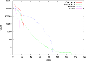
Figure 5: Edge Label Frequencies

Evaluation Metrics: (1) Average time to run queries of the same query-length, i.e., we grouped queries of same query-length, and computed average query processing time and standard deviation for those queries. Length of the query is $|label\_seq|$, e.g., an LOCR query (x, y, (*a.*a.*b.*b.*c.*d.*)) has query-length 6. Since we chose each label on randomly generated paths with uniform probability, typically an LOCR query of length 6 was generated from a randomly generated path of length 12. Observe that the query length does not indicate the length of the actual path in the graph which satisfies that query. (2) BitPath index construction time for each dataset. (3) Cumulative size of BitPath indexes for each dataset.

Since we generated the queries with random walks, for the interested reader we have given the distribution of queries by query length in Appendix-0.B.

5.3 Query Performance

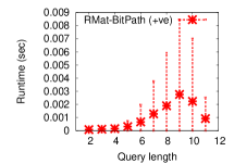
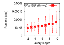
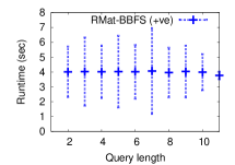
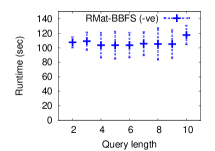
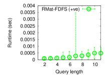
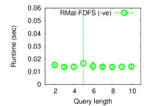
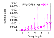
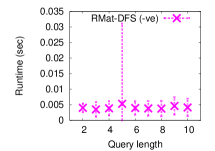
Figure 6: Mean runtime with standard deviation for varying query sizes for RMat dataset. Row 1: BitPath, Row 2: BBFS, Row 3: FDFS, Row 4: DFS

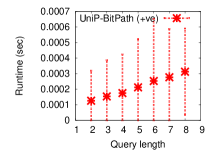
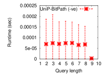
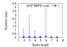
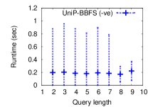
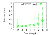
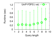
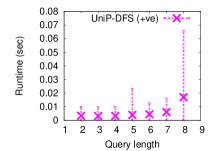
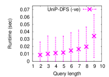
Figure 7: Mean runtime with standard deviation for varying query sizes for UniProt dataset. Row 1: BitPath, Row 2: BBFS, Row 3: FDFS, Row 4: DFS

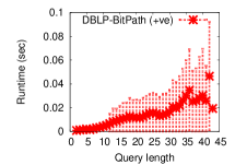
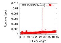
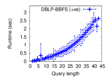
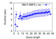
Figure 8: Mean runtime with standard deviation for varying query sizes for SwetoDBLP dataset. Row 1: BitPath, Row 2: BBFS

We ran the 50K positive and negative queries each on all four methods – BitPath, DFS, F-DFS, and B-BFS. For long running queries, we set a threshold of 15 minutes/query, i.e., if a query ran for more than 15 minutes, it is abandoned. Note the following:

– For SwetoDBLP’s positive as well as negative queries, DFS as well as F-DFS methods took significant time to finish on most queries. Hence we abandoned evaluating the queries using the two DFS methods on SwetoDBLP.

– For SwetoDBLP’s negative queries, B-BFS was taking significantly longer time to finish (more than 24 hours for 15K queries), hence we have shown results on only 15K queries.

– For R-Mat’s positive queries, B-BFS was taking long time to finish, hence after running the process for 24 hours, we abandoned further query processing and have shown results on 43K queries.

– For R-Mat’s negative queries, B-BFS was extremely slow taking more than 15 minutes for most queries, hence we have shown results only on 980 queries.

Figures 6, 7, and 8 show summarized results of Evaluation Metric (1) as outlined in the previous subsection. Each graph shows the average runtime (by the tick on the vertical line) for a group of queries with same query length along with the standard deviation for that specific group. For example, row 1 column 1 shows BitPath’s performance on R-Mat dataset for positive queries. It shows that for a group of queries of length 9, the average query runtime is 0.0003 sec and the standard deviation for this group of queries is 0.0005 sec. Note that the scale of Y-axis on each graph is different, e.g., the Y-axis for graph in row 5 column 1 for BitPath’s performance over SwetoDBLP is from 0–0.1 whereas for graph in row 5 column 2 for B-BFS’ performance on SwetoDBLP is from 0–3.

Further analysis of the results shows: B-BFS has inferior performance on the R-Mat graphs. This can be attributed to the flatter structure with not many long paths in R-Mat graphs (refer to Table 1 which shows that the “largest depth” of a node is 12), whereas SwetoDBLP graph of similar size and number of nodes has deeper structure with a lot of interleaved paths (“largest depth” of a node in SwetoDBLP is 66). The flatter structure of R-Mat favors DFS method over B-BFS while on the other hand DFS method is inferior on SwetoDBLP due to its deeper structure. Analysis of UniProt graphs shows that it contains many disconnected subgraphs, as a result of which B-BFS, F-DFS, as well as DFS fair well on this graph.

B-BFS method delivers acceptable performance on SwetoDBLP graph on positive queries. Note that this was possible due to our optimized version of B-BFS (ref. Section 5.1). The naive bidirectional BFS method was not able to deliver same performance. But as it can be noted, the performance of B-BFS method deteriorates as the length of the query increases. For negative queries, B-BFS method suffers on SwetoDBLP graph as it has to explore the entire subgraph between source and destination node. Note that on all 3 datasets with varying characteristics, BitPath delivers uniform performance on positive as well as negative queries. On average BitPath’s performance is 50 to 1000 times better for positive queries, and 1000 to 100k times better for negative queries compared to the baseline methods.

5.4 BitPath Index Size and Construction Time

The BitPath index construction time for R-Mat, UniProt, and SwetoDBLP datasets is 933 sec, 292 sec, and 809 sec respectively. Since the procedure of merging strongly connected components (SCCs) is same across all methods, the index construction time here does not include identification and merging of SCCs.

The cumulative on-disk size of N-SUCC-E, N-PRED-E, EL-ID and EID indexes for R-Mat, UniProt, and SwetoDBLP datasets are 3.7 GB, 5 GB, and 3 GB, whereas the on-disk size of these graphs is 243 MB, 394 MB, and 232 MB respectively. The uncompressed size of N-SUCC-E and N-PRED-E bit-vector indexes for R-Mat, UniProt, and SwetoDBLP graphs would have been 15,269 GB, 37,466 GB and 18,255 GB respectively (since each node has a bit-vector index of successor and predecessor edges, uncompressed size of these indexes in bytes would be #nodes $\times$ #edges $\times$ 2 / 8). Also, if N-SUCC-E and N-PRED-E indexes were stored as pure integer arrays instead of compressed bit-vectors, they would have taken 2130 GB, 738 GB, and 20 GB for R-Mat, UniProt, and SwetoDBLP graphs respectively. Note that this size is excluding the size of EL-ID and EID indexes, whereas the cumulative BitPath index sizes given above include size of all 4 indexes (N-SUCC-E, N-PRED-E, EL-ID, EID).

Thus we have shown that our approach of numbering the edges and applying run-length-encoding on the N-SUCC-E and N-PRED-E indexes (ref. Section 3) reduces the on-disk size of indexes by a factor of 7–1000 over naive indexing and storage methods.

6 Conclusion

In this paper we have addressed label-order constrained reachability queries. This problem is of specific interest for large graphs with diverse relationships (i.e., large number of edge labels in the graph). Path indexing methods for the constrained reachability or regular path queries work well on smaller graphs, but they often face scalability issues for large real life graphs. Similarly, the complexity of indexing all paths prohibits its use in practice for graphs which do not assume tree-structure.

We propose a method of building light-weight indexes on graphs using compressed bit-vectors. As shown in our evaluation, compressed bit-vectors reduce the total size of the indexes significantly. Our divide-and-conquer algorithm along with greedy-pruning strategy delivers more uniform performance across graphs of different structural characteristics. We have evaluated our method over graphs of more than 6 million nodes and 22 million edges – to the best of our knowledge, the largest among the published literature in the context of path queries on graphs. In the future, we plan to improve this method to process a wider range of path expressions and also to incorporate ways of enumerating actual path description.

Figure 9: Example XML representation of RDF graph of DBLP data

Appendix 0.A LOCR Query for XML representation of RDF

<DBLP>
<Book rdf:about="Book1">
 <chapter>
  <Chapter rdf:about="Introduction">
   <section>
    <Section rdf:about="Section1">
     <cites rdf:resource="Article2"/>
     <figure>"Example RDF graph"</figure>
    </Section>
  </section>
  </Chapter>
 </chapter>
</Book>
<Article rdf:about="Article2">
  <section>
   <Section rdf:about="Section1">
    <cites rdf:resource="Book3"/>
    <figure>"Example XML graph"</figure>
   </Section>
  </section>
</Article>
..............
<Article rdf:about="Article1000">
 <section>
  <Section rdf:about="Conclusion">
    <cites rdf:resource="Article99"/>
    <figure>"Example Path Queries"</figure>
  </Section>
 </section>
</Article>
</DBLP>

Figure 10: Example RDF graph of DBLP data

Consider texual RDF/XML representation of a DBLP dataset given in Figure 10. For simplicity we have three sample entries – “Book1”, “Article2”, and “Article1000”, although the dataset can contain several such entries, denoted by “……” in the example. The XML tree representation of this dataset with the three entries is shown in Figure 9. Note that by default RDF to XML conversion tools do not add ID/IDREFs to cross reference same URIs in the XML data. The corresponding RDF graph is shown in Figure 10. The cloud shown in the figure represents many more edges and nodes in between the citations.

Suppose the RDF graph has a transitive path with edges labeled “cites” from element “Book1” to element “Article1000”. We are interested in the following LOCR query, (Book1, Article1000, (cites)). Looking at the XML representation of the RDF graph in Figure 9, there is no such path between element “Book1” and “Article1000”, although such a path may exist between corresponding nodes in the RDF graph. This example shows that an LOCR query cannot always be translated into an equivalent path query over XML graph.

Appendix 0.B Distribution of Queries per Query Length

Figure 11 shows distribution of sampled queries according to their length. Query length is the number of edge labels appearing in the label order given in the query.

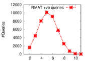
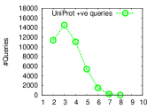
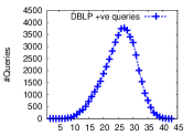
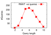
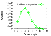
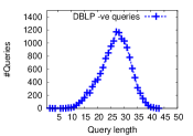
Figure 11: Distribution of queries as per query-length, Row 1: Positive queries, Row 2: Negative queries for all datasets.

References

- [1] GT-Graph. https://sdm.lbl.gov/~kamesh/software/GTgraph/.
- [2] SwetoDBLP. http://magneto.cs.uga.edu/projects/semdis/swetodblp/.
- [3] UniProt RDF. http://dev.isb-sib.ch/projects/uniprot-rdf/.
- [4] S. Abiteboul, P. Buneman, and D. Suciu. Data on the Web: From Relations to Semistructured Data and XML. Morgan Kaufmann Publishers Inc., 2000.
- [5] S. Al-Khalifa, H. V. Jagadish, et al. Structural Joins: A Primitive for Efficient XML Query Pattern Matching. In ICDE, 2002.
- [6] N. Bruno, N. Koudas, and D. Srivastava. Holistic Twig Joins: Optimal XML Pattern Matching. In SIGMOD, 2002.
- [7] D. Chakrabarti, Y. Zhan, and C. Faloutsos. R-MAT: A recursive model for graph mining. In SDM, 2004.
- [8] Q. Chen, A. Lim, and K. W. Ong. D(k)-index: an adaptive structural summary for graph-structured data. In SIGMOD, 2003.
- [9] S. Chen, H.-G. Li, J. Tatemura, W.-P. Hsiung, D. Agrawal, and K. S. Candan. Twig2Stack: bottom-up processing of generalized-tree-pattern queries over XML documents. In PVLDB, 2006.
- [10] C.-W. Chung, J.-K. Min, and K. Shim. APEX: an adaptive path index for XML data. In SIGMOD, 2002.
- [11] B. Cooper, N. Sample, et al. A Fast Index for Semistructured Data. In PVLDB, 2001.
- [12] N. El Tazi and H. V. Jagadish. BPI: XML query evaluation using bitmapped path indices. In DATAX at EDBT, 2009.
- [13] W. Fan, J. Li, et al. Adding Regular Expressions to Graph Reachability and Pattern Queries. In ICDE, 2011.
- [14] A. Gubichev and T. Neumann. Path Query Processing on Very Large RDF Graphs. In WebDB, 2011.
- [15] H. He and J. Yang. Multiresolution Indexing of XML for Frequent Queries. In ICDE, 2004.
- [16] R. Jin, H. Hong, et al. Computing Label-Constraint Reachability in Graph Databases. In SIGMOD, 2010.
- [17] R. Kaushik, P. Shenoy, P. Bohannon, and E. Gudes. Exploiting local similarity for indexing paths in graph-structured data. In ICDE, 2002.
- [18] Q. Li and B. Moon. Indexing and Querying XML Data for Regular Path Expressions. In PVLDB, 2001.
- [19] J. Lu, T. Chen, and T. W. Ling. Efficient processing of XML twig patterns with parent child edges: a look-ahead approach. In CIKM, 2004.
- [20] T. Milo and D. Suciu. Index Structures for Path Expressions. In ICDT, 1999.
- [21] M. E. J. Newman. Power laws, pareto distributions and zipf’s law. Contemporary Physics, 46(5), 2005.
- [22] S. J. van Schaik and O. de Moor. A Memory Efficient Reachability Data Structure through Bit Vector Compression. In SIGMOD, 2011.
- [23] H. Yildirim, V. Chaoji, and M. J. Zaki. GRAIL: scalable reachability index for large graphs. In PVLDB, 2010.
- [24] J. P. Yoon, V. Raghavan, and V. Chakilam. BitCube: A Three-Dimensional Bitmap Indexing for XML Documents. In SSDBM, 2001.
- [25] C. Zhang, J. Naughton, et al. On supporting containment queries in relational database management systems. In SIGMOD, 2001.