Deep phase modulation interferometry

Abstract

We have developed a method to equip homodyne interferometers with the capability to operate with constant high sensitivity over many fringes for continuous real-time tracking. The method can be considered as an extension of the “$J_{1}\dots J_{4}$” methods, and its enhancement to deliver very sensitive angular measurements through Differential Wavefront Sensing is straightforward. Beam generation requires a sinusoidal phase modulation of several radians in one interferometer arm. On a stable optical bench, we have demonstrated a long-term sensitivity over thousands of seconds of 0.1 mrad$/\sqrt{\rm Hz}$ that correspond to 20 pm$/\sqrt{\rm Hz}$ in length, and 10 nrad$/\sqrt{\rm Hz}$ in angle at millihertz frequencies.

I Introduction

Optical interferometers with sub-wavelength resolution are useful in many optical metrology applications, such as, for example, length measurements, gravitational wave detection, wavefront sensing, and surface profiling, among others. Our technique was developed in the context of continuously measuring the position and orientation of a free-floating test mass for space-based gravitational wave detection anza , although the method is useful for other applications as well. Other techniques for the optical readout of free-floating test masses at millihertz frequencies are currently under investigation, such as a polarizing heterodyne interferometer reaching a sensitivity of about $300\,\mathrm{pm}/\sqrt{\mathrm{Hz}}$ oro_berlin , a compact homodyne interferometer with a sensitivity of $100\,\mathrm{pm}/\sqrt{\mathrm{Hz}}$ oro_bmh , and a robust implementation of an optical lever with a readout noise level of $100\,\mathrm{pm}/\sqrt{\mathrm{Hz}}$ oro_napoli . Another method to do this is heterodyne interferometry as developed for LISA Pathfinder ltp with a sensitivity of better than $5\,\mathrm{pm}/\sqrt{\mathrm{Hz}}$ ltpsubtraction . The method we present here achieves an optical pathlength measurement sensitivity of the order of $20\,\mathrm{pm}/\sqrt{\mathrm{Hz}}$, and with an angular resolution better than $10\,\mathrm{nrad}/\sqrt{\mathrm{Hz}}$, both above 3 mHz. The conversion from real test mass motion to optical pathlength is given by the interferometer topology, and is in our case about a factor of 2, which yields a test mass motion resolution of approximately $10\,\mathrm{pm}/\sqrt{\mathrm{Hz}}$. Those interferometers with the highest accuracy, namely Fabry-Perot interferometers on resonance or recycled Michelson interferometers on a dark fringe geo , have a dynamic range of a small fraction of one fringe only. High resolution and wide dynamic range can be simultaneously achieved by, e.g., active feedback or heterodyning, each of which has disadvantages. Active feedback transfers the inherent non-linearity of the feedback actuator to the output signal or requires another stabilized laser and a measurement of the high-frequency beat note. Heterodyning, on the other hand, requires a complex setup to generate the two coherent beams with a constant frequency difference, typically involving two acousto-optic modulators (AOMs) with associated frequency generation and RF power amplification. Other methods to overcome these limitations involve variations of sinusoidal phase shifting interferometry sasaki_1986 ; sasaki_1987 ; deGroot_2008 ; deGroot_2009 ; Falaggis_2009 , reporting accuracies of the order of 1 nm. These methods are typically used in “single-shot” mode for static applications such as surface profiling, whereas our method is designed for continuous real-time, long-term tracking of a moving target with low noise at millihertz frequencies. In particular, the so-called “$J_{1}\dots J_{4}$” method su89 ; jin91 ; su93 , involves a sinusoidal phase modulation at a fixed frequency $f_{\rm mod}$ with modulation depths $m\approx 1\dots 5$ in one arm of the interferometer. The spectrum of the resulting photocurrent has components at integer multiples of $f_{\rm mod}$, with amplitudes that can be written in terms of the Bessel functions $J_{n}(m)$ (hence the name) and the phase difference $\varphi$ due to the optical pathlength difference. The methods then proceed to use analytical formulae to solve for the unknowns $m$ and $\varphi$, after obtaining the harmonic amplitudes from a spectrum analyzer or a Fast Fourier Transform (FFT) of the digitized time series. The accuracies reported are of order 10…100 mrad (1.7 …17 nm) for a laser wavelength of 1064 nm. We generalize this approach by using a higher modulation index $m$ (up to 10 or 20) and making use of all harmonics up to an order $N\approx m$. These are more observations than the four unknowns ($m$, $\varphi$, modulation phase and a common factor), making an analytical solution impossible. Instead we use a numerical least-squares solution which allows consistency checks and improves the signal-to-noise ratio. For our typical applications we keep $m$ near constant at an optimal value and take $\varphi$ as useful output, achieving an accuracy of better than 0.12 mrad$/\sqrt{\rm Hz}$ that correspond to 20 pm$/\sqrt{\rm Hz}$ in length, and 10 nrad$/\sqrt{\rm Hz}$ in angle at millihertz frequencies. As compared to heterodyne interferometers, more complex data processing is necessary to recover the optical pathlength from the measured photocurrent. However, with the availability of inexpensive processing power, this computational complexity is often preferable to additional optics and electronics hardware needed for the optical heterodyning.

II Theory

The signal $V_{\mathrm{PD}}(t)$ of a photodetector at the output of a phase-modulated homodyne interferometer can be expressed as

$$V_{\mathrm{PD}}(t)=A\,\left[\,1+C\,\mathrm{cos}\left(\varphi+m\,\mathrm{cos}\left(\omega_{\mathrm{m}}\,t+\psi\right)\,\right)\,\right],$$ (1)

where $\varphi$ is the interferometer phase, $m$ is the modulation depth, $\omega_{\mathrm{m}}=2\pi\,f_{\mathrm{m}}$ is the modulation frequency, $\psi$ is the modulation phase, $C\leq 1$ is the contrast, and $A$ combines nominally constant factors such as light powers and photodiode efficiencies. The interferometer output is periodic with $f_{\mathrm{m}}$ and its signal waveform characteristically depends on the interferometer phase $\varphi$. Figure 1 illustrates typical waveforms obtained for various states of $\varphi$.

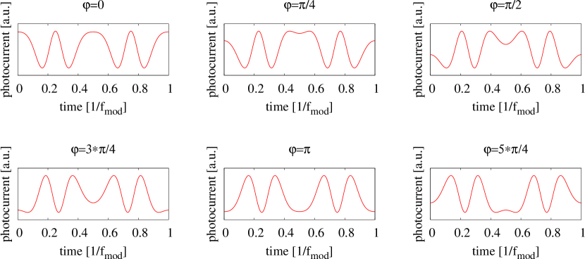
Figure 1: Waveform of the obtained interferogram for different operating points of the interferometer phase $\varphi$ with a modulation depth $m=6\,\mathrm{rad}$.

The expression of Equation 1 can be expanded into its harmonic components as:

$$V_{\rm PD}(t)=V_{\rm DC}(\varphi)+\sum\limits_{{n}=1}^{\infty}a_{n}(m,\varphi)\cos({n}(\omega_{\rm m}t+\psi))$$ (2)

with

$$a_{n}(m,\varphi) = k\,J_{n}(m)\,\cos\left(\varphi+n\frac{\pi}{2}\right),\,\,\mathrm{and}$$ (3)

$$V_{\rm DC}(\varphi) = A\left(1+C\,J_{0}(m)\cos\varphi\right),$$ (4)

where $k=2CA$, and $J_{\mathrm{n}}(m)$ are the Bessel functions. Figure 2 shows the dependence of the harmonic amplitudes $a_{n}(m,\varphi)$ in terms of $\varphi$. Our technique is centered around these harmonic amplitudes $a_{n}(m,\varphi)$ which on the one hand can be directly measured by numerical Fourier analysis of the photocurrent, and on the other hand have the above analytical relationships to the unknowns $\varphi$, $m$, $\psi$, $k$.

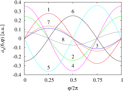
Figure 2: Dependence of the harmonics amplitudes $a_{n}(m,\varphi)$ with respect to the interferometer phase $\varphi$ with a modulation depth $m=6\,\mathrm{rad}$.

The technique we present here uses higher modulation depths $m\geq 6$ to set up an overdimensioned system of equations that can be numerically solved for the four sought parameters $\varphi$, $m$, $\psi$, and the common factor $k$ by a least-squares fit algorithm. The information of the harmonic amplitude $a_{0}(m,\varphi)$, corresponding to the DC component $V_{\rm DC}(\varphi)$ is not used by the fit algorithm, since it usually contains a higher noise level due to large variations in environmental and equipment conditions such as room illumination and electronic noise, among others. However, it is useful for computation of the interferometer visibility and alignment signals.

III Data processing

The signal $V_{\rm PD}(t)$ measured at the photodetector is digitized after appropriate analog processing and anti-alias filtering. The sampling rate $f_{\rm samp}$ is arranged to be coherent to the modulation frequency $f_{\rm mod}$. The time series is split in segments of length $N_{\mathrm{FFT}}$ samples that are processed by a Discrete Fourier Transform in order to compute $N=N_{\mathrm{FFT}}/2$ complex amplitudes $\tilde{\alpha}_{n}(m,\varphi)$. A non-linear fit algorithm is applied to match the measured $\tilde{\alpha}_{n}(m,\varphi)$ to the complex amplitudes $c_{n}$ computed from the model

$$\alpha_{n}(m,\varphi)=a_{n}(m,\varphi)\,e^{{\rm i}n\psi}.$$ (5)

There is a total of $2N$ equations that can be set up in two uncorrelated system of equations:

$$n\psi = \arctan\left(\frac{\Im\{\alpha_{n}(m,\varphi)\}}{\Re\{\alpha_{n}(m,\varphi)\}}\right),n=1,2,3\dots N,\,\,\,\,\,\,\,\,$$ (6)

$$a_{n}(m,\varphi) = \alpha_{n}(m,\varphi)\,e^{{\rm-i}n\psi},\,\,n=1,\,2,\,3\dots N,$$ (7)

where $\alpha_{n}(m,\varphi)\,e^{{\rm-i}n\psi}$ is a real number. For the measured $\tilde{\alpha}_{n}(m,\varphi)\,e^{{\rm-i}n\psi}$, this is not exactly the case due to noise and phase distortions introduced by the analog electronics. In order to solve the system of equations, a Levenberg-Marquardt fit algorithm marquardt ; numrec is applied to minimize the least-squares expression

$$\chi^{2}=\sum\limits_{n=1}^{N}{\left(\alpha_{n}(m,\varphi)-\tilde{\alpha}_{n}(m,\varphi)\right)}^{2},$$ (8)

where $\chi^{2}$ is a four dimensional function of $m$, $\varphi$, $\psi$, and $k$. In practice, these parameters barely vary between consecutive segments of length $N_{\mathrm{FFT}}$, giving good starting values for a rapid convergence of the fit. Only in the case this is not accomplished such as upon initialization or after large disturbances, a modified version of the more robust Nelder-Mead Simplex algorithm nelder is applied as initial step. In order to find best values of the modulation index $m$ and the number of bins $N$ for optimum performance, we conducted a numerical analysis of the $4\times 4$ Hessian matrix of $\chi^{2}$ that is given by

$$H=(H_{ij})=\left(\frac{\partial^{2}\chi^{2}}{\partial\Omega_{i}\partial\Omega_{j}}\right),$$ (9)

where $\Omega=\{m,\varphi,\psi,k\}$ are the four parameters. The inverse of the Hessian matrix $H^{-1}=(\eta_{ij}$) yields information about the parameter estimates on the variances $\sigma^{2}$ and correlation coefficients $\rho_{ij}$:

$$\sigma^{2}_{\Omega_{i}} \propto \eta_{ii},$$ (10)

$$\rho_{ij} = \frac{\eta_{ij}}{\sqrt{\eta_{ii}}\sqrt{\eta_{jj}}}.$$ (11)

An excursion of $\varphi$ over the range $[0,2\pi]$ –which corresponds to one interferometer fringe– was conducted in 64 steps by fixed $N$ and $m$ in order to compute the best, worst and average values of the standard deviation $\sigma_{\Omega_{i}}(N,m,\varphi)$, which are shown in Figure 3. Assuming worst case values of the variances

$$\widehat{\sigma}^{2}_{\Omega_{i}}(N,m)=\max_{\varphi\in[0,2\pi]}\sigma^{2}_{\Omega_{i}}(N,m,\varphi),$$ (12)

we run a similar analysis varying $N$ and $m$ to evaluate for best resolution of any value of $\varphi$, which is our main measurement and often not entirely under control. The results are shown in Figure 4.

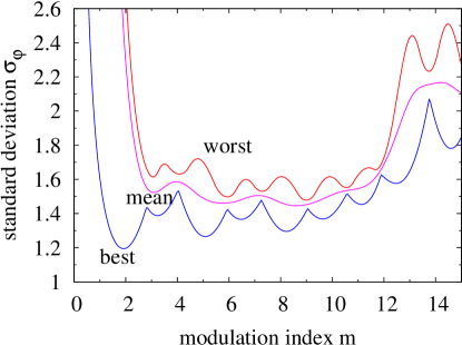
Figure 3: Ideal resolution in $\varphi$ as function of the modulation index $m$ for $N=10$, for the best and worst $\varphi$ as well as the average for all $\varphi\in[0,2\pi]$.

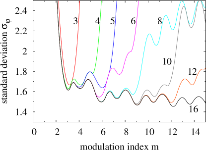
Figure 4: Ideal resolution in $\varphi$ as function of the modulation index $m$ for different orders $N$, for the worst value of $\varphi$ at each point of each curve.

This analysis revealed useful parameter estimates for $3\leq m\leq N$, and possible best values of $m$ for minimum $\sigma_{\varphi}$ in the cases of $m=6,N\geq 8$ and $m=9,N\geq 10$, suggesting best resolutions of $\varphi$. These results are only rough guidelines, since real instrument noise has not been yet considered. The dominant noise sources have, however, been investigated experimentally, as discussed in Section V below. In addition, software simulations of the fit routine were run with synthetic data as input. Hardware characteristics of the data acquisition system (DAQ) such as digitization effects and frequency response of the anti-aliasing filter were considered in the generation of mock-data, using Equation 1 as nominal noise-free model. We introduced two independent mock-data sets into two virtual DAQ channels, by linearly increasing $m$ with $N=10$ bins, and recorded the fit output (phase $\varphi$). We then computed their phase difference and extracted the nominal offset in oder to obtain the dependence of the phase fluctuations (noise) with $m$, which is shown in Figure 5.

Figure 5: Dependence of the measured phase noise with $m$.

A minimum can be observed around $m=9.5-10$, which is consistent with the analysis presented in Figure 4. Hence, a DAQ test system for real optical length measurements was set up with $N=10$ bins, and a modulation index $m\approx 9.7$.

IV Experimental setup

We have applied this technique to a very stable interferometer, namely the engineering model of the LISA Pathfinder (LPF) optical bench ltp , which consists of a 20 cm$\times$20 cm Zerodur${}^{\scriptsize{\ooalign{\hfil\raise 0.0pt\hbox{\tiny R}\hfil\crcr\text{$\mathchar 525\relax$}}}}$ baseplate with optical components fixed by hydroxide-catalysis bonding bonding . This optical bench has been extensively characterized as part of ground testing campaigns for the optical metrology of the LISA Pathfinder mission ltptests , and its optical pathlength stability has been measured to be better than 5 pm$/\sqrt{\rm Hz}$ above 1 mHz. A non-planar ring oscillator (NPRO) Nd:YAG laser producing 300 mW at 1064 nm was used as light source. For the experimental test, we chose a two-beam Mach-Zehnder interferometer, using self-assembled fiber-coupled phase modulators consisting of single-mode fiber optics coiled around ring piezo-electric transducers (RPZT) in order to reach high modulation depths (up to 10 or 20). Figure 6 shows a schematic overview of the setup.

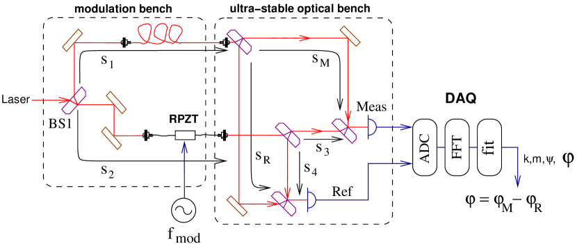
Figure 6: Schematic overview of the experiment.

The laser beam is split into two equal parts at the first beamsplitter BS1. A RPZT driven by a sinusoidal voltage of approximately 4.5 $\mathrm{V}_{\mathrm{pp}}$ at $f_{\rm mod}=280\,$Hz, produces a phase modulation of modulation depth $m\approx 9.7$ in one of the two beams. This portion of the optical setup denoted as modulation bench, contains the first beamsplitter BS1, phase modulator, and corresponding fiber coupling devices which are all mounted on a standard metal optical breadboard. A single-mode fiber feed-through is used to bring the main laser beam into a vacuum chamber where both, the modulation bench and the optical bench reside. The LISA Pathfinder optical bench is a set of four non-polarizing Mach-Zehnder interferometers, three of which have been used in these experiments. The first one –denoted M– measures distance fluctuations between two mirrors mounted on 3-axes piezo-electric actuators ltpsubtraction . A second one –denoted R– serves as phase reference to cancel common-mode pathlength fluctuations that arise at the modulation bench, such as in metal mounts, phase modulator, and fiber optics. The third interferometer –denoted F– has an intentionally large optical pathlength difference of approximately 38 cm, and is used to measure laser frequency fluctuations. If we denote by $s_{M}$ and $s_{R}$ the optical pathlengths of the measurement and reference interferometer, respectively, the phases emerging from the fit algorithm are given by

$$\varphi_{M} =\frac{2\,\pi}{\lambda}\left\{(s_{1}+s_{M})-(s_{2}+s_{3})\right\}=\frac{2\,\pi}{\lambda}\left\{(s_{M}-s_{3})+\Delta\right\},\,\,\,\,\,\,\,\,$$ (13)

$$\varphi_{R} =\frac{2\,\pi}{\lambda}\left\{(s_{1}+s_{R})-(s_{2}+s_{4})\right\}=\frac{2\,\pi}{\lambda}\left\{(s_{R}-s_{4})+\Delta\right\},\,\,\,\,\,\,\,\,$$ (14)

where $\lambda=1064$ nm is the laser wavelength, $s_{\mathrm{x}}$ are the optical paths outlined in Figure 6, and $\Delta=s_{1}-s_{2}$ represents the common-mode pathlength difference between the two beams that includes everything starting from the first beamsplitter BS1, the modulator, fiber optics up to the beamsplitters on the stable optical bench. Typically, the fluctuations of $\Delta$ are several $\mu$m on 10…1000 second time scales and thus much larger than what we want to measure. However, the optical pathlengths $s_{R}$, $s_{3}$ and $s_{4}$ are confined to the stable optical bench and have only negligible fluctuations. By measuring both $\varphi_{M}$ and $\varphi_{R}$ and computing their difference

$$\varphi=\varphi_{M}-\varphi_{R}=\frac{2\,\pi}{\lambda}\left\{s_{M}-(s_{R}+s_{3}-s_{4})\right\}$$ (15)

it is possible to cancel the common-mode fluctuations $\Delta$ and to obtain a measurement that is dominated by the fluctuations of $s_{M}$ as desired. All photodetectors are indium gallium arsenide (InGaAs) quadrant diodes with 5 mm diameter. The photocurrent of each quadrant is converted to a voltage with a low-noise transimpedance amplifier, filtered with a 9-pole 8 kHz Tschebyscheff anti-aliasing filter and digitized at a rate $f_{\mathrm{samp}}=20\,$kHz by a commercial 16-channel, 16-bit analog-to-digital converter (ADC) card installed in a standard PC running Linux. The time series are split in segments of $N_{\mathrm{FFT}}=1000$ samples and transformed by a FFT algorithm fftw . The $N=10$ complex amplitudes of bins 1…10 of $f_{\mathrm{mod}}$ at frequencies $280\dots 2800$ Hz are then fitted. This configuration allows us to reach a real-time phase measurement rate $f_{\varphi}=f_{\mathrm{samp}}/N_{\mathrm{FFT}}=20\,\mathrm{Hz}$.

V Noise investigations

During test and debugging experiments, two main noise sources were identified to limit the interferometer sensitivity with this technique, which are laser frequency noise, and the frequency response (transfer function) of the DAQ analog electronics, including photodiode transimpedance amplifiers and anti-aliasing filters. In the following we explain the coupling mechanism of these noise sources, and the mitigation strategies we implemented to counteract them.

V.1 Laser frequency noise

Laser frequency noise translates into phase readout noise in any interferometer, whose pathlength difference $\Delta s$ between the two interfering beams is not exactly zero. In the case of the LPF optical bench, this pathlength mismatch has been determined to be approximately $10\,\mathrm{mm}$ ltp . The free-running frequency noise $\delta\nu$ of an unstabilized Nd:YAG NPRO laser at $10\,\mathrm{mHz}$ has been measured to be of the order of $2\times 10^{6}\,\mathrm{Hz}/\sqrt{\mathrm{Hz}}$ ghh:2004 . The conversion factor from laser frequency fluctuations $\delta\nu$ into phase fluctuations $\delta\varphi$ is given by the difference in time of travel between the two beams $\Delta s/c$, such that an estimate of the noise level can be calculated as

$$\delta\varphi=2\pi\frac{\Delta s}{c}\delta\nu\approx 2\pi\frac{\,10^{-2}\mathrm{m}}{3\times 10^{8}\,\mathrm{m/s}}2\times 10^{6}\,\mathrm{Hz}=0.4\,\mathrm{mrad}/\sqrt{\mathrm{Hz}},$$ (16)

which limits the interferometer optical pathlength resolution $\delta s$ to

$$\delta s=\frac{\lambda}{2\pi}\,\delta\varphi=\frac{1064\,\mathrm{nm}}{2\pi}\,0.4\,\mathrm{mrad}/\sqrt{\mathrm{Hz}}=68\,\mathrm{pm}/\sqrt{\mathrm{Hz}}.$$ (17)

We implemented two mitigations strategies to correct for this effect and improve the length resolution. Both methods worked similarly well and allowed suppression of this error below the other noise terms. The first one is based on the active laser frequency stabilization, for which we have used a commercial iodine-stabilized Nd:YAG laser. The second method uses the third interferometer F (mentioned above) to independently measure a phase proportional to the amplified laser frequency fluctuations, and applies a noise subtraction technique ltpsubtraction ; felipe_phd ; noisesub that properly estimates the coupling factor and removes the contribution from the final data stream. The phase of this interferometer was read out with the same deep modulation method as the main channels, and is dominated by laser frequency fluctuations due to its large pathlength difference ($\approx 38\,$cm). A third method can also be easily implemented as an active stabilization loop by feeding back to the laser over a digital-to-analog converter the output of a digital controller that uses the difference phase extracted from interferometers F and R as error signal.

V.2 Frequency response of data acquisition system

The dominant error was identified to be the frequency response of the analog electronics of the data acquisition system, in particular the contribution of the photodiode transimpedance amplifiers and the anti-aliasing filters. The transfer function (TF) of this analog portion of the DAQ shows small ripples in its magnitude of the order of 0.9 dB. The desired parameter $\varphi$ is essentially determined by running a fit onto the relative amplitudes of the 10 measured harmonic components $\tilde{\alpha}_{n}(m,\varphi)$. The ripples are, however, large enough to alter the ratio between the harmonic amplitudes, such that the fit algorithm is disturbed, resulting in a high noise level. We removed this error by separately measuring the transfer function of each channel of the analog front end, fitting it to a model, and correcting accordingly the measured complex amplitudes $\tilde{\alpha}_{n}(m,\varphi)$ before entering the fit routine. Thus, we obtained the corresponding TF complex values $\beta_{\mathrm{n}}=b_{\mathrm{n}}\,\mathrm{e}^{i\theta_{\mathrm{n}}}$ for the 10 frequency bins of interest $280-2800$ Hz. Hence, the measured complex amplitudes $\tilde{\alpha}_{n}(m,\varphi)$ were corrected as

$$\tilde{\alpha}^{\prime}_{n}(m,\varphi)=\frac{\tilde{\alpha}_{n}(m,\varphi)}{\beta_{n}},$$ (18)

By using complex numbers, this correction also accounts for the TF phase shift, and improves the estimation capability of the modulation phase $\psi$.

VI Optical length and attitude measurements

The experimental setup of Figure 6 was used to conduct long-term interferometric length measurements on the LPF optical bench. Figure 7 shows the results obtained in form of linear spectral densities.

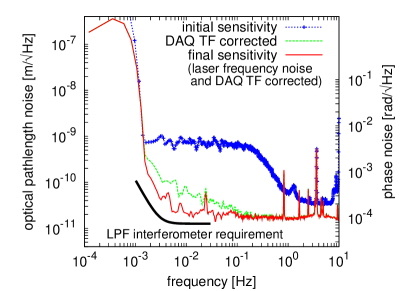
Figure 7: Sensitivity of real optical pathlength measurements. Dashed curve with crosses: initial sensitivity prior to noise correction techniques. Dashed curve: sensitivity upon correction of DAQ frequency response. Solid curve: sensitivity reach after application of noise mitigation strategies -laser frequency noise and DAQ frequency response-.

The dashed curve with crosses is the sensitivity obtained initially with this method, without applying any of the noise mitigation strategies explained in Section V. The dashed curve is the sensitivity achieved after applying the complex value correction of the DAQ frequency response to the measured harmonic amplitudes $\tilde{\alpha}_{n}(m,\varphi)$ (as given by Equation 18), resulting in a sensitivity improvement of about one order of magnitude. The solid curve is the measurement length sensitivity reached upon subtraction of laser frequency noise, which increases the length resolution in an additional factor of approximately 3.5 at 10 mHz. The measured optical pathlength sensitivity of this technique is of the order of $20\,\mathrm{pm}/\sqrt{\mathrm{Hz}}$ above 3 mHz and approximately a factor of 2 above the performance required to the LPF interferometry, which has been plotted for comparison purposes. As mentioned above, all photodetectors at the interferometer outputs on the LPF optical bench are quadrant cell diodes. The phases extracted from each individual quadrant cell are processed by a differential wavefront sensing (DWS) algorithm morrison-1 ; morrison-2 , in order to measure the interferometer alignment with high angular resolution. The results of this measurement are shown on Figure 8 as a linear spectral density.

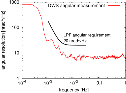
Figure 8: Angular resolution obtained by applying a DWS algorithm to the phases extracted from individual cells of a quadrant photodetector.

As it can be read from the plot, this technique reaches an angular sensitivity better than $10\,\mathrm{nrad}/\sqrt{\mathrm{Hz}}$ above 3 mHz, meeting with sufficient margin the requirements set to the LPF interferometry that have been also included in the graph as a comparison.

VII Comparison with other techniques

The only method known to the authors that allows length and angular measurements at arbitrary operating points with low noise at millihertz frequencies is heterodyne interferometry as described in Ref. ltp . The deep phase modulation method presented here needs, in comparison, much simpler beam generation hardware, namely one low-frequency phase modulator like a piezo-electric transducer, as opposed to two AOMs with RF driving electronics. On the other hand, the data processing for phase extraction is more complicated, which, however, becomes a smaller disadvantage with cheap processing power. The heterodyne method typically requires additional stabilization loops wand ; ghh-ltpnoise to reach noise levels at $\mathrm{pm}/\sqrt{\mathrm{Hz}}$, e.g. for the laser power and certain common-mode pathlengths (see Ref. ltp ). The experiments described above in Section IV show that these stabilizations are not required for the deep phase modulation technique.

VIII Conclusions

We have presented an interferometry technique for high sensitivity length and angular optical measurements. This technique is based on the deep phase modulation (over several radians) of one interferometer arm and can be considered as an extension of the well-known “$J_{1}\dots J_{4}$” method su89 ; jin91 ; su93 . The harmonic amplitudes are used to numerically solve an overdimensioned system of equations to extract the interferometer phase and other useful interferometer variables. This technique has been applied to experiments conducted on a very stable interferometer (the engineering model of the LISA Pathfinder optical bench), achieving an optical pathlength readout sensitivity of the order of $20\,\mathrm{pm}/\sqrt{\mathrm{Hz}}$ (which translates to $10\,\mathrm{pm}/\sqrt{\mathrm{Hz}}$ for free-floating test mass displacement), and alignment measurements with an angular resolution better than $10\,\mathrm{nrad}/\sqrt{\mathrm{Hz}}$ in the millihertz frequency band. This performance is comparable to the best heterodyne interferometers, and, e.g., only a factor of 2 above the LISA Pathfinder pathlength measurement requirements. Two main noise sources were identified, namely laser frequency fluctuations and the frequency response of the analog portion of the data acquisition system, which both were completely mitigated by appropriate data processing methods, hence improving the performance of this technique by over a factor 35. Unlike other interferometry techniques, no additional control loops, for instance, to actively stabilize the optical pathlength difference or laser power fluctuations, have been implemented or are required to reach the current sensitivity. Nonetheless, this could easily be done, in order to further improve the performance of this method.

References

- (1) S. Anza, M. Armano, E. Balaguer, M. Benedetti, C. Boatella, P. Bosetti, D. Bortoluzzi, N. Brandt, C. Braxmaier, M. Caldwell, L. Carbone, D. Bortoluzzi, N. Brandt, C. Braxmaier, M. Caldwell, L. Carbone, D. Bortoluzzi, N. Brandt, C. Braxmaier, M. Caldwell, L. Carbone, E. García-Berro, A.F. García Marín, R. Gerndt, A. Gianolio, D. Giardini, R. Gruenagel, A. Hammesfahr, G. Heinzel, J. Hough, D. Hoyland, M. Hueller, O. Jennrich, U. Johann, S. Kemble, C. Killow, D. Kolbe, M. Landgraf, A. Lobo, V. Lorizzo, D. Mance, K. Middleton, F. Nappo, M. Nofrarias, G. Racca, J. Ramos, D. Robertson, M. Sallusti, M. Sandford, J. Sanjuan, P. Sarra, A. Selig, D. Shaul, D. Smart, M. Smit, L. Stagnaro, T. Sumner, C. Tirabassi, S. Tobin, S. Vitale, V. Wand, H. Ward, W.J. Weber, and P. Zweifel, “The LTP experiment on the LISA Pathfinder mission,” Class. Quantum Grav. 22, S125–S138 (2005).
- (2) T. Schuldt, H.J. Kraus, D. Weise, A. Peters, U. Johann, and C. Braxmaier, “A High Sensitivity Heterodyne Interferometer as Optical Readout for the LISA Inertial Sensor,” AIP Conf. Proc. 873, 374–-378 (2006).
- (3) S.M. Aston and C.C. Speake, “An Interferometric Based Optical Read-Out Scheme For The LISA Proof-Mass,” AIP Conf. Proc. 873, 326–-333 (2006).
- (4) F. Acernese, R. De Rosa, L. Di Fiore, F. Garufi, A. La Rana, and L. Milano, “Some Progress In The Development Of An Optical Readout System For The LISA Gravitational Reference Sensor,” AIP Conf. Proc. 873, 339–-343 (2006).
- (5) G. Heinzel, C. Braxmaier, M. Caldwell, K. Danzmann, F. Draaisma, A. García, J. Hough, O. Jennrich, U. Johann, C. Killow, K. Middleton, M. te Plate, D. Robertson, A. Rüdiger, R. Schilling, F. Steier, V. Wand, and H. Ward, “Successful testing of the LISA Technology Package (LTP) interferometer engineering model,” Class. Quantum Grav. 22, S149–S154 (2005).
- (6) F. Guzmán Cervantes, F. Steier, G. Wanner, G. Heinzel, and K. Danzmann, “Subtraction of test mass angular noise in the LISA technology package interferometer,” Appl. Phys. B 90, 395–400 (2008).
- (7) S. Hild et al, “The status of GEO 600,” Class. Quantum Grav. 23, S643–S651 (2006).
- (8) O. Sasaki and H. Okazaki, ”Analysis of measurement accuracy in sinusoidal phase modulating interferometry,” Appl. Opt. 25, 3152 (1986).
- (9) O. Sasaki, H. Okazaki, and M. Sakai, ”Sinusoidal phase modulating interferometer using the integrating-bucket method,” Appl. Opt. 26, 1089 (1987)
- (10) P. de Groot and L. Deck, “New algorithms and error analysis for sinusoidal phase shifting interferometry,” Proc. of SPIE Vol. 7063, 70630K, (2008)
- (11) Peter de Groot, ”Design of error-compensating algorithms for sinusoidal phase shifting interferometry,” Appl. Opt. 48, 6788-6796 (2009)
- (12) Konstantinos Falaggis , David P Towers and Catherine E Towers, “Phase measurement through sinusoidal excitation with application to multi-wavelength Interferometry,” J. Opt. A: Pure Appl. Opt. 11 054008 (2009)
- (13) V.S. Sudarshanam and K. Srinivasan, “Linear readout of dynamic phase-change in a fiber-optic homodyne interferometer,” Opt. Lett. 14, 140–142 (1989).
- (14) W. Jin, L.M. Zhang, D. Uttamchandani, and B. Culshaw, “Modified J1 … J4 method for linear readout of dynamic phase-changes in a fiber-optic homodyne interferometer,” Appl. Opt. 30, 4496–4499 (1991).
- (15) V.S. Sudarshanam and R.O. Claus, “Generic J1…J4 method of optical-phase detection: Accuracy and range enhancement,” J. Mod. Opt. 40, 483–492 (1993).
- (16) D. Marquardt, “An Algorithm for Least-Squares Estimation of Nonlinear Parameters,” SIAM J. Appl. Math. 11, 431–441 (1963).
- (17) W.H. Press, S.A. Teukolsky, W.T. Vetterling, and B.P. Flannery, Numerical Recipes in C, The Art of Scientific Computing (Cambridge University Press, 1992).
- (18) J.A. Nelder and R. Mead, “A simplex method for function minimization,” Computer Journal 7, 308–313 (1965)
- (19) E.J. Elliffe, J. Bogenstahl, A. Deshpande, J. Hough, C. Killow, S. Reid, D. Robertson, S. Rowan, H. Ward, and G. Cagnoli, “Hydroxide-catalysis bonding for stable optical systems for space,” Class. Quantum Grav. 22, S257–S267 (2005).
- (20) A.F. García Marín et al, Albert-Einstein-Institut Hannover, Callinstr. 38, 30167 Hannover, Germany, are preparing a manuscript on “Ground testing of LISA Pathfinder optical metrology system.”
- (21) FFTW subroutine package, available from http://www.fftw.org/.
- (22) G. Heinzel, V. Wand, A. García, O. Jennrich, C. Braxmaier, D. Robertson, K. Middleton, D. Hoyland, A. Rüdiger, R. Schilling, U. Johann, and K. Danzmann, “The LTP interferometer and phasemeter,” Class. Quantum Grav. 21, S581–S587 (2004).
- (23) F. Guzmán Cervantes, “Gravitational Wave Observation from Space: optical measurement techniques for LISA and LISA Pathfinder,” Ph.D. Thesis, Leibniz Universität Hannover, Germany (2009), http://edok01.tib.uni-hannover.de/edoks/e01dh09/606793232.pdf.
- (24) F. Guzmán Cervantes, NASA Goddard Space Flight Center, 8800 Greenbelt Road, Greenbelt, MD 20771, USA, is preparing a manuscript on “Estimation and subtraction of noise contributions in the LISA Pathfinder optical metrology system.”
- (25) E. Morrison, B.J. Meers, D.I. Robertson, and H. Ward, “Experimental demonstration of an automatic alignment system for optical interferometers,” Appl. Opt. 33, 5037–5040 (1994)
- (26) E. Morrison, B.J. Meers, D.I. Robertson, and H. Ward, “Automatic alignment of optical interferometers,” Appl. Opt. 33, 5041–5049 (1994)
- (27) V. Wand, J. Bogenstahl, C. Braxmaier, K. Danzmann, A. García, F. Guzmán, G. Heinzel, J. Hough, O. Jennrich, C. Killow, D. Robertson, Z. Sodnik, F. Steier, and H. Ward, “Noise sources in the LTP heterodyne interferometer,” Class. Quantum Grav. 23, S159–S167 (2006).
- (28) G. Heinzel, V. Wand, A. García, F. Guzmán, F. Steier, C. Killow, D. Robertson, and H. Ward, “Investigation of noise sources in the LTP interferometer,” Technical note (2008), http://edoc.mpg.de/display.epl?mode=doc&id=395069&col=6&grp=1154.