Probing the inflaton: Small-scale power spectrum constraints
from measurements of the CMB energy spectrum
Abstract
In the early Universe, energy stored in small-scale density perturbations is quickly dissipated by Silk-damping, a process that inevitably generates - and -type spectral distortions of the cosmic microwave background (CMB). These spectral distortions depend on the shape and amplitude of the primordial power spectrum at wavenumbers . Here we study constraints on the primordial power spectrum derived from COBE/FIRAS and forecasted for PIXIE. We show that measurements of and impose strong bounds on the integrated small-scale power, and we demonstrate how to compute these constraints using -space window functions that account for the effects of thermalization and dissipation physics. We show that COBE/FIRAS places a robust upper limit on the amplitude of the small-scale power spectrum. This limit is about three orders of magnitude stronger than the one derived from primordial black holes in the same scale range. Furthermore, this limit could be improved by another three orders of magnitude with PIXIE, potentially opening up a new window to early Universe physics. To illustrate the power of these constraints, we consider several generic models for the small-scale power spectrum predicted by different inflation scenarios, including running-mass inflation models and inflation scenarios with episodes of particle production. PIXIE could place very tight constraints on these scenarios, potentially even ruling out running-mass inflation models if no distortion is detected. We also show that inflation models with sub-Planckian field excursion that generate detectable tensor perturbations should simultaneously produce a large CMB spectral distortion, a link that could potentially be established by PIXIE.
Subject headings:
cosmic microwave background – theory – observations – inflationPlease direct questions to ]jchluba@cita.utoronto.ca
1. Introduction
Cosmological inflation (Albrecht & Steinhardt, 1982; Guth, 1981; Linde, 1982) provides a commonly accepted explanation for both the Universe’s homogeneity and the origin of the initial curvature perturbations that seeded the growth of structure. Inflation cannot be considered a complete theory, however, until we understand the inflaton: the field that drove an epoch of accelerated expansion in the early Universe. Fortunately, the statistical properties of the initial density perturbations offer a wealth of information about inflationary physics. In single field inflation, we can in principle reconstruct the inflaton potential if the primordial power spectrum is known at all scales (e.g. Lidsey et al. 1997). However, the limited range of scales probed by the CMB and large scale structure (LSS) does not provide sufficient information to discriminate between many inflation models. Finding additional ways to measure the primordial power spectrum outside this range of scales will greatly enhance our ability to constrain the inflaton’s potential and its trajectory during inflation. In this work, we investigate how spectral distortions of the CMB caused by the dissipation of energy stored in small-scale density perturbations can provide a new probe of inflation by extending our knowledge of the primordial power spectrum from to about .
The simplest models of inflation predict a power spectrum parameterized by a nearly constant, slightly red spectral index. More complicated inflationary models can leave distinctive imprints in the primordial power spectrum. Multi-field inflation can produce primordial power spectra with steps (Silk & Turner, 1987; Polarski & Starobinsky, 1992; Adams et al., 1997) or oscillations (Achúcarro et al., 2011; Kobayashi & Takahashi, 2011; Cespedes et al., 2012). These features in the primordial power spectrum may also be generated during single-field inflation by discontinuities, kinks, and bumps in the inflaton potential (Salopek et al., 1989; Starobinskij, 1992; Ivanov et al., 1994; Starobinsky, 1998; Hunt & Sarkar, 2007; Joy et al., 2008). The primordial power spectrum may also contain information about how the inflaton interacts with other fields; for instance, particle production during inflation leaves a bump in the primordial power spectrum (Chung et al., 2000; Barnaby et al., 2009; Barnaby, 2010). Finally, several inflationary models predict enhancement of the small-scale perturbations that are generated during the later stages of inflation (Randall et al., 1996; Stewart, 1997b; Copeland et al., 1998; Covi & Lyth, 1999; Covi et al., 1999; Martin et al., 2000; Martin & Brandenberger, 2001; Ben-Dayan & Brustein, 2010; Gong & Sasaki, 2011; Lyth, 2011a; Bugaev & Klimai, 2011a).
The CMB temperature fluctuations provide a precise measurement of the primordial power spectrum on large scales, corresponding to wavenumbers (Pearson et al., 2003; Reichardt et al., 2009; Brown et al., 2009; Larson et al., 2011; Hlozek et al., 2011). Luminous red galaxies and galaxy clusters probe the matter power spectrum on similar scales (; Reid et al., 2010; Vikhlinin et al., 2009; Tinker et al., 2012; Sehgal et al., 2011), while the Lyman- forest reaches slightly smaller scales (; McDonald et al., 2006). All these observations indicate that the primordial power spectrum is nearly scale-invariant with an amplitude close to (Tegmark & Zaldarriaga, 2002; Nicholson & Contaldi, 2009; Komatsu et al., 2011; Dunkley et al., 2011; Keisler et al., 2011; Hlozek et al., 2011; Bird et al., 2011). There is no evidence of features in the primordial power spectrum on these scales (Kinney et al., 2008; Mortonson et al., 2009; Barnaby & Huang, 2009; Hamann et al., 2010; Peiris & Verde, 2010; Dvorkin & Hu, 2010; Bennett et al., 2011; Benetti et al., 2011; Dvorkin & Hu, 2011).
Our knowledge of the primordial power spectrum on smaller scales is far more limited; we only have upper bounds on its amplitude for . One of these upper bounds is derived from the limits on spectral distortions in the CMB. It was long understood that the Silk-damping (Silk, 1968) of primordial small-scale perturbations causes energy release in the early Universe (Sunyaev & Zeldovich, 1970a; Daly, 1991; Barrow & Coles, 1991; Hu et al., 1994). This gives rise to small spectral distortions of the CMB spectrum that directly depend on the shape and amplitude of the primordial power spectrum. Modes with wavenumbers dissipate their energy during the -era (redshift ), producing a non-vanishing constant residual chemical potential at high frequencies (Sunyaev & Zeldovich, 1970b; Zel’Dovich et al., 1972; Illarionov & Sunyaev, 1974; Burigana et al., 1991; Hu & Silk, 1993a), while modes with result in a -distortion. The latter is also well known in connection with the SZ-effect of clusters of galaxies (Zeldovich & Sunyaev, 1969). By accurately measuring the CMB spectrum one can therefore place robust upper limits on the possible power at small scales since the physics going into the production of these distortions is well understood.
Very precise measurements of the CMB spectrum were obtained with COBE/FIRAS (Mather et al., 1994; Fixsen et al., 1996), limiting possible deviations from a blackbody to and at 95% confidence (Fixsen et al., 1996). At lower frequencies, a similar limit on was recently obtained by ARCADE (Seiffert et al., 2011), and at is derived from TRIS (Zannoni et al., 2008; Gervasi et al., 2008). For power spectra with constant spectral index, , and normalization fixed at CMB scales, the measurements of COBE/FIRAS imply (Hu et al., 1994), but this limit is model-dependent. For instance, a small negative running, , of the spectral index weakens this bound significantly (Khatri et al., 2011; Chluba et al., 2012).
Here we generalize the COBE/FIRAS limits on spectral distortions by directly converting them into a bound on the total perturbation power at small scales. Depending on the particular inflationary model, this translates into constraints on different model parameters; the conversion can be obtained on a case-by-case basis. Also, the recently proposed CMB experiment PIXIE (Kogut et al., 2011) might be able to detect distortions that are smaller than the upper limits given by COBE/FIRAS. At this level of sensitivity, PIXIE is already close to what is required to detect the distortions arising from the dissipation of acoustic modes for a power spectrum with and no running all the way from CMB-anisotropy scales to (Chluba & Sunyaev, 2012; Khatri et al., 2011; Chluba et al., 2012). Such an improvement could rule out inflationary models with additional power at small scales, as we discuss here in more detail. Conversely, any detection of spectral distortions implies that either the power spectrum is enhanced on small scales, contrary to the predictions of the simplest inflation models, or an alternative mechanism generated CMB spectral distortions in the early Universe (e.g. particle decays).
The only other upper bounds on the amplitude of the small-scale primordial power spectrum are derived from the absence of primordial black holes (PBHs) and ultracompact minihalos (UCMHs), which are dense dark matter halos that form at high redshift (). Both PBHs and UCMHs form in regions with large primordial overdensities; an initial overdensity of is required to form a PBH (Carr, 1975; Niemeyer & Jedamzik, 1999), while UCMHs form in regions where when they enter the Hubble horizon (Ricotti & Gould, 2009; Bringmann et al., 2011). There are numerous constraints on the number density of PBHs; Josan et al. (2009) showed that these constraints imply that the amplitude of the primordial curvature power spectrum is less than 0.01-0.06 over an extremely wide range of scales (). Even though PBHs provide only a weak upper bound on the small-scale amplitude of the primordial power spectrum, they have usefully constrained inflationary models (e.g., Carr & Lidsey, 1993; Leach et al., 2000; Kohri et al., 2008; Peiris & Easther, 2008; Josan & Green, 2010a; Lyth, 2011b; Bugaev & Klimai, 2011b).
Since UCMHs form in lower density regions than those that produce PBHs, limits on their abundance can provide tighter constraints on the primordial power spectrum (Josan & Green, 2010b; Bringmann et al., 2011). Unfortunately, all current limits on the number density of UCMHs rely on the assumption that they emit gamma rays from the annihilation of dark matter particles within their high-density centers (Scott & Sivertsson, 2009; Berezinsky et al., 2010; Lacki & Beacom, 2010; Yang et al., 2011a, b, 2011; Zhang, 2011; Bringmann et al., 2011). If dark matter is a self-annihilating thermal relic, Bringmann et al. (2011) recently showed that the Large Area Telescope on the Fermi Gamma-Ray Space Telescope (Atwood et al., 2009) places the strongest constraint on the UCMH abundance; this limit implies that the amplitude of the primordial curvature power spectrum is less than to for modes with . If dark matter does not self-annihilate, then UCMHs can only be detected gravitationally. In this case, Li et al. (2012) recently showed that the Gaia satellite (Lindegren et al., 2012) will be able to detect astrometric microlensing by UCMHs and that a null detection of UCMHs by Gaia would constrain the amplitude of the primordial power spectrum to be less than for .
CMB spectral distortions probe the amplitude of the primordial power spectrum in a very different manner than PBHs and UCMHs. First of all, the physics underlying the computation of the CMB spectral distortions is very well understood, while, for example, the constraints derived from UCMHs depend on unknown properties of the dark matter particle: its mass, the abundance of its antiparticle, and its annihilation cross section. Second, since they arise from overdense regions, PBHs and UCMHs probe the high-density tail of the probability distribution function for density perturbations. The likelihood of forming a PBH or an UCMH is therefore highly sensitive to deviations from Gaussianity that enhance or suppress the abundance of high overdensities. In contrast, the CMB spectral distortion is determined by the total energy stored in density perturbations and is therefore less sensitive to the precise form of the probability distribution function. Furthermore, the expected number density of PBHs or UCMHs of a particular mass is determined by the mass variance in the sphere with radius that formed the PBH or UCMH, which is computed by convolving the primordial power spectrum with a filter function that is narrowly peaked at . Therefore, the abundance of UCMHs or PBHs of a particular mass probes the primordial power spectrum over a small range of scales. Meanwhile, the CMB spectral distortion produced by the dissipation of acoustic modes depends on the amplitude of the primordial power spectrum over a much wider range of scales (e.g., for -distortions). Consequently, limits on the power spectrum derived from CMB spectral distortions are more sensitive to the overall shape of the primordial power spectrum than those derived from the absence of UCMHs and PBHs.
Possible constraints on and for adiabatic perturbations from future measurements of and with PIXIE are discussed in detail by Chluba et al. (2012). For a power spectrum with constant spectral index, PIXIE could independently rule out at -level and a pure Harrison-Zeldovich power spectrum at -level. This limit is driven mainly by the amount of small-scale power at wavenumbers , but a simple extrapolation from CMB-anisotropy scales down to these small scales is not necessarily correct.
Here we consider more generic models for the primordial power spectrum that match the measurements from the CMB and LSS on large scales but have enhanced power on smaller scales. We begin in Section 2 by reviewing how the dissipation of small-scale inhomogeneities generates CMB spectral distortions, and we provide -space window functions that facilitate the computation of the spectral distortion generated by a given power spectrum. In Section 3, we compute the spectral distortions produced by three generic types of power spectra: power spectra with steps, kinks, and bumps. Most inflationary models that predict excess power on small scales generate power spectra with these types of features, and the constraints derived in Section 3 should be readily applicable to these models. We also specifically discuss particle production during inflation (§ 3.4), running-mass inflation (§ 3.5), and small-field inflation models ( during inflation; see § 3.6 for more details) that generate detectable gravitational waves. We summarize our analysis in Section 4.
2. Spectral distortions caused by the dissipation of acoustic modes
A consistent microphysical treatment of the dissipation of acoustic modes in the early Universe was recently given by Chluba et al. (2012). There it was shown that temperature perturbations in the photon field set up by inflation lead to an average photon energy density that in second order of the temperature fluctuations, , is slightly larger than the energy density of a blackbody at average photon temperature . The temperature anisotropies at very small scales are subsequently completely erased by shear viscosity and thermal conduction (Weinberg, 2008), processes that isotropize the photon-baryon fluid. However, the energy stored in these perturbations of the medium is not lost but merely redistributed to larger scales, causing a small increase of the average photon temperature and resulting in an average spectral distortion by the mixing of blackbody spectra with different temperatures (Zel’Dovich et al., 1972; Chluba & Sunyaev, 2004). The effective energy release depends directly on the shape of the primordial power spectrum with 1/3 of the dissipated energy sourcing -type spectral distortions that later thermalize, slowly approaching a -type distortion. The remaining 2/3 of energy just causes an adiabatic increase of the average photon temperature, without creating any distortion.
In Chluba et al. (2012) the photon Boltzmann equation for the average spectral distortion describing the effect of energy release from the dissipation of acoustic modes was derived and solved for primordial power spectra with constant spectral index and small running using the cosmological thermalization code CosmoTherm (Chluba & Sunyaev, 2012). It was shown that once the source function, , for the primordial dissipation problem is known, a rather precise description of the resulting distortion can be obtained by computing the weighted energy release in the - and -era. Given the required effective energy release rate caused by the damping of acoustic modes is determined by
| (1) |
where denotes the rate of Thomson scattering and is the Hubble expansion rate111 The approximations for and are only valid at high redshifts during the radiation-dominated era..
Defining the visibility function for spectral distortions, , with , the weighted total energy release in the - and -era is
| (2a) | ||||
| (2b) | ||||
where (cf. Hu & Silk, 1993a). At , the thermalization process is very efficient, so all the released energy just increases the specific entropy of the Universe, and hence only raises the average temperature of the CMB without causing significant spectral distortions. However, below , the CMB spectrum becomes vulnerable, and energy release leads to spectral distortions. With the simple expressions from Sunyaev & Zeldovich (1970b), and ; this can be used to estimate the expected residual distortion at high frequencies.
The energy release depends directly on the primordial power spectrum, , of curvature perturbations. Below we consider different cases for , often parametrizing it as
| (3) |
where describes the deviation of the power spectrum from the commonly used form (Kosowsky & Turner, 1995),
| (4) |
with . In the text we often refer to as standard or background power spectrum.
From observations with WMAP at large scales we have for pivot scale (Komatsu et al., 2011; Dunkley et al., 2011; Keisler et al., 2011). Without running we have from WMAP7 only, while with running the currently favored values are and (Larson et al., 2011; Komatsu et al., 2011). More recent measurements of the damping tail of the CMB power spectrum by ACT (Dunkley et al., 2011) and SPT (Keisler et al., 2011) yield222For both experiments we quote the constraint derived in combination with . and and and , respectively.
As Eq. (2) and our discussion below indicates, any constraint derived from or -type distortions to leading order is determined by computing (i) the time average energy release over the redshift interval corresponding to the and -era, and (ii) a weighted average of the total power stored over a particular range of scales. This means that the cosmological dissipation process provides a tight integral constraint on the power spectrum, which strongly limits possible inflaton trajectories in a very model-independent way. Furthermore, this constraint is not limited to just inflation scenarios but in practice should be respected by any model invoked to create the primordial seeds of structures in our Universe.
2.1. Computing the effective heating rate
Here we are mainly interested in CMB spectral distortions caused by modes that dissipate most of their energy at redshifts well before the cosmological recombination epoch (), when the Universe is still radiation-dominated and the baryon loading is negligible. In this regime one can use the tight coupling approximation to compute the required source term for the photon Boltzmann equation (Chluba et al., 2012):
where with denoting the contributions of massless neutrinos to the energy density of relativistic species; denotes conformal time and the scale factor normalized to unity today. Furthermore, is the sound horizon; is the derivative of the Thomson optical depth with respect to ; determines the damping scale with (Kaiser, 1983; Zaldarriaga & Harari, 1995)
and dimensionless sound speed of the tightly coupled photon-baryon fluid. The above expression for is based on the transfer functions for adiabatic perturbations, however, a similar formula can be obtained for isocurvature modes. Some discussion can be found in Hu & Sugiyama (1994) and Dent et al. (2012).
In the limit , the effective energy release rate for the photon field is therefore given by
| (5) |
with . For a given -mode, energy release happens when , where is about larger than the horizon scale , implying that small-scale power is dissipated well inside the horizon. During the -era, modes with contribute most to the energy release, while -distortions are mainly created by modes with .
2.2. Energy release by a single -mode
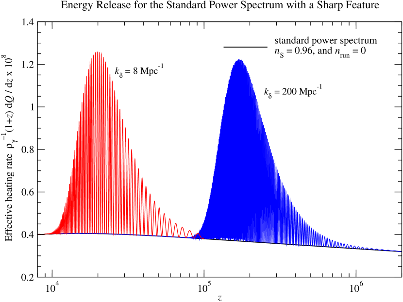
We first consider the standard power spectrum with an extremely sharp feature at some scale . In this case the modification to the power spectrum is given by , where determines the amplitude of the feature. Inserting this into Eq. (2.1) yields
| (6) |
for the associated energy release. Notice that , , and are all functions of redshift. This expression shows that power stored in a single -mode is released over a rather wide range of redshifts. The energy release peaks close to
| (7) |
but oscillates rapidly due to the sine part of the transfer function. This is illustrated in Fig. 1 for and with in both cases. For most of the energy is released during the -era, while for energy release occurs in the -era.
Since the typical variation of the energy release rate is much longer than the oscillation period, one approximately has
| (8) |
replacing , the average value over one oscillation. The effect on the CMB spectrum can now be estimated by integrating the released energy over the redshifts relevant for the -era and -era. The -era the integral can be performed analytically, while in the -era effects related to the visibility of spectral distortions have to be taken into account, i.e., see Eq. (2). With and the corresponding estimates are well approximated by
| (9a) | ||||
| (9b) | ||||
where . We mention here that the expression for is only expected to be valid for . At larger scales, baryon loading, recombination effects, and free streaming become important (Chluba et al., 2012), all of which are neglected here. These effects can be consistently treated using CosmoTherm, but for the purpose of this work, the above expression provide useful estimates for the effect on the CMB spectrum over a wide range of -values. Notice also that for the -type distortions we do not apply a sharp cutoff in redshift, but rather limit the range in -space.
2.2.1 Distortion window-function in -space
By replacing the amplitude with and integrating over , it is possible to obtain estimates for the values of and for general primordial power spectra. Since the expressions in Eq. (9) are sufficiently simple, in many cases the integral over even becomes analytic. For given small-scale power spectrum we find
| (10) |
where we set and . These expressions turn out to be very useful for estimates and simple computations, as we demonstrate below. The exponential functions act as Green’s function of the cosmological dissipation problem, and the expressions can be used for general power spectra, as long as the effect of dissipation at scales is not important. Modes in this range of wavenumbers are expected to affect the amplitude of the -distortion, which has to be computed using a full perturbation calculation (Chluba et al., 2012).
With these assumptions, Eq. (2.2.1) provides a weighted integral constraint on the small-scale power spectrum where and define window functions in -space. For a given detection of this constraint has to be satisfied by any viable inflationary model. As we see below, COBE/FIRAS already placed interesting limits on several models. Furthermore, PIXIE will improve these limits by a large margin, strongly restricting possible inflaton trajectories.
2.3. Energy release for the background power spectrum
The total energy release and spectral distortions caused by the standard power spectrum, , according to Eq. (4), were discussed in detail by Chluba et al. (2012), with simple analytic approximations given for different values of and . Here we are interested in cases with deviations from the standard shape occurring above some value of . Since the total and -distortion are given by and , to avoid double counting it is therefore useful to consider the partial energy release for the standard background power spectrum caused by modes with . For many of our examples we shall assume . In this case one has (Chluba et al., 2012)
| (11a) | ||||
| (11b) | ||||
for the total and -parameters. These expression were obtained using a detailed perturbation calculation carried out with CosmoTherm (Chluba & Sunyaev, 2012).
To compute the amount of energy release caused by modes with we start with the heating rate
| (12) |
where denotes the incomplete -function. For a scale-invariant power spectrum we can observe the redshift scaling . For this reason we usually present the effective heating rate as .
Using Eq. (2) one can easily compute the effective and -parameters caused by energy release of modes numerically. Alternatively, with Eq. (2.2.1) we find
| (13) |
where . These expressions work very well for , however, for some examples we shall use the results obtained with a full perturbation calculation to derive constraints on parameters describing possible deviations for the standard power spectrum.
3. Small-scale power spectrum constraints
In this section we discuss different small-scale power spectra, giving both the effective heating rates well before recombination, as well as possible constraints derived from and -distortions. For COBE/FIRAS the upper limits are and (Fixsen et al., 1996), while for PIXIE one expects detection limits of and (Kogut et al., 2011). When presenting results we usually assume these values, unless stated otherwise.
In the case of COBE/FIRAS this imposes a strong upper bound on the amplitude of the power spectrum, while for PIXIE the constraints should be interpreted as -detection limits. Models above this limit should lead to a signal that can be detected at more than level, implying that they can be ruled out if no distortion is found. We mention, however, that here we do not address the more difficult challenge of using the detection of a CMB spectral distortion to distinguish between different inflation scenarios. We furthermore take the optimistic point of view that foregrounds (e.g., due to synchrotron and free-free emission, dust and spinning dust) and systematics (e.g., frequency calibration, frequency-dependent beams) are sufficiently under control, so that the quoted detection limits of PIXIE can be truly achieved. More detailed forecasts including all these aspects will be required, but are beyond the scope of this paper.
3.1. Instructive upper bounds on the amplitude of the power spectrum at small scales
Let us first consider the simplest ansatz for the small-scale power spectrum: assume that it is scale-independent with amplitude over some specified range of . If we estimate the and -parameters for this case using Eq. (2.2.1), and impose the COBE/FIRAS limits, we can determine an upper bound on . Clearly, the constraints on weaken as the range of scales with enhanced power narrows.
3.1.1 Optimistic upper limit on the amplitude of the small-scale power spectrum from COBE/FIRAS
Since the power spectrum at large scales is well constrained by CMB anisotropies and LSS observations, we first assume that the small-scale power spectrum has a scale-independent amplitude [] at all scales with wavenumbers and a different constant amplitude [] for . In this case, one can derive an upper limit on from the and -limits given by COBE/FIRAS; this is an optimistic constraint on the small-scale power spectrum because we have assumed that the power spectrum is equally enhanced on all scales that contribute to and .
Carrying out the required integrals we find333We confirmed these results using CosmoTherm. and , which implies and . Using the TRIS bound, (Zannoni et al., 2008; Gervasi et al., 2008), one finds . According to the weight-functions defined in Eq. (2.2.1), the -limit is sensitive to power over , while the -limit is driven by the -range . Therefore, these constraints on are applicable to any power spectrum that has a constant amplitude over these ranges of scales. (Note that for the lower cut-off is imposed by our assumptions, rather than for physical reasons.)
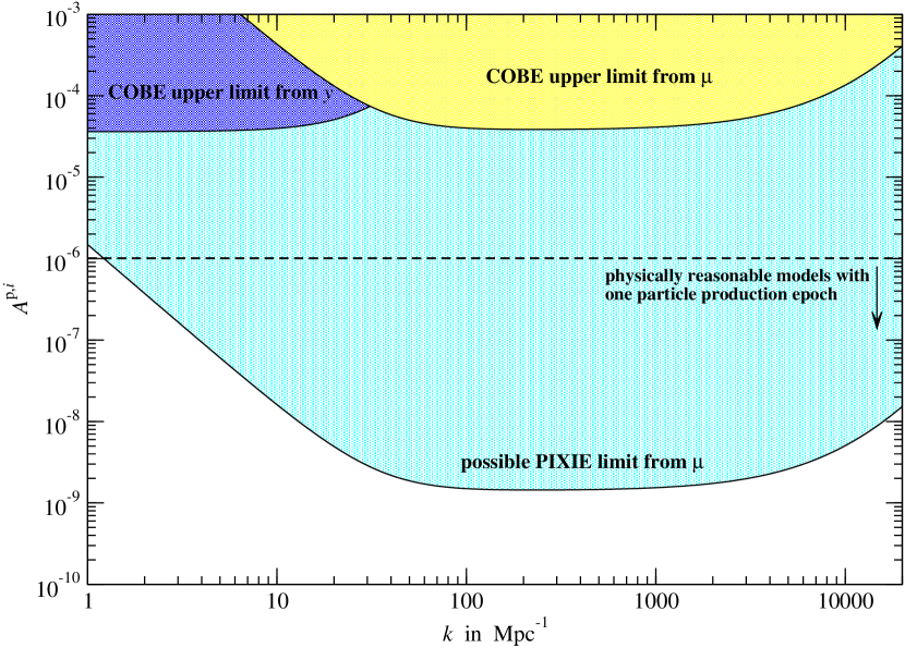
3.1.2 Comparison to constraints from PBHs and UCMHs
Another instructive example is motivated by the intention to compare the power spectrum constraints derived from CMB spectral distortions with those obtained from PBHs and UCMHs. To make this comparison, we must review how the latter are determined from observations that limit the abundance of PBHs and UCMHs. PBHs and UCMHs form in regions where the initial density contrast exceeds some critical value ( for PBHs and for UCMHs), and their masses are determined by the size of the overdense region that hosts them. If the perturbations are assumed to be Gaussian, then the probability of forming a PBH or UCMH with a certain mass depends only on the mass variance within spheres that form PBHs and UCMHs with that mass. Therefore, an upper limit on the abundance of PBHs and UCMHs with a given mass implies an upper bound on : the density variance within a sphere of radius evaluated at horizon entry in total matter gauge (Josan et al., 2009; Bringmann et al., 2011). These constraints on are then converted to constraints on the primordial curvature power spectrum at wavenumber , but this conversion assumes a specific spectral shape for .
Since only the dark matter collapses to form a UCMH, the probability of UCMH formation depends on : the dark matter mass variance. In contrast, the probability of forming a PBH depends on the total density perturbation at horizon entry, which is dominated by radiation. Since dark matter perturbations and radiation perturbations evolve differently as they enter the horizon, and have different definitions in terms of (Josan et al., 2009; Bringmann et al., 2011). Defining , then
| (14a) | ||||
| (14b) | ||||
where is a spherical Bessel function, is a filter function, and
| (15) |
where is the Euler-Mascheroni constant and Ci is the cosine integral function. When evaluating the constraints on from PBHs, Josan et al. (2009) use a Gaussian filter function, . Meanwhile, Bringmann et al. (2011) and Li et al. (2012) use the Fourier transform of a tophat window function, , when evaluating the constraints on from UCMHs. In either case, if is nearly scale-invariant, the integrals in Eqs. (14a) and (14b) are dominated by the contribution from a narrow range of values around . To derive constraints on from the upper bounds on and established by PBHs and UCMHs, it is customary to assume that is locally scale invariant, i.e. that it does not vary significantly over the limited range of scales that contribute to the mass variance at a given radius. This assumption allows us to take outside the integrals in Eqs. (14a) and (14b), making and proportional to .
Since the - and - distortions produced by the dissipation of acoustic modes receive contributions from a much wider range of scales than the mass variance does, there is no model-independent way to compare the constraints on from spectral distortions to those from PBHs and UCMHs. Any such comparison requires one to specify the scale dependence of ; we chose to make a comparison by applying the assumption of local scale invariance to the computation of CMB spectral distortions. For each scale , we assume that is nonzero only over the range of scales that contribute 99% of the integral with a Gaussian filter () and 99% of the integral with a tophat filter (). Within these scale ranges, we assume that and compute the resulting spectral distortions. Since this power spectrum gives the same mass variance (to within 1%) as a completely scale-invariant power spectrum, the constraints on the amplitude from COBE/FIRAS can now be directly compared to the constraints on the primordial power spectrum from PBHs and UCMHs; both sets of constraints make the same assumptions about the local scale-invariance of the power spectrum.
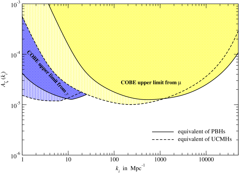
The results of our computation are summarized in Fig. 2. The typical limits for both the equivalent of the PBHs and UCMHs are for . At smaller scales the bound becomes less stringent because the thermalization process starts being very efficient. Notice also that for the shape of the constraint derived from is affected by enforcing . If we omit this restriction the curves become practically constant at a level for ; however, for these cases modification because of recombination, baryon loading and free streaming should be included to obtain accurate constraints.
For , the upper limits on from COBE/FIRAS are more than times stronger than the bound obtained from PBHs on these scales (; Josan et al., 2009). UCMHs can place stronger constraints on on these scales; if the mass of the dark matter dark matter particle is less than 5 TeV and it self-annihilates with , then the fact that Fermi-LAT has not detected gamma-ray emission from UCMHS implies that for (Bringmann et al., 2011). Even if dark matter does not self-annihilate, UCMHs could still be used to slightly improve this bound; if Gaia does not detect microlensing by UCMHs, then for for non-annihilating dark matter (Li et al., 2012). However, these constraints not only assume a particular density profile for UCMHs, but also that the UCMHs are not disrupted between their formation and today. Therefore, the bounds on from COBE/FIRAS are more robust. PIXIE could improve the bound on derived from measurement of the CMB spectrum by another two to three orders of magnitude, potentially reaching over scales .
3.2. Constraints on steps in the power spectrum
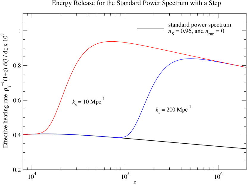
Next, we consider a step in the power spectrum at some scale , where the amplitude changes from for to for . Such a step in the primordial power spectrum could be produced by multi-stage inflation models or inflaton potentials that change slope when the inflaton reaches a certain value (Silk & Turner, 1987; Salopek et al., 1989; Starobinskij, 1992; Polarski & Starobinsky, 1992; Ivanov et al., 1994; Adams et al., 1997; Starobinsky, 1998). We will assume that the spectral index is the same on both sides of the step, and we note that the step has to fulfill the condition , as otherwise unphysical negative power is present in the power spectrum. These power spectra can be parametrized by Eq. (3) with at and otherwise. If for simplicity we assume for the background power spectrum, , we find the effective heating rate by modes with is simply given by Eq. (12) with replaced by . Similarly, the and -parameters caused by the change in power can be estimated using the expressions Eq. (2.3).
In Fig. 3 we illustrate the time-dependence of the effective energy release for and with step amplitude in both cases. The total amplitude of the power spectrum after the step therefore is . In contrast to the single-mode case, we see that the energy release no longer exhibits any oscillatory behaviour, since oscillations of several neighbouring modes cancel each other, leading to smooth energy release.
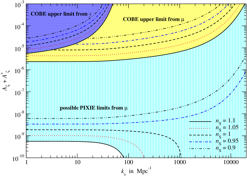
In Fig. 4 we present constraints on the total amplitude of the power spectrum after the step. We show both limits obtained from COBE/FIRAS and possible future bounds from PIXIE. In the COBE/FIRAS case the energy release from the background spectrum, , can be neglected, as it only results in for reasonable values of and (Chluba et al., 2012). The COBE limits obtained from the -distortion are most stringent in the range ; the limits get weaker at smaller scales because the thermalization process starts being very efficient. Also the -limit is stronger than the -limit because the distortion receives contributions from a slightly larger logarithmic range of wavenumbers ( for as opposed to for ).
For PIXIE we only present the possible constraint derived by measurement of . Obtaining a limit from is expected to be much harder, because at low redshifts many other astrophysical processes (e.g., energy release because of supernovae (Oh et al., 2003); shocks during large scale structure formation (Sunyaev & Zeldovich, 1972; Cen & Ostriker, 1999; Miniati et al., 2000); unresolved SZ clusters (Markevitch et al., 1991); the thermal SZ effect and second order Doppler effect from reionization (McQuinn et al., 2005)) can cause an average -distortion that is expected to be orders of magnitude larger in amplitude. For PIXIE the energy release caused by the background power spectrum no longer can be ignored, since . We therefore present the limit on just the amount of dissipation at scales , after subtracting as given by Eq. (2.3). For the shown examples with , and our results imply that respectively for , and a more than -detection of -distortions is expected even in the case for . This is simply because itself already exceeds the -detection limit of PIXIE, i.e., . Also, at about the curves become flat, indicating the point at which practically no additional -distortion is produced by modes with smaller wavenumber. In this regime only the amplitude of the -distortion is expected to change; however, unless a large distortion () is created, this signal will be hard to separate, as mentioned above. Nevertheless, simultaneous detection of (large) and could constrain the scale at which the step occurred.
Here we only considered one step, but it is easy to generalize the discussion to multiple steps. The bound will strongly depend on the distribution of and for which physical motivation should be provided, suggesting a case-by-case study is more useful. If, for example, all steps increase the total power at small scales, then the derived limits are expected to become stronger. However, for models with oscillations around a standard scale-invariant small-scale power spectrum (see, e.g., Achúcarro et al., 2011; Cespedes et al., 2012), the net effect should average out.
3.3. Constraints on a bend in the power spectrum
As a second example we consider a kink or bend in the power spectrum at some scale with the slope of the power spectrum changing from to , while remains continuous. Joy et al. (2008) showed that such changes in the spectral index result from discontinuities in the second derivative of the inflaton potential, and this model for may be used to approximate the power spectra produced by several other models that generate large perturbations on small scales (e.g., Stewart, 1997a; Ben-Dayan & Brustein, 2010; Gong & Sasaki, 2011; Lyth, 2011a; Bugaev & Klimai, 2011a; Shafi & Wickman, 2011; Hotchkiss et al., 2012). The associated power spectrum can be parametrized as
| (16) |
with . Assuming , the total power released by modes with is again given by Eq. (12) with replaced by444For Eq. (12) the pivot scale was ; to apply this expression one therefore has to rewrite , so that with at wavenumbers . . Similarly, the and -parameters caused by modes with can be estimated using the expressions Eq. (2.3).
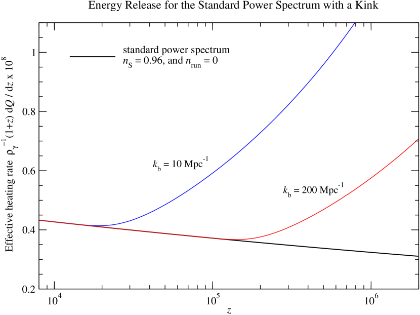
In Fig. 5 we illustrate the effective heating rate for and . One can clearly see a flaring of the energy release that starts close to according to Eq. (7). The redshift dependence suggests that the effective -parameter caused by a bend in the power spectrum is typically smaller than the -parameter. Indeed we find that for the COBE/FIRAS limits the constraints derived from are much weaker than those from , so we neglect them for the discussion below. Once again, concerns regarding confusion with low redshift -distortions are the limiting factor for constraints derived from PIXIE’s measurement of , although simultaneous detection of both and from the cosmological dissipation process would provide a deeper understanding of the shape of the small-scale power spectrum and the position of a possible kink.
We can derive constraints on the value of , and these constraints are shown in Fig. 6. The COBE/FIRAS limit on already rules out changes in the power law index by at at -level. With PIXIE this measurement will be strongly improved. For example, if the background spectrum has then even at the slope cannot change by more than without leading to an observable -distortion. Also, like in the step case, for a bend at large values of should lead to an observable signal even if the power spectrum cuts off abruptly (i.e., has a large negative value).
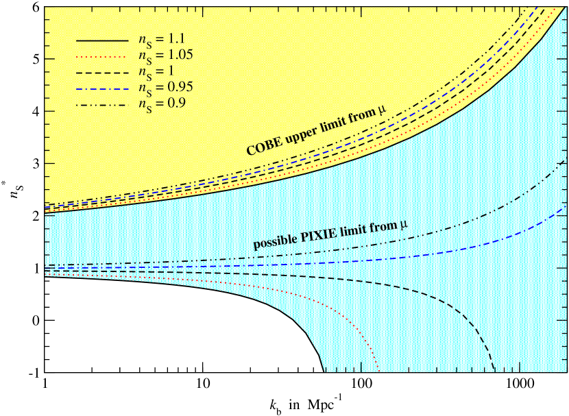
This should allow placing very tight constraints on inflationary models with flaring power spectra at small scales.
We note that PIXIE cannot constrain hybrid inflation models that use a ‘waterfall’ field to end inflation (Gong & Sasaki, 2011; Lyth, 2011a; Bugaev & Klimai, 2011a) because these models predict Mpc-1, corresponding to scales that left the horizon during the last few e-folds of inflation. Even PIXIE will be insensitive to energy release from those scales.
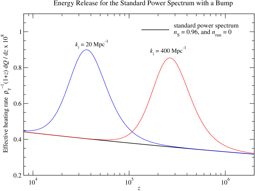
3.4. Constraints on particle production during inflation
Barnaby et al. (2009) and Barnaby (2010) showed that bursts of particle production during inflation produce localized bumps in the primordial power spectrum. Specifically, if the inflaton is coupled to another scalar field via an interaction given by , then the particles are temporarily massless when . At this time, particles are created by quantum effects, and these particles quickly become massive as moves away from . The massive particles then rescatter off the field, generating perturbations in that freeze once their wavelength exceeds the Hubble distance. The massive particles are rapidly diluted by the inflationary expansion, so only a limited range of scales receive extra perturbations.
Barnaby & Huang (2009) provided a simple parametrization for the the resulting bump in the primordial power spectrum:
| (17) |
The amplitude of the feature, , is simply related to the value of coupling constant ; . The derivation of this feature in the primordial power spectrum is only valid for (Barnaby et al., 2009), so we are primarily interested in values between and . In contrast, there are no restrictions on the location of the bump; is determined by the number of -foldings between the moment when and the end of inflation. There may also be other fields with the same coupling to the inflation, each with their own values for and . In this case, the power spectrum will contain multiple bumps, and one should sum the contributions from each episode of particle production.
Inserting Eq. 17 into Eq. (2.1), we find
| (18) |
for the effective heating rate of one feature at high redshifts (see Fig. 7 for illustration). The and -parameter caused by one feature are roughly given by
| (19a) | ||||
| (19b) | ||||
where , , and is the complementary error function. We again made use of Eq. (2.2.1) to give these simple expressions, but we also confirmed the validity of these expressions by numerically evaluating the nested integrals of the power spectrum and the heating rate.
In Fig. 8 we present the derived limits on the amplitude for one episode of particle production. The limits derived from COBE/FIRAS are weaker than the bound that is required to make the underlying calculation self-consistent. However, these bounds are still interesting, as they can be also interpreted as rather tight constraints on any other inflation models with bump-like features in the small-scale power spectrum that have a typical total width of .
The bound becomes much tighter for PIXIE, basically limiting in the range . Also, in the range , the limit derived from alone is still very interesting, although it is weaker since fewer modes related to the bump are able to release energy in the -era. Similarly, the bound becomes less stringent for because thermalization becomes efficient. Features in the small-scale power spectrum introduced by particle production are rather broad, with a significant tail of energy release towards lower redshifts, where the visibility for spectral distortions increases. Therefore, even for larger an observable -distortions is created, softening the thermalization cut-off. This implies that PIXIE could even constrain episodes of particle production with up to in an interesting way, complementing the limits obtained from CMB anisotropies and LSS at larger scales (Barnaby & Huang, 2009).
We also mention that for more than one episode of particle production, the constraints should become tighter. However, in this case again physical motivation should be given and models ought to be discussed on a case-by-case basis. Furthermore, the constraint on bumps in the power spectrum also depends on the background power spectrum at small scales. For models with direct detection of the -distortion with PIXIE could be possible even without extra bumps, so that any excess power added by particle production features should further enhance the -distortion above the detection threshold. This indicates that the interpretation of the constraint depends significantly on assumptions about the background model extrapolated from CMB and LSS scales all the way to .
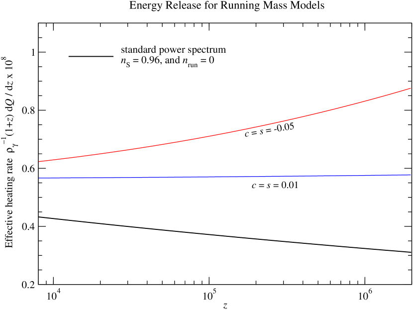
3.5. Constraining running-mass inflation models
For our next explicit example, we consider running-mass inflation, which is a single-field supersymmetric inflation model that can generate enhanced power on small scales (Stewart, 1997a, b; Covi & Lyth, 1999; Covi et al., 1999). These models assume that the dominant loop correction to the inflaton potential is , where is the renormalization scale. In this case, the renormalization-group-improved inflaton potential is , implying that the mass of the inflaton effectively changes during inflation. Consequently, running-mass models offer a solution to the -problem of supergravity inflation; in supergravity, scalar fields usually have masses that are too large to drive inflation, but in running-mass inflation, can be large when is equal to the reduced Planck mass while being small enough to permit inflation at smaller values of .
To ensure that the inflaton potential is sufficiently flat, inflation must occur near an extremum of the inflaton potential. Therefore, we can approximate the inflaton mass as
where is the value of at the extremum of and evaluated at . The -parameter may be positive or negative, but explicit formulations of running-mass inflation in the context of supersymmetry have (e.g. Covi et al., 2004). Given this linear approximation for , the primordial power spectrum can be parametrized as (cf. Covi & Lyth, 1999; Covi et al., 2004)
| (20) |
In this expression , and , where is the value of the inflaton when the mode with wavenumber exited the Hubble horizon, e-folds before the end of inflation. Note that can be positive or negative, depending on the sign of and the direction rolls during inflation. It follows that , where is the inflaton value at the end of inflation. Therefore, values of with imply that , which requires certain fine-tuning.
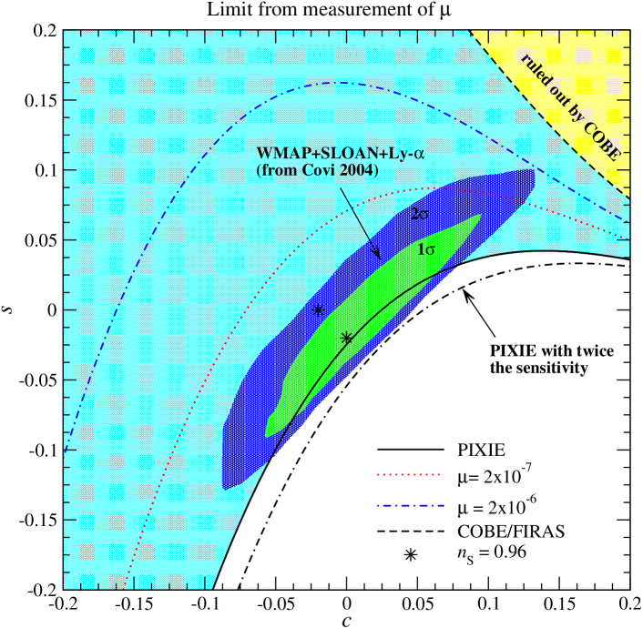
One can also directly relate and to the usual spectral index and running (Covi et al., 2004):
| (21a) | ||||
| (21b) | ||||
Observational parameter limits on and derived using previous WMAP (Bennett et al., 2003), SDSS (Tegmark et al., 2004) and Ly- forest (Seljak et al., 2005) measurements are shown as closed contours in Fig. 10 (Covi et al., 2004), limiting the range of allowed models to cases with and . According to Eq. (21), the allowed models typically have positive running with and . This indicates that updated constraints from the latest CMB and LSS measurements that favor negative running might already further narrow down the allowed parameter space in comparison to Covi et al. (2004). However, the two running-mass models that match the current best-fit WMAP7 model without running, at are still viable (cf. Fig. 10).
Using Eq. (20) we can easily compute the effective heating rate and distortion parameters for different values of and . In Fig. 9 we illustrate this for two running-mass models that are in agreement with the constraints of Covi et al. (2004). The departure from the standard background spectrum occurs very gradually, so that in comparison with the standard power spectrum, both enhanced and -distortions are expected in nearly all cases.
To compute the limits on the parameters and shown in Fig. 10, we use the expressions given by Eq. (2.2.1). We also confirmed that a more precise computation practically gives the same result. The COBE/FIRAS limit on does rule out a significant part of the theoretically allowed parameter space, however, in comparison to the constraints given by Covi et al. (2004) no improvement is achieved. On the other hand, PIXIE might rule out many running-mass inflation models at the level, narrowing the possible parameter space down to a slim region around and . Furthermore, PIXIE with twice the sensitivity could rule out running-mass inflation models if no distortion is detected. We also computed the limit from measurement of the -parameter, but found that the constraint was always much weaker.
3.6. Spectral distortions for small-field models generating detectable gravitational waves
Another interesting class of inflation models that predicts an enhancement of the power spectrum at small scales is a class of small-field models that generate a detectable gravitational wave (GW) signal (Ben-Dayan & Brustein, 2010; Shafi & Wickman, 2011; Hotchkiss et al., 2012). Within this class, models with larger GW signal are also expected to produce excess power at small scales. Therefore, the detection of both a GW signal and a CMB spectral distortion at the predicted level would provide strong evidence for these models.
The exact power spectrum has to be evaluated numerically (as done in Ben-Dayan & Brustein, 2010) and exhibits a richer phenomenology than the standard nearly scale-invariant case, even when is included. The ability to produce a detectable GW signal with limited field excursion, , is based on the fact that the slow-roll parameter is non-monotonic from the time the CMB scales left the horizon until inflation ends. More explicitly, is initially large enough to produce a detectable GW signal, then it decreases to a smaller value for most of the duration of inflation. At a later time, increases to unity and inflation ends. The scales of exit the horizon while is decreasing; since , small-scale power is enhanced. The power spectrum also exhibits a maximum at a smaller scale that exits the horizon just before begins to increase.
Since here we are only interested in the possible CMB distortions we do not repeat the exact numerical calculation, but use the ‘improved power spectrum’ form (Eq. (78) of Lyth & Riotto, 1999), which captures all essential features of the model. A more complete likelihood analysis is deferred to later work. We calculated the and distortions for some models discussed in Ben-Dayan & Brustein (2010), however, we added specific models555Following the definitions of Ben-Dayan & Brustein (2010), these correspond to: and ; , and . with small tensor to scalar ratio . The GW signal of these scenarios could potentially be detected with PIXIE.
As mentioned above, we find that the level of and distortions is linked to the GW signal. This is because a larger GW signal requires a larger change in between CMB scales and smaller scales. We therefore expect a bigger enhancement of small-scale perturbations. For one of the models with relatively large GW signal, , we obtain and . At this level, we expect a definite detection by PIXIE.
However, the distortions decrease with , so that for the spectral distortions reduce to the level similar to the standard power spectrum without running, i.e., and (Chluba et al., 2012).
Therefore, we have an interesting cross-check between GW detection and CMB distortions. In the optimistic case, if the model of inflation realized in nature is of this type, then we expect PIXIE to detect both tensor perturbations and CMB distortions.
4. Discussion and conclusion
We considered constraints on the small-scale power spectrum derived from present and future measurements of the spectral distortions in the CMB. We introduced -space window functions for - and -distortions that account for the effect of thermalization and dissipation physics and facilitate computing the effective - and -parameters directly from the primordial power spectrum at (see Eq. (2.2.1) in § 2.2). This defines an integral constraint that places tight limits on the shape of the small-scale power spectrum and, by extension, constrains possible inflation scenarios or any other model of the early Universe that is invoked to create the primordial seeds of the structures we see today.
We discussed different generic cases for the small-scale power spectrum, demonstrating how this integral constraint can be translated into limits on power spectrum parameters. In particular, we derived limits from the COBE/FIRAS bounds on and , showing that for these upper limits on the amplitude of the power spectrum are roughly times stronger than those derived from PBHs at similar scales (see § 3.1.2). Limits obtained with UCMHs supersede the COBE/FIRAS limits by more than an order of magnitude, but these limits depend on the properties of the dark matter particle. In contrast, the constraints from CMB distortions can be obtained in a very model-independent way, relying on well-understood physics related to the thermalization and dissipation of acoustic modes. We also showed that PIXIE will improve the bounds derived from and by about three orders of magnitude. PIXIE could therefore open a new window to the early Universe, extending the lever arm from CMB-anisotropy and LSS scales all the way to .
As explicit examples, we studied the constraints on inflation models with episodes of particle production (§ 3.4) and running inflaton mass (§ 3.5). We demonstrated that PIXIE could complement the upper limits on particle production derived at CMB and LSS scales, extending them from up to (see Fig. 8). We also showed that PIXIE might have the opportunity to rule out running-mass inflation models if no spectral distortion at the level of is found (see Fig. 10 and § 3.5). Similarly, for other models with flaring small-scale power spectrum (e.g. Barnaby et al., 2011) our computations indicate that strong bounds could be placed on the viable parameter space. As argued in § 3.6, small-field inflation models ( during inflation) with significant GW signal should simultaneously produce large CMB spectral distortions, an intriguing connection that could potentially be established by PIXIE.
The possible limits derived from future PIXIE measurements of suffer from confusion with -type distortions created at low redshifts because significant differences between these two signal are not expected. However, one effect might help in this respect: as shown by Chluba & Sunyaev (2009) energy release before recombination causes uncompensated cycles of atomic transitions in helium and hydrogen. This leads to extra emission and absorption features in the cosmological recombination radiation (Chluba & Sunyaev, 2006; Sunyaev & Chluba, 2009). At both high and very low frequencies, the associated effect is larger or comparable to the -distortion itself, so that a delicate interplay between the thermalization process and the recombination radiation is expected. This effect might distinguish -type distortions imprinted before the end of recombination from those coming from low redshifts, if precise spectral measurements are performed (Chluba & Sunyaev, 2009). In particular, distortions at high frequencies, created by the Lyman-series of hydrogen and doubly ionized helium, as well as the series of neutral helium might be very interesting in this respect. However, to give a definite answer a more detailed computation is required, simultaneously including the effect of atomic transitions in the thermalization calculation.
The derived bounds are obtained under the assumption that the only process causing energy release at high redshifts is the dissipation of acoustic modes. However, other forms of energy release are possible. For example, as recently shown by Chluba & Sunyaev (2012) and Khatri et al. (2011), the adiabatic cooling of ordinary matter inevitably leads to small negative - and -type distortions with amplitude and . This process is based on well understood physics, and hence the associated distortion can be predicted with high precision. Nevertheless, many other possible sources of energy release exist including annihilating or decaying particles (e.g., see Burigana et al., 1991; Hu & Silk, 1993a, b; McDonald et al., 2001); evaporating black holes (see Carr et al., 2010, and references therein); superconducting strings (Ostriker & Thompson, 1987; Tashiro et al., 2012); or dissipation of magnetic fields (Jedamzik et al., 2000). (See Chluba & Sunyaev (2012) for detailed computations of the associated distortions with CosmoTherm.)
All these processes come with significant uncertainties, so it is unclear at which level distortions can be expected. Therefore, the constraints obtained here should be considered as the most conservative upper limits, since any additional energy release not caused by the dissipation of acoustic modes will only tighten the bounds on the primordial power spectrum. An interpretation of a detection of CMB spectral distortion therefore requires more careful consideration of the differences (e.g., the mixture between and ; the detailed shape of the distortion at low frequencies) in the distortions for each case, which in principle can be accurately computed using CosmoTherm. In addition, differences in the spatial distribution, although expected to be tiny for primordial distortions (Chluba et al., 2012), might help distinguish different scenarios in the future. Correlations of the distortion with CMB anisotropies could furthermore reveal non-Gaussianity of the power spectrum (Pajer & Zaldarriaga, 2012).
We close by mentioning that even if the parameters describing the power spectrum at CMB-anisotropy and LSS scales fully determine the small-scale power spectrum, a measurement of and could be interpreted as an independent confirmation of these values.
Moreover, it is important to note that the determination of and with CMB measurements is subject to uncertainties in recombination dynamics (Shaw & Chluba, 2011). While standard recombination physics seems to be under control (e.g., see Dubrovich & Grachev, 2005; Kholupenko et al., 2007; Switzer & Hirata, 2008; Wong et al., 2008; Fendt et al., 2009; Rubiño-Martín et al., 2010; Grin & Hirata, 2010; Chluba & Thomas, 2011; Ali-Haïmoud & Hirata, 2011), possible surprises due to neglected standard or non-standard processes could still await us. Directly constraining the recombination dynamics from CMB anisotropy measurements itself is challenging (Farhang et al., 2011), so some theoretical uncertainty in the values of and is unavoidable.
Therefore, a detection of -distortions at the level extrapolated from CMB and LSS scale constraints would be very reassuring, further demonstrating the great potential of this new window to the early Universe.
Acknowledgements. The authors are grateful to Neil Barnaby and Eric Switzer for discussions and comments on the manuscript. Research at CITA is supported by NSERC. ALE and IBD are also supported by the Perimeter Institute for Theoretical Physics and the Canadian Institute for Advanced Research. Research at the Perimeter Institute is supported by the Government of Canada through Industry Canada and by the Province of Ontario through the Ministry of Research and Innovation. The authors also acknowledge the use of the GPC supercomputer at the SciNet HPC Consortium. SciNet is funded by: the Canada Foundation for Innovation under the auspices of Compute Canada; the Government of Ontario; Ontario Research Fund - Research Excellence; and the University of Toronto.
References
- Achúcarro et al. (2011) Achúcarro, A., Gong, J.-O., Hardeman, S., Palma, G. A., & Patil, S. P. 2011, JCAP, 1, 30
- Adams et al. (1997) Adams, J. A., Ross, G. G., & Sarkar, S. 1997, Nuclear Physics B, 503, 405
- Albrecht & Steinhardt (1982) Albrecht, A. J., & Steinhardt, P. J. 1982, Phys.Rev.Lett, 48, 1220
- Ali-Haïmoud & Hirata (2011) Ali-Haïmoud, Y., & Hirata, C. M. 2011, Phys.Rev.D, 83, 043513
- Atwood et al. (2009) Atwood et al. 2009, ApJ, 697, 1071
- Barnaby (2010) Barnaby, N. 2010, Phys.Rev.D, 82, 106009
- Barnaby & Huang (2009) Barnaby, N., & Huang, Z. 2009, Phys.Rev.D, 80, 126018
- Barnaby et al. (2009) Barnaby, N., Huang, Z., Kofman, L., & Pogosyan, D. 2009, Phys.Rev.D, 80, 043501
- Barnaby et al. (2011) Barnaby, N., Pajer, E., & Peloso, M. 2011, ArXiv:1110.3327
- Barrow & Coles (1991) Barrow, J. D., & Coles, P. 1991, MNRAS, 248, 52
- Ben-Dayan & Brustein (2010) Ben-Dayan, I., & Brustein, R. 2010, JCAP, 9, 7
- Benetti et al. (2011) Benetti, M., Lattanzi, M., Calabrese, E., & Melchiorri, A. 2011, Phys.Rev., D84, 063509
- Bennett et al. (2011) Bennett, C., Hill, R., Hinshaw, G., Larson, D., Smith, K., et al. 2011, Astrophys.J.Suppl., 192, 17
- Bennett et al. (2003) Bennett, C. L., et al. 2003, ApJS, 148, 1
- Berezinsky et al. (2010) Berezinsky, V., Dokuchaev, V., Eroshenko, Y., Kachelrieß, M., & Solberg, M. A. 2010, Phys.Rev.D, 81, 103529
- Bird et al. (2011) Bird, S., Peiris, H. V., Viel, M., & Verde, L. 2011, MNRAS, 413, 1717
- Bringmann et al. (2011) Bringmann, T., Scott, P., & Akrami, Y. 2011, ArXiv:1110.2484v1
- Brown et al. (2009) Brown, M. L., et al. 2009, ApJ, 705, 978
- Bugaev & Klimai (2011a) Bugaev, E., & Klimai, P. 2011a, JCAP, 11, 28
- Bugaev & Klimai (2011b) —. 2011b, ArXiv:1112.5601
- Burigana et al. (1991) Burigana, C., Danese, L., & de Zotti, G. 1991, A&A, 246, 49
- Carr (1975) Carr, B. J. 1975, ApJ, 201, 1
- Carr et al. (2010) Carr, B. J., Kohri, K., Sendouda, Y., & Yokoyama, J. 2010, Phys.Rev.D, 81, 104019
- Carr & Lidsey (1993) Carr, B. J., & Lidsey, J. E. 1993, Phys.Rev.D, 48, 543
- Cen & Ostriker (1999) Cen, R., & Ostriker, J. P. 1999, ApJ, 514, 1
- Cespedes et al. (2012) Cespedes, S., Atal, V., & Palma, G. A. 2012, ArXiv:1201.4848
- Chluba et al. (2012) Chluba, J., Khatri, R., & Sunyaev, R. A. 2012, ArXiv:1202.0057
- Chluba & Sunyaev (2004) Chluba, J., & Sunyaev, R. A. 2004, A&A, 424, 389
- Chluba & Sunyaev (2006) —. 2006, A&A, 458, L29
- Chluba & Sunyaev (2009) —. 2009, A&A, 501, 29
- Chluba & Sunyaev (2012) —. 2012, MNRAS, 419, 1294
- Chluba & Thomas (2011) Chluba, J., & Thomas, R. M. 2011, MNRAS, 412, 748
- Chung et al. (2000) Chung, D. J. H., Kolb, E. W., Riotto, A., & Tkachev, I. I. 2000, Phys.Rev.D, 62, 043508
- Copeland et al. (1998) Copeland, E. J., Liddle, A. R., Lidsey, J. E., & Wands, D. 1998, Phys.Rev.D, 58, 063508
- Covi & Lyth (1999) Covi, L., & Lyth, D. H. 1999, Phys.Rev.D, 59, 063515
- Covi et al. (2004) Covi, L., Lyth, D. H., Melchiorri, A., & Odman, C. J. 2004, Phys.Rev.D, 70, 123521
- Covi et al. (1999) Covi, L., Lyth, D. H., & Roszkowski, L. 1999, Phys.Rev.D, 60, 023509
- Daly (1991) Daly, R. A. 1991, ApJ, 371, 14
- Dent et al. (2012) Dent, J. B., Easson, D. A., & Tashiro, H. 2012, ArXiv:1202.6066
- Dubrovich & Grachev (2005) Dubrovich, V. K., & Grachev, S. I. 2005, Astronomy Letters, 31, 359
- Dunkley et al. (2011) Dunkley, J., et al. 2011, ApJ, 739, 52
- Dvorkin & Hu (2010) Dvorkin, C., & Hu, W. 2010, Phys.Rev.D, 82, 043513
- Dvorkin & Hu (2011) —. 2011, Phys.Rev.D, 84, 063515
- Farhang et al. (2011) Farhang, M., Bond, J. R., & Chluba, J. 2011, ArXiv:1110.4608
- Fendt et al. (2009) Fendt, W. A., Chluba, J., Rubiño-Martín, J. A., & Wandelt, B. D. 2009, ApJS, 181, 627
- Fixsen et al. (1996) Fixsen, D. J., Cheng, E. S., Gales, J. M., Mather, J. C., Shafer, R. A., & Wright, E. L. 1996, ApJ, 473, 576
- Gervasi et al. (2008) Gervasi, M., Zannoni, M., Tartari, A., Boella, G., & Sironi, G. 2008, ApJ, 688, 24
- Gong & Sasaki (2011) Gong, J.-O., & Sasaki, M. 2011, JCAP, 3, 28
- Grin & Hirata (2010) Grin, D., & Hirata, C. M. 2010, Phys.Rev.D, 81, 083005
- Guth (1981) Guth, A. H. 1981, Phys.Rev.D, 23, 347
- Hamann et al. (2010) Hamann, J., Shafieloo, A., & Souradeep, T. 2010, JCAP, 1004, 010
- Hlozek et al. (2011) Hlozek, R., et al. 2011, ArXiv:1105.4887
- Hotchkiss et al. (2012) Hotchkiss, S., Mazumdar, A., & Nadathur, S. 2012, JCAP, 2, 8
- Hu et al. (1994) Hu, W., Scott, D., & Silk, J. 1994, ApJL, 430, L5
- Hu & Silk (1993a) Hu, W., & Silk, J. 1993a, Phys.Rev.D, 48, 485
- Hu & Silk (1993b) —. 1993b, Physical Review Letters, 70, 2661
- Hu & Sugiyama (1994) Hu, W., & Sugiyama, N. 1994, ApJ, 436, 456
- Hunt & Sarkar (2007) Hunt, P., & Sarkar, S. 2007, Phys.Rev., D76, 123504
- Illarionov & Sunyaev (1974) Illarionov, A. F., & Sunyaev, R. A. 1974, Astronomicheskii Zhurnal, 51, 1162
- Ivanov et al. (1994) Ivanov, P., Naselsky, P., & Novikov, I. 1994, Phys.Rev.D, 50, 7173
- Jedamzik et al. (2000) Jedamzik, K., Katalinić, V., & Olinto, A. V. 2000, Physical Review Letters, 85, 700
- Josan & Green (2010a) Josan, A. S., & Green, A. M. 2010a, Phys.Rev.D, 82, 047303
- Josan & Green (2010b) —. 2010b, Phys.Rev.D, 82, 083527
- Josan et al. (2009) Josan, A. S., Green, A. M., & Malik, K. A. 2009, Phys.Rev.D, 79, 103520
- Joy et al. (2008) Joy, M., Sahni, V., & Starobinsky, A. A. 2008, Phys.Rev.D, 77, 023514
- Kaiser (1983) Kaiser, N. 1983, MNRAS, 202, 1169
- Keisler et al. (2011) Keisler, R., et al. 2011, ApJ, 743, 28
- Khatri et al. (2011) Khatri, R., Sunyaev, R. A., & Chluba, J. 2011, arXiv:1110.0475
- Kholupenko et al. (2007) Kholupenko, E. E., Ivanchik, A. V., & Varshalovich, D. A. 2007, MNRAS, 378, L39
- Kinney et al. (2008) Kinney, W. H., Kolb, E. W., Melchiorri, A., & Riotto, A. 2008, Phys.Rev., D78, 087302
- Kobayashi & Takahashi (2011) Kobayashi, T., & Takahashi, F. 2011, JCAP, 1, 26
- Kogut et al. (2011) Kogut, A., et al. 2011, JCAP, 7, 25
- Kohri et al. (2008) Kohri, K., Lyth, D. H., & Melchiorri, A. 2008, JCAP, 4, 38
- Komatsu et al. (2011) Komatsu, E., et al. 2011, ApJS, 192, 18
- Kosowsky & Turner (1995) Kosowsky, A., & Turner, M. S. 1995, Phys.Rev.D, 52, 1739
- Lacki & Beacom (2010) Lacki, B. C., & Beacom, J. F. 2010, ApJL, 720, L67
- Larson et al. (2011) Larson, D., et al. 2011, ApJS, 192, 16
- Leach et al. (2000) Leach, S. M., Grivell, I. J., & Liddle, A. R. 2000, Phys.Rev.D, 62, 043516
- Li et al. (2012) Li, F., Erickcek, A. L., & Law, N. M. 2012, ArXiv:1202.1284
- Lidsey et al. (1997) Lidsey, J. E., Liddle, A. R., Kolb, E. W., Copeland, E. J., Barreiro, T., & Abney, M. 1997, Reviews of Modern Physics, 69, 373
- Linde (1982) Linde, A. D. 1982, Phys. Lett. B, 108, 389
- Lindegren et al. (2012) Lindegren, L., Lammers, U., Hobbs, D., O’Mullane, W., Bastian, U., & Hernández, J. 2012, A&A in press
- Lyth (2011a) Lyth, D. H. 2011a, JCAP, 7, 35
- Lyth (2011b) —. 2011b, ArXiv:1107.1681
- Lyth & Riotto (1999) Lyth, D. H. D. H., & Riotto, A. A. 1999, Phys. Rep., 314, 1
- Markevitch et al. (1991) Markevitch, M., Blumenthal, G. R., Forman, W., Jones, C., & Sunyaev, R. A. 1991, ApJL, 378, L33
- Martin & Brandenberger (2001) Martin, J., & Brandenberger, R. H. 2001, Phys.Rev.D, 63, 123501
- Martin et al. (2000) Martin, J., Riazuelo, A., & Sakellariadou, M. 2000, Phys.Rev.D, 61, 083518
- Mather et al. (1994) Mather, J. C., et al. 1994, ApJ, 420, 439
- McDonald et al. (2001) McDonald, P., Scherrer, R. J., & Walker, T. P. 2001, Phys.Rev.D, 63, 023001
- McDonald et al. (2006) McDonald, P., et al. 2006, ApJS, 163, 80
- McQuinn et al. (2005) McQuinn, M., Furlanetto, S. R., Hernquist, L., Zahn, O., & Zaldarriaga, M. 2005, ApJ, 630, 643
- Miniati et al. (2000) Miniati, F., Ryu, D., Kang, H., Jones, T. W., Cen, R., & Ostriker, J. P. 2000, ApJ, 542, 608
- Mortonson et al. (2009) Mortonson, M. J., Dvorkin, C., Peiris, H. V., & Hu, W. 2009, Phys.Rev., D79, 103519
- Nicholson & Contaldi (2009) Nicholson, G., & Contaldi, C. R. 2009, JCAP, 7, 11
- Niemeyer & Jedamzik (1999) Niemeyer, J. C., & Jedamzik, K. 1999, Phys.Rev.D, 59, 124013
- Oh et al. (2003) Oh, S. P., Cooray, A., & Kamionkowski, M. 2003, MNRAS, 342, L20
- Ostriker & Thompson (1987) Ostriker, J. P., & Thompson, C. 1987, ApJL, 323, L97
- Pajer & Zaldarriaga (2012) Pajer, E., & Zaldarriaga, M. 2012, ArXiv:1201.5375
- Pearson et al. (2003) Pearson, T. J., et al. 2003, ApJ, 591, 556
- Peiris & Easther (2008) Peiris, H. V., & Easther, R. 2008, JCAP, 7, 24
- Peiris & Verde (2010) Peiris, H. V., & Verde, L. 2010, Phys.Rev., D81, 021302
- Polarski & Starobinsky (1992) Polarski, D., & Starobinsky, A. A. 1992, Nucl. Phys., B385, 623
- Randall et al. (1996) Randall, L., SoljačiĆ, M., & Guth, A. H. 1996, Nuclear Physics B, 472, 377
- Reichardt et al. (2009) Reichardt, C. L., et al. 2009, ApJ, 694, 1200
- Reid et al. (2010) Reid, B. A., et al. 2010, MNRAS, 404, 60
- Ricotti & Gould (2009) Ricotti, M., & Gould, A. 2009, ApJ, 707, 979
- Rubiño-Martín et al. (2010) Rubiño-Martín, J. A., Chluba, J., Fendt, W. A., & Wandelt, B. D. 2010, MNRAS, 403, 439
- Salopek et al. (1989) Salopek, D. S., Bond, J. R., & Bardeen, J. M. 1989, Phys.Rev.D, 40, 1753
- Scott & Sivertsson (2009) Scott, P., & Sivertsson, S. 2009, Physical Review Letters, 103, 211301
- Sehgal et al. (2011) Sehgal, N., et al. 2011, ApJ, 732, 44
- Seiffert et al. (2011) Seiffert, M., et al. 2011, ApJ, 734, 6
- Seljak et al. (2005) Seljak, U., et al. 2005, Phys.Rev.D, 71, 103515
- Shafi & Wickman (2011) Shafi, Q., & Wickman, J. R. 2011, Physics Letters B, 696, 438
- Shaw & Chluba (2011) Shaw, J. R., & Chluba, J. 2011, MNRAS, 415, 1343
- Silk (1968) Silk, J. 1968, ApJ, 151, 459
- Silk & Turner (1987) Silk, J., & Turner, M. S. 1987, Phys.Rev.D, 35, 419
- Starobinskij (1992) Starobinskij, A. A. 1992, Soviet Journal of Experimental and Theoretical Physics Letters, 55, 489
- Starobinsky (1998) Starobinsky, A. A. 1998, Gravitation and Cosmology, 4, 88
- Stewart (1997a) Stewart, E. D. 1997a, Physics Letters B, 391, 34
- Stewart (1997b) —. 1997b, Phys.Rev.D, 56, 2019
- Sunyaev & Chluba (2009) Sunyaev, R. A., & Chluba, J. 2009, Astronomische Nachrichten, 330, 657
- Sunyaev & Zeldovich (1970a) Sunyaev, R. A., & Zeldovich, Y. B. 1970a, ApSS, 9, 368
- Sunyaev & Zeldovich (1970b) —. 1970b, ApSS, 7, 20
- Sunyaev & Zeldovich (1972) —. 1972, A&A, 20, 189
- Switzer & Hirata (2008) Switzer, E. R., & Hirata, C. M. 2008, Phys.Rev.D, 77, 083008
- Tashiro et al. (2012) Tashiro, H., Sabancilar, E., & Vachaspati, T. 2012, ArXiv:1202.2474
- Tegmark & Zaldarriaga (2002) Tegmark, M., & Zaldarriaga, M. 2002, Phys.Rev.D, 66, 103508
- Tegmark et al. (2004) Tegmark, M., et al. 2004, Phys.Rev.D, 69, 103501
- Tinker et al. (2012) Tinker, J. L., et al. 2012, ApJ, 745, 16
- Vikhlinin et al. (2009) Vikhlinin, A., et al. 2009, ApJ, 692, 1060
- Weinberg (2008) Weinberg, S. 2008, Cosmology (Oxford University Press)
- Wong et al. (2008) Wong, W. Y., Moss, A., & Scott, D. 2008, MNRAS, 386, 1023
- Yang et al. (2011) Yang, Y., Chen, X., Lu, T., & Zong, H. 2011, Eur. Phys. J. Plus, 126, 123
- Yang et al. (2011a) Yang, Y., Feng, L., Huang, X., Chen, X., Lu, T., & Zong, H. 2011a, JCAP, 12, 20
- Yang et al. (2011b) Yang, Y., Huang, X., Chen, X., & Zong, H. 2011b, Phys.Rev.D, 84, 043506
- Zaldarriaga & Harari (1995) Zaldarriaga, M., & Harari, D. D. 1995, Phys.Rev.D, 52, 3276
- Zannoni et al. (2008) Zannoni, M., Tartari, A., Gervasi, M., Boella, G., Sironi, G., De Lucia, A., Passerini, A., & Cavaliere, F. 2008, ApJ, 688, 12
- Zel’Dovich et al. (1972) Zel’Dovich, Y. B., Illarionov, A. F., & Syunyaev, R. A. 1972, Soviet Journal of Experimental and Theoretical Physics, 35, 643
- Zeldovich & Sunyaev (1969) Zeldovich, Y. B., & Sunyaev, R. A. 1969, ApSS, 4, 301
- Zhang (2011) Zhang, D. 2011, MNRAS, 418, 1850