FDB: A Query Engine for Factorised Relational Databases

Abstract

Factorised databases are relational databases that use compact factorised representations at the physical layer to reduce data redundancy and boost query performance.

This paper introduces FDB, an in-memory query engine for select-project-join queries on factorised databases. Key components of FDB are novel algorithms for query optimisation and evaluation that exploit the succinctness brought by data factorisation. Experiments show that for data sets with many-to-many relationships FDB can outperform relational engines by orders of magnitude.

1 Introduction

This paper introduces FDB, an in-memory query engine for select-project-join queries on factorised relational data.

At the outset of this work lies the observation that relations can admit compact, factorised representations that can effectively boost the performance of relational processing. The relationship between relations and their factorised representations is on a par with the relationship between logic functions in disjunctive normal form and their equivalent nested forms obtained by algebraic factorisation.

Example 1.

Consider a database of a grocery retailer containing delivery orders, stock availability at different locations, availability of dispatcher units for the individual locations, and grocery producers with items they produce and locations they supply to (Figure 1). A query $Q_{1}$ that finds all orders with their respective items, possible locations to retrieve them from, and dispatchers available to deliver them, returns the following result (shown only partially):

$Q_{1}=\textrm{Order}\Join_{\textrm{item}}\textrm{Store}\Join_{\textrm{location}}\textrm{Disp}$
oid	item	location	dispatcher
01	Milk	Istanbul	Adnan
01	Milk	Istanbul	Yasemin
01	Milk	Izmir	Adnan
01	Milk	Antalya	Volkan
$\dots$

This query result can be expressed as a relational expression built using singleton relations, union, and product, whereby each singleton relation ${\langle{\color[rgb]{0,0,1}\mathrm{v}}\rangle}$ holds one value v, each tuple is a product of singleton relations, and an arbitrary relation is a union of products of singleton relations:

$${\langle{\color[rgb]{0,0,1}\mathrm{01}}\rangle}\times{\langle{\color[rgb]{0,0,1}\mathrm{Milk}}\rangle}\times{\langle{\color[rgb]{0,0,1}\mathrm{Istanbul}}\rangle}\times{\langle{\color[rgb]{0,0,1}\mathrm{Adnan}}\rangle}\cup$$

$${\langle{\color[rgb]{0,0,1}\mathrm{01}}\rangle}\times{\langle{\color[rgb]{0,0,1}\mathrm{Milk}}\rangle}\times{\langle{\color[rgb]{0,0,1}\mathrm{Istanbul}}\rangle}\times{\langle{\color[rgb]{0,0,1}\mathrm{Yasemin}}\rangle}\cup$$

$${\langle{\color[rgb]{0,0,1}\mathrm{01}}\rangle}\times{\langle{\color[rgb]{0,0,1}\mathrm{Milk}}\rangle}\times{\langle{\color[rgb]{0,0,1}\mathrm{Izmir}}\rangle}\times{\langle{\color[rgb]{0,0,1}\mathrm{Adnan}}\rangle}\cup$$

$${\langle{\color[rgb]{0,0,1}\mathrm{01}}\rangle}\times{\langle{\color[rgb]{0,0,1}\mathrm{Milk}}\rangle}\times{\langle{\color[rgb]{0,0,1}\mathrm{Antalya}}\rangle}\times{\langle{\color[rgb]{0,0,1}\mathrm{Volkan}}\rangle}\cup\ldots$$

A more compact equivalent representation can be obtained by algebraic factorisation using distributivity of product over union and commutativity of product and union:

$${\langle{\color[rgb]{0,0,1}\mathrm{Milk}}\rangle}\times{\langle{\color[rgb]{0,0,1}\mathrm{01}}\rangle}\times({\langle{\color[rgb]{0,0,1}\mathrm{Istanbul}}\rangle}\times({\langle{\color[rgb]{0,0,1}\mathrm{Adnan}}\rangle}\cup{\langle{\color[rgb]{0,0,1}\mathrm{Yasemin}}\rangle})\cup$$

$$\phantom{{\langle{\color[rgb]{0,0,1}\mathrm{Milk}}\rangle}\times{\langle{\color[rgb]{0,0,1}\mathrm{01}}\rangle}\times(}{\langle{\color[rgb]{0,0,1}\mathrm{Izmir}}\rangle}\times{\langle{\color[rgb]{0,0,1}\mathrm{Adnan}}\rangle}\cup{\langle{\color[rgb]{0,0,1}\mathrm{Antalya}}\rangle}\times{\langle{\color[rgb]{0,0,1}\mathrm{Volkan}}\rangle})\cup$$

$${\langle{\color[rgb]{0,0,1}\mathrm{Cheese}}\rangle}\times({\langle{\color[rgb]{0,0,1}\mathrm{01}}\rangle}\cup{\langle{\color[rgb]{0,0,1}\mathrm{03}}\rangle})\times({\langle{\color[rgb]{0,0,1}\mathrm{Istanbul}}\rangle}\times({\langle{\color[rgb]{0,0,1}\mathrm{Adnan}}\rangle}\cup{\langle{\color[rgb]{0,0,1}\mathrm{Yasemin}}\rangle})\cup$$

$$\phantom{{\langle{\color[rgb]{0,0,1}\mathrm{Cheese}}\rangle}\times({\langle{\color[rgb]{0,0,1}\mathrm{01}}\rangle}\cup{\langle{\color[rgb]{0,0,1}\mathrm{03}}\rangle})\times(}{\langle{\color[rgb]{0,0,1}\mathrm{Antalya}}\rangle}\times{\langle{\color[rgb]{0,0,1}\mathrm{Volkan}}\rangle})\cup$$

$${\langle{\color[rgb]{0,0,1}\mathrm{Melon}}\rangle}\times({\langle{\color[rgb]{0,0,1}\mathrm{02}}\rangle}\cup{\langle{\color[rgb]{0,0,1}\mathrm{03}}\rangle})\times{\langle{\color[rgb]{0,0,1}\mathrm{Istanbul}}\rangle}\times({\langle{\color[rgb]{0,0,1}\mathrm{Adnan}}\rangle}\cup{\langle{\color[rgb]{0,0,1}\mathrm{Yasemin}}\rangle})$$

This factorised representation has the following structure: for each item, we construct a union of its possible orders and a union of its possible locations with dispatchers. This nesting structure together with the attribute names form the schema of the factorised representation, which we call a factorisation tree, or f-tree for short.

Figure 2 depicts several f-trees; the leftmost one ($\mathcal{T}_{1}$) captures the nesting structure of the above factorisation. The second f-tree ($\mathcal{T}_{2}$) is an alternative nesting structure for the same query result, where for each location, we construct a union of its items and orders and a union of dispatchers:

$${\langle{\color[rgb]{0,0,1}\mathrm{Istanbul}}\rangle}\times({\langle{\color[rgb]{0,0,1}\mathrm{Milk}}\rangle}\times{\langle{\color[rgb]{0,0,1}\mathrm{01}}\rangle}\cup{\langle{\color[rgb]{0,0,1}\mathrm{Cheese}}\rangle}\times({\langle{\color[rgb]{0,0,1}\mathrm{01}}\rangle}\cup{\langle{\color[rgb]{0,0,1}\mathrm{03}}\rangle})\cup$$

$$\phantom{{\langle{\color[rgb]{0,0,1}\mathrm{Istanbul}}\rangle}\times(}{\langle{\color[rgb]{0,0,1}\mathrm{Melon}}\rangle}\times({\langle{\color[rgb]{0,0,1}\mathrm{02}}\rangle}\cup{\langle{\color[rgb]{0,0,1}\mathrm{03}}\rangle}))\times({\langle{\color[rgb]{0,0,1}\mathrm{Adnan}}\rangle}\cup{\langle{\color[rgb]{0,0,1}\mathrm{Yasemin}}\rangle})\cup$$

$${\langle{\color[rgb]{0,0,1}\mathrm{Izmir}}\rangle}\times{\langle{\color[rgb]{0,0,1}\mathrm{Milk}}\rangle}\times{\langle{\color[rgb]{0,0,1}\mathrm{01}}\rangle}\times{\langle{\color[rgb]{0,0,1}\mathrm{Adnan}}\rangle}\cup$$

$${\langle{\color[rgb]{0,0,1}\mathrm{Antalya}}\rangle}\times({\langle{\color[rgb]{0,0,1}\mathrm{Milk}}\rangle}\times{\langle{\color[rgb]{0,0,1}\mathrm{01}}\rangle}\cup{\langle{\color[rgb]{0,0,1}\mathrm{Cheese}}\rangle}\times({\langle{\color[rgb]{0,0,1}\mathrm{01}}\rangle}\cup{\langle{\color[rgb]{0,0,1}\mathrm{03}}\rangle}))\times{\langle{\color[rgb]{0,0,1}\mathrm{Volkan}}\rangle}$$

The factorised result of the query $Q_{2}=\textrm{Produce}\Join_{\textrm{supplier}}\textrm{Serve}$ over the f-tree $\mathcal{T}_{3}$ given in Figure 2 is:

$${\langle{\color[rgb]{0,0,1}\mathrm{Guney}}\rangle}\times({\langle{\color[rgb]{0,0,1}\mathrm{Milk}}\rangle}\cup{\langle{\color[rgb]{0,0,1}\mathrm{Cheese}}\rangle})\times{\langle{\color[rgb]{0,0,1}\mathrm{Antalya}}\rangle}\cup$$

$${\langle{\color[rgb]{0,0,1}\mathrm{Dikici}}\rangle}\times{\langle{\color[rgb]{0,0,1}\mathrm{Milk}}\rangle}\times({\langle{\color[rgb]{0,0,1}\mathrm{Istanbul}}\rangle}\cup{\langle{\color[rgb]{0,0,1}\mathrm{Izmir}}\rangle}\cup{\langle{\color[rgb]{0,0,1}\mathrm{Antalya}}\rangle})\cup$$

$${\langle{\color[rgb]{0,0,1}\mathrm{Byzantium}}\rangle}\times{\langle{\color[rgb]{0,0,1}\mathrm{Melon}}\rangle}\times{\langle{\color[rgb]{0,0,1}\mathrm{Istanbul}}\rangle}\hskip 56.00012pt\Box$$

Orders
oid	item
01	Milk
01	Cheese
02	Melon
03	Cheese
03	Melon

(a)

Store
location	item
Istanbul	Milk
Istanbul	Cheese
Istanbul	Melon
Izmir	Milk
Antalya	Milk
Antalya	Cheese

(b)

Disp
dispatcher	location
Adnan	Istanbul
Adnan	Izmir
Yasemin	Istanbul
Volkan	Antalya

(c)

Produce
supplier	item
Guney	Milk
Guney	Cheese
Dikici	Milk
Byzantium	Melon

(d)

Serve
supplier	location
Guney	Antalya
Dikici	Istanbul
Dikici	Izmir
Dikici	Antalya
Byzantium	Istanbul

(e)

Figure 1: An example database for a grocery retailer.

$$\psset{levelsep=7mm,nodesep=1.0pt,treesep=5mm}\pstree{\TR{\textrm{item}}}{\TR{\textrm{oid}}\pstree{\TR{\textrm{location}}}{\TR{\textrm{dispatcher}}}}\hskip 22.50003pt\psset{levelsep=7mm,nodesep=1.0pt,treesep=5mm}\pstree{\TR{\textrm{location}}}{\pstree{\TR{\textrm{item}}}{\TR{\textrm{oid}}}\TR{\textrm{dispatcher}}}\hskip 22.50003pt\psset{levelsep=7mm,nodesep=1.0pt,treesep=5mm}\pstree{\TR{\textrm{supplier}}}{\TR{\textrm{item}}\TR{\textrm{location}}}\hskip 22.50003pt\psset{levelsep=7mm,nodesep=1.0pt,treesep=5mm}\pstree{\TR{\textrm{item}}}{\pstree{\TR{\textrm{supplier}}}{\TR{\textrm{location}}}}\hskip 22.50003pt\psset{levelsep=7mm,nodesep=1.0pt,treesep=5mm}\pstree{\TR{\textrm{item}}}{\TR{\textrm{oid}}\pstree{\TR{\textrm{location}}}{\TR{\textrm{dispatcher}}}\pstree{\TR{\textrm{supplier}}}{\TR{\textrm{location}}}}\hskip 22.50003pt\psset{levelsep=7mm,nodesep=1.0pt,treesep=5mm}\pstree{\TR{\textrm{item}}}{\TR{\textrm{oid}}\pstree{\TR{\textrm{location}}}{\TR{\textrm{dispatcher}}\TR{\textrm{supplier}}}}$$

Figure 2: Factorisation trees used in Example 1. From left to right: $\mathcal{T}_{1}$ and $\mathcal{T}_{2}$ for the result of query $Q_{1}$; $\mathcal{T}_{3}$ and $\mathcal{T}_{4}$ for the result of $Q_{2}$; $\mathcal{T}_{5}$ is obtained after joining $\mathcal{T}_{1}$ and $\mathcal{T}_{4}$ on item, and $\mathcal{T}_{6}$ is $\mathcal{T}_{5}$ after joining on location.

Factorisations are ubiquitous. They are arguably most known for minimisation of Boolean functions [8] but can be useful in a number of read-optimised database scenarios. The scenario we consider in this paper is that of factorising large intermediate and final results to speed-up query evaluation on data sets with many-to-many relationships. A further scenario we envisage is that of compiled databases: these are static databases, such as databases encoding the human genome [15], that can be aggressively factorised to efficiently support a particular scientific workload. In provenance and probabilistic databases, factorisations of provenance polynomials [11] are used for compact encoding of large provenance (the GeneOntology database has records with 10MB provenance) [18] and for efficient query evaluation [16, 22]. Factorisations are a natural fit whenever we deal with a large space of possibilities or choices. For instance, data models for design specifications, such as the AND/OR trees [14], are based on incompleteness and non-determinism and are captured by factorised representations. Formalisms for incomplete information, such as world-set decompositions [4, 17], rely on factorisations of universal relations encoding very large sets of possible worlds; they are products of unions of products of tuples. Outside data management scenarios, factorised relations can be used to compactly represent the space of feasible solutions to configuration problems in constraint satisfaction, where we need to connect a fixed finite set of given components so as to meet a given objective while respecting given constraints [5].

Factorised representations have several key properties that make them appealing in the above mentioned scenarios.

They can be exponentially more succinct than the relations they encode. For instance, a product of $n$ relations needs size exponential in $n$ for a relational result, but only linear in the size of the input relations for a factorised result. Recent work has established tight bounds on the size of factorised query results [19]: For any select-project-join query $Q$, there is a rational number $s(Q)$ such that for any database $\mathbf{D}$, there exists a factorised representation $E$ of $Q(\mathbf{D})$ with size $O(|\mathbf{D}|^{s(Q)})$, and within the class of representations whose structures are given by factorisation trees, there is no factorisation of smaller size. The parameter $s(Q)$ is the fractional edge cover number of a particular subquery of $Q$, and there are arbitrarily large queries $Q$ for which $s(Q)=1$. Moreover, the exponential gap between the sizes of $E$ and of $Q(\mathbf{D})$ also holds between the times needed to compute $E$ and $Q(\mathbf{D})$ directly from the input database $\mathbf{D}$.

Further succinctness can be achieved using dictionary-based compression and null suppression of data values [20]. Compressing entire vertical partitions of relations as done in c-store [9] is not compatible with our factorisation approach since it breaks the relational structure.

Notwithstanding succinctness, factorised representations of query results allow for fast (constant-delay) enumeration of tuples. More succinct representations are definitely possible, e.g., binary join decompositions [10] or just the pair of the query and the database [6], but then retrieving any tuple in the query result is already NP-hard. Factorised representations can thus be seen as compilations of query results that allow for efficient subsequent processing.

By construction, factorised representations reduce redundancy in the data and boost query performance using a mixture of vertical (product) and horizontal (union) data partitioning. This goal is shared with a large body of work on normal forms [2] and columnar stores [7] that considers join (or general vertical) decompositions, and with partitioning-based automated physical database design [3, 13]. In the latter case, the focus is on partitioning input data such that the performance of a particular workload is maximised.

Finally, factorised representations are relational algebra expressions with well-understood semantics. Their relational nature sets them apart from XML documents, object-oriented databases, and nested objects [2], where the goal is to avoid the rigidity of the relational model. Moreover, in our setting, a query result can admit several equivalent factorised representations and the goal is to find one of small size. The Verso project [1] points out compactness and modelling benefits of non-first-normal-form relations and considers hierarchical data representations that are special cases of factorised representations. It does not focus on factorisations and thus neither on the search for ones of small sizes.

A factorised database presents relations at the logical layer but uses succinct factorised representations at the physical layer. The FDB query engine can thus not only compute factorised query results for input relational databases, but can evaluate queries directly on input factorised databases.

Example 2.

Consider now the query $Q_{1}\Join_{\textrm{location,item}}Q_{2}$ on factorised representations: Find possible suppliers of ordered items. Joining the above factorisations over the f-trees $\mathcal{T}_{1}$ and $\mathcal{T}_{3}$ on the attributes location and item is not immediate, since tuples with equal values for location and item appear scattered in the factorisation over $\mathcal{T}_{3}$. If we restructure the factorisation of $Q_{2}$’s result to follow the f-tree $\mathcal{T}_{4}$ so that tuples are grouped by item first, we obtain

$${\langle{\color[rgb]{0,0,1}\mathrm{Milk}}\rangle}\times({\langle{\color[rgb]{0,0,1}\mathrm{Guney}}\rangle}\times{\langle{\color[rgb]{0,0,1}\mathrm{Antalya}}\rangle}\cup$$

$$\phantom{{\langle{\color[rgb]{0,0,1}\mathrm{Milk}}\rangle}\times(}{\langle{\color[rgb]{0,0,1}\mathrm{Dikici}}\rangle}\times({\langle{\color[rgb]{0,0,1}\mathrm{Istanbul}}\rangle}\cup{\langle{\color[rgb]{0,0,1}\mathrm{Izmir}}\rangle}\cup{\langle{\color[rgb]{0,0,1}\mathrm{Antalya}}\rangle}))$$

$${\langle{\color[rgb]{0,0,1}\mathrm{Cheese}}\rangle}\times{\langle{\color[rgb]{0,0,1}\mathrm{Guney}}\rangle}\times{\langle{\color[rgb]{0,0,1}\mathrm{Antalya}}\rangle}\cup$$

$${\langle{\color[rgb]{0,0,1}\mathrm{Melon}}\rangle}\times{\langle{\color[rgb]{0,0,1}\mathrm{Byzantium}}\rangle}\times{\langle{\color[rgb]{0,0,1}\mathrm{Istanbul}}\rangle},$$

which can be readily joined with the factorisation over $\mathcal{T}_{1}$ on the attribute item, since both factorisations have items as topmost values. The factorisation of the join on item follows the f-tree $\mathcal{T}_{5}$, where we simply merged the roots of the two f-trees. An excerpt of this factorisation is

$${\langle{\color[rgb]{0,0,1}\mathrm{Milk}}\rangle}\times{\langle{\color[rgb]{0,0,1}\mathrm{01}}\rangle}\times({\langle{\color[rgb]{0,0,1}\mathrm{Istanbul}}\rangle}\times({\langle{\color[rgb]{0,0,1}\mathrm{Adnan}}\rangle}\cup{\langle{\color[rgb]{0,0,1}\mathrm{Yasemin}}\rangle})\cup$$

$$\phantom{{\langle{\color[rgb]{0,0,1}\mathrm{Milk}}\rangle}\times{\langle{\color[rgb]{0,0,1}\mathrm{01}}\rangle}\times(}{\langle{\color[rgb]{0,0,1}\mathrm{Izmir}}\rangle}\times{\langle{\color[rgb]{0,0,1}\mathrm{Adnan}}\rangle}\cup{\langle{\color[rgb]{0,0,1}\mathrm{Antalya}}\rangle}\times{\langle{\color[rgb]{0,0,1}\mathrm{Volkan}}\rangle})$$

$$\phantom{{\langle{\color[rgb]{0,0,1}\mathrm{Milk}}\rangle}}\times({\langle{\color[rgb]{0,0,1}\mathrm{Guney}}\rangle}\times{\langle{\color[rgb]{0,0,1}\mathrm{Antalya}}\rangle}\cup$$

$$\phantom{{\langle{\color[rgb]{0,0,1}\mathrm{Milk}}\rangle}\times(}{\langle{\color[rgb]{0,0,1}\mathrm{Dikici}}\rangle}\times({\langle{\color[rgb]{0,0,1}\mathrm{Istanbul}}\rangle}\cup{\langle{\color[rgb]{0,0,1}\mathrm{Izmir}}\rangle}\cup{\langle{\color[rgb]{0,0,1}\mathrm{Antalya}}\rangle}))\cup\dots,$$

To perform the second join condition on location, we first need for each item to rearrange the subexpression for suppliers and locations, so that it is grouped by locations as opposed to suppliers. This amounts to swapping supplier and location in $\mathcal{T}_{5}$. The join on location can now be performed between the possible locations of each item. The obtained factorisation follows the schema $\mathcal{T}_{6}$ in Figure 2. $\Box$

Examples 1 and 2 highlight challenges involved in computing factorised representations of query results.

Firstly, a query result may have different (albeit equivalent) factorised representations whose sizes can differ by an exponential factor. We seek f-trees that define succinct representations of query results for all input (relational or factorised) databases. Such f-trees can be statically derived from the query and the input schema, but are independent of the database content. Query optimisation thus has to consider two objectives: minimising the cost of computing a factorised query result from the (possibly factorised) input database, and minimising the size of this output representation. In addition to the standard query operators selection, projection, and product, the search space for a good query and factorisation plan, or f-plan for short, needs to consider specific operators for restructuring schemas and factorisations. We propose two such operators: a swap operator, which exchanges a given child with its parent in an f-tree, and a push-up operator, which moves an entire sub-tree up in the f-tree. For instance, the swap operator is used to transform the f-tree $\mathcal{T}_{3}$ into $\mathcal{T}_{4}$ in Figure 2. The selection operator is used to merge the item nodes in the f-trees $\mathcal{T}_{1}$ and $\mathcal{T}_{4}$ and create the f-tree $\mathcal{T}_{5}$. The transformation of $\mathcal{T}_{5}$ into $\mathcal{T}_{6}$, which corresponds to a join on location, needs a swap of supplier and location and a merge of the two location nodes.

Secondly, we would like to compute the factorised query result as efficiently as possible. This means in particular that we must avoid the computation of intermediate results in relational, un-factorised form. Our query engine has algorithms for each operator selection, projection, product, swap, and push-up. These algorithms use time (quasi)linear in the sizes of input and output representations and ensure that the f-tree of the resulting factorisation is optimal with respect to tight size bounds that can be derived from the input f-tree and the operator.

The main contributions of this paper are as follows:

• We address new challenges to query optimisation in the presence of factorised data and restructuring operators. In addition to the cost of computing the factorised query result, we also need to consider the size of the resulting factorisation.

  We give exhaustive and heuristic optimisation algorithms for computing f-plans whose outcomes are factorised query results. As cost metric, we use selectivity and cardinality estimates and a parameter that defines tight bounds on the sizes of the factorised result and of the temporary results.

• We give algorithms for the evaluation of each f-plan operator on factorised data. They are optimal with respect to time complexity and to tight size bounds inferred from the input f-tree and the operator.

• The optimisation and evaluation algorithms have been implemented in the FDB in-memory query engine.

• We report on an extensive experimental evaluation showing that FDB can outperform a homebred in-memory and two open-source (SQLite and PostgreSQL) relational query engines by orders of magnitude.

2 F-Representations and F-Trees

We next recall the notions of factorised representations and factorisation trees, as well as results on tight size bounds for such factorised representations over factorisation trees [19].

Factorised representations of relations are algebraic expressions constructed using singleton relations and the relational operators union and product.

Definition 1.

A factorised representation $E$, or f-representation for short, over a set $\mathcal{S}$ of attributes and domain $\mathcal{D}$ is a relational algebra expression of the form

• $\emptyset$, the empty relation over schema $\mathcal{S}$;

• ${\langle\rangle}$, the relation consisting of the nullary tuple, if $\mathcal{S}=\emptyset$;

• $\langle{\color[rgb]{0,0,1}{A}\!:\!{a}}\rangle$, the unary relation with a single tuple with value $a$, if $\mathcal{S}=\{A\}$ and $a$ is a value in the domain $\mathcal{D}$;

• $(E)$, where $E$ is an f-representation over $\mathcal{S}$;

• $E_{1}\cup\dots\cup E_{n}$, where each $E_{i}$ is an f-representation over $\mathcal{S}$;

• $E_{1}\times\dots\times E_{n}$, where each $E_{i}$ is an f-representation over $\mathcal{S}_{i}$ and $\mathcal{S}$ is the disjoint union of all $\mathcal{S}_{i}$.

An expression $\langle{\color[rgb]{0,0,1}{A}\!:\!{a}}\rangle$ is called an A-singleton and the expression ${\langle\rangle}$ is called the nullary singleton. The size $|E|$ of an f-representation $E$ is the number of singletons in $E$.

Any f-representation over a set $\mathcal{S}$ of attributes can be interpreted as a database over schema $\mathcal{S}$. Example 1 gives several f-representations, where singleton types are dropped for compactness reasons. For instance, ${\langle{\color[rgb]{0,0,1}\mathrm{Istanbul}}\rangle}$ $\times({\langle{\color[rgb]{0,0,1}\mathrm{Adnan}}\rangle}\cup{\langle{\color[rgb]{0,0,1}\mathrm{Yasemin}}\rangle})$ represents a relation with schema $\{$location, dispatcher$\}$ and tuples $({\color[rgb]{0,0,1}\mathrm{Istanbul}},{\color[rgb]{0,0,1}\mathrm{Adnan}}),({\color[rgb]{0,0,1}\mathrm{Istanbul}},{\color[rgb]{0,0,1}\mathrm{Yasemin}})$.

F-representations form a representation system for relational databases. It is complete in the sense that any database can be represented in this system, but not injective since there exist different f-representations for the same database. The space of f-representations of a database is defined by the distributivity of product ($\times$) over union ($\cup$). Under the RAM model with uniform cost measure, the tuples of a given f-representation $E$ over a set $\mathcal{S}$ of attributes can be enumerated with $O(|E|)$ space and precomputation time, and $O(|\mathcal{S}|)$ delay between successive tuples.

Factorisation trees define classes of f-representations over a set of attributes and with the same nesting structure.

Definition 2.

A factorisation tree, or f-tree for short, over a schema ${\cal S}$ of attributes is an unordered rooted forest with each node labelled by a non-empty subset of ${\cal S}$ such that each attribute of ${\cal S}$ labels exactly one node.

Given an f-tree $\mathcal{T}$, an f-representation over $\mathcal{T}$ is recursively defined as follows:

• If $\mathcal{T}$ is a forest of trees $\mathcal{T}_{1},\dots,\mathcal{T}_{k}$, then

  $$E=E_{1}\times\dots\times E_{k}$$

  where each $E_{i}$ is an f-representation over $\mathcal{T}_{i}$.

• If $\mathcal{T}$ is a single tree with a root labelled by $\{A_{1},\dots,A_{k}\}$ and a non-empty forest $\mathcal{U}$ of children, then

  $$E=\textstyle\bigcup_{a}\langle{\color[rgb]{0,0,1}{A_{1}}\!:\!{a}}\rangle\times\dots\times\langle{\color[rgb]{0,0,1}{A_{k}}\!:\!{a}}\rangle\times E_{a}$$

  where each $E_{a}$ is an f-representation over $\mathcal{U}$ and the union $\bigcup_{a}$ is over a collection of distinct values $a$.

• If $\mathcal{T}$ is a single node labelled by $\{A_{1},\dots,A_{k}\}$, then

  $$E=\textstyle\bigcup_{a}\langle{\color[rgb]{0,0,1}{A_{1}}\!:\!{a}}\rangle\times\dots\times\langle{\color[rgb]{0,0,1}{A_{k}}\!:\!{a}}\rangle.$$

• If $\mathcal{T}$ is empty, then $E=\emptyset$ or $E={\langle\rangle}$.

Attributes labelling the same node in $\mathcal{T}$ have equal values in the represented relation. The shape of $\mathcal{T}$ provides a hierarchy of attributes by which we group the tuples of the represented relation: we group the tuples by the values of the attributes labelling the root, factor out the common values, and then continue recursively on each group using the attributes lower in the f-tree. Branching into several subtrees denotes a product of f-representations over the individual subtrees. Examples 1 and 2 give six f-trees and f-representations over them.

For a given f-tree $\mathcal{T}$ over a set ${\cal S}$ of attributes, not all relations over ${\cal S}$ have an f-representation over $\mathcal{T}$. However, if a relation admits an f-representation $\Phi$ over $\mathcal{T}$, then $\Phi$ is unique up to commutativity of union and product.

Example 3.

The relation $R=\{{\langle{\color[rgb]{0,0,1}1,1}\rangle},{\langle{\color[rgb]{0,0,1}1,2}\rangle},{\langle{\color[rgb]{0,0,1}2,2}\rangle}\}$ over schema $\{A,B\}$ does not admit an f-representation over the forest of f-trees $\{A\}$ and $\{B\}$, since there are no sets of values $a$ and $b$ such that $R$ is represented by $(\bigcup_{a}\langle{\color[rgb]{0,0,1}{A}\!:\!{a}}\rangle)\times(\bigcup_{b}\langle{\color[rgb]{0,0,1}{B}\!:\!{b}}\rangle)$. Its f-representation over the f-tree with root $A$ and child $B$ is $\langle{\color[rgb]{0,0,1}{A}\!:\!{1}}\rangle\times(\langle{\color[rgb]{0,0,1}{B}\!:\!{1}}\rangle\cup\langle{\color[rgb]{0,0,1}{B}\!:\!{2}}\rangle)\cup\langle{\color[rgb]{0,0,1}{A}\!:\!{2}}\rangle\times\langle{\color[rgb]{0,0,1}{B}\!:\!{2}}\rangle$.$\Box$

F-trees of a query. Given a query $Q=\pi_{\cal P}\sigma_{\varphi}(R_{1}\times\cdots\times R_{n})$, we can derive the f-trees that define factorisations of the query result $Q(\mathbf{D})$ for any input database $\mathbf{D}$. We consider f-trees where nodes are labelled by equivalence classes of attributes in ${\cal P}$; the equivalence class of an attribute $A$ is the set of $A$ and all attributes transitively equal to $A$ in $\varphi$.

In addition, the attributes labelling the nodes have to satisfy a so-called path constraint: all dependent attributes can only label nodes along a same root-to-leaf path. The attributes of a relation are dependent, since in general we cannot make any independence assumption about the structure of a relation, cf. Example 3. Attributes from different relations can also be dependent. If we join two relations, then their non-join attributes are independent conditioned on the join attributes. If these join attributes are not in the projection list ${\cal P}$, then the non-join attributes of these relations become dependent.

The path constraint is key to defining which f-trees represent valid nesting structures for factorised query results.

Proposition 1

Given a query $Q$, an f-tree $\mathcal{T}$ of $Q$ satisfies the path constraint if and only if for any input database $\mathbf{D}$ the query result $Q(\mathbf{D})$ has an f-representation over $\mathcal{T}$.

Tight size bounds for f-representations over f-trees. Given any f-tree $\mathcal{T}$, we can derive tight bounds on the size of f-representations over $\mathcal{T}$ in polynomial time.

For any root-to-leaf path $p$ in $\mathcal{T}$, consider the hypergraph whose nodes are the attributes classes of nodes in $p$ and whose edges are the relations containing these attributes. The edge cover number of $p$ is the minimum number of edges necessary to cover all attributes in $p$. We can lift edge covers to their fractional version [12]. The fractional edge cover number is the cost of an optimal solution to the following linear program with variables $\{x_{R_{i}}\}_{i=1}^{n}$:

minimise $$\textstyle\sum_{i}x_{R_{i}}$$

subject to $$\textstyle\sum_{i:R_{i}\in\mathrm{rel}({\cal A})}x_{R_{i}}\geq 1\hskip 5.0pt\textrm{for all attribute classes ${\cal A}$,}$$

$$x_{R_{i}}\geq 0\hskip 60.00009pt\textrm{for all $i$.}$$

For each relation $R_{i}$ with attributes on $p$, its weight is given by the variable $x_{R_{i}}$. Each attribute class ${\cal A}$ on $p$ has to be covered by relations $\mathrm{rel}({\cal A})$ with attributes in ${\cal A}$ such that the sum of the weights of these relations is greater than 1. The objective is to minimise the sum of the weights of all relations. In the non-weighted version, the variables $x_{R_{i}}$ can only be assigned the values 0 and 1, whereas in the weighted version, the variables can be any positive rational number.

For an f-tree $\mathcal{T}$, we define $s(\mathcal{T})$ as the maximum such fractional edge cover number of any root-to-leaf path in $\mathcal{T}$.

Example 4.

Each f-tree $\mathcal{T}$ except for $\mathcal{T}_{3}$ in Figure 2 has $s(\mathcal{T})=2$, while $s(\mathcal{T}_{3})=1$. In $\mathcal{T}_{3}$, both root-to-leaf paths $\textrm{supplier}-\textrm{item}$ and $\textrm{supplier}-\textrm{location}$ can be covered by relations Produce and Serve respectively.$\Box$

For any database $\mathbf{D}$ and f-tree $\mathcal{T}$, the size of the f-representation of the query result over $\mathcal{T}$ is $O(|\mathbf{D}|^{s(\mathcal{T})})$, and there exist arbitrarily large databases $\mathbf{D}$ for which the size of the f-representation over $\mathcal{T}$ is $\Omega(|\mathbf{D}|^{s(\mathcal{T})})$. Given $\mathbf{D}$ and $\mathcal{T}$, f-representations of the query result $Q(\mathbf{D})$ over the f-tree $\mathcal{T}$ can be computed in time $O(|Q|\cdot|\mathbf{D}|^{s(\hat{\mathcal{T}})})$, where $\hat{\mathcal{T}}$ is an extension of $\mathcal{T}$ with nodes for all attributes in the input schema and not in the projection list ${\cal P}$; detailed treatment of this result is given in prior work [19]. More succinct f-representations thus have a smaller parameter $s(\mathcal{T})$, which can be obtained by decreasing the length of root-to-leaf paths in $\mathcal{T}$ and increasing the width of $\mathcal{T}$ while preserving the path constraint.

We next define $s(Q)$ as the minimal $s(\mathcal{T})$ for any f-tree $\mathcal{T}$ of $Q$. Then, for any database $\mathbf{D}$, there is an f-representation of $Q(\mathbf{D})$ with size at most $|\mathbf{D}|^{s(Q)}$, and this is asymptotically the best upper bound for f-representations over f-trees.

Example 5.

In Example 1, we have $s(Q_{1})=2$ since $Q_{1}$ admits no f-tree with $s(\mathcal{T})<s(\mathcal{T}_{1})=2$. However, $s(Q_{2})=1$, since $\mathcal{T}_{3}$ is an f-tree of $Q_{2}$ and $s(\mathcal{T}_{3})=1$.$\Box$

The size bound $|\mathbf{D}|^{s(Q)}$ can be asymptotically smaller than the size of the query result $Q(\mathbf{D})$. For such queries, computing and representing their result in factorised form can bring exponential time and space savings in comparison to the traditional representation as a set of tuples.

Example 6.

Consider relations $R_{i}$ over schemas $(A_{i},B_{i})$ and the query $Q_{n}=\sigma_{\Phi}(R_{1}\times\dots\times R_{n})$, where $\Phi=\bigwedge_{i}(B_{i}=A_{i+1})$. This is a chain of $n-1$ equality joins. The result $Q_{n}(\mathbf{D})$ can be as large as $|\mathbf{D}|^{\Theta(n)}$, while $s(Q_{n})=\Theta(\log{n})$ and hence there exist factorised representations of $Q_{n}(\mathbf{D})$ with size at most $|\mathbf{D}|^{\Theta(\log{n})}$. The value $s(\mathcal{T})=\Theta(\log{n})$ is witnessed by an f-tree $\mathcal{T}$ with depth $\log{n}$.$\Box$

$$\psset{levelsep=5mm,nodesep=2.0pt,treesep=5mm}\pstree{\TR{\cdots}}{\pstree{\TR{\mathcal{A}}}{\pstree{\TR{\mathcal{B}}}{\TR{\mathcal{T}_{\mathcal{B}}}}\TR{\mathcal{T}_{\mathcal{A}}}}}\mapsto\psset{levelsep=5mm,nodesep=2.0pt,treesep=5mm}\pstree{\TR{\cdots}}{\pstree{\TR{\mathcal{B}}}{\TR{\mathcal{T}_{\mathcal{B}}}}\pstree{\TR{\mathcal{A}}}{\TR{\mathcal{T}_{\mathcal{A}}}}}\qquad\qquad\psset{levelsep=5mm,nodesep=2.0pt,treesep=5mm}\pstree{\TR{\cdots}}{\pstree{\TR{\mathcal{A}}}{\TR{\mathcal{T}_{\mathcal{A}}}\pstree{\TR{\mathcal{B}}}{\TR{\mathcal{T}_{\mathcal{A}\mathcal{B}}}\TR{\mathcal{T}_{\mathcal{B}}}}}}\mapsto\pstree{\TR{\cdots}}{\pstree{\TR{\mathcal{B}}}{\pstree{\TR{\mathcal{A}}}{\TR{\mathcal{T}_{\mathcal{A}}}\TR{\mathcal{T}_{\mathcal{A}\mathcal{B}}}}\TR{\mathcal{T}_{\mathcal{B}}}}}\qquad\qquad\psset{levelsep=5mm,nodesep=2.0pt,treesep=5mm}\pstree{\TR{\cdots}}{\pstree{\TR{\mathcal{A}}}{\TR{\mathcal{T}_{\mathcal{A}}}}\pstree{\TR{\mathcal{B}}}{\TR{\mathcal{T}_{\mathcal{B}}}}}\mapsto\psset{levelsep=5mm,nodesep=2.0pt,treesep=5mm}\pstree{\TR{\cdots}}{\pstree{\TR{\mathcal{A},\mathcal{B}}}{\TR{\mathcal{T}_{\mathcal{A}}}\TR{\mathcal{T}_{\mathcal{B}}}}}\qquad\qquad\psset{levelsep=5mm,nodesep=2.0pt,treesep=3mm}\pstree{\TR{\cdots}}{\pstree{\TR{\mathcal{A}}}{\pstree{\TR{\mathcal{C}_{1}}}{\pstree{\TR{\cdots}}{\pstree{\TR{\mathcal{C}_{k}}}{\pstree{\TR{\mathcal{B}}}{\TR{\mathcal{T}_{0}}\TR{\mathcal{T}_{1}}\TR{\dots}\TR{\mathcal{T}_{k}}}}}}}}\mapsto\psset{levelsep=5mm,nodesep=2.0pt,treesep=3mm}\pstree{\TR{\cdots}}{\pstree{\TR{\mathcal{A},\mathcal{B}}}{\TR{\mathcal{T}_{0}}\pstree{\TR{\mathcal{C}_{1}}}{\TR{\mathcal{T}_{1}}\pstree{\TR{\cdots}}{\TR{\cdots}\pstree{\TR{\mathcal{C}_{k}}}{\TR{\mathcal{T}_{k}}\phantom{\TR{X}}}}}}}$$

(a) push-up $\psi_{\mathcal{B}}$                    (b) swap $\chi_{\mathcal{A},\mathcal{B}}$                       (c) merge $\mu_{\mathcal{A},\mathcal{B}}$     (d) absorb $\alpha_{\mathcal{A},\mathcal{B}}$ (w/o full normalisation)

Figure 3: Transformations performed by f-plan operators depicted on f-trees.

3 Query Evaluation

In this section we present a query evaluation technique on f-representations. We propose a set of operators that map between f-representations over f-trees. In addition to the standard relational operators select, project, and Cartesian product, we introduce new operators that can restructure f-representations and f-trees. Restructuring is sometimes needed before selections, as exemplified in the introduction. Any select-project-join query can be evaluated by a sequential composition of operators called an f-plan.

We consider f-representations over f-trees as defined in Section 2. F-trees conveniently represent the structure of factorisations as well as attributes and equality conditions on the attributes. An f-tree uniquely determines (up to commutativity of $\cup$ and $\times$) the f-representation of a given relation. Therefore, the semantics of each of our operators may be described solely by the transformation of f-trees $\mathcal{T}\mapsto\mathcal{T}^{\prime}$. We also present efficient algorithms to carry out the transformations on f-representations. These algorithms are almost optimal in the sense that they need at most quasilinear time in the sizes of both input and output f-representations.

Proposition 2

The time complexity of each f-plan operator is $O(|\mathcal{T}|^{2}N\log N)$, where $N$ is the sum of sizes of the input and output f-representations and $\mathcal{T}$ is the input f-tree.

We assume that for any union expression $\bigcup_{a}$ in the input f-representation, the values $a$ occur in increasing order, and that the path constraint holds for the input f-tree. Our algorithms preserve these two constraints.

We also introduce the notion of normalised f-trees, whose f-representations cannot be further compacted by factoring out subexpressions. We define an operator for normalising f-trees, and all other operators expect normalised input f-trees and preserve normalisation.

3.1 Restructuring Operators

The Normalisation Operator factors out expressions common to all terms of a union. We first present a simple one-step normalisation captured by the push-up operator $\psi_{\mathcal{B}}$, and then normalise an f-tree by repeatedly applying the push-up operator bottom-up to each node in the f-tree.

Consider an f-tree $\mathcal{T}$, a node $\mathcal{A}$ and its child $\mathcal{B}$ in $\mathcal{T}$. If $\mathcal{A}$ is not dependent on $\mathcal{B}$ nor on its descendants, the subtree rooted at $\mathcal{B}$ can be brought one level up (so that $\mathcal{B}$ becomes sibling of $\mathcal{A}$) without violating the path constraint. Proposition 1 guarantees that there is an f-representation over the new f-tree. Lifting up a node can only reduce the length of root-to-leaf paths in $\mathcal{T}$ and thus decrease the parameter $s(\mathcal{T})$ and the size of the f-representation, cf. Section 2. Since the transformation only alters the structure of the factorisation, the represented relation remains unchanged.

Figure 3(a) shows the transformation of the relevant fragment of $\mathcal{T}$, where $\mathcal{T}_{\mathcal{A}}$ and $\mathcal{T}_{\mathcal{B}}$ denote the subtrees under $\mathcal{A}$ and $\mathcal{B}$. F-representations over this fragment have the form

$$\Phi_{1}=\textstyle\bigcup_{a}\;\big{(}\langle{\color[rgb]{0,0,1}{\mathcal{A}}\!:\!{a}}\rangle\times(\bigcup_{b}\;\langle{\color[rgb]{0,0,1}{\mathcal{B}}\!:\!{b}}\rangle\times F_{b})\times E_{a}\big{)}$$

and change into

$$\Phi_{2}=\textstyle(\bigcup_{b}\;\langle{\color[rgb]{0,0,1}{\mathcal{B}}\!:\!{b}}\rangle\times F_{b})\times(\bigcup_{a}\;\langle{\color[rgb]{0,0,1}{\mathcal{A}}\!:\!{a}}\rangle\times E_{a}),$$

where each $E_{a}$ is over $\mathcal{T}_{\mathcal{A}}$, each $F_{b}$ is over $\mathcal{T}_{\mathcal{B}}$, and $\langle{\color[rgb]{0,0,1}{\mathcal{A}}\!:\!{a}}\rangle$ stands for $\langle{\color[rgb]{0,0,1}{A_{1}}\!:\!{a}}\rangle\times\cdots\times\langle{\color[rgb]{0,0,1}{A_{n}}\!:\!{a}}\rangle$ in case $A_{1}$ to $A_{k}$ are the attributes labelling node $\mathcal{A}$; the case of $\langle{\color[rgb]{0,0,1}{\mathcal{B}}\!:\!{b}}\rangle$ is similar. Since neither $\mathcal{B}$ nor any node in $\mathcal{T}_{\mathcal{B}}$ depend on $\mathcal{A}$, all copies of $(\bigcup_{b}\;\langle{\color[rgb]{0,0,1}{\mathcal{B}}\!:\!{b}}\rangle\times F_{b})$ in $\Phi_{1}$ are equal, so the transformation amounts to factoring out subexpressions over the subtree rooted at $\mathcal{B}$. In any f-representation over $\mathcal{T}$, the change shown above occurs for all unions over $\mathcal{A}$, and can be executed in linear time in one pass over the f-representation.

Definition 3.

An f-tree $\mathcal{T}$ is normalised if no node in $\mathcal{T}$ can be pushed up without violating the path constraint.

Any f-tree $\mathcal{T}$ can be turned into a normalised one as follows. We traverse $\mathcal{T}$ bottom up and push each node $\mathcal{B}$ and its subtree upwards as far as possible using the operator $\eta_{\mathcal{B}}$. In case a node $\mathcal{A}$ is pushed up, we mark it so that we do not consider it again. If it is marked, so are all the nodes in its subtree, and at least one of them is dependent on the parent of $\mathcal{A}$ (or $\mathcal{A}$ is a root). The parent of $\mathcal{A}$ and its subtree do not change anymore after $\mathcal{A}$ is marked, so $\mathcal{A}$ cannot be brought upwards again. All nodes are marked after at most $|\mathcal{T}|^{2}$ applications of the push-up operator, so the resulting f-tree is normalised. Since the size of the f-representation over $\mathcal{T}$ decreases with each push-up, the time complexity of normalising an f-representation is linear in the size of the input f-representation. This procedure defines the normalisation operator $\eta$. In the remainder we only consider normalised f-trees and operators that preserve normalisation.

Example 7.

Let us normalise the left f-tree below with relations over schemas $\{A,B\},\{B^{\prime},C\},\{C^{\prime},D\},$ $\{D^{\prime},E\}$.

$$\psset{levelsep=6mm,nodesep=2.0pt,treesep=4mm}\pstree{\TR{B,B^{\prime}}}{\pstree{\TR{A}}{\pstree{\TR{D,D^{\prime}}}{\pstree{\TR{C,C^{\prime}}}{\TR{E}}}}}\quad\mapsto\quad\psset{levelsep=6mm,nodesep=2.0pt,treesep=4mm}\pstree{\TR{B,B^{\prime}}}{\pstree{\TR{A}}{\pstree{\TR{D,D^{\prime}}}{\TR{E}\TR{C,C^{\prime}}}}}\quad\mapsto\quad\psset{levelsep=6mm,nodesep=2.0pt,treesep=4mm}\pstree{\TR{B,B^{\prime}}}{\pstree{\TR{D,D^{\prime}}}{\TR{E}\TR{C,C^{\prime}}}\TR{A}}$$

The above transformation is obtained by $\psi_{E}$ followed by $\psi_{\{D,D^{\prime}\}}$. We can bring up $E$ since it is not dependent on its parent in the left f-tree. We then mark $E$. We also mark $\{C,C^{\prime}\}$, since it cannot be brought upwards. The lowest unmarked node is now $\{D,D^{\prime}\}$. It can be brought upwards next to its parent $A$ since $A$ is not dependent on it nor on any of its descendants. The resulting f-tree is normalised.$\Box$

The Swap Operator $\chi_{\mathcal{A},\mathcal{B}}$ exchanges a node $\mathcal{B}$ with its parent node $\mathcal{A}$ in $\mathcal{T}$ while preserving the path constraint and normalisation of $\mathcal{T}$. We promote $\mathcal{B}$ to be the parent of $\mathcal{A}$, and also move up its children that do not depend on $\mathcal{A}$. The effect of the swapping operator $\chi_{A,B}$ on the relevant fragment of $\mathcal{T}$ is shown in Figure 3(b), where $\mathcal{T}_{\mathcal{B}}$ and $\mathcal{T}_{\mathcal{A}\mathcal{B}}$ denote the collections of children of $\mathcal{B}$ that do not depend, and respectively depend, on $\mathcal{A}$, and $\mathcal{T}_{A}$ denotes the subtree under $\mathcal{A}$. Separate treatment of the subtrees $\mathcal{T}_{\mathcal{B}}$ and $\mathcal{T}_{\mathcal{A}\mathcal{B}}$ is required so as to preserve the path constraint and normalisation. The resulting f-tree has the same nodes as $\mathcal{T}$ and the represented relation remains unchanged.

Any f-representation over the relevant part of the input f-tree $\mathcal{T}$ in Figure 3(b) has the form

$$\textstyle\bigcup_{a}\left(\langle{\color[rgb]{0,0,1}{\mathcal{A}}\!:\!{a}}\rangle\times E_{a}\times\bigcup_{b}\left(\langle{\color[rgb]{0,0,1}{B}\!:\!{b}}\rangle\times F_{b}\times G_{ab}\right)\right),$$

while the corresponding restructured f-representation is

$$\textstyle\bigcup_{b}\left(\langle{\color[rgb]{0,0,1}{\mathcal{B}}\!:\!{b}}\rangle\times F_{b}\times\bigcup_{a}\left(\langle{\color[rgb]{0,0,1}{\mathcal{A}}\!:\!{a}}\rangle\times E_{a}\times G_{ab}\right)\right).$$

The expressions $E_{a}$, $F_{b}$ and $G_{ab}$ denote the f-representations over the subtrees $\mathcal{T}_{\mathcal{A}}$, $\mathcal{T}_{\mathcal{B}}$ and respectively $\mathcal{T}_{\mathcal{A}\mathcal{B}}$.

The swap operator $\chi_{\mathcal{A},\mathcal{B}}$ thus takes an f-representation where data is grouped first by $\mathcal{A}$ then $\mathcal{B}$, and produces an f-representation grouped by $\mathcal{B}$ then $\mathcal{A}$. Figure 4 gives an algorithm for $\chi_{\mathcal{A},\mathcal{B}}$ that executes this regrouping efficiently. We use a priority queue $Q$ to keep for each value $a$ of attributes in $\mathcal{A}$ the minimal values $b$ of attributes in $\mathcal{B}$. This minimal value occurs first in the union $U_{a}$ due to the order constraint of f-representations. We then extract the values $b$ from the priority queue $Q$ in increasing order to construct the union over them, and for each of them we obtain the pairing values $a$. When a value $a$ is removed from $Q$, we insert it back into $Q$ with the next value $b$ in its union $U_{a}$.

Except for the operations on the priority queue, the total time taken by the algorithm in any given iteration of the outermost loop is linear in the size of the input $S_{in}$ plus the size of the output $S_{out}$. For each $a$ in $S_{in}$ and $b$ in $U_{a}$, the value $a$ is inserted into the queue with key $b$ once and removed once. There are at most $|S_{in}|$ such pairs $(a,b)$ and each of the priority queue operations runs in time $O(\log|S_{in}|)$.

Example 8.

The tree $\mathcal{T}_{1}$ in Figure 2 is transformed into $\mathcal{T}_{2}$ by the operator $\chi_{\textrm{item},\textrm{location}}$. The effect of the operator on the f-representation amounts to regrouping it primarily by location instead of item, as illustrated in Example 1.$\Box$

foreach expression $S_{in}$ over the part of $\mathcal{T}$ in Figure 3(b) do
    create a new union $S_{out}$
    let $Q$ be a min-priority-queue
    foreach $\textstyle\langle{\color[rgb]{0,0,1}{\mathcal{A}}\!:\!{a}}\rangle\times E_{a}\times\bigcup_{b}\left(\langle{\color[rgb]{0,0,1}{\mathcal{B}}\!:\!{b}}\rangle\times F_{b}\times G_{ab}\right)$ in $S_{in}$ do
       let $U_{a}$ be the union $\bigcup_{b}\left(\langle{\color[rgb]{0,0,1}{\mathcal{B}}\!:\!{b}}\rangle\times F_{b}\times G_{ab}\right)$
       let $p_{a}$ be the first value $b$ in the union $U_{a}$
       insert value $a$ with key $p_{a}$ into $Q$
    while $Q$ is not empty do
       let $b_{min}$ be the minimum key in $Q$
       create a new union $V_{b_{min}}$
       foreach $a$ in $Q$ with key $b_{min}$ do
          append $\langle{\color[rgb]{0,0,1}{\mathcal{A}}\!:\!{a}}\rangle\times E_{a}\times G_{ab}$ to $V_{b_{min}}$
          remove $a$ from $Q$
          if $p_{a}$ is not the last value in $U_{a}$ then
             update $p_{a}$ to be the next value $b$ in the union $U_{a}$
             insert value $a$ with key $p_{a}$ into $Q$
       append $\langle{\color[rgb]{0,0,1}{\mathcal{B}}\!:\!{b_{min}}}\rangle\times F_{b_{min}}\times V_{b_{min}}$ to $S_{out}$
    replace $S_{in}$ by $S_{out}$

Figure 4: Algorithm for the swap operator $\chi_{\mathcal{A},\mathcal{B}}$.

3.2 Cartesian Product Operator

Given two f-representations $E_{1}$ and $E_{2}$ over disjoint sets of attributes, the product operator $\times$ yields the f-representation $E=E_{1}\times E_{2}$ over the union of the sets of attributes of $E_{1}$ and $E_{2}$ in time linear in the sum of the sizes of $E_{1}$ and $E_{2}$. If $\mathcal{T}_{1}$ and $\mathcal{T}_{2}$ are the input f-trees, then the resulting f-tree is the forest of $\mathcal{T}_{1}$ and $\mathcal{T}_{2}$. It is easy to check that the relation represented by $E$ is indeed the product of the relations of $E_{1}$ and $E_{2}$, and that this operator preserves the constraints on order of values, path constraint, and normalisation.

3.3 Selection Operators

We next present operators for selections with equality conditions of the form $A=B$. Since equi-joins are equivalent to equality selections on top of products, and the product of f-representations is just their concatenation, we can evaluate equality joins in the same way as equality conditions on attributes of the same relation, and do not distinguish between these two cases in the sequel.

If both attributes $A$ and $B$ label the same node in $\mathcal{T}$, then by construction of $\mathcal{T}$ the two attributes are in the same equivalence class, and hence the condition $A=B$ already holds. If $\mathcal{A}$ and $\mathcal{B}$ are two distinct nodes labelled by $A$ and $B$ respectively in an f-tree $\mathcal{T}$, the condition $A=B$ implies that $\mathcal{A}$ and $\mathcal{B}$ should be merged into a single node labelled by the union of the equivalence classes of $A$ and $B$.

We propose two selection operators: the merge operator $\mu_{\mathcal{A},\mathcal{B}}$, which can only be applied in case $\mathcal{A}$ and $\mathcal{B}$ are sibling nodes in $\mathcal{T}$, and the absorb operator $\alpha_{\mathcal{A},\mathcal{B}}$, which can only be applied in case $\mathcal{A}$ is an ancestor of $\mathcal{B}$ in $\mathcal{T}$. For all other cases of $\mathcal{A}$ and $\mathcal{B}$ in $\mathcal{T}$, we first need to apply the swap operator until we transform $\mathcal{T}$ in one of the above two cases. The reason for supporting these selection operators only is that they are simple, atomic, can be implemented very efficiently, and any selection can be expressed by a sequence of swaps and selection operators. We next discuss them in depth.

The Merge Selection Operator $\mu_{\mathcal{A},\mathcal{B}}$ merges the sibling nodes $\mathcal{A}$ and $\mathcal{B}$ of $\mathcal{T}$ into one node labelled by the attributes of $\mathcal{A}$ and $\mathcal{B}$ and whose children are those of $\mathcal{A}$ and $\mathcal{B}$, see Figure 3(c). This operator preserves the path constraint, since the root-to-leaf paths in $\mathcal{T}$ are preserved in the resulting f-tree. Also, normalisation is preserved: merging two nodes of a normalised f-tree produces a normalised f-tree. To preserve the value order constraint, node merging is implemented as a sort-merge join. Any f-representation over the relevant part of $\mathcal{T}$ has the form

$$\textstyle\Phi_{1}=(\bigcup_{a}\;\langle{\color[rgb]{0,0,1}{\mathcal{A}}\!:\!{a}}\rangle\times E_{a})\times(\bigcup_{b}\;\langle{\color[rgb]{0,0,1}{\mathcal{B}}\!:\!{b}}\rangle\times F_{b}),$$

and change into

$$\textstyle\Phi_{2}=\bigcup_{a:a=b}\;\langle{\color[rgb]{0,0,1}{\mathcal{A}}\!:\!{a}}\rangle\times\langle{\color[rgb]{0,0,1}{\mathcal{B}}\!:\!{b}}\rangle\times E_{a}\times F_{b},$$

where the union in $\Phi_{2}$ is over the equal values $a$ and $b$ of the unions in $\Phi_{1}$. An algorithm for $\mu_{\mathcal{A},\mathcal{B}}$ needs one pass over the input f-representation to identify expressions like $\Phi_{1}$, and for each such expression it computes a standard sort-merge join on the sorted lists of values of these unions.

Example 9.

Consider an f-tree that is the forest of $\mathcal{T}_{1}$ and $\mathcal{T}_{4}$ from Figure 2. The two attributes with the same name item are siblings (at the topmost level). By merging them, we obtain the f-tree $\mathcal{T}_{5}$. Example 1 shows f-representations over the input and output f-trees of this merge operation.$\Box$

The Absorb Selection Operator $\alpha_{\mathcal{A},\mathcal{B}}$ absorbs a node $\mathcal{B}$ into its ancestor $\mathcal{A}$ in an f-tree $\mathcal{T}$, and then normalises the resulting f-tree. The labels of $\mathcal{B}$ become now labels of $\mathcal{A}$.

The absorption of $\mathcal{B}$ into $\mathcal{A}$ preserves the path constraint since all attributes in $\mathcal{B}$ remain on the same root-to-leaf paths. By definition, the absorb operator finishes with a normalisation step, thus it preserves the normalisation constraint. Similar to the merge selection operator, it employs sort-merge join on the values of $\mathcal{A}$ and $\mathcal{B}$ and hence creates f-representations that satisfy the order constraint.

In any f-representation, each union over $\mathcal{B}$ is inside a union over its ancestor $\mathcal{A}$, and hence inside a product with a particular value $a$ of $\mathcal{A}$. Enforcing the constraint $A=B$ amounts to restricting each such union over $\mathcal{B}$ by $B=a$, by which it remains with only one or zero subexpression. This can be executed in one pass over the f-representation, and needs linear time in the input size. The subsequent normalisation also takes linear time. Both the absorption and the normalisation only decrease the size of the resulting f-representation.

For normalising the f-tree after merging $\mathcal{B}$ into $\mathcal{A}$, we can use the normalisation operator $\eta$ as described above. However, if the original tree was normalised, it is sufficient to push up the subtrees of $\mathcal{B}$ as shown in Figure 3(d), but we may also need to push upwards some of the nodes $\mathcal{C}_{1},\dots,\mathcal{C}_{k}$ on the path between $\mathcal{A}$ and $\mathcal{B}$.

Example 10.

Consider the selection $A=C$ on the leftmost f-tree below with relations over schemas $\{A,B\}$, $\{B^{\prime},C\}$ and $\{C^{\prime},D\}$. Since $A$ and $C$ correspond to ancestor and respectively descendant nodes, we can use the absorb operator to enforce the selection. When absorbing $\{C,C^{\prime}\}$ into $A$ (middle f-tree), the nodes $\{B,B^{\prime}\}$ and $D$ become independent and $D$ can be pushed upwards (right f-tree):

$$\psset{levelsep=6mm,nodesep=2.0pt,treesep=5mm}\pstree{\TR{A}}{\pstree{\TR{B,B^{\prime}}}{\pstree{\TR{C,C^{\prime}}}{\TR{D}}}}\qquad\mapsto\qquad\psset{levelsep=6mm,nodesep=2.0pt,treesep=5mm}\pstree{\TR{A,C,C^{\prime}}}{\pstree{\TR{B,B^{\prime}}}{\TR{D}}}\qquad\mapsto\qquad\psset{levelsep=6mm,nodesep=2.0pt,treesep=5mm}\pstree{\TR{A,C,C^{\prime}}}{\TR{B,B^{\prime}}\TR{D}}\vspace*{-1em}$$

$\Box$

The Selection with Constant Operator $\sigma_{A\theta c}$ can be evaluated in one pass over the input f-representation $E$. Whenever we encounter a union $\bigcup_{a}(\langle{\color[rgb]{0,0,1}{A}\!:\!{a}}\rangle\times E_{a})$ in $E$, we remove all expressions $\langle{\color[rgb]{0,0,1}{A}\!:\!{a}}\rangle\times E_{a}$ for which $a\neg\theta c$. If the union becomes empty and appears in a product with another expression, we then remove that expression too and continue until no more expressions can be removed. In case $\theta$ is an equality comparison, then all remaining $A$-values are equal to $c$ and we can factor out the singleton $\langle{\color[rgb]{0,0,1}{A}\!:\!{c}}\rangle$.

For a comparison $\theta$ different from equality, the f-tree remains unchanged. In case of equality, we can infer that all $A$-values in the f-representation are equal to $c$ and thus the node $\mathcal{A}$ labelled by $A$ is independent of the other nodes in the f-tree and can be pushed up as the new root. When computing the parameter $s(\mathcal{T})$, we can ignore $\mathcal{A}$ since the only f-representation over it is the singleton $\langle{\color[rgb]{0,0,1}{A}\!:\!{c}}\rangle$.

3.4 Projection Operator

Given an f-representation $E$, the projection operator $\pi_{\bar{A}}$, where $\bar{A}$ is a list of attributes of $E$, replaces singletons $\langle{\color[rgb]{0,0,1}{B}\!:\!{b}}\rangle$ of type $B\not\in\bar{A}$ with the empty singleton $\langle\rangle$. If an empty singleton appears in a product with other singletons, then it can be removed from $E$. Also, a union of empty singletons is replaced by one empty singleton. This procedure can be performed in one scan over the input f-representation $E$ and trivially preserves the order constraint.

We transform the input f-tree as follows. We first mark those attributes that are projected away without removing them from the f-tree. The set of attributes of an f-tree would then exclude the marked attributes. If a leaf node has all attributes marked, we may then remove the node and its attributes from the f-tree. This process is repeated until no more nodes can be removed. We do not remove inner nodes with all attributes marked for the following reason. Consider the f-tree $\mathcal{T}$ representing a path $A-B-C$ and with dependency sets $\{A,B\}$ and $\{B,C\}$. Now assume that we project away the attribute $B$. If we would completely remove $B$ from $\mathcal{T}$, the nodes $A$ and $C$ would become independent in the resulting f-tree, and we could then normalise it into a forest of nodes $A$ and $C$. However, this is not correct. The nodes $A$ and $C$ still remain transitively dependent on each other. We therefore swap nodes such that those with all attributes marked become leaves, in which case we can remove them as explained above. The projection operator trivially preserves the path constraint and normalisation.

4 Query Optimisation

In this section, we discuss the problem of query optimisation for queries on f-representations. In addition to the optimisation objective present in the standard (flat) relational case, namely finding a query plan with minimal cost, the nature of factorised data calls for a new objective: from the space of equivalent f-representations for the query result, we would like to find a small, ideally minimal, f-representation.

The operators described in Section 3 can be composed to define more complex transformations of f-representations over f-trees. Any select-project-join query can be evaluated by executing a sequence of these operators. Such a sequence of operators is called an f-plan and several f-plans may exist for a given query. In this section we introduce different cost measures for f-plans and algorithms for finding optimal ones.

The products and selections with constant are the cheapest on f-representations and can be evaluated first using the corresponding operators. Projection can only be evaluated when the nodes with no projection attributes are leaves of the f-tree, and in FDB they are deferred until the end. Most expensive are the equality selection operators and the restructuring operators which make selections and projections possible. Their evaluation order is addressed in this section.

A selection ${A=B}$ can only be executed on an f-representation over an f-tree $\mathcal{T}$ if the attributes $A$ and $B$ label nodes $\mathcal{A}$ and respectively $\mathcal{B}$ that are either the same, siblings, or along a same path in $\mathcal{T}$. Otherwise, we first need to transform the f-representation. If $\mathcal{A}$ and $\mathcal{B}$ are in the same tree, we can e.g. repeatedly swap $\mathcal{A}$ with its parent until it becomes an ancestor of $\mathcal{B}$. If $\mathcal{A}$ and $\mathcal{B}$ are in disjoint trees of $\mathcal{T}$ (recall that $\mathcal{T}$ may be a forest), we can promote both of them as roots of their respective trees by repeatedly swapping nodes, and thus as siblings at the topmost level in the f-tree. To complete the evaluation, we apply a merge or absorb selection operator on the two nodes $\mathcal{A}$ and $\mathcal{B}$.

There are several choices involved in the evaluation of a conjunction of selection conditions: For each selection, should we transform the input f-tree, and consequently the f-representation, such that the nodes $\mathcal{A}$ and $\mathcal{B}$ become siblings or one the ancestor of the other? Is it better to push up $\mathcal{A}$ or $\mathcal{B}$? What is the effect of a transformation for one selection on the remaining selections? The aim of FDB’s optimiser is to find an f-plan for the given query such that the maximal cost of the sequence of transformations is low and the query result is well-factorised.

4.1 Cost of an F-Plan

We next define two cost measures for f-plans. One measure is based on the parameter $s(\mathcal{T})$ that defines size bounds on factorisations over f-trees for any input database. The second measure is based on cardinality estimates inferred from the intermediate f-trees and catalogue information about the database, such as relation sizes and selectivity estimates. Both measures can be used by the exhaustive search procedure and the greedy heuristic for query optimisation presented later in this section.

Cost Based on Asymptotic Bounds. As discussed in Section 2, the size of any f-representation over an f-tree $\mathcal{T}$ depends exponentially on the parameter $s(\mathcal{T})$, i.e., the size is in $O(|\mathbf{D}|^{s(\mathcal{T})})$. Since the cost of each operator is quasilinear in the sum of sizes of its input and output, the parameter $s(\mathcal{T})$ dictates it. For an f-plan $f$ consisting of operations $\omega_{1},\dots,\omega_{k}$ that transform f-representations and their f-trees:

$$\mathcal{T}_{\mathrm{initial}}=\mathcal{T}_{0}\>\>{\buildrel\omega_{1}\over{\mapsto}}\>\>\mathcal{T}_{1}\>\>{\buildrel\omega_{2}\over{\mapsto}}\>\>\dots\>\>{\buildrel\omega_{k}\over{\mapsto}}\>\>\mathcal{T}_{k}=\mathcal{T}_{\mathrm{final}},$$

the evaluation time is $O(|\mathbf{D}|^{s(f)}\cdot\log{|\mathbf{D}|})$, where

$$s(f)=\max(s(\mathcal{T}_{0}),s(\mathcal{T}_{1}),\dots,s(\mathcal{T}_{k})).$$

The sizes of the intermediate f-representations thus dominate the execution time. Using this cost measure, a good f-plan is one whose intermediate f-trees $\mathcal{T}_{i}$ have small $s(\mathcal{T}_{i})$.

In defining a notion of optimality for f-plans, we would like to optimise for two objectives, namely minimise $s(f)$ and $s(\mathcal{T}_{\mathrm{final}})$. However, it might not be possible to optimise for both objectives $<_{\max}$ and $<_{s(\mathcal{T})}$ at the same time. Instead, we set for an order on these objectives. We define the lexicographic order $<_{\max}\times<_{s(\mathcal{T})}$ on f-plans consisting of the following orders:

1. $f_{1}<_{\max}f_{2}$ holds if $s(f_{1})<s(f_{2})$, and

2. $f_{1}<_{s(\mathcal{T})}f_{2}$ holds if $s(\mathcal{T}_{1})<s(\mathcal{T}_{2})$, where $\mathcal{T}_{1}$ and $\mathcal{T}_{2}$ are the f-trees of the query result computed by $f_{1}$ and $f_{2}$ respectively.

Given f-plans $f_{1}$ and $f_{2}$, we consider $f_{1}$ better than $f_{2}$ and write $f_{1}<_{\max}\times<_{s(\mathcal{T})}f_{2}$ if either (1) the most expensive operator in $f_{1}$ is less expensive than the most expensive operator in $f_{2}$, or (2) their most expensive operators have the same cost but the cost of the result is smaller for $f_{1}$. An f-plan $f_{1}$ for a query $Q$ is optimal if there is no other f-plan $f_{2}$ for $Q$ such that $f_{2}<_{\max}\times<_{s(\mathcal{T})}f_{1}$.

This notion of optimality is over f-plans consisting of operators defined in Section 3. Since these operators preserve f-tree normalisation, this also means that we consider optimality only over the space of possible normalised f-trees.

Example 11.

Consider the following f-plan evaluating the selection $B=F$ on the leftmost f-tree, with dependency sets $\{A,B,C\}$ and $\{D,E,F\}$.

$$\psset{levelsep=6mm,nodesep=2.0pt,treesep=5mm}\pstree{\TR{A,D}}{\pstree{\TR{B}}{\TR{C}}\pstree{\TR{E}}{\TR{F}}}\qquad{\buildrel\chi_{\{A,D\},B}\over{\mapsto}}\qquad\psset{levelsep=6mm,nodesep=2.0pt,treesep=5mm}\pstree{\TR{B}}{\pstree{\TR{A,D}}{\TR{C}\pstree{\TR{E}}{\TR{F}}}}\qquad{\buildrel\alpha_{B,F}\over{\mapsto}}\qquad\psset{levelsep=6mm,nodesep=2.0pt,treesep=5mm}\pstree{\TR{B,F}}{\pstree{\TR{A,D}}{\TR{C}\TR{E}}}$$

The input f-tree and the output f-tree have both cost 1, as each root-to-leaf path is covered by a single relation. However, the intermediate f-tree has cost 2 (as on the path from $B$ to $F$ each of $B$ and $F$ must be covered by a separate relation), so the cost of the f-plan is 2. An alternative f-plan starts by swapping $F$ with its parent to obtain an intermediate f-tree with cost 1, and then merges $F$ with $B$.

$$\psset{levelsep=6mm,nodesep=2.0pt,treesep=5mm}\pstree{\TR{A,D}}{\pstree{\TR{B}}{\TR{C}}\pstree{\TR{E}}{\TR{F}}}\qquad{\buildrel\chi_{E,F}\over{\mapsto}}\qquad\psset{levelsep=6mm,nodesep=2.0pt,treesep=5mm}\pstree{\TR{A,D}}{\pstree{\TR{B}}{\TR{C}}\pstree{\TR{F}}{\TR{E}}}\qquad{\buildrel\mu_{B,F}\over{\mapsto}}\qquad\psset{levelsep=6mm,nodesep=2.0pt,treesep=5mm}\pstree{\TR{A,D}}{\pstree{\TR{B,F}}{\TR{C}\TR{E}}}$$

Although both f-plans result in an f-tree with cost 1, the latter f-plan has cost 1 while the former has cost 2.$\Box$

Cost Based on Estimates. We can also estimate the cost of an f-plan computing the factorised query result for a query $Q$ and database $\mathbf{D}$ using cardinality and selectivity estimates for $\mathbf{D}$.

Given an f-representation $E$ over an f-tree $\mathcal{T}$ of a query $Q$ and an attribute $A$ in $\mathcal{T}$, the number of $A$-singletons in $E$ is given by the size of the result of a query $Q_{\mathrm{anc}(A)}$ on the input database $\mathbf{D}$. This query is $\pi_{\mathrm{anc}(A)}(Q)$, where $\mathrm{anc}(A)$ is the set of attributes labelling nodes from the root to the node of $A$ in $\mathcal{T}$ [19]. For instance, in Example 1, the number of occurrences of any dispatcher in the first f-representation over the f-tree $\mathcal{T}_{1}$ is the number of combinations of values for item-location-dispatcher in the query result.

The size of the factorisation $E$ is then $\sum_{A\in\mathcal{P}}|Q_{\mathrm{anc}(A)}(\mathbf{D})|$ over all attributes $A$ in the projection list ${\cal P}$ of $Q$. The cardinality of $Q_{\mathrm{anc}(A)}(\mathbf{D})$ can now be estimated using known techniques for relational databases, e.g., [21]. The cost $s(f)$ of an f-plan $f$ can be estimated as the sum of the cost estimates of the intermediate and final f-trees.

Given an f-tree $\mathcal{T}$ and database estimates, we need polynomial time in $\mathcal{T}$ to find $s(\mathcal{T})$ using linear programming and to compute the size estimate.

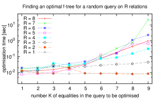
(a)

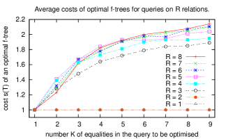
(b)

Figure 5: Experiment 1: Query optimisation on flat data, $K$ equalities on $R$ relations with $A=40$ attributes.

4.2 Exhaustive Search

To find an optimal f-plan for an equi-join query we search the space of all possible normalised f-trees and all possible operators between the f-trees (thus represented as a directed graph where f-trees are nodes and operators are edges). An f-plan for a given selection query $Q$ on an input over an f-tree $\mathcal{T}_{in}$ is any path $f$ from $\mathcal{T}_{in}$ to some final f-tree $\mathcal{T}_{final}$ such that (1) the equivalence classes of $\mathcal{T}_{final}$ are the classes of $\mathcal{T}_{in}$ joined by the query equalities.

The cost function $s(f)$ defines a distance function on the space of f-trees: the distance from $\mathcal{T}_{1}$ to $\mathcal{T}_{2}$ is the minimum possible cost $s(f)$ of an f-plan from $\mathcal{T}_{1}$ to $\mathcal{T}_{2}$. We are thus searching for f-trees $\mathcal{T}_{final}$ which satisfy (1), are closest to $\mathcal{T}_{in}$ (2), and have smallest possible cost (3). We can use Dijkstra’s algorithm to find distances of all f-trees from $\mathcal{T}_{in}$: explore the space starting with the $\mathcal{T}_{in}$ and trying all allowed operators, processing the reached f-trees in the order of increasing distance from $\mathcal{T}_{in}$. Then, among all f-trees satisfying (1), we pick one with the shortest distance from $\mathcal{T}_{in}$, and among these we pick one with smallest cost. Then we output a shortest path from $\mathcal{T}_{in}$ to this f-tree.

The complexity of the search is determined by the size of the search space. By successively applying operators to $\mathcal{T}_{in}$, we rearrange its nodes (swap operator) or merge pairs of its nodes (merge and absorb operators). For each partition of attributes over nodes, there will be a cluster of f-trees with the same nodes but different shape, among which we can move (transitively) using the swap operator. By applying a merge or absorb operator, we move to a cluster whose f-trees have one fewer node. Since we can never split a node in two, any valid f-plan will only merge nodes which end up merged in $\mathcal{T}_{final}$. For a query with $k$ equality selections, there are at most ${k+1\choose 2}=O(k^{2})$ pairs of nodes we may merge and we perform at most $k$ merges, so there are $O(k^{2k})$ reachable clusters. In a cluster with $m$ nodes there are at most $m^{m}$ f-trees. Since $m$ will be always at most the size $n$ of the initial f-tree $\mathcal{T}_{in}$, the size of the search space is $O(k^{2k}n^{n})$.

4.3 Greedy Heuristic

Our greedy optimisation algorithm restricts the search space for f-plans in two dimensions: (1) it only applies restructuring operators to nodes that participate in selection conditions, and (2) it considers a standard greedy approach to join ordering, whereby at each step it chooses a join with the least cost from the remaining joins.

The algorithm constructs an f-plan $f$ for a conjunction of equality conditions as follows. For each condition involving two attributes labelling nodes $\mathcal{A}$ and $\mathcal{B}$, we consider three possible restructuring scenarios: swapping one of the nodes $\mathcal{A}$ and $\mathcal{B}$ until $\mathcal{A}$ becomes the ancestor of $\mathcal{B}$ or the other way around, or bringing both $\mathcal{A}$ and $\mathcal{B}$ upwards until they become siblings. We choose the cheapest f-plan for each condition. This f-plan involves restructuring followed by a selection operator to perform the condition. We then order the conditions by the cost of their f-plans. The condition with the cheapest f-plan is performed first and its f-plan is appended to the overall f-plan $f$. We then repeat this process with the remaining conditions until we finish them. The new input f-tree is now the resulting f-tree of the f-plan of the previously chosen condition.

In contrast to the full search algorithm, this greedy algorithm takes only polynomial time in the size of the input f-tree $\mathcal{T}$. For each condition, there can be at most $O(|\mathcal{T}|)$ swaps and each swap requires to look at all descendants of the swapped nodes to check for independence. Computing the resulting f-tree in each of the three restructuring cases would then need $O(|\mathcal{T}|^{2})$.

5 Experimental Evaluation

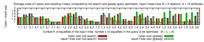
Figure 6: Experiment 2: Comparison of full-search and greedy query optimisers.

We evaluate the performance of our query engine FDB against three relational engines: one homebred in-memory (RDB) and two open-source engines (SQLite and PostgreSQL). Our main finding is that FDB clearly outperforms relational engines for data sets with many-to-many relationships. In particular, in our experiments we found that:

• The size of factorised query results is typically at most quadratic in the input size for queries of up to eight relations and nine join conditions (Figure 5 right).

• Finding optimal f-trees for queries of up to eight relations and six join conditions takes under 0.1 seconds (Figure 5 left). Finding optimal f-plans for queries on factorised data is about an order of magnitude slower. In contrast, the greedy optimiser takes under 5 ms (Figure 9) without any significant loss in the quality of factorisation (Figure 6).

• For queries on input relations, factorised query results are two to six orders of magnitude smaller than their flat equivalents and FDB outperforms RDB by up to four orders of magnitude (Figure 7). For the same workload SQLite performed about three times slower than RDB, and PostgreSQL performed three times slower than SQLite; both systems have additional overhead of fully functioning engines. Also, RDB implements a hand-crafted optimised query plan.

• The above observations hold for both uniform and Zipf data distributions, with a slightly larger gap in performance for the latter (Figure 7).

• The evaluation of subsequent queries on input data representing query results has the same time performance gap, since the new input is more succinct as factorised representation than as relation. Figure 8 compares evaluation times for selection queries on (1) one relation, which can be trivially evaluated by a single scan of this relation, and on (2) the factorisation of that relation, which may require restructuring.

• For one-to-many (e.g., key-foreign key) relationships, the performance gap is smaller, since the result sizes for one-to-many joins can only depend linearly on the input size and not quadratically as in the case of many-to-many joins and the possible gain brought by factorisation is less dramatic. For instance, in the TPC-H benchmark, the joins are predominantly on keys and therefore the sizes of the join results do not exceed that of the relation with foreign keys. Factorised query results are still more succinct than their relational representations, but only by a factor that is approximately the the number of relations in the query (experiments not plotted due to lack of space).

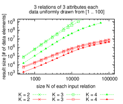
(a)

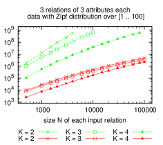
(b)

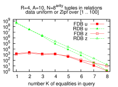
(c)

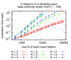
(d)

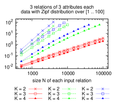
(e)

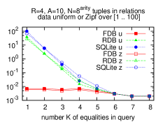
(f)

Figure 7: Experiment 3: Performance of query evaluation on flat relational data. For sizes (top row): FDB (solid red), RDB and SQLite and PostgreSQL (dashed green). For times (bottom row): FDB (solid red), RDB (dashed green), and SQLite (dotted blue); PostgreSQL is ca. 3 times slower than SQLite and not shown.

Competing Engines. We implemented FDB and RDB in C++ for execution in main memory, using the GLPK package v4.45 for solving linear programs. FDB evaluation and optimisation are described in previous sections. We also used the lightweight query engine SQLite 3.6.22 tuned for main memory operation by turning off the journal mode and synchronisations and by instructing it to use in-memory temporary store. Similarly, we run PostgreSQL 9.1 with the following parameters: fsync, synchronous commit, and full page writes are off, no background writer, shared buffers and working memory increased to 12 GB. Both SQLite and PostgreSQL read the data in their internal binary format, whereas FDB and RDB use the plain text format. The relations are given sorted; this allows RDB to use optimal relational join plans implemented as multi-way sort-merge joins. For all engines we report wall-clock times (averaged over five runs) to read data from disk and execute the query plans without writing the result to disk.

Experimental Setup. All experiments were performed on an Intel(R) Xeon(R) X5650 Quad 2.67GHz/64bit/32GB running VMWare VM with Linux 2.6.32/gcc4.4.5.

Experimental Design. The flow of our experiments is as follows. We generate random data and queries, then repeat a number of times four optimisation and evaluation experiments and report averages of optimisation time, execution time, representation sizes, and quality of produced f-plans.

We generate $R$ relations and distribute uniformly $A$ attributes over them. Each relation has a given number of tuples, each value is a natural number generated from 1 to $M$ using uniform or Zipf distribution. The queries are equi-joins over all of these relations. Their selections are conjunctions of $K$ non-redundant equalities.

For each generated query $Q$ and database $\mathbf{D}$, we do the following. In Experiment 1, we run the FDB optimiser to find an optimal f-tree $\mathcal{T}$ for the query result and report the optimisation time and the value of the parameter $s(Q)$ that controls the size of the f-representation of $Q(\mathbf{D})$ over $\mathcal{T}$. In Experiment 3, we compute the result $Q(\mathbf{D})$ using RDB, SQLite, and PostgreSQL, and the factorised query result using FDB. We then report on both the evaluation time and size of the result as the number of its singletons; a singleton holds an 8 byte integer.

In Experiments 2 and 4, we consider new queries on top of results produced in Experiments 1 and 3 respectively. The new queries are also equi-joins, where the selections are conjunctions of $L$ random (not already implied) equalities on attribute equivalence classes of $\mathcal{T}$.

For each new query $Q^{\prime}$, we run the FDB optimiser to find an optimal f-plan to compute the result and the resulting f-tree of the query result. In Experiment 2, we report the optimisation time and quality of the computed f-plans with the exhaustive and greedy optimisation algorithms; here, we consider the cost of the f-plan defined by the parameter $s(\cdot)$ of the intermediate and final f-trees; in our experiments, the alternative cost estimate discussed in Section 4.1 would lead to very similar choices of optimal f-plans. In Experiment 4, we execute the chosen f-plan with FDB and compute with the relational engines the selection conditions given by $Q^{\prime}$ on a single relation $Q(\mathbf{D})$ computed in Experiment 3. We report the execution times and query result sizes.

The parameters $K$ and $L$ are subject to $K+L<A$, as we can do at most $A-1$ non-trivial joins on $A$ attributes. We run the experiments five times for each parameter setting.

Experiment 1: Query optimisation on flat data.

Figure 5 shows average times for optimising a query on flat data, and average costs $s(\mathcal{T})$ for the chosen optimal f-tree $\mathcal{T}$ of the query result. For schemas with $A=40$ attributes over $R=1,\dots,8$ relations, we optimised queries of $K=1,\dots,9$ equality selections. The cost $s(\mathcal{T})$ of an optimal f-tree $\mathcal{T}$ is always $1$ for queries of up to two relations. For $R\geq 3$ and a sufficient number of joins we often get queries with optimal $s(\mathcal{T})=2$ and in very rare cases $s(\mathcal{T})>2$. This means that the sizes of f-representations for the query results are in most cases quadratic in the size of the input database even in the case of 9 equality selections on 8 relations. The optimiser searches a potentially exponentially large space of f-trees to find an optimal one, but runs under 1 second for queries with less than $8$ joins on up to $8$ relations.

Experiment 2: Query optimisation on factorised data.

Figure 6 shows the behaviour of query optimisation for factorised data. It shows the costs of the computed f-plans as well as the costs of the f-tree of the result computed by the f-plans for our full-search and greedy optimisation algorithms.

The queries under consideration have $L\leq 6$ joins on f-representations resulting after $K\leq 8$ joins on $R=4$ relations with $A=10$ attributes. The greedy optimiser gives optimal or nearly optimal results in most cases (by comparison with the optimal outcome of full search). The exceptions are queries joining most attributes of an f-representation produced by a query with few joins (small $K$, large $L$). In all cases the average f-plan cost is between 1 and 2, which means that the f-plans produce factorisations of at most quadratic size even though we join 4 relations. The results also show that for small queries (small $L$) the cost of the optimal f-plan is dominated by the cost of the final f-tree. As the query size (i.e., $L$) grows, the result f-tree has less attribute classes and its cost is smaller than the cost of the f-plan (i.e., smaller than the cost of intermediate f-trees that we must process while evaluating the query).

Figure 9 shows the execution times for both optimisers. The search space of possible f-trees grows exponentially with the number $L$ of selections and also with the size of the input f-tree (i.e., with decreasing $K$). The performance of the full-search algorithm is proportional to the size of the search space; we process about 1k f-trees/second. The greedy heuristic is polynomial in both $K$ and $L$, and in our scenario is 2-3 orders of magnitude faster than full search.

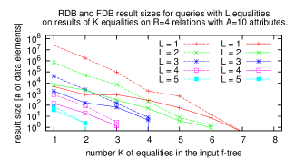
(a)

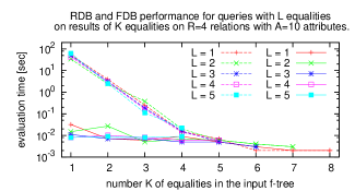
(b)

Figure 8: Experiment 4: Performance of FDB (solid lines) and RDB (dashed lines) for query evaluation on factorised data. RDB needs one scan over the input relation, whereas FDB may need restructuring the factorised input. The times and result sizes for SQLite and PostgreSQL are as for RDB and not plotted.

Experiment 3: Query evaluation on flat data.

We compared the performance of FDB, RDB, SQLite, and PostgreSQL for query evaluation on flat input data. Figure 7 shows the result sizes and evaluation times for queries with up to four equality selections on three ternary relations of increasing sizes in two settings: data generated using a uniform distribution over the range $[1,100]$ (left column) and using a more skewed, Zipf distribution (middle column).

The size gap between factorised and relational results is largest for queries with fewer equality selections, since the results are larger yet factorisable. The plots support the claim that the sizes are bounded by a power law, with a smaller exponent for FDB than for the relational engines.

The rightmost column in Figure 7 considers queries with four relations, two binary relations of size $8^{2}=64$ and two ternary relations of size $512=8^{3}$, whose values are drawn from $[1,20]$ using uniform and Zipf distributions. This dataset is combinatorial in nature. Each equality selection in the query decreases the number of result tuples by a constant factor of 20, which is exhibited in the flat result size produced by RDB. FDB factorises the up to 500M data values into less than 4k singletons for all considered queries.

The execution time for all engines is approximately proportional to their result sizes except for the millisecond region, where constant overhead dominates. SQLite performs consistently slightly worse than RDB, and PostgreSQL is about three times slower than SQLite. We used a timeout of 100 seconds, which prohibited the relational engines to complete in several cases (no plotted data points).

Experiment 4: Query evaluation on factorised data.

Figure 8 compares the performance of FDB and RDB for query evaluation on query results computed in Experiment 3 and with f-plans computed in Experiment 2. The behaviour of SQLite and PostgreSQL closely follows that of RDB.

FDB evaluates queries consisting of $L$ selections on factorised representations. The quality of the resulting factorisation is dictated by the quality of the f-plan. FDB uses the optimal f-plan found by the full-search optimiser. Additional experiments (not reported here) reveal that the f-plans found by the greedy optimiser can be up to 50% slower than the optimal f-plans. This is a good tradeoff, since the greedy optimiser runs fast even for large queries, while the full-search optimiser explores an exponential space.

RDB just evaluates a selection with a conjunction of $L$ equality conditions on the attributes of the input relation. This can be done in one scan over the input relation. For FDB, the cost of the f-plan may be non-trivial: the more the f-plan needs to unfold the f-representation, the more expensive the evaluation becomes. Figure 8 suggests that FDB only unfolds the f-representations to a small extent. Similar to query evaluation on flat data, FDB shows up to 4 orders of magnitude improvement over RDB for both evaluation time and result size. The gap closes once the size of the input data decreases to about 1000 tuples and both FDB and RDB perform in under 0.1 seconds.

Experiments 2 and 4 show that using f-representations for data processing is sustainable in the sense that the quality of factorisations, in particular their compactness and sizes, does not decay with the number of operations on the data.

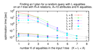
Figure 9: Experiment 2: Performance comparison of query optimisers. Slower series (top) correspond to full search, faster series (bottom) to greedy.

References

- [1] S. Abiteboul and N. Bidoit. Non first normal form relations: An algebra allowing data restructuring. JCSS, 33(3), 1986.
- [2] S. Abiteboul, R. Hull, and V. Vianu. Foundations of Databases. Addison-Wesley, 1995.
- [3] S. Agrawal, V. Narasayya, and B. Yang. Integrating vertical and horizontal partitioning into automated physical database design. In SIGMOD, 2004.
- [4] L. Antova, C. Koch, and D. Olteanu. Worlds and Beyond: Efficient Representation and Processing of Incomplete Information. In ICDE, 2007.
- [5] M. Aschinger, C. Drescher, G. Gottlob, P. Jeavons, and E. Thorstensen. Tackling the partner units configuration problem. In IJCAI, 2011.
- [6] G. Bagan, A. Durand, and E. Grandjean. On acyclic conjunctive queries and constant delay enumeration. In CSL, 2007.
- [7] P. A. Boncz, S. Manegold, and M. L. Kersten. Database architecture optimized for the new bottleneck: Memory access. In VLDB, 1999.
- [8] R. K. Brayton. Factoring logic functions. IBM J. Res. Develop., 31(2), 1987.
- [9] M. C. F. D. J. Abadi, S. R. Madden. Integrating compression and execution in column-oriented database systems. In SIGMOD, 2006.
- [10] G. Gottlob. On minimal constraint networks. In CP, 2011.
- [11] T. J. Green, G. Karvounarakis, and V. Tannen. Provenance semirings. In PODS, 2007.
- [12] M. Grohe and D. Marx. Constraint solving via fractional edge covers. In SODA, 2006.
- [13] M. Grund, J. Krüger, H. Plattner, A. Zeier, P. Cudré-Mauroux, and S. Madden. HYRISE - a main memory hybrid storage engine. PVLDB, 4(2), 2010.
- [14] T. Imielinski, S. Naqvi, and K. Vadaparty. Incomplete objects — a data model for design and planning applications. In SIGMOD, 1991.
- [15] S. I. Letovsky, R. W. Cottingham, C. J. Porter, and P. W. D. Li. GDB: The human genome database. Nucleic Acids Research, 26(1), 1998.
- [16] D. Olteanu and J. Huang. Using OBDDs for efficient query evaluation on probabilistic databases. In SUM, 2008.
- [17] D. Olteanu, C. Koch, and L. Antova. World-set decompositions: Expressiveness and efficient algorithms. TCS, 403(2-3), 2008.
- [18] D. Olteanu and J. Závodný. On factorisation of provenance polynomials. In TaPP, 2011.
- [19] D. Olteanu and J. Závodný. Factorised representations of query results: Size bounds and readability. In ICDT, 2012.
- [20] M. Pöss and D. Potapov. Data compression in Oracle. In VLDB, 2003.
- [21] R. Ramakrishnan and J. Gehrke. Database management systems. McGraw-Hill, 2003.
- [22] D. Suciu, D. Olteanu, C. Ré, and C. Koch. Probabilistic Databases. Synthesis Lectures on Data Management. Morgan & Claypool Publishers, 2011.