Functional renormalization group approach to the Ising-nematic quantum critical point of two-dimensional metals

Abstract

Using functional renormalization group methods, we study an effective low-energy model describing the Ising-nematic quantum critical point in two-dimensional metals. We treat both gapless fermionic and bosonic degrees of freedom on equal footing and explicitly calculate the momentum and frequency dependent effective interaction between the fermions mediated by the bosonic fluctuations. Following earlier work by S.-S. Lee for a one-patch model, Metlitski and Sachdev [Phys. Rev. B 82, 075127] recently found within a field-theoretical approach that certain three-loop diagrams strongly modify the one-loop results, and that the conventional $1/N$ expansion breaks down in this problem. We show that the singular three-loop diagrams considered by Metlitski and Sachdev are included in a rather simple truncation of the functional renormalization group flow equations for this model involving only irreducible vertices with two and three external legs. Our approximate solution of these flow equations explicitly yields the vertex corrections of this problem and allows us to calculate the anomalous dimension $\eta_{\psi}$ of the fermion field.

I Introduction

Inspired by the puzzling normal-state properties of the copper-oxide superconductors, the search for possible non-Fermi liquid states of metals continues to be a central topic in the theory of strongly correlated electrons. An interesting new clue toward an understanding of the cuprates and other materials comes from experiments on a variety of materials, indicating a nematic phase transition.Ando et al. (2002); Borzi et al. (2007); Kohsaka et al. (2007); Hinkov et al. (2008); Daou et al. (2010); Nandi et al. (2010); Fradkin et al. (2010) This is a quantum phase transition which, while preserving translational symmetry, breaks the lattice rotational symmetry from square to rectangular, i.e., the invariance under rotations of the system in the $x$-$y$ plane by $90^{\circ}$ is lost. At the quantum critical point, electrons couple strongly to order parameter fluctuations, leading to a destruction of the Fermi liquid state. The resulting distortion of the Fermi surface is also referred to as a Pomeranchuk transition.Pomeranchuk (1958); Halboth and Metzner (2000)

The conventional theoretical approach to quantum critical phenomena is the so-called Hertz-Millis approach, where the interaction between electrons is decoupled via a (bosonic) Hubbard-Stratonovich transformation and the fermionic degrees of freedom are integrated out.Hertz (1976); Millis (1993); Belitz et al. (2005); Löhneysen et al. (2007) However, as in the metallic state the electrons are gapless, this approach usually leads to singular vertices, which especially in low dimensions need to be treated with care. It can therefore be advantageous not to integrate out the fermions at all.

As concerns the nematic phase transition, the most effective scattering processes of electrons take place when the momentum of the bosons is locally almost tangential to the Fermi surface. The phase transition can therefore be modeled by coupling electrons in the vicinity of two patches of a Fermi surface to a gapless scalar Ising order parameter field. Indeed, the coupling of gapless fermions to gapless bosonic fluctuations is known to give rise to non-Fermi liquid behavior.Löhneysen et al. (2007); Vojta (2003) The corresponding field theory is very similar to a nonrelativistic gauge theory, which has been studied intensively,Holstein et al. (1973); Reizer (1989); Lee and Nagaosa (1992) starting with the important work by Holstein, Norton, and Pincus.Holstein et al. (1973) Such gauge theories have applications in a number of different problems, such as the description of the half-filled Landau level,Halperin et al. (1993) the description of spin liquids in terms of spinons which can form a critical spinon Fermi surface,Motrunich (2005); Lee and Lee (2005) or the description of the instability of a ferromagnetic quantum critical point.Rech et al. (2006) Similar gauge theories have also been used to describe fermions on a honeycomb lattice interacting through an electromagnetic gauge field.Gonzáles et al. (1994); Giuliani et al. (2010) In all cases, the low-energy behavior is expected to be described by a scale-invariant scaling theory. The single-particle Green function $G(\omega,\bm{k})$ was calculatedAltshuler et al. (1994); Polchinski (1994) for a spherical Fermi surface within the random phase approximation (RPA), resulting in

$$G(\omega+i0^{+},\bm{k})\propto\frac{1}{A_{\omega}|\omega|^{2/3}-\xi_{\bm{k}}}\;.$$ (1)

Here, $\omega$ and $\bm{k}$ are the frequency and momentum of the electron, $A_{\omega}=A^{\prime}\text{sgn}\left(\omega\right)+iA^{\prime\prime}$ is a complex constant depending on the sign of $\omega$, and $\xi_{\bm{k}}=v_{F}(|\bm{k}|-k_{F})$, where $v_{F}$ is the Fermi velocity and $k_{F}$ is the Fermi momentum, denotes the single-particle excitation energy. While the static part of the self-energy remains unrenormalized, its dynamic part implies that both the renormalized energy and damping rate of the electron scale in exactly the same way. Consequently, there are no well-defined sharp quasiparticles and Landau’s Fermi liquid theory breaks down.

For a long time, it was thought that the above scenario holds true when going beyond the RPA. Sedrakyan and Chubukov (2011) It was believed that this can be justified by considering the limit of large $N$, where $N$ is the number of fermion flavors. However, it was recently shown by LeeLee (2008, 2009) that, even if one considers only scattering processes in the vicinity of a single patch of the Fermi surface, the coupling to a gapless gauge field results in very strong correlations such that, even in the large-$N$ limit, the theory remains strongly coupled. Subsequently, Metlitski and SachdevMetlitski and Sachdev (2010a, b) considered a more realistic two-patch model where the two patches of the Fermi surface to which a given bosonic momentum is tangent are retained; they derived a scaling theory and explicitly calculated corrections to the bosonic and fermionic self-energies up to three loops, using the one-loop propagator in internal loop integrations. Metlitski and Sachdev identified certain three-loop contributions to the bosonic and fermionic self-energies (see Fig. 1), which give rise to logarithmically divergent corrections to the one-loop RPA results.

Figure 1: These three-loop diagrams have been identified by Metlitski and Sachdev Metlitski and Sachdev (2010a, b) to give singular corrections to the one-loop results for the bosonic and fermionic self-energies. Solid arrows denote the fermionic single-particle Green functions within the one-loop approximation, while wavy lines represent the RPA propagator of the bosonic fluctuations. The black dot is the bare interaction vertex between one boson and two fermion fields. The diagrams in (a) are three-loop corrections to the fermionic self-energy, while those in (b) represent corrections to the bosonic self-energy of the so-called Aslamazov-Larkin type.

Exponentiating these logarithmic terms, they obtained the following expression for the retarded propagator of the fermions,

$$G(\omega+i0^{+},\bm{k}) \propto \frac{1}{\left[A_{\omega}|\omega|^{1/z}-\xi_{\bm{k}}\right]^{1-\eta_{\psi}/2}},$$ (2)

where $\eta_{\psi}$ is the anomalous dimension of the fermion field and $z$ is the fermionic dynamic critical exponent. Using scaling relations for the fermionic and bosonic Green functions, Metlitski and Sachdev argued that the fermionic dynamic exponent is given by $z=z_{b}/2$, where $z_{b}$ is the corresponding bosonic dynamic exponent. Their explicit calculationsMetlitski and Sachdev (2010a) show that $z_{b}=3$ is not renormalized by fluctuations up to three loops, implying that $z=3/2$ is correctly given by the one-loop approximation. On the other hand, for the fermionic anomalous dimension, Metlitski and Sachdev obtain the finite result $\eta_{\psi}=0.068$ at the Ising-nematic transition, whereas $\eta_{\psi}=0$ within the one-loop approximation.

On a technical level, the reason for the breakdown of the large-$N$ expansion can be traced back to the fact that the curvature of the fermion propagator comes with a factor of $N$. This in combination with a cancellation of the curvature in a set of planar diagrams eventually leads to the breakdown of the large-$N$ expansion. In the words of Chubukov,Chubukov (2010) there is hidden one-dimensionality in two-dimensional systems.
Albeit $1/N$ can not be used as a control parameter, it was suggested by Mross et al.,Mross et al. (2010) following earlier work at finite $N$ by Nayak and Wilczek,Nayak and Wilczek (1994a); *Nayak94b to use $z_{b}$ as a tunable parameter. In this case it is possible to consider the limits $N\to\infty$ and $z_{b}-2\to 0$ while keeping the product $N(z_{b}-2)$ finite to bring the calculation under control. Using a tunable $z_{b}$ is a sensible strategy because a non-local interaction is not expected to be renormalized. Extrapolating the results obtained by Mross et al. Mross et al. (2010) to the physically relevant case $z_{b}=3$ and $N=2$, one obtains for the anomalous dimension of the fermion field $\eta_{\psi}\approx 0.6$ (using our definition (2) of $\eta_{\psi}$). Obviously, this value is much larger than the estimate $\eta_{\psi}\approx 0.068$ by Metlitski and Sachdev. Metlitski and Sachdev (2010a)

Even though the calculations in Refs. Metlitski and Sachdev, 2010a and Mross et al., 2010 are based on the field-theoretical renormalization group, the fact that two independent calculations involving different types of approximations produce different values for $\eta_{\psi}$ shows that on a quantitative level there are still open questions. Due to the sign problem in quantum Monte Carlo calculations and the fact that dynamical mean field theory can essentially only predict mean field exponents, the number of alternative methods to verify the correctness of the anomalous scaling properties of the Ising-nematic transition is limited. In this work, we study this problem by means of the one-particle irreducible implementation of the functional renormalization group (FRG) method,Wetterich (1993); Berges et al. (2002); Kopietz et al. (2010); Metzner et al. (2012) which is a modern implementation of the Wilsonian renormalization group idea. The flexibility of FRG methods to deal with systems involving both fermionic and bosonic fields has already been used by several authors.Baier et al. (2004, 2005); Schütz et al. (2005); Wetterich (2007); Strack et al. (2008); Bartosch et al. (2009a, b) In particular, in Refs. Schütz et al., 2005; Bartosch et al., 2009a, b it has been shown that it can be advantageous to introduce a cutoff parameter $\Lambda$ which regularizes the infrared divergences only in the momentum carried by the bosonic field (the momentum-transfer cutoff scheme). We show in this work that this cutoff scheme is also convenient to study the nematic quantum critical point.

The rest of this work is organized as follows. After introducing the model system and defining our notation in Sec. II, we give in Sec. III the FRG flow equations for the self-energies and vertex corrections in general form. We also introduce the momentum-transfer cutoff scheme and show that the singular three-loop diagrams shown in Fig. 1 are contained in a rather simple truncation of the hierarchy of FRG flow equations involving only irreducible two-point and three-point vertices. In Sec. IV, we show how to recover the known one-loop results for the momentum- and frequency-dependent fermionic and bosonic self-energies by integrating the FRG flow equations ignoring vertex corrections. In the main part of this work, given in Sec. V, we consider the system of FRG flow equations including vertex corrections. We explicitly calculate the effect of vertex corrections on the value of the fermionic anomalous dimension, $\eta_{\psi}$, to leading order in the small parameter $z_{b}-2$. In the concluding section VI, we summarize our results and discuss some open problems. We have added two appendices with more technical details. In Appendix A we derive skeleton equations relating the purely bosonic two-point and three-point functions to the fermionic propagators and irreducible vertices. These skeleton equations are useful to close the infinite hierarchy of FRG flow equations. Finally, in Appendix B, we explicitly evaluate the symmetrized fermionic loop with three external bosonic legs (the symmetrized three-loop vertex) for our model system.

II Definition of the model

We are interested in a minimal model describing the coupling of electrons in the proximity of a two-dimensional Fermi surface to a gapless scalar Bose field. In particular, the bosonic field can describe the fluctuations of a scalar order parameter near the onset of a metallic Ising-nematic phase, such as a $d$-wave nematic state in a two-dimensional square lattice, where the point-group symmetry of the lattice is reduced from square to rectangular. However, the gapless scalar Bose field can also describe the fluctuations of an emergent gauge field minimally coupled to a two-dimensional Fermi surface. For example, this can be physically realized in a system where a spin-liquid phase is described in terms of fermionic degrees of freedom (spinons), thereby causing the emergence of a $U(1)$ gauge symmetry in the system: The critical fluctuations near the onset of the spin-liquid phase are then described by the coupling of the spinon Fermi surface to the corresponding $U(1)$ gauge field. The general form of the action for our model can be written as $S=S_{\psi}+S_{\phi}+S_{\rm int}$, with

$$S_{\psi} = -\int_{K}\sum_{\sigma}(i\omega-\xi_{\bm{k}})\bar{\psi}_{K\sigma}\psi_{K\sigma},$$ (3)

$$S_{\phi} = \frac{1}{2}\int_{\bar{K}}\left(\rho_{0}+\tilde{\nu}_{0}\bar{\bm{k}}^{2}\right)\phi_{-\bar{K}}\phi_{\bar{K}},$$ (4)

$$S_{\rm int} = \int_{\bar{K}}\hat{O}_{\bar{K}}{[\bar{\psi},{\psi}]}\phi_{-\bar{K}},$$ (5)

where $\psi$ and $\phi$ denote two-dimensional Fermi and Bose fields, respectively, and $\hat{O}{[\bar{\psi},{\psi}]}$ is a bilinear operator in the fermion fields which has the same symmetry as the order parameter field $\phi$. In Eqs. (3)–(5), $K=(i\omega,\bm{k})$ denotes fermionic Matsubara frequency and two-dimensional momentum, while $\bar{K}=(i\bar{\omega},\bar{\bm{k}})$ denotes the corresponding bosonic quantities. The integration symbols are defined by $\int_{K}=(\beta V)^{-1}\sum_{\omega}\sum_{\bm{k}}$, and similarly for the bosonic quantities, where $\beta$ is the inverse temperature and $V$ is the volume. Throughout this work it is understood that we eventually take the zero temperature limit ($\beta\rightarrow\infty$) and the infinite volume limit ($V\rightarrow\infty$). The index $\sigma=1,\ldots,N$ labels $N$ different flavors of the fermion field. The fermionic energy dispersion $\xi_{\bm{k}}$ is defined relative to the Fermi energy $\epsilon_{F}$, i.e. $\xi_{\bm{k}}=\epsilon_{\bm{k}}-\epsilon_{F}$, while, in the bosonic dispersion, $\rho_{0}$ plays the role of a mass (or gap) term which measures the distance to the quantum critical point: At the quantum critical point, $\rho_{0}=0$, such that order parameter fluctuations become gapless. The absence of higher-order terms in $\phi$ and gradients of $\phi$ in the action defining our model can be justified by a dimensional analysis, which shows that such higher-order terms become irrelevant at the critical point.

In the general form given in Eqs. (3)–(5), the action of our model is still too complicated to be treated analytically with renormalization group or field-theoretical methods. However, as pointed out by Metlitski and SachdevMetlitski and Sachdev (2010a) (see also Ref. Sachdev, 2011), the relevant critical fluctuations can be described by a simplified minimal action involving only fermion fields with momenta close to two opposite patches on the Fermi surface. The reason is that the most singular scattering processes mediated by a given bosonic mode with momentum $\bar{\bm{k}}$ involve only fermions lying on patches of the Fermi surface which are almost tangential to the bosonic momentum $\bar{\bm{k}}$. The situation is shown graphically in Fig. 2, where the label $\alpha=\pm 1$ denotes the two patches of the Fermi surface which are tangential to a given bosonic mode with momentum parallel to $\bm{k}_{\perp}$ in the figure. In order to describe the singular behavior of the fermionic and bosonic Green functions at the critical point we can therefore restrict the general model involving fermions on the whole Fermi surface to a so-called two-patch model, characterized by the following Euclidean action:

$$S_{\rm patches}[\bar{\psi},\psi,\phi]=S_{0}[\bar{\psi},\psi]+S_{0}[\phi]+S_{1}[\bar{\psi},\psi,\phi],$$ (6)

$$S_{0}[\bar{\psi},\psi] = -\int_{K}\sum_{\alpha,\sigma}(i\omega-\xi^{\alpha}_{\bm{k}})\bar{\psi}^{\alpha}_{K\sigma}\psi^{\alpha}_{K\sigma},$$ (7)

$$S_{0}[\phi] = \frac{1}{2}\int_{\bar{K}}f^{-1}_{\bar{\bm{k}}}\phi_{-\bar{K}}\phi_{\bar{K}},$$ (8)

$$S_{1}[\bar{\psi},\psi,\phi] = \int_{K_{1}}\int_{K_{2}}\int_{\bar{K}_{3}}\sum_{\alpha,\sigma}\delta_{K_{1},K_{2}+\bar{K}_{3}}$$ (9)

$$\times\Gamma_{0}^{\bar{\psi}^{\alpha}\psi^{\alpha}\phi}(K_{1};K_{2};\bar{K}_{3})\bar{\psi}_{K_{1}\sigma}^{\alpha}\psi^{\alpha}_{K_{2}\sigma}\phi_{\bar{K}_{3}}.\hskip 19.91692pt$$

In the above expressions the fermion fields are now characterized by an additional upper index $\alpha=\pm 1$ labeling the two patches on the Fermi surface centered at the two opposite momenta $\bm{k}_{F}^{\alpha}=\alpha{\bm{k}}_{F}$, as shown in Fig. 2. By construction, the momenta of the fields characterizing the two-patch model are intended to lie in the vicinity of the Fermi momenta $\bm{k}_{F}^{\alpha}$, so that $|k_{\parallel}|$ and $|k_{\perp}|$ (the momenta relative to the Fermi momenta, as shown in Fig. 2) should be much smaller than $|{\bm{k}}_{F}|$. In particular, one should impose a cutoff, $\Lambda_{\perp}\sim k_{F}\Delta\theta$ on the momenta perpendicular to the Fermi surface normal, where $\Delta\theta$ is the angular extension of the patch. However, as long as integrals over such momenta turn out to be ultraviolet convergent, we can effectively send this cutoff to infinity without affecting the low-energy critical behavior of our theory.

Figure 2: The two-patch model considered in this work involves only two types of fermion fields with momenta close to two opposite patches on the Fermi surface centered at $\pm\bm{k}_{F}$. The fermionic momenta are measured locally with respect to $\pm\bm{k}_{F}$. We define $k_{\|}$ as the component of the momentum parallel to the local Fermi surface normal, and $k_{\bot}$ as the component orthogonal to the surface normal.

The energy dispersion relative to the true Fermi energy at patch $\alpha$ is assumed to be of the form

$$\xi^{\alpha}_{\bm{k}}=\epsilon_{\bm{k}_{F}^{\alpha}+\bm{k}}-\epsilon_{\bm{k}_{F}^{\alpha}}{=v_{F}^{\alpha}k_{\parallel}+\frac{k_{\bot}^{2}}{2m}}=\alpha v_{F}k_{\parallel}+\frac{k_{\bot}^{2}}{2m},$$ (10)

where $v_{F}$ is the Fermi velocity, $k_{\parallel}$ is the component of $\bm{k}$ parallel to the local normal to the Fermi surface, and $k_{\bot}$ is perpendicular to the local Fermi surface normal. In the last equality of Eq. (10) we have used the fact that the Fermi velocity has opposite sign at the two patches. We normalize the bosonic field $\phi_{\bar{K}}$ such that the bare fermion-boson interaction vertex $\Gamma_{0}^{\bar{\psi}^{\alpha}\psi^{\alpha}\phi}(K_{1};K_{2};\bar{K}_{3})$ is unity for the model describing the nematic quantum phase transition (which we discuss in detail below), and assumes the values $\alpha=\pm 1$ for the gauge field model, i.e.,

$$\Gamma_{0}^{\bar{\psi}^{\alpha}\psi^{\alpha}\phi}(K_{1};K_{2};\bar{K}_{3})=\Gamma_{0}^{\alpha}=\left\{\begin{array}[]{cl}1&\mbox{(nematic model),}\\ \alpha&\mbox{(gauge model).}\end{array}\right.$$ (11)

Finally, the coefficient of the quadratic term in the bosonic part of the action is assumed to be of the form

$$f^{-1}_{\bar{\bm{k}}}=\rho_{0}+\nu_{0}\left(\frac{|\bar{k}_{\bot}|}{2mv_{F}}\right)^{z_{b}-1},$$ (12)

where $\rho_{0}$ and $\nu_{0}$ are dimensionful constants with units of mass. (Recall that in two dimensions, the density of states also has units of mass.) We note that, for a nonspherical Fermi surface, $mv_{F}$ does not necessarily equal the Fermi momentum. For simplicity, in this work, we do not keep track of the renormalization of $\rho_{0}$ by fluctuations, so that we may set $\rho_{0}=0$ to describe the quantum critical point. We assume that the bosonic dynamic exponent $z_{b}$ is in the range $2<z_{b}\leq 3$. To construct a sensible limit of large $N$, the constants $\rho_{0}$ and $\nu_{0}$ should be proportional to $N$. However, according to Mross et al. Mross et al. (2010) the limit of large-$N$ can be safely taken only when $z_{b}-2$ is sent to zero simultaneously, such that the product $N(z_{b}-2)$ remains finite.

Although the FRG, unlike the field-theoretical renormalization group, does not rely on the presence of a small expansion parameter (which indeed is not present in the considered problem), it is convenient to express the above action in terms of rescaled dimensionless momenta, frequencies and fields, to carry out the renormalization group procedure. A general discussion of proper scaling in mixed Fermi-Bose systems can be found in Ref. Yamamoto and Si, 2010. Given an arbitrary momentum scale $\Lambda$, we define dimensionless fermionic labels $Q=(i\epsilon,q_{\parallel},q_{\bot})$ by setting

$$k_{\parallel} = \frac{\Lambda^{2}}{2mv_{F}}q_{\parallel},$$ (13a)

$$k_{\bot} = \Lambda q_{\bot},$$ (13b)

$$\omega = 2mv_{F}^{2}\left(\frac{\Lambda}{2mv_{F}}\right)^{z_{b}}\epsilon=\frac{\Lambda^{2}}{2m}\left(\frac{\Lambda}{2mv_{F}}\right)^{z_{b}-2}\epsilon.\hskip 19.91692pt$$ (13c)

The corresponding bosonic labels $\bar{Q}=(i\bar{\epsilon},\bar{q}_{\parallel},\bar{q}_{\bot})$ are defined in precisely the same way:

$$\bar{k}_{\parallel} = \frac{\Lambda^{2}}{2mv_{F}}\bar{q}_{\parallel},$$ (14a)

$$\bar{k}_{\bot} = \Lambda\bar{q}_{\bot},$$ (14b)

$$\bar{\omega} = 2mv_{F}^{2}\left(\frac{\Lambda}{2mv_{F}}\right)^{z_{b}}\bar{\epsilon}=\frac{\Lambda^{2}}{2m}\left(\frac{\Lambda}{2mv_{F}}\right)^{z_{b}-2}\bar{\epsilon}.\hskip 19.91692pt$$ (14c)

Introducing the rescaled dimensionless fields

$${\psi}^{\alpha}_{Q\sigma} = 4m^{2}v_{F}^{3}\left(\frac{\Lambda}{2mv_{F}}\right)^{\frac{z_{b}+5}{2}}\psi^{\alpha}_{K\sigma},$$ (15)

$${\phi}_{\bar{Q}} = 4m^{2}v_{F}^{2}\left(\frac{\Lambda}{2mv_{F}}\right)^{z_{b}+1}\phi_{\bar{K}},$$ (16)

the Euclidean action of our model can be written as

$$S_{0}[\bar{\psi},\psi] = -\int_{Q}\sum_{\alpha,\sigma}(i\zeta_{\Lambda}\epsilon-{\xi}^{\alpha}_{\bm{q}})\bar{\psi}^{\alpha}_{Q\sigma}\psi^{\alpha}_{Q\sigma},\hskip 34.1433pt$$ (17)

$$S_{0}[\phi] = \frac{1}{2}\int_{\bar{Q}}\left({r}_{\Lambda}+c_{0}|\bar{q}_{\bot}|^{z_{b}-1}\right)\phi_{-\bar{Q}}\phi_{\bar{Q}},$$ (18)

$$S_{1}[\bar{\psi},\psi,\phi] = \int_{Q_{1}}\int_{Q_{2}}\int_{\bar{Q}_{3}}\sum_{\alpha,\sigma}\delta_{Q_{1},Q_{2}+\bar{Q}_{3}}$$ (19)

$$\times {\Gamma}_{0}^{\bar{\psi}^{\alpha}\psi^{\alpha}\phi}(Q_{1};Q_{2};\bar{Q}_{3})\bar{\psi}_{Q_{1}\sigma}^{\alpha}\psi^{\alpha}_{Q_{2}\sigma}\phi_{\bar{Q}_{3}},\hskip 19.91692pt$$

where

$$\zeta_{\Lambda} = \left(\frac{\Lambda}{2mv_{F}}\right)^{z_{b}-2},$$ (20a)

$${\xi}^{\alpha}_{\bm{q}} = \alpha q_{\parallel}+q_{\bot}^{2},$$ (20b)

$${r}_{\Lambda} = \frac{\rho_{0}}{2m}\left(\frac{\Lambda}{2mv_{F}}\right)^{1-z_{b}},$$ (20c)

$$c_{0} = \frac{\nu_{0}}{2m},$$ (20d)

and the mixed fermion-boson vertex is the same as before,

$${\Gamma}_{0}^{\bar{\psi}^{\alpha}\psi^{\alpha}\phi}(Q_{1};Q_{2};\bar{Q}_{3})=\Gamma_{0}^{\bar{\psi}^{\alpha}\psi^{\alpha}\phi}(K_{1};K_{2};\bar{K}_{3})=\Gamma^{\alpha}_{0}.$$ (21)

If we use the expression $\nu_{0}=Nm/(2\pi)$ for the density of states of free fermions in two dimensions, we have $c_{0}=N/(4\pi)$. Consequently, setting $r_{\Lambda}\to 0$ to describe the quantum critical point, our model does not depend on any free parameters.
Our FRG procedure will generate also higher-order purely bosonic contributions to the effective action, which describe interactions between the boson fields, mediated by the fermions. In an expansion in powers of the fields, the lowest-order interaction process is cubic in the bosonic fields,

$$S_{3}[\phi] = \frac{1}{3!}\int_{\bar{K}_{1}}\int_{\bar{K}_{2}}\int_{\bar{K}_{3}}\delta_{\bar{K}_{1}+\bar{K}_{2}+\bar{K}_{3},0}$$ (22)

$$\times\Gamma^{\phi\phi\phi}(\bar{K}_{1},\bar{K}_{2},\bar{K}_{3})\phi_{\bar{K}_{1}}\phi_{\bar{K}_{2}}\phi_{\bar{K}_{3}}$$

$$= \frac{1}{3!}\int_{\bar{Q}_{1}}\int_{\bar{Q}_{2}}\int_{\bar{Q}_{3}}\delta_{\bar{Q}_{1}+\bar{Q}_{2}+\bar{Q}_{3},0}$$

$$\times\tilde{\Gamma}^{\phi\phi\phi}(\bar{Q}_{1},\bar{Q}_{2},\bar{Q}_{3})\phi_{\bar{Q}_{1}}\phi_{\bar{Q}_{2}}\phi_{\bar{Q}_{3}},$$

with

$$\tilde{\Gamma}^{\phi\phi\phi}(\bar{Q}_{1},\bar{Q}_{2},\bar{Q}_{3}) = v_{F}^{2}\left(\frac{\Lambda}{2mv_{F}}\right)^{3-z_{b}}\Gamma^{\phi\phi\phi}(\bar{K}_{1},\bar{K}_{2},\bar{K}_{3}).$$

Although for $z_{b}<3$ this vertex seems to be irrelevant by power counting, it turns out that it has a singular dependence on the external momenta and frequencies and therefore cannot be neglected. Because, within our bosonic momentum-transfer cutoff scheme, all vertices involving only bosonic external legs are finite at the initial renormalization group scale,Schütz et al. (2005); Kopietz et al. (2010) it is crucial to keep track of the FRG flow of the vertex $\Gamma^{\phi\phi\phi}(\bar{K}_{1},\bar{K}_{2},\bar{K}_{3})$. In this work, we do this by means of a skeleton equation relating $\Gamma^{\phi\phi\phi}(\bar{K}_{1},\bar{K}_{2},\bar{K}_{3})$ to the symmetrized fermion loop with three external bosonic legs and renormalized fermionic propagators, as discussed in Appendix A. An explicit evaluation of this vertex is given in Appendix B.

If we identify $\Lambda$ with the renormalization group flow parameter which is reduced under the renormalization group procedure, the canonical dimensions of all quantities explicitly appear in the FRG flow equations with the above rescaling. To compare the FRG results with perturbation theory, it is more convenient, however, not to include the canonical dimensions into the definition of the vertices. Therefore, we simply choose $\Lambda=2mv_{F}$ in the above expressions, so that $\zeta_{\Lambda}\rightarrow 1$ and $r_{\Lambda}\rightarrow r_{0}=\rho_{0}/(2m)$. Renaming again $Q\rightarrow K$, our bare action is then the sum of the following three terms,

$$S_{0}[\bar{\psi},\psi] = -\int_{K}\sum_{\alpha,\sigma}(i\omega-\xi^{\alpha}_{\bm{k}})\bar{\psi}^{\alpha}_{K\sigma}\psi^{\alpha}_{K\sigma},$$ (24)

$$S_{0}[\phi] = \frac{1}{2}\int_{\bar{K}}(r_{0}+c_{0}|\bar{k}_{\bot}|^{z_{b}-1})\phi_{-\bar{K}}\phi_{\bar{K}},$$ (25)

$$S_{1}[\bar{\psi},\psi,\phi] = \int_{K_{1}}\int_{K_{2}}\int_{\bar{K}_{3}}\sum_{\alpha,\sigma}\delta_{K_{1},K_{2}+\bar{K}_{3}}$$ (26)

$$\times \Gamma_{0}^{\bar{\psi}^{\alpha}\psi^{\alpha}\phi}(K_{1};K_{2};\bar{K}_{3})\bar{\psi}_{K_{1}\sigma}^{\alpha}\psi^{\alpha}_{K_{2}\sigma}\phi_{\bar{K}_{3}},\hskip 19.91692pt$$

where now

$$\xi^{\alpha}_{\bm{k}}=\alpha k_{\parallel}+k_{\bot}^{2},\;\ \;\;r_{0}=\frac{\rho_{0}}{2m},\;\;\;c_{0}=\frac{\nu_{0}}{2m}.$$ (27)

The corresponding Gaussian propagators are

$$G_{0}^{\alpha}(K) = \frac{1}{i\omega-\xi^{\alpha}_{\bm{k}}}=\frac{1}{i\omega-\alpha k_{\parallel}-k_{\bot}^{2}},$$ (28)

$$F_{0}(\bar{K}) = f_{\bar{\bm{k}}}=\frac{1}{r_{0}+c_{0}|\bar{k}_{\bot}|^{z_{b}-1}}.$$ (29)

This dimensionless parametrization of our model is what is used in the following sections.

III FRG flow equations

The starting point of our calculation is the Wetterich equation Wetterich (1993); Berges et al. (2002) for the coupled Fermi-Bose model defined above, which is an exact FRG flow equation for the generating functional $\Gamma_{\Lambda}[\bar{\psi},\psi,\phi]$ of the one-line irreducible vertices of our theory. This flow equation describes the exact evolution of $\Gamma_{\Lambda}[\bar{\psi},\psi,\phi]$ as some (now dimensionless) cutoff parameter $\Lambda$ is reduced. By expanding $\Gamma_{\Lambda}[\bar{\psi},\psi,\phi]$ in powers of the fields, we obtain an infinite hierarchy of coupled integro-differential equations for the one-line irreducible vertices of our model. This hierarchy is formally exact, but, in practice, further approximations are usually necessary in order to obtain explicit results for the vertex functions (see Refs. Kopietz et al., 2010; Metzner et al., 2012 for recent reviews). Moreover, the proper choice of the cutoff scheme is also very important.

For our effective low-energy model discussed above, it is, in principle, possible to introduce cutoffs in both the bosonic and the fermionic sectors and regularize the inverse Gaussian propagators as follows:

$${[}F_{0,\Lambda}(\bar{K})]^{-1} = f^{-1}_{\bar{\bm{k}}}+\bar{R}_{\Lambda}(\bar{{K}}),$$ (30)

$${[}G^{\alpha}_{0,\Lambda}(K)]^{-1} = i\omega-\xi^{\alpha}_{\bm{k}}-R_{\Lambda}(K).$$ (31)

For the calculations in the present problem, we find it more convenient to introduce a sharp momentum-transfer cutoff only in the bosonic sector. Using a similar cutoff procedure, two of us were able to derive the exact scaling behavior of the Tomonaga-Luttinger model within an FRG approach.Schütz et al. (2005) We therefore set $R_{\Lambda}(K)=0$ in the fermionic sector, and choose

$$\bar{R}_{\Lambda}(\bar{{K}})=f^{-1}_{\bar{\bm{k}}}\left[\Theta^{-1}(|\bar{k}_{\bot}|-\Lambda)-1\right]$$ (32)

for the boson cutoff. This leads to the cutoff-dependent bare Gaussian propagator

$$F_{0,\Lambda}(\bar{K})=\Theta(|\bar{k}_{\bot}|-\Lambda)f_{\bar{\bm{k}}},$$ (33)

which vanishes for $|\bar{k}_{\bot}|<\Lambda$ and equals $f_{\bar{\bm{k}}}$ for $|\bar{k}_{\bot}|>\Lambda$. As there is no cutoff function in the fermionic sector, all purely fermionic loops already have non-vanishing initial values at the beginning of the flow. We see explicitly below that these are highly singular and need to be treated with care.

The exact hierarchy of FRG flow equations for the one-line irreducible vertices of our model can be obtained as a special case of the general hierarchy of FRG flow equations for mixed Bose-Fermi theories written down in Refs. Schütz et al., 2005; Kopietz et al., 2010. For our purpose, it is sufficient to consider a truncation of this hierarchy which generates, after iteration (apart from many other diagrams), the important three-loop diagrams identified by Metlitski and Sachdev,Metlitski and Sachdev (2010a) shown in Fig. 1. Our truncation is characterized by the following three points.

• On the right-hand side of the flow equations for the fermionic and bosonic self-energies, retain only contributions involving irreducible vertices with three external legs.

• Renormalize all three-legged vertices by triangular diagrams involving all combinations of three-legged vertices.

• On the right-hand side of the flow equations for all three-legged vertices, approximate the vertex with one bosonic and two fermionic external legs by its bare value.

Let us now explicitly give the corresponding FRG flow equations. The fermionic self-energy $\Sigma^{\alpha}(K)$ and bosonic self-energy $\Pi(\bar{K})$ satisfy the flow equations

$$\partial_{\Lambda}{\Sigma}^{\alpha}(K) = \int_{\bar{K}}\left[\dot{F}(\bar{K})G^{\alpha}(K+\bar{K})+{F}(\bar{K})\dot{G}^{\alpha}(K+\bar{K})\right]\Gamma^{\bar{\psi}^{\alpha}\psi^{\alpha}\phi}(K+\bar{K};K;\bar{K})\Gamma^{\bar{\psi}^{\alpha}\psi^{\alpha}\phi}(K;K+\bar{K};-\bar{K}),\hskip 19.91692pt$$ (34)

$$\partial_{\Lambda}{\Pi}(\bar{K}) = \int_{K}\sum_{\alpha,\sigma}\left[\dot{G}^{\alpha}(K)G^{\alpha}(K+\bar{K})+{G}^{\alpha}(K)\dot{G}^{\alpha}(K+\bar{K})\right]\Gamma^{\bar{\psi}^{\alpha}\psi^{\alpha}\phi}(K+\bar{K};K;\bar{K})\Gamma^{\bar{\psi}^{\alpha}\psi^{\alpha}\phi}(K;K+\bar{K};-\bar{K})$$ (35)

$$- \int_{\bar{K}^{\prime}}\dot{F}(\bar{K}^{\prime})F(\bar{K}^{\prime}+\bar{K})\Gamma^{\phi\phi\phi}(\bar{K},\bar{K}^{\prime},-\bar{K}-\bar{K}^{\prime})\Gamma^{\phi\phi\phi}(-\bar{K},-\bar{K}^{\prime},\bar{K}+\bar{K}^{\prime}),$$

which are shown graphically in Fig. 3 for a general cutoff scheme. Here the scale-dependent bosonic and fermionic propagators are

$$F(\bar{K}) = \frac{1}{[F_{0,\Lambda}(\bar{K})]^{-1}+\Pi(\bar{K})},$$ (36)

$$G^{\alpha}(K) = \frac{1}{[G^{\alpha}_{0,\Lambda}(K)]^{-1}-\Sigma^{\alpha}(K)},$$ (37)

while the corresponding single-scale propagators are

$$\dot{F}(\bar{K}) = -F^{2}(\bar{K})\partial_{\Lambda}[F_{0,\Lambda}(\bar{K})]^{-1},$$ (38)

$$\dot{G}^{\alpha}(K) = -[G^{\alpha}(K)]^{2}\partial_{\Lambda}[G^{\alpha}_{0,\Lambda}(K)]^{-1}.$$ (39)

Note that in the momentum-transfer cutoff scheme $\dot{G}^{\alpha}(K)=0$ such that we should omit all diagrams involving fermionic single-scale propagators. With a sharp cutoff in the bosonic transverse momentum, the full bosonic propagator is

$$F_{\Lambda}(\bar{K})=\frac{\Theta(|\bar{k}_{\bot}|-\Lambda)}{r_{0}+c_{0}|\bar{k}_{\bot}|^{z_{b}-1}+\Theta(|\bar{k}_{\bot}|-\Lambda)\Pi_{\Lambda}(\bar{K})},$$ (40)

while the corresponding single-scale propagator is given by

$$\dot{F}_{\Lambda}(\bar{K})=-\frac{\delta(|\bar{k}_{\bot}|-\Lambda)}{r_{0}+c_{0}\Lambda^{z_{b}-1}+\Pi_{\Lambda}(\bar{K})}.$$ (41)

The right-hand sides of Eqs. (34) and (35) also depend on the one-line irreducible three-point vertex with two fermionic and one bosonic external legs, $\Gamma^{\bar{\psi}^{\alpha}\psi^{\alpha}\phi}(K+\bar{K};K;\bar{K})$, and on the one-line irreducible three-point vertex with three bosonic external legs, $\Gamma^{\phi\phi\phi}(\bar{K},\bar{K}^{\prime},-\bar{K}-\bar{K}^{\prime})$, where the superscripts indicate the fields associated with the energy-momentum labels. Within our truncation, the flow of $\Gamma^{\bar{\psi}^{\alpha}\psi^{\alpha}\phi}$ is determined by the following flow equation,

$$\partial_{\Lambda}{\Gamma}^{\bar{\psi}^{\alpha}\psi^{\alpha}\phi}(K+\bar{K};K;\bar{K}) = \int_{\bar{K}^{\prime}}\Bigl{[}\dot{F}(\bar{K}^{\prime})G^{\alpha}(K+\bar{K}^{\prime})G^{\alpha}(K+\bar{K}+\bar{K}^{\prime})+{F}(\bar{K}^{\prime})\dot{G}^{\alpha}(K+\bar{K}^{\prime})G^{\alpha}(K+\bar{K}+\bar{K}^{\prime})$$ (42)

$$\hskip 14.22636pt+{F}(\bar{K}^{\prime})G^{\alpha}(K+\bar{K}^{\prime})\dot{G}^{\alpha}(K+\bar{K}+\bar{K}^{\prime})\Bigr{]}\Gamma^{\bar{\psi}^{\alpha}\psi^{\alpha}\phi}(K+\bar{K}^{\prime};K;\bar{K}^{\prime})$$

$$\hskip 14.22636pt\times\Gamma^{\bar{\psi}^{\alpha}\psi^{\alpha}\phi}(K+\bar{K};K+\bar{K}+\bar{K}^{\prime};-\bar{K}^{\prime})\Gamma^{\bar{\psi}^{\alpha}\psi^{\alpha}\phi}(K+\bar{K}+\bar{K}^{\prime};K+\bar{K}^{\prime};\bar{K})$$

$$- \int_{\bar{K}^{\prime}}\Bigl{[}\dot{F}(\bar{K}^{\prime})F(\bar{K}+\bar{K}^{\prime})G^{\alpha}(K+\bar{K}+\bar{K}^{\prime})+{F}(\bar{K}^{\prime})\dot{F}(\bar{K}+\bar{K}^{\prime})G^{\alpha}(K+\bar{K}+\bar{K}^{\prime})$$

$$\hskip 14.22636pt+{F}(\bar{K}^{\prime}){F}(\bar{K}+\bar{K}^{\prime})\dot{G}^{\alpha}(K+\bar{K}+\bar{K}^{\prime})\Bigr{]}\Gamma^{\phi\phi\phi}(-\bar{K}-\bar{K}^{\prime},\bar{K},\bar{K}^{\prime})$$

$$\hskip 14.22636pt\times\Gamma^{\bar{\psi}^{\alpha}\psi^{\alpha}\phi}(K+\bar{K};K+\bar{K}+\bar{K}^{\prime};-\bar{K}^{\prime})\Gamma^{\bar{\psi}^{\alpha}\psi^{\alpha}\phi}(K+\bar{K}+\bar{K}^{\prime};K;\bar{K}+\bar{K}^{\prime}).$$

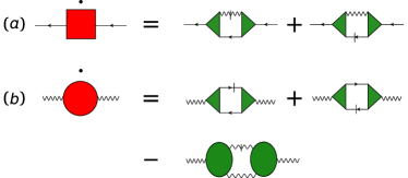
Figure 3: (Color online) (a) Graphical representation of the FRG flow equation (34) for the fermionic self-energy $\Sigma^{\alpha}(K)$, which is represented by a shaded rectangle with one incoming arrow associated with $\psi^{\alpha}_{K\sigma}$, and one outgoing arrow associated with $\bar{\psi}^{\alpha}_{K\sigma}$. The shaded triangles represent the three-legged vertex $\Gamma^{\bar{\psi}^{\alpha}\psi^{\alpha}\phi}(K+\bar{K};K;\bar{K})$ with two fermionic and one bosonic external legs. The boson propagator is represented by a wavy line. The black dot above the rectangle denotes a derivative with respect to the flow parameter, while the slashes attached to the propagators on the right-hand side denote the corresponding single-scale propagators. (b) Graphical representation of the FRG flow equation (35) for the bosonic self-energy $\Pi(\bar{K})$. The shaded circles on the right-hand side represent the symmetrized bosonic three-point vertex. Note that, in the momentum-transfer cutoff scheme, all diagrams with a slash on internal fermionic propagators should be omitted.

A graphical representation of this flow equation is shown in Fig. 4. In the momentum-transfer cutoff scheme, we should omit, again, all terms involving the fermionic single-scale propagator. Finally, the flow equation for the symmetrized bosonic three-legged vertex is

$$\partial_{\Lambda}{\Gamma}^{\phi\phi\phi}(\bar{K}_{1},\bar{K}_{2},-\bar{K}_{1}-\bar{K}_{2})$$ (43)

$$= \int_{\bar{K}}\bigl{[}\dot{F}(\bar{K})F(\bar{K}-\bar{K}_{1})F(\bar{K}+\bar{K}_{2})+{F}(\bar{K})\dot{F}(\bar{K}-\bar{K}_{1})F(\bar{K}+\bar{K}_{2})+{F}(\bar{K})F(\bar{K}-\bar{K}_{1})\dot{F}(\bar{K}+\bar{K}_{2})\bigr{]}$$

$$\hskip 14.22636pt\times\Gamma^{\phi\phi\phi}(\bar{K}_{1},\bar{K}-\bar{K}_{1},-\bar{K})\Gamma^{\phi\phi\phi}(\bar{K}_{2},-\bar{K}-\bar{K}_{2},\bar{K})\Gamma^{\phi\phi\phi}(-\bar{K}_{1}-\bar{K}_{2},-\bar{K}+\bar{K}_{1},\bar{K}+\bar{K}_{2})$$

$$+ \int_{K}\sum_{\alpha,\sigma}\Bigl{\{}\bigl{[}\dot{G}^{\alpha}({K})G^{\alpha}({K}+\bar{K}_{1})G^{\alpha}({K}+\bar{K}_{1}+\bar{K}_{2})+{G}^{\alpha}({K})\dot{G}^{\alpha}({K}+\bar{K}_{1})G^{\alpha}({K}+\bar{K}_{1}+\bar{K}_{2})$$

$$\hskip 36.98857pt+{G}^{\alpha}({K})G^{\alpha}({K}+\bar{K}_{1})\dot{G}^{\alpha}({K}+\bar{K}_{1}+\bar{K}_{2})\bigr{]}\Gamma^{\bar{\psi}^{\alpha}\psi^{\alpha}\phi}(K+\bar{K}_{1};K;\bar{K}_{1})\Gamma^{\bar{\psi}^{\alpha}\psi^{\alpha}\phi}(K+\bar{K}_{1}+\bar{K}_{2};K+\bar{K}_{1};\bar{K}_{2})$$

$$\hskip 45.5244pt\times\Gamma^{\bar{\psi}^{\alpha}\psi^{\alpha}\phi}(K;K+\bar{K}_{1}+\bar{K}_{2};-\bar{K}_{1}-\bar{K}_{2})+(\bar{K}_{1}\leftrightarrow\bar{K}_{2})\Bigr{\}},$$

which is shown graphically in Fig. 5.

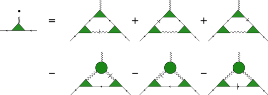
Figure 4: (Color online) Graphical representation of the FRG flow equation (42) for the three-legged vertex $\Gamma^{\bar{\psi}^{\alpha}\psi^{\alpha}\phi}(K;K^{\prime};\bar{K})$ with two fermionic and one bosonic external legs.

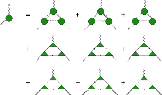
Figure 5: (Color online) Graphical representation of the FRG flow equation (43) for the three-legged boson vertex $\Gamma^{\phi\phi\phi}(\bar{K}_{1},\bar{K}_{2},\bar{K}_{3})$.

If we ignore the vertex with three bosonic external legs, the above system of FRG flow equations has already been written down in Ref. Schütz et al., 2005 (see also Ref. Kopietz et al., 2010). Although the above flow equations involve only one-loop integrations, the iterative solution of these equations generates higher-loop diagrams. In particular, the singular three-loop diagrams shown in Fig. 1 are generated as follows: The Aslamazov-Larkin type of contribution to the bosonic self-energy shown in Fig. 1 (b) is generated by the last six diagrams on the right-hand side of the flow equation for $\Gamma^{\phi\phi\phi}(\bar{K}_{1},\bar{K}_{2},\bar{K}_{3})$ shown in Fig. 5 after integrating this flow equation over the flow parameter and substituting the result into the right-hand side of the flow equation for $\Pi(\bar{K})$ shown in Fig. 3 (b). The singular fermionic three-loop diagram in Fig. 1 (a) is generated by substituting the same contribution to $\Gamma^{\phi\phi\phi}(\bar{K}_{1},\bar{K}_{2},\bar{K}_{3})$ into the flow equation for $\Gamma^{\bar{\psi}^{\alpha}\psi^{\alpha}\phi}(K;K^{\prime};\bar{K})$ shown in Fig. 4. After integrating the resulting flow equation again over $\Lambda$ and substituting the resulting vertex correction into the right-hand side of the flow equation for $\Sigma^{\alpha}(K)$ shown in Fig. 3 (a), we generate the Metlitski-Sachdev diagrams shown in Fig. 1 (a). In fact, there are even further contributions, e.g. using the renormalized vertex $\Gamma^{\bar{\psi}^{\alpha}\psi^{\alpha}\phi}\left(K;K^{\prime};\bar{K}\right)$ containing the vertex $\Gamma^{\phi\phi\phi}(\bar{K}_{1},\bar{K}_{2},\bar{K}_{3})$ as depicted in the second line of Fig. 4 also gives rise to an Aslamazov-Larkin contribution when substituted into the diagram on the right-hand side of Fig. 3 (b).

Although Eqs. (34)–(43) form a closed system of integro-differential equations for the two-point and three-point functions of our model, a direct numerical solution of these equations seems to be prohibitively difficult, so that further approximations are necessary. As a first simplification, we use, below, truncated skeleton equations instead of the FRG flow equations (35) and (43) to determine the bosonic self-energy $\Pi(\bar{K})$ and three-point vertex $\Gamma^{\phi\phi\phi}(\bar{K}_{1},\bar{K}_{2},\bar{K}_{3})$. As discussed in Appendix A, the Dyson-Schwinger equations of motion imply exact skeleton equations relating $\Pi(\bar{K})$ and $\Gamma^{\phi\phi\phi}(\bar{K}_{1},\bar{K}_{2},\bar{K}_{3})$ to the fermionic propagators, the three-point vertex $\Gamma^{\bar{\psi}^{\alpha}\psi^{\alpha}\phi}(K;K^{\prime};\bar{K})$ with two fermionic and one bosonic external legs and the mixed four-point vertex $\Gamma^{\bar{\psi}\psi\phi\phi}(K;K^{\prime};\bar{K}_{1};\bar{K}_{2})$ (see Eqs. (A1) and (A3)).

IV Truncation without vertex corrections

In this section, we show how the known one-loop results for the self-energies can be obtained within our FRG approach if we neglect vertex corrections. Keeping in mind that, in the momentum-transfer cutoff scheme, we do not introduce any cutoff in the fermionic sector, the scale-dependent fermionic propagator is

$$G^{\alpha}_{\Lambda}(K)=\frac{1}{i\omega-\xi^{\alpha}_{\bm{k}}-[\Sigma^{\alpha}_{\Lambda}(K)-\Sigma^{\alpha}_{\Lambda}(0)]},$$ (44)

where $\Sigma_{\Lambda}^{\alpha}(0)$ is the self-energy at the renormalized flowing Fermi surface. The subtraction of $\Sigma_{\Lambda}^{\alpha}(0)$ is necessary because, by assumption, we have expanded the wave vector at the renormalized Fermi surface of the underlying model. Given the cutoff-dependent self-energy $\Sigma_{\Lambda}(K)$, we may define the Fermi surface for a given value of the cutoff parameter $\Lambda$ via

$$\epsilon_{\bm{k}_{F}}+\Sigma_{\Lambda}(i0,\bm{k}_{F}^{\alpha})=\mu,$$ (45)

which, for $\Lambda\rightarrow 0$, reduces to the definition of the true Fermi surface. Hence, we may write

$$\epsilon_{\bm{k}_{F}^{\alpha}+\bm{k}}-\mu=\epsilon_{\bm{k}_{F}^{\alpha}+\bm{k}}-\epsilon_{\bm{k}_{F}^{\alpha}}-\Sigma_{\Lambda}(i0,\bm{k}_{F}^{\alpha})=\xi^{\alpha}_{\bm{k}}-\Sigma^{\alpha}_{\Lambda}(0).$$ (46)

Following Refs. Bartosch et al., 2009a, b; Isidori et al., 2010, we now use the skeleton equation (A1) to determine the flowing bosonic self-energy. Using the fact that $(\Gamma_{0}^{\alpha})^{2}=1$, the scale-dependent bosonic self-energy is thus given by

$$\Pi_{\Lambda}(\bar{K})=\frac{1}{2}\int_{K}\sum_{\alpha,\sigma}G^{\alpha}_{\Lambda}(K)\left[G^{\alpha}_{\Lambda}(K+\bar{K})+G^{\alpha}_{\Lambda}(K-\bar{K})\right],$$ (47)

while the fermionic self-energy satisfies the FRG flow equation

$$\partial_{\Lambda}\Sigma^{\alpha}_{\Lambda}(K)=\int_{\bar{K}}\dot{F}_{\Lambda}(\bar{K})G^{\alpha}_{\Lambda}(\bar{K}+K).$$ (48)

A graphical representation of Eqs. (47) and (48) is shown in Fig. 6.

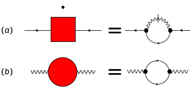
Figure 6: (Color online) (a) Graphical representation of the FRG flow equation (48) for the fermionic self-energy in the momentum-transfer cutoff scheme in the simplest approximation where the three-legged vertex is approximated by its bare value (represented by a black dot). (b) Truncated skeleton equation (47) for the bosonic self-energy.

Actually, the integral on the right-hand side of Eq. (48) is ultraviolet divergent for our model, but since we do not keep track of the shape of the renormalized Fermi surface, we can instead consider the subtracted self-energy,

$$\Delta^{\alpha}_{\Lambda}(K)=\Sigma^{\alpha}_{\Lambda}(K)-\Sigma^{\alpha}_{\Lambda}(0),$$ (49)

which appears in our cutoff-dependent fermionic propagator (44). The subtracted self-energy then satisfies the FRG flow equation

$$\partial_{\Lambda}{\Delta}^{\alpha}_{\Lambda}(K)=\int_{\bar{K}}\dot{F}_{\Lambda}(\bar{K})\left[G^{\alpha}_{\Lambda}(\bar{K}+K)-G^{\alpha}_{\Lambda}(\bar{K})\right].$$ (50)

To obtain an approximate solution of this flow equation, we expand the subtracted self-energy for small momenta and frequencies,

$${\Delta}^{\alpha}_{\Lambda}(K)=-(Z_{\Lambda}^{-1}-1)i\omega+(\tilde{Z}_{\Lambda}^{-1}-1)\xi^{\alpha}_{\bm{k}}+\ldots,$$ (51)

where we have used the fact that the $\bm{k}$-dependence of the self-energy appears only in the combination $\xi^{\alpha}_{\bm{k}}$. Because the cutoff, $\Lambda$, regularizes the singularity of the bare interaction, the self-energy is analytic for small momenta and frequencies and can hence be expanded into a Taylor series. The corresponding low-energy approximation for the fermion propagator is

$$G^{\alpha}_{\Lambda}(K)=\frac{1}{Z_{\Lambda}^{-1}i\omega-\tilde{Z}_{\Lambda}^{-1}\xi^{\alpha}_{\bm{k}}}=\frac{Z_{\Lambda}}{i\omega-(Z_{\Lambda}/\tilde{Z}_{\Lambda})\xi^{\alpha}_{\bm{k}}}.$$ (52)

Substituting Eq. (52) into Eq. (47), it is convenient to first perform the integration over $k_{\parallel}$,Metlitski and Sachdev (2010a) which can be done using the residue theorem,

$$\Pi_{\Lambda}(\bar{K}) = \frac{N}{2}Z_{\Lambda}\tilde{Z}_{\Lambda}\int\frac{dk_{\bot}}{2\pi}\sum_{\alpha}\frac{i\alpha}{i\bar{\omega}-(Z_{\Lambda}/\tilde{Z}_{\Lambda})(\alpha\bar{k}_{\parallel}+\bar{k}_{\bot}^{2}+2\bar{k}_{\bot}k_{\bot})}\int\frac{d\omega}{2\pi}\left[\Theta(\alpha(\omega+\bar{\omega}))-\Theta(\alpha\omega)\right]+(\bar{K}\rightarrow-\bar{K}).$$

The integration over $\omega$ is now trivial,

$$\int\frac{d\omega}{2\pi}\left[\Theta(\alpha(\omega+\bar{\omega}))-\Theta(\alpha\omega)\right]=\frac{\alpha\bar{\omega}}{2\pi},$$ (54)

so that

$$\Pi_{\Lambda}(\bar{K}) = \frac{N}{4\pi}Z_{\Lambda}\tilde{Z}_{\Lambda}\int\frac{dk_{\bot}}{2\pi}\sum_{\alpha}\Biggl{[}\frac{i\bar{\omega}}{i\bar{\omega}-(Z_{\Lambda}/\tilde{Z}_{\Lambda})(\alpha\bar{k}_{\parallel}+\bar{k}_{\bot}^{2}+2\bar{k}_{\bot}k_{\bot})}+(\bar{K}\rightarrow-\bar{K})\Biggr{]}.$$ (55)

Note that the $k_{\bot}$ integral is still ultraviolet divergent. Following Mross et al., Mross et al. (2010) we regularize the divergence by symmetrizing the integrand with respect to $k_{\bot}\leftrightarrow-k_{\bot}$, so that the expression in the square braces vanishes as $1/k_{\bot}^{2}$ for large $k_{\bot}$. The $k_{\bot}$ integration can thus again be done using the method of residues, with the result

$$\Pi_{\Lambda}(\bar{\omega},\bar{k}_{\bot})=b_{\Lambda}\frac{|\bar{\omega}|}{|\bar{k}_{\bot}|},$$ (56)

where

$$b_{\Lambda}=\frac{N}{4\pi}\tilde{Z}_{\Lambda}^{2}.$$ (57)

Note that this is independent of $\bar{k}_{\parallel}$, the mathematical reason being that the term $\alpha\bar{k}_{\parallel}$ in the denominator of Eq. (55) can be eliminated by means of a simple shift of the integration variable $k_{\bot}$. We show shortly that at one-loop level, the self-energy $\Sigma^{\alpha}_{\Lambda}(K)$ is actually independent of $\bm{k}$, so that $\tilde{Z}_{\Lambda}=1$ and Eq. (56) reduces to

$$\Pi_{\Lambda}(\bar{\omega},\bar{k}_{\bot})=b_{0}\frac{|\bar{\omega}|}{|\bar{k}_{\bot}|},$$ (58)

where

$$b_{0}=\frac{N}{4\pi},$$ (59)

in agreement with Metlitski and Sachdev.Metlitski and Sachdev (2010a) It should be noted that the bosonic self-energy does not renormalize the exponent $z_{b}$ which characterizes the momentum dependence of the bare boson propagator.Mross et al. (2010)

Next, we substitute Eq. (56) into our expression (41) for the bosonic single-scale propagator and obtain

$$\dot{F}_{\Lambda}(\bar{K})\approx-\frac{\delta(|\bar{k}_{\bot}|-\Lambda)}{r_{0}+c_{0}\Lambda^{z_{b}-1}+b_{\Lambda}|\bar{\omega}|/\Lambda}.$$ (60)

Substituting this expression into the FRG flow equation (50) for the subtracted self-energy, we may perform all integrations on the right-hand side and obtain

$$\partial_{\Lambda}{\Delta}^{\alpha}_{\Lambda}(K)=\frac{i\,{\rm sgn}\left(\omega\right)}{\pi b_{\Lambda}}\frac{\Lambda}{2\pi}\tilde{Z}_{\Lambda}\ln\left[1+\frac{b_{\Lambda}|\omega|/\Lambda}{r_{0}+c_{0}\Lambda^{z_{b}-1}}\right].$$ (61)

Relating both $Z_{\Lambda}$ and $\tilde{Z}_{\Lambda}$ to flowing anomalous dimensions via

$$\eta_{\Lambda}=\Lambda\partial_{\Lambda}\ln Z_{\Lambda},\qquad\tilde{\eta}_{\Lambda}=\Lambda\partial_{\Lambda}\ln\tilde{Z}_{\Lambda},$$ (62)

the corresponding flowing “frequency” anomalous dimension $\eta_{\Lambda}$ is given byKopietz et al. (2010)

$$\eta_{\Lambda} = \Lambda Z_{\Lambda}\lim_{\omega\rightarrow 0}\frac{\partial}{\partial(i\omega)}\partial_{\Lambda}{\Delta}^{\alpha}_{\Lambda}(i\omega,\bm{k}=0)$$ (63)

$$= \frac{\Lambda Z_{\Lambda}\tilde{Z}_{\Lambda}}{2\pi^{2}(r_{0}+c_{0}\Lambda^{z_{b}-1})}.$$

Keeping in mind that the right-hand side of the flow equation (61) for the self-energy depends only on $\omega$ and not on $\bm{k}$, we conclude that $\tilde{Z}_{\Lambda}=1$ in this approximation, so that $b_{\Lambda}=b_{0}$. At the quantum critical point, $r_{0}=0$, our expression (63) for the flowing frequency anomalous dimension hence reduces to

$$\eta_{\Lambda}=\frac{Z_{\Lambda}}{2\pi^{2}c_{0}\Lambda^{z_{b}-2}},$$ (64)

so that $Z_{\Lambda}$ satisfies the flow equation

$$\Lambda\partial_{\Lambda}Z_{\Lambda}=\eta_{\Lambda}Z_{\Lambda}=\frac{Z^{2}_{\Lambda}}{2\pi^{2}c_{0}\Lambda^{z_{b}-2}}.$$ (65)

This differential equation can be easily integrated to give

$$Z_{\Lambda}=\frac{Z_{\Lambda_{0}}}{1+\frac{Z_{\Lambda_{0}}}{2\pi^{2}c_{0}(z_{b}-2)}(\Lambda^{2-z_{b}}-\Lambda_{0}^{2-z_{b}})}.$$ (66)

Assuming $z_{b}>2$, we see that, for $\Lambda\rightarrow 0$, the wave-function renormalization factor vanishes as

$$Z_{\Lambda}\sim 2\pi^{2}c_{0}(z_{b}-2)\Lambda^{z_{b}-2},$$ (67)

implying that, at the quantum critical point, the fermion field has the frequency anomalous dimension

$$\eta=\lim_{\Lambda\rightarrow 0}\frac{\Lambda\partial\ln Z_{\Lambda}}{\partial\Lambda}=z_{b}-2.$$ (68)

Because, for $\tilde{Z}_{\Lambda}=1$, the right-hand side of Eq. (61) depends on the flow parameter $\Lambda$ only via the explicit $\Lambda$-dependence shown, we can obtain the flowing subtracted self-energy $\Delta^{\alpha}_{\Lambda}(K)$ for all frequencies by simply integrating both sides of Eq. (61) over $\Lambda$,

$${\Delta}^{\alpha}_{\Lambda}(K)-{\Delta}^{\alpha}_{\Lambda_{0}}(K) = -\int_{\Lambda}^{\Lambda_{0}}d\lambda\,\partial_{\lambda}{\Delta}^{\alpha}_{\lambda}(K)$$ (69)

$$=-\frac{i\,{\rm sgn}(\omega)}{2\pi^{2}b_{0}}\int_{\Lambda}^{\Lambda_{0}}d\lambda\,\lambda\ln\left[1+\frac{b_{0}|\omega|/\lambda}{r_{0}+c_{0}{\lambda}^{z_{b}-1}}\right].\hskip 19.91692pt$$

For $z_{b}>2$, the integral is ultraviolet convergent, so that we may take the limit $\Lambda_{0}\rightarrow\infty$ where ${\Delta}^{\alpha}_{\Lambda_{0}}(K)\rightarrow 0$. At the quantum critical point, $r_{0}=0$, the dependence of the integral on $\omega$ can be scaled out and we obtain for $\Lambda\rightarrow 0$

$$\lim_{\Lambda\rightarrow 0}{\Delta}^{\alpha}_{\Lambda}(K)=-i\,{\rm sgn}(\omega)\frac{a_{0}}{b_{0}}\left(\frac{b_{0}|\omega|}{c_{0}}\right)^{2/z_{b}},$$ (70)

where

$$a_{0}=\frac{1}{2\pi^{2}z_{b}}\int_{0}^{\infty}dx\frac{\ln(1+x)}{x^{1+2/z_{b}}}=\frac{1}{4\pi\sin(2\pi/z_{b})},$$ (71)

in agreement with previous work.Altshuler et al. (1994); Polchinski (1994); Metlitski and Sachdev (2010a, b); Chubukov (2010); Mross et al. (2010) The corresponding one-loop corrected fermion propagator is thus

$$G^{\alpha}(K) = \frac{1}{i\omega-\xi^{\alpha}_{\bm{k}}+i\,{\rm sgn}(\omega)\frac{a_{0}}{b_{0}}\left(\frac{b_{0}|\omega|}{c_{0}}\right)^{2/z_{b}}}$$ (72)

$$\approx \frac{1}{i\,{\rm sgn}(\omega)\frac{a_{0}}{b_{0}}\left(\frac{b_{0}|\omega|}{c_{0}}\right)^{2/z_{b}}-\alpha k_{\parallel}-k_{\bot}^{2}},$$

where we have used the fact that for $z_{b}>2$ the Matsubara frequency $i\omega$ is small compared with the contribution from the self-energy at low energies. Comparing Eq. (72) with the general scaling form (2), we conclude that $z=z_{b}/2$ and $\eta_{\psi}=0$ within the one-loop approximation. We note that this is in agreement with the one-loop results of previous works based on the field theoretical renormalization group.Altshuler et al. (1994); Polchinski (1994); Metlitski and Sachdev (2010a, b); Chubukov (2010); Mross et al. (2010)

V Vertex corrections

In this section, we use the hierarchy of FRG flow equations given in Sec. III to estimate the effect of vertex corrections on the low-frequency behavior of the fermionic self-energy, $\Sigma^{\alpha}_{\Lambda}(K)$. We do not attempt to calculate the entire momentum and frequency dependence of $\Sigma^{\alpha}_{\Lambda}(K)$, but focus on the flow of the two renormalization constants $Z_{\Lambda}$ and $\tilde{Z}_{\Lambda}$ defined via the low-energy expansion (51) of the flowing self-energy, and on the associated anomalous dimensions $\eta_{\Lambda}$ and $\tilde{\eta}_{\Lambda}$ defined via the logarithmic derivatives of $Z_{\Lambda}$ and $\tilde{Z}_{\Lambda}$ with respect to the flow parameter (see Eq. (62)). Note that the definition (52) implies

$$Z_{\Lambda}^{-1} = 1-\lim_{\omega\rightarrow 0}\frac{\partial\Sigma^{\alpha}_{\Lambda}(i\omega,\bm{k}=0)}{\partial(i\omega)},$$ (73)

$$\tilde{Z}_{\Lambda}^{-1} = 1+\lim_{\bm{k}\rightarrow 0}\frac{\partial\Sigma^{\alpha}_{\Lambda}(i\omega=0,\bm{k})}{\partial\xi^{\alpha}_{\bm{k}}},$$ (74)

while the definition (62) of the flowing anomalous dimensions, $\eta_{\Lambda}$ and $\tilde{\eta}_{\Lambda}$, allows us to relate these quantities directly to the derivative of the self-energy with respect to the flow parameter

$$\eta_{\Lambda} = \Lambda\partial_{\Lambda}\ln Z_{\Lambda}=Z_{\Lambda}\Lambda\lim_{\omega\rightarrow 0}\frac{\partial}{\partial(i\omega)}\partial_{\Lambda}{\Sigma}^{\alpha}_{\Lambda}(i\omega,\bm{k}=0),$$

$$\tilde{\eta}_{\Lambda} = \Lambda\partial_{\Lambda}\ln\tilde{Z}_{\Lambda}=-\tilde{Z}_{\Lambda}\Lambda\lim_{\bm{k}\rightarrow 0}\frac{\partial}{\partial\xi^{\alpha}_{\bm{k}}}\partial_{\Lambda}\Sigma^{\alpha}_{\Lambda}(i\omega=0,\bm{k})$$ (76)

$$= -\tilde{Z}_{\Lambda}\Lambda\lim_{\bm{k}\rightarrow 0}\frac{\partial}{\partial(\alpha k_{\parallel})}\partial_{\Lambda}\Sigma^{\alpha}_{\Lambda}(i\omega=0,\bm{k}),$$

where, in the last line, we have used the fact that the momentum dependence of the self-energy appears only in the combination $\xi^{\alpha}_{\bm{k}}=\alpha k_{\parallel}+k_{\bot}^{2}$. In the one-loop approximation, $\lim_{\Lambda\rightarrow 0}\tilde{\eta}_{\Lambda}=0$, but in this section we show that vertex corrections lead to a finite value of this limit. In Sec. V.4 we further show that $\lim_{\Lambda\rightarrow 0}\tilde{\eta}_{\Lambda}$ can be identified with the anomalous dimension $\eta_{\psi}$ of the fermion field defined via Eq. (2); moreover we show how to express the fermionic dynamic exponent $z$ in terms of $\eta_{\Lambda}$ and $\tilde{\eta}_{\Lambda}$.

V.1 Truncated flow equations and skeleton equations

Using the momentum-transfer cutoff scheme in combination with the truncation strategy discussed in the third paragraph of Sec. III, we obtain the fermionic self-energy from

$$\partial_{\Lambda}{\Sigma}^{\alpha}(K) = \int_{\bar{K}}\dot{F}(\bar{K})G^{\alpha}(K+\bar{K})\Gamma^{\bar{\psi}^{\alpha}\psi^{\alpha}\phi}(K+\bar{K};K;\bar{K})\Gamma^{\bar{\psi}^{\alpha}\psi^{\alpha}\phi}(K;K+\bar{K};-\bar{K}),$$ (77)

where the three-point vertex with one bosonic and two fermionic legs is determined by

$$\partial_{\Lambda}{\Gamma}^{\bar{\psi}^{\alpha}\psi^{\alpha}\phi}(K+\bar{K};K;\bar{K})=(\Gamma_{0}^{\alpha})^{3}\int_{\bar{K}^{\prime}}\dot{F}(\bar{K}^{\prime})G^{\alpha}(K+\bar{K}^{\prime})G^{\alpha}(K+\bar{K}+\bar{K}^{\prime})$$

$$-(\Gamma_{0}^{\alpha})^{2}\int_{\bar{K}^{\prime}}\dot{F}(\bar{K}^{\prime})F(\bar{K}+\bar{K}^{\prime})\left[G^{\alpha}(K+\bar{K}+\bar{K}^{\prime})+G^{\alpha}(K-\bar{K}^{\prime})\right]\Gamma^{\phi\phi\phi}(\bar{K},\bar{K}^{\prime},-\bar{K}-\bar{K}^{\prime}).$$ (78)

Eq. (77) can be obtained from the more general flow equation (34) by simply omitting the contribution involving the fermionic single-scale propagator, while in Eq. (78) we have, in addition, replaced the flowing vertices ${\Gamma}^{\bar{\psi}^{\alpha}\psi^{\alpha}\phi}(K+\bar{K};K;\bar{K})$ on the right-hand side of the flow equation by their bare values. The purely bosonic three-legged vertex in the second line of Eq. (78) is approximated by

$$\Gamma^{\phi\phi\phi}(\bar{K}_{1},\bar{K}_{2},-\bar{K}_{1}-\bar{K}_{2})=N\sum_{\alpha}\left(\Gamma_{0}^{\alpha}\right)^{3}$$

$$\times\left[\int_{K}G^{\alpha}(K)G^{\alpha}(K+\bar{K}_{1})G^{\alpha}(K+\bar{K}_{1}+\bar{K}_{2})\right.$$

$$\left.{}\qquad+\int_{K}G^{\alpha}(K)G^{\alpha}(K+\bar{K}_{1})G^{\alpha}(K-\bar{K}_{2})\right],$$ (79)

which is derived from the exact skeleton equation by making the same approximations as in the derivation of Eqs. (77) and (78). A graphical representation of Eqs. (77)–(79) is shown in Fig. 7.

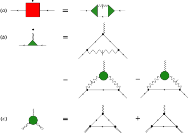
Figure 7: (Color online) (a) Graphical representation of the FRG flow equation (77) for the fermionic self-energy in the momentum-transfer cutoff scheme. This flow equation can be obtained from the more general flow equation (34) by omitting the contribution involving the fermionic single-scale propagator. (b) Truncated flow equation for the three-legged vertex $\Gamma^{\bar{\psi}^{\alpha}\psi^{\alpha}\phi}(K+\bar{K};K;\bar{K})$ in the momentum-transfer cutoff scheme, which can be obtained from the more general flow equation (42) shown in Fig. 4 by neglecting the contribution from the fermionic single-scale propagator and approximating the vertices $\Gamma^{\bar{\psi}^{\alpha}\psi^{\alpha}\phi}(K+\bar{K};K;\bar{K})$ on the right-hand side by the bare vertices. (c) Graphical representation of the approximate expression (79) for the bosonic three-legged vertex used in our calculation. Note that this expression can be obtained from the exact skeleton equation (A3) derived in Appendix A by neglecting the irreducible four-point vertex and then making the same approximations as in (b).

To obtain the corrections to the one-loop approximation, it is sufficient to approximate all propagators in Eqs. (77)–(79) by the one-loop results given in Sec. IV, i.e., we approximate on the right-hand sides

$$G^{\alpha}_{\Lambda}(K) = \frac{Z_{\Lambda}}{i\omega-Z_{\Lambda}\xi^{\alpha}_{\bm{k}}},$$ (80)

$${F}_{\Lambda}(\bar{K}) = \frac{\Theta(|\bar{k}_{\bot}|-\Lambda)}{r_{0}+c_{0}|\bar{k}_{\bot}|^{z_{b}-1}+\Theta(|\bar{k}_{\bot}|-\Lambda)b_{0}|\bar{\omega}|/|\bar{k}_{\bot}|},\hskip 19.91692pt$$ (81)

$$\dot{F}_{\Lambda}(\bar{K}) = -\frac{\delta(|\bar{k}_{\bot}|-\Lambda)}{r_{0}+c_{0}\Lambda^{z_{b}-1}+b_{0}|\bar{\omega}|/\Lambda}.$$ (82)

Here, $Z_{\Lambda}$ is the one-loop result for the flowing wave-function renormalization factor given in Eq. (66) and we have used the fact that $\tilde{Z}_{\Lambda}=1$ within the one-loop approximation. We thus arrive at a system of flow equations for the momentum- and frequency-dependent two-point and three-point functions. Having determined the right-hand side of the flow equation (77) for the self-energy, we can substitute the result into Eqs. (LABEL:eq:etaflow2) and (76) and obtain for the flowing anomalous dimension related to the frequency dependence of the self-energy

$${\eta}_{\Lambda} = {Z}_{\Lambda}\Lambda\lim_{K\rightarrow 0}\frac{\partial}{\partial(i\omega)}\int_{\bar{K}}\dot{F}_{\Lambda}(\bar{K})[G^{\alpha}_{\Lambda}(\bar{K}+K)-G^{\alpha}_{\Lambda}(\bar{K})]$$ (83)

$$\hskip 56.9055pt\times[\Gamma^{\bar{\psi}^{\alpha}\psi^{\alpha}\phi}_{\Lambda}(\bar{K};0;\bar{K})]^{2}$$

$$+ 2{Z}_{\Lambda}\Lambda\int_{\bar{K}}\dot{F}_{\Lambda}(\bar{K})G^{\alpha}_{\Lambda}(\bar{K})\Gamma^{\bar{\psi}^{\alpha}\psi^{\alpha}\phi}_{\Lambda}(\bar{K};0;\bar{K})$$

$$\hskip 28.45274pt\times\lim_{K\rightarrow 0}\frac{\partial\Gamma^{\bar{\psi}^{\alpha}\psi^{\alpha}\phi}_{\Lambda}(\bar{K}+K;K;\bar{K})}{\partial(i\omega)},$$

and for the corresponding anomalous dimension associated with the momentum dependence of the self-energy,

$$\tilde{\eta}_{\Lambda} = -\tilde{Z}_{\Lambda}\Lambda\lim_{K\rightarrow 0}\frac{\partial}{\partial(\alpha k_{\parallel})}\int_{\bar{K}}\dot{F}_{\Lambda}(\bar{K})[G^{\alpha}_{\Lambda}(\bar{K}+K)-G^{\alpha}_{\Lambda}(\bar{K})]$$ (84)

$$\hskip 56.9055pt\times[\Gamma^{\bar{\psi}^{\alpha}\psi^{\alpha}\phi}_{\Lambda}(\bar{K};0;\bar{K})]^{2}$$

$$- 2\tilde{Z}_{\Lambda}\Lambda\int_{\bar{K}}\dot{F}_{\Lambda}(\bar{K})G^{\alpha}_{\Lambda}(\bar{K})\Gamma^{\bar{\psi}^{\alpha}\psi^{\alpha}\phi}_{\Lambda}(\bar{K};0;\bar{K})$$

$$\hskip 28.45274pt\times\lim_{K\rightarrow 0}\frac{\partial\Gamma^{\bar{\psi}^{\alpha}\psi^{\alpha}\phi}_{\Lambda}(\bar{K}+K;K;\bar{K})}{\partial(\alpha k_{\parallel})}.$$

In the first terms on the right-hand sides of these expressions we have used the same regularization as in Eq. (50).

V.2 Bosonic three-legged vertex

In order to evaluate the self-energy from Eq. (77), we should calculate the mixed fermion-boson vertex ${\Gamma}^{\bar{\psi}^{\alpha}\psi^{\alpha}\phi}(K+\bar{K};K;\bar{K})$ by integrating the flow equation (78), which in turn depends on the purely bosonic three-legged vertex $\Gamma^{\phi\phi\phi}(\bar{K}_{1},\bar{K}_{2},-\bar{K}_{1}-\bar{K}_{2})$. Fortunately, the integrations in the truncated skeleton equation (79) can be carried out exactly in our model, as shown in Appendix B. The result can be written as

$$\Gamma^{\phi\phi\phi}(\bar{K}_{1},\bar{K}_{2},-\bar{K}_{1}-\bar{K}_{2})$$ (85)

$$= 2!N\sum_{\alpha}(\Gamma_{0}^{\alpha})^{3}L^{\alpha}_{3}(\bar{K}_{1},\bar{K}_{2},-\bar{K}_{1}-\bar{K}_{2}),$$

where the symmetrized fermion loop with three external bosonic legs and one-loop renormalized fermionic propagators is given by

$$L^{\alpha}_{3}(\bar{K}_{1},\bar{K}_{2},-\bar{K}_{1}-\bar{K}_{2}) = \frac{1}{4\pi}\left(\frac{1}{\bar{k}_{\bot 1}}+\frac{1}{\bar{k}_{\bot 2}}\right)\frac{\bar{\omega}_{1}\Theta\left(\frac{\bar{\omega}_{1}}{\bar{k}_{\bot 1}}\right)+\bar{\omega}_{2}\Theta\left(\frac{\bar{\omega}_{2}}{\bar{k}_{\bot 2}}\right)-(\bar{\omega}_{1}+\bar{\omega}_{2})\Theta\left(\frac{\bar{\omega}_{1}+\bar{\omega}_{2}}{\bar{k}_{\bot 1}+\bar{k}_{\bot 2}}\right)}{\left[\frac{\bar{k}_{\parallel 1}}{\bar{k}_{\bot 1}}-\frac{\bar{k}_{\parallel 2}}{\bar{k}_{\bot 2}}-\frac{i\alpha}{Z}(\frac{\bar{\omega}_{1}}{\bar{k}_{\bot 1}}-\frac{\bar{\omega}_{2}}{\bar{k}_{\bot 2}})\right]^{2}-(\bar{k}_{\bot 1}+\bar{k}_{\bot 2})^{2}}.$$ (86)

Note that this function represents a rather complicated momentum- and frequency-dependent effective interaction between the bosonic fluctuations, mediated by the fermions. Obviously, this function cannot simply be approximated by a constant, which is assumed to be possible in the Hertz-Millis approach to quantum critical phenomena.Hertz (1976); Millis (1993)

V.3 Three-legged boson-fermion vertex

We have now calculated all functions appearing on the right-hand side of the FRG flow equation (78) for the three-legged vertex with one bosonic and two fermionic external legs, so that we may next integrate this equation over the flow parameter $\Lambda$. Let us begin by evaluating the first term on the right-hand side of Eq. (78),

$$\partial_{\Lambda}{\Gamma}^{\bar{\psi}^{\alpha}\psi^{\alpha}\phi}(K+\bar{K};K;\bar{K})^{(1)}=(\Gamma_{0}^{\alpha})^{3}\int_{\bar{K}^{\prime}}\dot{F}(\bar{K}^{\prime})$$

$$\times G^{\alpha}(K+\bar{K}^{\prime})G^{\alpha}(K+\bar{K}+\bar{K}^{\prime}),$$ (87)

corresponding to the first diagram on the right-hand side of Fig. 7 (b). The integrations in Eq. (87) can be explicitly carried out, with the result

$$\Lambda\partial_{\Lambda}{\Gamma}^{\bar{\psi}^{\alpha}\psi^{\alpha}\phi}(K+\bar{K};K;\bar{K})^{(1)} = -\frac{(\Gamma_{0}^{\alpha})^{3}}{(2\pi)^{2}}\frac{Z_{\Lambda}}{b_{0}}\left[\frac{\Lambda^{2}}{i\bar{\omega}-Z_{\Lambda}[\alpha\bar{k}_{\parallel}+\bar{k}_{\bot}^{2}+2\bar{k}_{\bot}(k_{\bot}+\Lambda)]}+(\Lambda\rightarrow-\Lambda)\right]$$ (88)

$$\times \left[i\,{\rm sgn}(\omega+\bar{\omega})\ln\left(1+\frac{b_{0}|\omega+\bar{\omega}|}{r_{0}\Lambda+c_{0}\Lambda^{z_{b}}}\right)-i\,{\rm sgn}(\omega)\ln\left(1+\frac{b_{0}|\omega|}{r_{0}\Lambda+c_{0}\Lambda^{z_{b}}}\right)\right].$$

For the evaluation of the flowing anomalous dimensions in Eqs. (83) and (84), we need only the vertex ${\Gamma}^{\bar{\psi}^{\alpha}\psi^{\alpha}\phi}(\bar{K};0;\bar{K})$ at vanishing fermionic energy-momentum, as well as the derivatives of ${\Gamma}^{\bar{\psi}^{\alpha}\psi^{\alpha}\phi}(\bar{K}+K;K;\bar{K})$ with respect to the components of $K$ at $K=0$. From Eq. (88), we see that the contribution of the first diagram in Fig. 7 (b) to the flow of these quantities can be written as

$$\Lambda\partial_{\Lambda}{\Gamma}^{\bar{\psi}^{\alpha}\psi^{\alpha}\phi}(\bar{K};0;\bar{K})^{(1)}=-I^{(1)}_{\Lambda}\left(\frac{\bar{\omega}}{\Lambda^{z_{b}}},\frac{\bar{k}_{\parallel}}{\Lambda^{2}},\frac{\bar{k}_{\bot}}{\Lambda}\right),\hskip 19.91692pt$$ (89)

$$\Lambda\partial_{\Lambda}\left.\frac{\partial{\Gamma}^{\bar{\psi}^{\alpha}\psi^{\alpha}\phi}(\bar{K};K;\bar{K})^{(1)}}{\partial(i\omega)}\right|_{K=0}$$

$$\hskip 56.9055pt=-\frac{1}{\Lambda^{z_{b}}}I^{(1\omega)}_{\Lambda}\left(\frac{\bar{\omega}}{\Lambda^{z_{b}}},\frac{\bar{k}_{\parallel}}{\Lambda^{2}},\frac{\bar{k}_{\bot}}{\Lambda}\right),$$ (90)

$$\Lambda\partial_{\Lambda}\left.\frac{\partial{\Gamma}^{\bar{\psi}^{\alpha}\psi^{\alpha}\phi}(\bar{K};K;\bar{K})^{(1)}}{\partial(\alpha k_{\parallel})}\right|_{K=0}=0,$$ (91)

where we have defined the dimensionless scaling functions

$$I^{(1)}_{\Lambda}(\bar{\epsilon},\bar{q}_{\parallel},\bar{q}_{\bot})=\frac{\gamma_{\Lambda}}{(2\pi)^{2}b_{0}}i\,{\rm sgn}(\bar{\epsilon})\ln\left(1+\frac{b_{0}|\bar{\epsilon}|}{r_{\Lambda}+c_{0}}\right)$$

$$\times\left[\frac{1}{i\bar{\epsilon}-\gamma_{\Lambda}[\alpha\bar{q}_{\parallel}+\bar{q}_{\bot}^{2}+2\bar{q}_{\bot}]}+(\bar{q}_{\bot}\rightarrow-\bar{q}_{\bot})\right],$$ (92)

and

$$I^{(1\omega)}_{\Lambda}(\bar{\epsilon},\bar{q}_{\parallel},\bar{q}_{\bot})=-\frac{\gamma_{\Lambda}}{(2\pi)^{2}(r_{\Lambda}+c_{0})^{2}}\frac{b_{0}}{1+\frac{b_{0}}{r_{\Lambda}+c_{0}}|\bar{\epsilon}|}$$

$$\times\left[\frac{|\bar{\epsilon}|}{i\bar{\epsilon}-\gamma_{\Lambda}[\alpha\bar{q}_{\parallel}+\bar{q}_{\bot}^{2}+2\bar{q}_{\bot}]}+(\bar{q}_{\bot}\rightarrow-\bar{q}_{\bot})\right].\hskip 19.91692pt$$ (93)

Here, $r_{\Lambda}=r_{0}\Lambda^{1-z_{b}}$ vanishes at the quantum critical point, and we have introduced the dimensionless parameter

$$\gamma_{\Lambda}=\frac{Z_{\Lambda}}{\Lambda^{z_{b}-2}}=\frac{2\pi^{2}c_{0}(z_{b}-2)}{1-\Lambda^{z_{b}-2}\bigl{[}\frac{2\pi^{2}c_{0}(z_{b}-2)}{Z_{\Lambda_{0}}}-\Lambda_{0}^{2-z_{b}}\bigr{]}},$$ (94)

which approaches the limit $2\pi^{2}c_{0}(z_{b}-2)\propto N(z_{b}-2)$ for $\Lambda\rightarrow 0$.

Next, consider the contribution of the last two diagrams on the right-hand side of Fig. 7 (b) to the flow of the three-legged boson-fermion vertex, corresponding to the second line in Eq. (78),

$$\partial_{\Lambda}{\Gamma}^{\bar{\psi}^{\alpha}\psi^{\alpha}\phi}(K+\bar{K};K;\bar{K})^{(2)} = -(\Gamma_{0}^{\alpha})^{2}\int_{\bar{K}^{\prime}}\dot{F}(\bar{K}^{\prime})F(\bar{K}+\bar{K}^{\prime})\left[G^{\alpha}(K+\bar{K}+\bar{K}^{\prime})+G^{\alpha}(K-\bar{K}^{\prime})\right]$$ (95)

$$\hskip 51.21495pt\times\Gamma^{\phi\phi\phi}(\bar{K},\bar{K}^{\prime},-\bar{K}-\bar{K}^{\prime}).$$

Due to the rather complicated form of the vertex $\Gamma^{\phi\phi\phi}(\bar{K},\bar{K}^{\prime},-\bar{K}-\bar{K}^{\prime})$ given in Eqs. (85) and (86), the evaluation of the right-hand side of Eq. (95) is quite involved. The $\bar{k}_{\parallel}^{\prime}$ integration can still be performed by means of the residue theorem, while the $\bar{k}_{\bot}^{\prime}$ integration is trivial due to the $\delta$-function in the single-scale propagator. After these integrations, we obtain

$$\partial_{\Lambda}{\Gamma}^{\bar{\psi}^{\alpha}\psi^{\alpha}\phi}(K+\bar{K};K;\bar{K})^{(2)}=-i\alpha N\Lambda^{2}\frac{(\Gamma_{0}^{\alpha})^{2}}{(2\pi)^{2}}\int_{-\infty}^{\infty}\frac{d\bar{\omega}^{\prime}}{2\pi}\frac{1}{r_{0}+c_{0}\Lambda^{z_{b}-1}+b_{0}|\bar{\omega}^{\prime}|/\Lambda}$$ (96)

$$\times \sum_{s=\pm}F(\bar{\omega}+\bar{\omega}^{\prime},\bar{k}_{\bot}+s\Lambda)J(\bar{\omega},\bar{k}_{\bot},\bar{\omega}^{\prime},s\Lambda)\sum_{\alpha^{\prime}=\pm}(\Gamma_{0}^{\alpha^{\prime}})^{3}\left[\frac{\Theta({\rm Im}(z_{1}))-\Theta({\rm Im}(z_{3}))}{(z_{1}-z_{3})^{2}-z_{4}^{2}}-\frac{\Theta({\rm Im}(z_{2}))-\Theta({\rm Im}(z_{3}))}{(z_{2}-z_{3})^{2}-z_{4}^{2}}\right],\hskip 14.22636pt$$

where

$$J(\bar{\omega},\bar{k}_{\bot},\bar{\omega}^{\prime},\bar{k}_{\bot}^{\prime})=\left(\frac{1}{\bar{k}_{\bot}}+\frac{1}{\bar{k}_{\bot}^{\prime}}\right)\left[\bar{\omega}\Theta\left(\frac{\bar{\omega}}{\bar{k}_{\bot}}\right)+\bar{\omega}^{\prime}\Theta\left(\frac{\bar{\omega}^{\prime}}{\bar{k}_{\bot}^{\prime}}\right)-(\bar{\omega}+\bar{\omega}^{\prime})\Theta\left(\frac{\bar{\omega}+\bar{\omega}^{\prime}}{\bar{k}_{\bot}+\bar{k}_{\bot}^{\prime}}\right)\right],$$ (97)

and

$$z_{1} = -(k_{\parallel}+\bar{k}_{\parallel})-\alpha[\Lambda+s(k_{\bot}+\bar{k}_{\bot})]^{2}$$ (98a)

$$+\frac{i\bar{\omega}^{\prime}+i\bar{\omega}+i\omega}{Z_{\Lambda}},$$

$$z_{2} = k_{\parallel}+\alpha(\Lambda-sk_{\bot})^{2}+\alpha\frac{i\bar{\omega}^{\prime}-i\omega}{Z_{\Lambda}},$$ (98b)

$$z_{3} = \Lambda\left[\frac{\bar{k}_{\parallel}}{s\bar{k}_{\bot}}-\frac{\alpha^{\prime}}{Z_{\Lambda}}\left(\frac{i\bar{\omega}}{s\bar{k}_{\bot}}-\frac{i\bar{\omega}^{\prime}}{\Lambda}\right)\right],$$ (98c)

$$z_{4} = \Lambda(\Lambda+s\bar{k}_{\bot}).$$ (98d)

For the calculation of $\eta_{\Lambda}$ and $\tilde{\eta}_{\Lambda}$ in Eqs. (83) and (84) we, again, need only the vertex ${\Gamma}^{\bar{\psi}^{\alpha}\psi^{\alpha}\phi}(\bar{K};0;\bar{K})$ and the derivatives of ${\Gamma}^{\bar{\psi}^{\alpha}\psi^{\alpha}\phi}(\bar{K}+K;K;\bar{K})$ with respect to the components of the fermionic label $K$ at $K=0$. In analogy with Eqs. (89)–(91), we therefore define

$$\Lambda\partial_{\Lambda}{\Gamma}^{\bar{\psi}^{\alpha}\psi^{\alpha}\phi}(\bar{K};0;\bar{K})^{(2)}=-I^{(2)}_{\Lambda}\left(\frac{\bar{\omega}}{\Lambda^{z_{b}}},\frac{\bar{k}_{\parallel}}{\Lambda^{2}},\frac{\bar{k}_{\bot}}{\Lambda}\right),\hskip 19.91692pt$$ (99)

$$\Lambda\partial_{\Lambda}\left.\frac{\partial{\Gamma}^{\bar{\psi}^{\alpha}\psi^{\alpha}\phi}(\bar{K};K;\bar{K})^{(2)}}{\partial(i\omega)}\right|_{K=0}$$

$$\hskip 56.9055pt=-\frac{1}{\Lambda^{z_{b}}}I^{(2\omega)}_{\Lambda}\left(\frac{\bar{\omega}}{\Lambda^{z_{b}}},\frac{\bar{k}_{\parallel}}{\Lambda^{2}},\frac{\bar{k}_{\bot}}{\Lambda}\right),$$ (100)

$$\Lambda\partial_{\Lambda}\left.\frac{\partial{\Gamma}^{\bar{\psi}^{\alpha}\psi^{\alpha}\phi}(\bar{K};K;\bar{K})^{(2)}}{\partial(\alpha k_{\parallel})}\right|_{K=0}$$

$$\hskip 56.9055pt=-\frac{1}{\Lambda^{2}}I^{(2k)}_{\Lambda}\left(\frac{\bar{\omega}}{\Lambda^{z_{b}}},\frac{\bar{k}_{\parallel}}{\Lambda^{2}},\frac{\bar{k}_{\bot}}{\Lambda}\right).$$ (101)

From now on we focus on the Ising-nematic instability and explicitly set $\Gamma_{0}^{\alpha}=1$. In principle, the functions $I^{(2)}_{\Lambda}(\bar{\epsilon},\bar{q}_{\parallel},\bar{q}_{\bot})$, $I^{(2\omega)}_{\Lambda}(\bar{\epsilon},\bar{q}_{\parallel},\bar{q}_{\bot})$, and $I^{(2k)}_{\Lambda}(\bar{\epsilon},\bar{q}_{\parallel},\bar{q}_{\bot})$ can be calculated analytically by performing the remaining frequency integration in Eq. (96). However, the result is rather cumbersome and not very transparent. To simplify the calculation, let us assume that the arguments $\bar{\epsilon}$, $\bar{q}_{\parallel}$, and $\bar{q}_{\bot}$ of these functions are all small compared with unity. Then the resulting expressions simplify and we obtain the approximate expressions

$$I^{(2)}_{\Lambda}(\bar{\epsilon},\bar{q}_{\parallel},\bar{q}_{\bot}) \approx \frac{\gamma_{\Lambda}|\bar{\epsilon}|N}{2(2\pi)^{3}(r_{\Lambda}+c_{0})^{2}}\biggl{[}\frac{1}{|\bar{q}_{\bot}|-w}$$ (102)

$$-\frac{|\bar{q}_{\bot}|}{(|\bar{q}_{\bot}|-w)^{2}}\ln\left(\frac{|\bar{q}_{\bot}|}{w}\right)\biggr{]},$$

$$I^{(2\omega)}_{\Lambda}(\bar{\epsilon},\bar{q}_{\parallel},\bar{q}_{\bot}) \approx \frac{\gamma_{\Lambda}N}{(2\pi)^{3}(r_{\Lambda}+c_{0})^{2}}\Biggl{[}\frac{\alpha\gamma_{\Lambda}\bar{q}_{\parallel}|\bar{\epsilon}|}{\bar{\epsilon}^{2}+\gamma_{\Lambda}^{2}\bar{q}_{\parallel}^{2}}$$ (103)

$$-i\,{\rm sgn}(\bar{\epsilon})|\bar{q}_{\bot}|\frac{\bar{\epsilon}^{2}(\bar{\epsilon}^{2}-\gamma_{\Lambda}^{2}\bar{q}_{\parallel}^{2})}{(\bar{\epsilon}^{2}+\gamma_{\Lambda}^{2}\bar{q}_{\parallel}^{2})^{2}}\Biggr{]},\hskip 19.91692pt$$

$$I^{(2k)}_{\Lambda}(\bar{\epsilon},\bar{q}_{\parallel},\bar{q}_{\bot}) \approx \frac{i\,{\rm sgn}(\bar{\epsilon})\gamma_{\Lambda}^{2}|\bar{q}_{\bot}|N}{(2\pi)^{3}(r_{\Lambda}+c_{0})^{2}}\frac{\bar{\epsilon}^{2}(\bar{\epsilon}^{2}-\gamma_{\Lambda}^{2}\bar{q}_{\parallel}^{2})}{(\bar{\epsilon}^{2}+\gamma_{\Lambda}^{2}\bar{q}_{\parallel}^{2})^{2}},\hskip 19.91692pt$$ (104)

where, in Eq. (102), the complex quantity $w$ is defined by

$$w=\frac{b_{0}}{2(r_{\Lambda}+c_{0})}\left(|\bar{\epsilon}|-i\alpha\gamma_{\Lambda}\bar{q}_{\parallel}{\rm sgn}(\bar{\epsilon})\right).$$ (105)

Let us now combine the contributions from all three diagrams on the right-hand side of Fig. 7 (b). To be consistent with the approximations made in the derivation of Eqs. (102)–(104), we should also expand the right-hand sides of $I^{(1)}_{\Lambda}(\bar{\epsilon},\bar{q}_{\parallel},\bar{q}_{\bot})$ and $I^{(1\omega)}_{\Lambda}(\bar{\epsilon},\bar{q}_{\parallel},\bar{q}_{\bot})$ in Eqs. (92) and (93) for small $\bar{\epsilon}$. We therefore define

$$I_{\Lambda}(\bar{\epsilon},\bar{q}_{\parallel},\bar{q}_{\bot}) = I^{(1)}_{\Lambda}(\bar{\epsilon},\bar{q}_{\parallel},\bar{q}_{\bot})+I^{(2)}_{\Lambda}(\bar{\epsilon},\bar{q}_{\parallel},\bar{q}_{\bot})$$ (106a)

$$= \frac{\gamma_{\Lambda}}{(2\pi)^{2}(r_{\Lambda}+c_{0})}\Biggl{\{}\frac{i\bar{\epsilon}}{i\bar{\epsilon}-\gamma_{\Lambda}[\alpha\bar{q}_{\parallel}+\bar{q}_{\bot}^{2}+2\bar{q}_{\bot}]}+\frac{i\bar{\epsilon}}{i\bar{\epsilon}-\gamma_{\Lambda}[\alpha\bar{q}_{\parallel}+\bar{q}_{\bot}^{2}-2\bar{q}_{\bot}]}$$

$$\hskip 65.44133pt+\frac{N}{4\pi(r_{\Lambda}+c_{0})}\Biggl{[}\frac{|\bar{\epsilon}|}{|\bar{q}_{\bot}|-w}-\frac{|\bar{q}_{\bot}||\bar{\epsilon}|}{(|\bar{q}_{\bot}|-w)^{2}}\ln\left(\frac{|\bar{q}_{\bot}|}{w}\right)\Biggr{]}\Biggr{\}},\hskip 19.91692pt$$

$$I^{(\omega)}_{\Lambda}(\bar{\epsilon},\bar{q}_{\parallel},\bar{q}_{\bot}) = I^{(1\omega)}_{\Lambda}(\bar{\epsilon},\bar{q}_{\parallel},\bar{q}_{\bot})+I^{(2\omega)}_{\Lambda}(\bar{\epsilon},\bar{q}_{\parallel},\bar{q}_{\bot})$$ (106b)

$$= \frac{\gamma_{\Lambda}b_{\Lambda}}{(2\pi)^{2}(r_{\Lambda}+c_{0})^{2}}\Biggl{\{}-\frac{|\bar{\epsilon}|}{i\bar{\epsilon}-\gamma_{\Lambda}[\alpha\bar{q}_{\parallel}+\bar{q}_{\bot}^{2}+2\bar{q}_{\bot}]}-\frac{|\bar{\epsilon}|}{i\bar{\epsilon}-\gamma_{\Lambda}[\alpha\bar{q}_{\parallel}+\bar{q}_{\bot}^{2}-2\bar{q}_{\bot}]}$$

$$\hskip 65.44133pt+\frac{N}{2\pi b_{\Lambda}}\Biggl{[}\frac{\alpha\gamma_{\Lambda}\bar{q}_{\parallel}|\bar{\epsilon}|}{\bar{\epsilon}^{2}+\gamma_{\Lambda}^{2}\bar{q}_{\parallel}^{2}}-|\bar{q}_{\bot}|\frac{i\bar{\epsilon}|\bar{\epsilon}|(\bar{\epsilon}^{2}-\gamma_{\Lambda}^{2}\bar{q}_{\parallel}^{2})}{(\bar{\epsilon}^{2}+\gamma_{\Lambda}^{2}\bar{q}_{\parallel}^{2})^{2}}\Biggr{]}\Biggr{\}},$$

$$I^{(k)}_{\Lambda}(\bar{\epsilon},\bar{q}_{\parallel},\bar{q}_{\bot}) = I^{(2k)}_{\Lambda}(\bar{\epsilon},\bar{q}_{\parallel},\bar{q}_{\bot})=\frac{\gamma_{\Lambda}^{2}|\bar{q}_{\bot}|N}{(2\pi)^{3}(r_{\Lambda}+c_{0})^{2}}\frac{i\bar{\epsilon}|\bar{\epsilon}|(\bar{\epsilon}^{2}-\gamma_{\Lambda}^{2}\bar{q}_{\parallel}^{2})}{(\bar{\epsilon}^{2}+\gamma_{\Lambda}^{2}\bar{q}_{\parallel}^{2})^{2}}.$$ (106c)

Finally, we integrate over the flow parameter $\Lambda$, and obtain the following expressions for the three-legged boson-fermion vertex,

$${\Gamma}^{\bar{\psi}^{\alpha}\psi^{\alpha}\phi}(\bar{K};0;\bar{K}) = \tilde{\Gamma}_{\Lambda}(\bar{\epsilon},\bar{q}_{\parallel},\bar{q}_{\bot}),$$ (107a)

$$\left.\frac{\partial{\Gamma}^{\bar{\psi}^{\alpha}\psi^{\alpha}\phi}(\bar{K};K;\bar{K})}{\partial(i\omega)}\right|_{K=0} = \frac{1}{\Lambda^{z_{b}}}\tilde{\Gamma}^{\omega}_{\Lambda}(\bar{\epsilon},\bar{q}_{\parallel},\bar{q}_{\bot}),\hskip 19.91692pt$$ (107b)

$$\left.\frac{\partial{\Gamma}^{\bar{\psi}^{\alpha}\psi^{\alpha}\phi}(\bar{K};K;\bar{K})}{\partial(\alpha k_{\parallel})}\right|_{K=0} = \frac{1}{\Lambda^{2}}\tilde{\Gamma}^{k}_{\Lambda}(\bar{\epsilon},\bar{q}_{\parallel},\bar{q}_{\bot}),$$ (107c)

where

$$\tilde{\Gamma}_{\Lambda}(\bar{\epsilon},\bar{q}_{\parallel},\bar{q}_{\bot})=1+\int_{\Lambda/\Lambda_{0}}^{1}\frac{ds}{s}I_{\Lambda/s}\left(s^{z_{b}}\bar{\epsilon},s^{2}\bar{q}_{\parallel},s\bar{q}_{\bot}\right),\hskip 19.91692pt$$

(108a)

$$\tilde{\Gamma}^{\omega}_{\Lambda}(\bar{\epsilon},\bar{q}_{\parallel},\bar{q}_{\bot})=\int_{\Lambda/\Lambda_{0}}^{1}ds\,s^{z_{b}-1}I^{\omega}_{\Lambda/s}\left(s^{z_{b}}\bar{\epsilon},s^{2}\bar{q}_{\parallel},s\bar{q}_{\bot}\right),$$

(108b)

$$\tilde{\Gamma}^{k}_{\Lambda}(\bar{\epsilon},\bar{q}_{\parallel},\bar{q}_{\bot})=\int_{\Lambda/\Lambda_{0}}^{1}ds\,sI^{k}_{\Lambda/s}\left(s^{z_{b}}\bar{\epsilon},s^{2}\bar{q}_{\parallel},s\bar{q}_{\bot}\right).$$ (108c)

Recall that in deriving these expressions we have assumed that $|\bar{\epsilon}|\lesssim 1$.

V.4 Fermionic anomalous dimension and dynamic exponent

We are now ready to calculate the anomalous dimensions $\eta=\lim_{\Lambda\rightarrow 0}\eta_{\Lambda}$ and $\tilde{\eta}=\lim_{\Lambda\rightarrow 0}\tilde{\eta}_{\Lambda}$ at the quantum critical point. We therefore substitute Eqs. (107a)– (107c) into our general relations (83) and (84) for the flowing anomalous dimensions ${\eta}_{\Lambda}$ and $\tilde{\eta}_{\Lambda}$ and, introducing the integration variables $p=\gamma_{\Lambda}\alpha\bar{q}_{\parallel}$ and $y=\bar{\epsilon}$, we obtain for the flowing anomalous dimension associated with the frequency dependence of the self-energy,

$$\eta_{\Lambda} = -\frac{\gamma_{\Lambda}}{2\pi}\lim_{\omega\rightarrow 0}\frac{\partial}{\partial(i\omega)}\int_{-\lambda_{0}}^{\lambda_{0}}\frac{dy}{2\pi}\int_{-\infty}^{\infty}\frac{dp}{2\pi}\left[\frac{1}{r_{\Lambda}+c_{0}+b_{0}|y|}\right]\left[\frac{1}{iy+i\omega-p-\gamma_{\Lambda}}-\frac{1}{iy-p-\gamma_{\Lambda}}\right]\left[\tilde{\Gamma}_{\Lambda}\left(y,\frac{p}{\alpha\gamma_{\Lambda}},1\right)\right]^{2}$$ (109)

$$-\frac{\gamma_{\Lambda}}{\pi}\int_{-\lambda_{0}}^{\lambda_{0}}\frac{dy}{2\pi}\int_{-\infty}^{\infty}\frac{dp}{2\pi}\left[\frac{1}{r_{\Lambda}+c_{0}+b_{0}|y|}\right]\left[\frac{1}{iy-p-\gamma_{\Lambda}}\right]\tilde{\Gamma}_{\Lambda}\left(y,\frac{p}{\alpha\gamma_{\Lambda}},1\right)\tilde{\Gamma}^{\omega}_{\Lambda}\left(y,\frac{p}{\alpha\gamma_{\Lambda}},1\right),$$

and for the corresponding anomalous dimension associated with the momentum dependence of the self-energy,

$$\tilde{\eta}_{\Lambda} = \frac{\gamma_{\Lambda}}{2\pi}\lim_{k\rightarrow 0}\frac{\partial}{\partial k}\int_{-\lambda_{0}}^{\lambda_{0}}\frac{dy}{2\pi}\int_{-\infty}^{\infty}\frac{dp}{2\pi}\left[\frac{1}{r_{\Lambda}+c_{0}+b_{0}|y|}\right]\left[\frac{1}{iy-p-k-\gamma_{\Lambda}}-\frac{1}{iy-p-\gamma_{\Lambda}}\right]\left[\tilde{\Gamma}_{\Lambda}\left(y,\frac{p}{\alpha\gamma_{\Lambda}},1\right)\right]^{2}$$ (110)

$$+\frac{1}{\pi}\int_{-\lambda_{0}}^{\lambda_{0}}\frac{dy}{2\pi}\int_{-\infty}^{\infty}\frac{dp}{2\pi}\left[\frac{1}{r_{\Lambda}+c_{0}+b_{0}|y|}\right]\left[\frac{1}{iy-p-\gamma_{\Lambda}}\right]\tilde{\Gamma}_{\Lambda}\left(y,\frac{p}{\alpha\gamma_{\Lambda}},1\right)\tilde{\Gamma}^{k}_{\Lambda}\left(y,\frac{p}{\alpha\gamma_{\Lambda}},1\right).$$

Here, $\lambda_{0}$ is an ultraviolet cutoff of the order of unity which takes into account that our expressions (106a)–(106c) which we use to calculate the vertices in Eqs. (108a)–(108c) are only valid for small frequencies.

Consider now the limit $\Lambda\rightarrow 0$. At the quantum critical point we may then set $r_{\Lambda}\rightarrow 0$. For simplicity, we also set $c_{0}=b_{0}=N/(4\pi)$. To make progress analytically, let us further assume that the parameter $\gamma=\lim_{\Lambda\rightarrow 0}\gamma_{\Lambda}=2\pi^{2}c_{0}(z_{b}-2)=\frac{\pi}{2}N(z_{b}-2)$ is small compared with unity. To leading order in $z_{b}-2$ the $s$-integrations in Eqs. (108a)– (108c) can then be carried out analytically, with the result

$$\lim_{\Lambda\rightarrow 0}\tilde{\Gamma}_{\Lambda}\left(y,\frac{p}{\alpha\gamma_{\Lambda}},1\right) = 1+\frac{\gamma}{(2\pi)^{2}c_{0}}\biggl{\{}\frac{iy}{iy-p-\gamma}\ln\Bigl{[}1-\Bigl{(}\frac{iy-p-\gamma}{2\gamma}\Bigr{)}^{2}\Bigr{]}$$ (111)

$$\hskip 56.9055pt-\frac{iyN}{2\pi c_{0}}\biggl{[}\frac{\ln\bigl{[}\frac{2i\,{\rm sgn}(y)}{iy+p}\bigr{]}}{2i\,{\rm sgn}(y)-(iy+p)}+2\frac{\ln\bigl{[}1-\frac{iy+p}{2i\,{\rm sgn}(y)}\bigr{]}}{iy+p}\biggr{]}\biggr{\}},\hskip 19.91692pt$$

$$\lim_{\Lambda\rightarrow 0}\tilde{\Gamma}^{\omega}_{\Lambda}\left(y,\frac{p}{\alpha\gamma_{\Lambda}},1\right) = \frac{\gamma}{(2\pi)^{2}c_{0}}\biggl{\{}-\frac{|y|}{iy-p}+\frac{N}{2\pi c_{0}}\biggl{[}\frac{|y|p}{y^{2}+p^{2}}-\frac{iy|y|(y^{2}-p^{2})}{3(y^{2}+p^{2})^{2}}\biggr{]}\biggr{\}},$$ (112)

$$\lim_{\Lambda\rightarrow 0}\tilde{\Gamma}^{k}_{\Lambda}\left(y,\frac{p}{\alpha\gamma_{\Lambda}},1\right) = \frac{\gamma^{2}N}{(2\pi)^{3}c_{0}^{2}}\frac{iy|y|(y^{2}-p^{2})}{3(y^{2}+p^{2})^{2}}.$$ (113)

Note that these vertex functions describe the renormalized effective interaction between two fermions and one boson; clearly, this interaction has a rather complicated dependence on momenta and frequencies and cannot be approximated by a constant. If we now substitute Eqs. (111)–(113) into Eqs. (109) and (110), we may perform the $p$-integration analytically by means of the method of residues. Note that the first term in the curly braces of Eq. (111) and the first term in the curly braces of Eq. (112) do not contribute to the integrals, because we may close the integration contour in a half plane where the integrand is analytic. These terms arise from the first diagram on the right-hand side of Fig. 7 (b), so that the three-boson vertex is crucial to obtain the leading corrections to the anomalous dimensions. We finally arrive at the following estimates for the anomalous dimensions at the nematic quantum critical point,

$$\eta = z_{b}-2+\frac{(z_{b}-2)^{2}}{2}C(\lambda_{0})+{\cal{O}}((z_{b}-2)^{3}),$$ (114)

$$\tilde{\eta} = \frac{(z_{b}-2)^{2}}{2}\tilde{C}(\lambda_{0})+{\cal{O}}((z_{b}-2)^{3}),$$ (115)

where the cutoff functions are given by

$$C(\lambda_{0}) = \int_{0}^{\lambda_{0}}\frac{dy}{1+y}\left[\frac{7}{6}+\frac{1}{1-y}+\frac{y\ln y}{(1-y)^{2}}\right],$$ (116)

$$\tilde{C}(\lambda_{0}) = \int_{0}^{\lambda_{0}}\frac{dy}{1+y}\left[\frac{1}{6}+\frac{1}{1-y}+\frac{y\ln y}{(1-y)^{2}}\right]$$ (117)

$$= C(\lambda_{0})-\ln(1+\lambda_{0}).$$

A plot of the cutoff functions is shown in Fig. 8.

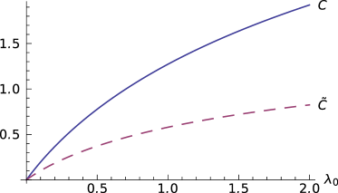
Figure 8: (Color online) Plot of the cutoff functions $C(\lambda_{0})$ and $\tilde{C}(\lambda_{0})$ defined in Eqs. (116) and (117).

Note that these functions depend logarithmically on the ultraviolet cutoff, $\lambda_{0}$. This is due to the fact that we have assumed that the rescaled frequencies and momenta in Eqs. (102)–(104) are small compared with unity in the evaluation of the vertex-correction diagrams shown in Fig. 7 (b). By retaining the full momentum- and frequency dependence on the right-hand side of the flow equation (96), one obtains ultraviolet convergent results from our FRG approach. However, as the cutoff dependence in our final result, Eqs. (114) and (115), is only logarithmic, we have not attempted to carry out this calculation which requires substantial numerical effort. Instead, we make the reasonable cutoff choice $\lambda_{0}=1$ and find, within the accuracy of our calculation, that $C\approx 1.27$ and $\tilde{C}\approx 0.58$.

Given our result for the anomalous dimensions $\eta$ and $\tilde{\eta}$, we may relate these to the anomalous dimension $\eta_{\psi}$ of the fermion field and the fermionic dynamic exponent, $z$. Let us therefore recall that, at the quantum critical point, the retarded single-particle Green function assumes for small frequencies and momenta the following scaling form,

$$G^{\alpha}(\omega+i0^{+},\bm{k})\propto\frac{1}{\left[A_{\omega}\,\text{sgn}({\omega})|\omega|^{1/z}-\xi_{\bm{k}}^{\alpha}\right]^{1-\eta_{\psi}/2}},$$ (118)

where $A_{\omega}$ is some dimensionful constant with positive imaginary part and real part depending on the sign of $\omega$, see Eq. (2). For $\omega=k_{\bot}=0$, this implies

$$G^{\alpha}(i0^{+},k_{\parallel},0)\propto k_{\parallel}^{-1+\eta_{\psi}/2}.$$ (119)

On the other hand, from the definition of $\tilde{\eta}_{\Lambda}$ in Eq. (62) we see that $\tilde{Z}_{\Lambda}\propto\Lambda^{\tilde{\eta}}\propto k_{\parallel}^{\tilde{\eta}/2}$, where we have used the fact that $k_{\parallel}$ scales as $\Lambda^{2}$. Hence,

$$G^{\alpha}(i0^{+},k_{\parallel},0)\propto\tilde{Z}_{\Lambda}/k_{\parallel}\propto k_{\parallel}^{-1+\tilde{\eta}/2}.$$ (120)

Comparing this with Eq. (119), we conclude that

$$\eta_{\psi}=\tilde{\eta}.$$ (121)

Next, setting $\bm{k}=0$ in Eq. (118), we find

$$G^{\alpha}(\omega+i0^{+},0)\propto\omega^{-(1-\eta_{\psi}/2)/z}.$$ (122)

On the other hand, from the definition of ${\eta}_{\Lambda}$ in Eq. (62) we infer that ${Z}_{\Lambda}\propto\Lambda^{{\eta}}\propto\omega^{{\eta}/(2z)}$ (using the fact that $\omega$ scales as $\Lambda^{2z}$), so that

$$G^{\alpha}(0,\omega+i0^{+})\propto Z_{\Lambda}/\omega\propto\omega^{-(1-\eta/(2z))}.$$ (123)

Comparing this with Eq. (122), we see that $1-\eta/(2z)=(1-\eta_{\psi}/2)/z$, or

$$z=1+\frac{\eta-\tilde{\eta}}{2}.$$ (124)

Writing Eq. (114) as $\eta=z_{b}-2+\delta\eta$ with

$$\delta\eta=\frac{(z_{b}-2)^{2}}{2}C(\lambda_{0})+{\cal{O}}((z_{b}-2)^{3}),$$ (125)

we see that Eq. (124) can also be written as

$$z = \frac{z_{b}}{2}+\frac{\delta\eta-\tilde{\eta}}{2}$$

$$= \frac{z_{b}}{2}+\frac{(z_{b}-2)^{2}}{4}\Bigl{[}{C}(\lambda_{0})-\tilde{C}(\lambda_{0})\Bigr{]}+{\cal{O}}((z_{b}-2)^{3}).$$

According to the above calculation, the scaling relation $z=z_{b}/2$ for the fermionic dynamic exponent acquires a correction of order $(z_{b}-2)^{2}$, such that the effective theory appears to have two different time scales. However, according to Metlitski and Sachdev,Metlitski and Sachdev (2010a) the strong correlations imply that $z=z_{b}/2$ should be satisfied exactly. This discrepancy might be due to the fact that our truncation of the FRG flow equations introduces approximations which violate the general scaling theory. In fact, this seems to be true also in the case of the loop expansion. In the previous works of Metlitski and SachdevMetlitski and Sachdev (2010a) and Mross et al.,Mross et al. (2010) the three-loop correction to the fermionic anomalous dimension $\eta_{\psi}$ is calculated via the momentum dependence of the self-energy, and according to scaling theory it is argued that a corresponding correction should appear if one calculates $\eta_{\psi}$ via the frequency dependence of the self-energy. However, as pointed out in Ref. Chubukov, 2010, the correction in the frequency dependence of the self-energy (the term $\delta\eta$ in our notation) appears only beyond the three-loop order. The FRG is not based on an expansion in powers of loops, so that diagrams beyond three loops are included in our truncation.

VI Summary and conclusions

In this work, we have used a functional renormalization group approach to calculate the anomalous dimension $\eta_{\psi}$ of the fermion field and the fermionic dynamic exponent $z$ of an effective low-energy field theory describing the Ising-nematic quantum critical point in two-dimensional metals. In the limit $N(z_{b}-2)\ll 1$ (where $N$ is the number of fermion flavors and $z_{b}$ is the bosonic dynamic exponent), we have been able to explicitly calculate the fermionic anomalous dimension $\eta_{\psi}$ of the system, with the result

$${\eta}_{\psi}\approx 0.3\left(z_{b}-2\right)^{2}+{\cal{O}}((z_{b}-2)^{3}).$$ (127)

If we extrapolate this expression to the physically relevant case, $z_{b}=3$, we obtain $\eta_{\psi}\approx 0.3$, which is larger than the estimate $\eta_{\psi}\approx 0.068$ given by Metlitski and Sachdev,Metlitski and Sachdev (2010a) but still smaller than the estimate $\eta_{\psi}\approx 0.6$ obtained from an extrapolation of the corresponding expression given by Mross et al..Mross et al. (2010) Given the different types of approximations, it is not surprising that different values for the exponent $\eta_{\psi}$ are found. This fact shows that the recent calculations done so far are not yet fully under control in the physically relevant case of $z_{b}=3$ and $N=2$. It is however reassuring that our method also finds a finite value for $\eta_{\psi}$. In particular, we note that in the previous calculations based on the field-theoretical renormalization group, the values of the exponent $\eta_{\psi}$ are obtained within a loop-expansion truncated at the three-loop order, while in our FRG approach the truncation does not rely on a loop-expansion, so that a certain class of diagrams beyond the three-loop level are effectively re-summed to higher order within our truncation. On the other hand, at the lowest order, namely at the one-loop level in the field theoretical RG and neglecting the vertex corrections in the FRG, the results obtained using the FRG and other renormalization group methods all coincide with the well-known results obtained within the RPA. Finally, in contrast to previous works,Metlitski and Sachdev (2010a); Mross et al. (2010) we have explicitly shown that both the frequency and the momentum dependence of the self-energy give rise to anomalous corrections to the one-loop result. While our calculations in principle lead to a small correction term to the fermionic dynamic critical exponent, $z$, the scaling theory of Metlitski and SachdevMetlitski and Sachdev (2010a) implies the exact identity $z=z_{b}/2$.

The calculations presented in this work can be extended in several directions. Because our FRG approach does not rely on the smallness of the parameter $N(z_{b}-2)$, with some numerical effort it should be possible to extract the anomalous dimension $\eta_{\psi}$ for general $N$ and $z_{b}-2$ from Eqs. (109) and (110). In this case the vertices appearing in these expressions cannot be calculated analytically but must be represented as one-dimensional integrals, so that the evaluation of the anomalous dimensions in Eqs. (109) and (110) requires rather complicated numerical integrations, which is beyond the scope of this work. In principle our FRG flow equations also allow us to calculate the entire frequency-dependence of the self-energies, but this seems to be numerically even more expensive.

In contrast to the strategy adopted in the Hertz-Millis approach,Hertz (1976); Millis (1993) in the present problem it is not possible to integrate over the fermionic degrees of freedom to obtain an effective bosonic theory with regular vertices. We have therefore explicitly retained both bosonic and fermionic degrees of freedom in our FRG calculation. The FRG approach developed in this work should also be useful to discuss other model systems where gapless fermionic and bosonic excitations are strongly coupled.

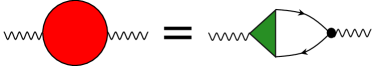
Figure 9: (Color online) Exact skeleton equation relating the bosonic self-energy to the exact fermionic propagators and the three-legged vertex with two fermion and one boson leg, see Eq. (A1). The black dot denotes the bare vertex with two fermionic and one bosonic external leg given in Eq. (11).

Appendix A: Skeleton equations

In sections IV and V, we have combined FRG flow equations with skeleton equations for the bosonic self-energy and the bosonic three-legged vertex to obtain a closed system of equations. In this appendix, we briefly describe the derivation of these skeleton equations.

Skeleton equations relating vertex functions of different order follow from the general Dyson-Schwinger equation for the generating functional for the connected Green function, which is a simple consequence of the invariance of the integration measure of the functional integral under infinitesimal shifts. The derivation of the skeleton equation for the bosonic self-energy of models of the type considered in this work has been discussed in detail in Refs. Bartosch et al., 2009a; Kopietz et al., 2010, so let us here only quote the result,

$${\Pi}(\bar{K})=\int_{K}\sum_{\alpha,\sigma}{G}^{\alpha}(K)G^{\alpha}(K+\bar{K})$$

$$\qquad\qquad{}\times\Gamma_{0}^{\alpha}\Gamma^{\bar{\psi}^{\alpha}\psi^{\alpha}\phi}(K;K+\bar{K};-\bar{K}).$$ (A1)

This exact identity is shown diagrammatically in Fig. 9.

To derive the skeleton equation for the three-boson vertex, let us start from the Dyson-Schwinger equation given in Eq. (11.27a) of Ref. Kopietz et al., 2010. After taking two successive derivatives with respect to $\phi_{{\bar{K}}_{2}}$ and $\phi_{{\bar{K}}_{3}}$, we obtain

$$\frac{\delta^{3}\Gamma}{\delta\phi_{{\bar{K}}_{1}}\,\delta\phi_{{\bar{K}}_{2}}\,\delta\phi_{{\bar{K}}_{3}}}=\sum_{\alpha,\sigma}\Gamma_{0}^{\alpha}\int_{{K}}\frac{\delta^{4}{\mathcal{G}}_{c}}{\delta\bar{\jmath}_{K}^{\alpha}\delta j_{K+\bar{K}_{1}}^{\alpha}\delta\phi_{\bar{K}_{2}}\delta\phi_{\bar{K}_{3}}}.$$ (A2)

Here, $\Gamma[\bar{\psi},\psi,\phi]$ is the generating functional of the one-line irreducible vertices, and ${\cal{G}}_{c}[\bar{j},j,J]$ is the generating functional of the connected Green functions, and is a functional of the sources $\bar{j},j$ and $J$ conjugate to the fields $\psi,\bar{\psi}$, and $\phi$. We now use Eq. (6.82) of Ref. Kopietz et al., 2010 and set all external fields equal to zero. The desired skeleton equation can then be written as

$$\Gamma^{\phi\phi\phi}(\bar{K}_{1},\bar{K}_{2},-\bar{K}_{1}-\bar{K}_{2})=N\sum_{\alpha}\Gamma_{0}^{\alpha}\left[\int_{K}G^{\alpha}(K)G^{\alpha}(K+\bar{K}_{1})\Gamma^{\bar{\psi}^{\alpha}\psi^{\alpha}\phi\phi}(K;K+\bar{K}_{1};\bar{K}_{2},-\bar{K}_{1}-\bar{K}_{2})\right.$$

$$\left.{}+\int_{K}G^{\alpha}(K)G^{\alpha}(K+\bar{K}_{1})G^{\alpha}(K+\bar{K}_{1}+\bar{K}_{2})\right.$$

$$\left.\qquad\times\Gamma^{\bar{\psi}^{\alpha}\psi^{\alpha}\phi}(K+\bar{K}_{1}+\bar{K}_{2};K+\bar{K}_{1};\bar{K}_{2})\Gamma^{\bar{\psi}^{\alpha}\psi^{\alpha}\phi}(K;K+\bar{K}_{1}+\bar{K}_{2};-\bar{K}_{1}-\bar{K}_{2})\right.$$

$$\left.{}+\int_{K}G^{\alpha}(K)G^{\alpha}(K+\bar{K}_{1})G^{\alpha}(K-\bar{K}_{2})\Gamma^{\bar{\psi}^{\alpha}\psi^{\alpha}\phi}(K-\bar{K}_{2};K+\bar{K}_{1};-\bar{K}_{1}-\bar{K}_{2})\Gamma^{\bar{\psi}^{\alpha}\psi^{\alpha}\phi}(K;K-\bar{K}_{2};\bar{K}_{2})\right].$$ (A3)

A graphical representation of this equation is given in Fig. 10.

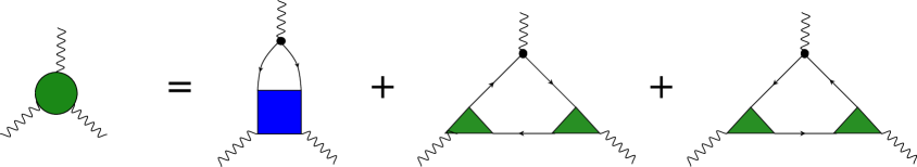
Figure 10: (Color online) Graph of the skeleton equation (A3) for the three-legged bosonic vertex.

Let us check a known limit of this equation. After replacing the exact propagators $G^{\alpha}(K)$ by $G_{0}^{\alpha}(K)$, the exact vertices $\Gamma^{\bar{\psi}^{\alpha}\psi^{\alpha}\phi}(K_{1};K_{2};\bar{K})$ by the bare vertices $\Gamma_{0}^{\alpha}$, and neglecting the contribution involving $\Gamma^{\bar{\psi}^{\alpha}\psi^{\alpha}\phi\phi}(K_{1};K_{2};\bar{K}_{1},\bar{K}_{2})$, we obtain from Eq. (A3)

$$\Gamma_{0}^{\phi\phi\phi}(\bar{K}_{1},\bar{K}_{2},-\bar{K}_{1}-\bar{K}_{2})=N\sum_{\alpha}\left(\Gamma_{0}^{\alpha}\right)^{3}\left[\int_{K}G_{0}^{\alpha}(K)G_{0}^{\alpha}(K+\bar{K}_{1})G_{0}^{\alpha}(K+\bar{K}_{1}+\bar{K}_{2})\right.$$

$$\qquad\qquad\qquad\qquad\qquad\qquad\qquad\qquad\left.{}+\int_{K}G_{0}^{\alpha}(K)G_{0}^{\alpha}(K+\bar{K}_{1})G_{0}^{\alpha}(K-\bar{K}_{2})\right],$$ (A4)

which is invariant under arbitrary permutations of $\bar{K}_{1}$, $\bar{K}_{2}$, and $\bar{K}_{3}=-\bar{K}_{1}-\bar{K}_{2}$. In fact, in this approximation, the bosonic three-legged vertex can be identified with the symmetrized closed fermion loop with three external legs and bare propagators given in Eq. (B1). As concerns Eq. (A3), the symmetry under permutations of its arguments is less obvious. However, as the left-hand side of Eq. (A2) is symmetric under permutations, and because all manipulations are exact, Eq. (A3) indeed fulfills this symmetry.

To obtain the approximation for the bosonic three-loop used in Sec. V, we adopt the same approximation strategy as in the skeleton approximation used for the bosonic self-energy: replacing the vertices $\Gamma^{\bar{\psi}^{\alpha}\psi^{\alpha}\phi}(K_{1};K_{2};\bar{K})$ and $\Gamma^{\bar{\psi}^{\alpha}\psi^{\alpha}\phi\phi}(K_{1};K_{2};\bar{K}_{1},\bar{K}_{2})$ by the bare vertices $\Gamma_{0}^{\alpha}$ and $0$, but retaining dressed propagators $G^{\alpha}(K)$, we arrive at Eqs. (85) and (86).

Appendix B: The symmetrized three-loop

In the momentum-transfer cutoff scheme, all irreducible vertices involving only bosonic external legs are finite at the initial scale and can be identified by the symmetrized closed fermion loops with bare fermionic propagators. In particular, the initial condition for the vertex with three external boson legs is

$$\Gamma^{\phi\phi\phi}_{0}(\bar{K}_{1},\bar{K}_{2},\bar{K}_{3})=2!N\sum_{\alpha}(\Gamma_{0}^{\alpha})^{3}L^{\alpha}_{3}(-\bar{K}_{1},-\bar{K}_{2},-\bar{K}_{3}),$$ (B1)

where the symmetrized three-loop $L^{\alpha}_{3}(\bar{K}_{1},\bar{K}_{2},\bar{K}_{3})$ can be expressed in terms of the non-symmetrized three-loop $\bar{L}^{\alpha}_{3}(\bar{K}_{1},\bar{K}_{2},\bar{K}_{3})$, defined by

$$\bar{L}^{\alpha}_{3}(\bar{K}_{1},\bar{K}_{2},\bar{K}_{3})=\int_{K}G_{0}^{\alpha}(K-\bar{K}_{1})G_{0}^{\alpha}(K-\bar{K}_{2})G_{0}^{\alpha}(K-\bar{K}_{3})$$ (B2)

as follows,

$$L^{\alpha}_{3}(\bar{K}_{1},\bar{K}_{2},\bar{K}_{3})$$ (B3)

$$= \frac{1}{3!}\Bigl{[}\bar{L}^{\alpha}_{3}(\bar{K}_{1},\bar{K}_{1}+\bar{K}_{2},0)+\bar{L}^{\alpha}_{3}(\bar{K}_{2},\bar{K}_{1}+\bar{K}_{2},0)$$

$$\hskip 8.53581pt+\bar{L}^{\alpha}_{3}(\bar{K}_{2},\bar{K}_{2}+\bar{K}_{3},0)+\bar{L}^{\alpha}_{3}(\bar{K}_{3},\bar{K}_{2}+\bar{K}_{3},0)$$

$$\hskip 8.53581pt+\bar{L}^{\alpha}_{3}(\bar{K}_{3},\bar{K}_{3}+\bar{K}_{1},0)+\bar{L}^{\alpha}_{3}(\bar{K}_{1},\bar{K}_{3}+\bar{K}_{1},0)\Bigr{]}.\hskip 25.60747pt$$

Actually, taking into account energy-momentum conservation, we may set $\bar{K}_{3}=-\bar{K}_{1}-\bar{K}_{2}$, so that we need

$$L^{\alpha}_{3}(\bar{K}_{1},\bar{K}_{2},-\bar{K}_{1}-\bar{K}_{2})$$ (B4)

$$= \frac{1}{3!}\Bigl{[}\bar{L}^{\alpha}_{3}(\bar{K}_{1},\bar{K}_{1}+\bar{K}_{2},0)+\bar{L}^{\alpha}_{3}(-\bar{K}_{1},-\bar{K}_{1}-\bar{K}_{2},0)$$

$$\hskip 8.53581pt+\bar{L}^{\alpha}_{3}(\bar{K}_{2},\bar{K}_{1}+\bar{K}_{2},0)+\bar{L}^{\alpha}_{3}(-\bar{K}_{2},-\bar{K}_{1}-\bar{K}_{2},0)$$

$$\hskip 8.53581pt+\bar{L}^{\alpha}_{3}(\bar{K}_{1},-\bar{K}_{2},0)+\bar{L}^{\alpha}_{3}(-\bar{K}_{1},\bar{K}_{2},0)\Bigr{]}.$$

For our model, the three-loops can be calculated analytically using the method outlined in the appendix of Ref. Pirooznia et al., 2008. Consider first the non-symmetrized three-loop defined in Eq. (B2). To perform the loop integration, we decompose the integrand in partial fractions, then carry out the $k_{\parallel}$ integration by means of the method of residues, and finally perform the $\omega$-integration. Using the notation $\bar{K}_{i}=(i\bar{\omega}_{i},\bar{\bm{k}}_{i})$, the result can be written as

$$\bar{L}^{\alpha}_{3}(\bar{K}_{1},\bar{K}_{2},\bar{K}_{3})=\frac{1}{2\pi}\int\frac{dk_{\bot}}{2\pi}\sum_{i=1}^{3}i\bar{\omega}_{i}\prod_{\stackrel{{\scriptstyle j=1}}{{j\neq i}}}^{3}\frac{1}{\Omega^{\alpha}_{ij}(k_{\bot})}$$

$$=\frac{1}{2\pi}\int\frac{dk_{\bot}}{2\pi}\Biggl{[}\frac{i\bar{\omega}_{1}}{\Omega_{12}^{\alpha}(k_{\bot})\Omega_{13}^{\alpha}(k_{\bot})}+\frac{i\bar{\omega}_{2}}{\Omega_{23}^{\alpha}(k_{\bot})\Omega_{21}^{\alpha}(k_{\bot})}$$

$$\hskip 56.9055pt+\frac{i\bar{\omega}_{3}}{\Omega_{31}^{\alpha}(k_{\bot})\Omega_{32}^{\alpha}(k_{\bot})}\Biggr{]},$$ (B5)

where we have defined

$$\Omega^{\alpha}_{ij}({k}_{\bot})=i\bar{\omega}_{i}-i\bar{\omega}_{j}+\xi^{\alpha}_{\bm{k}-\bar{\bm{k}}_{i}}-\xi^{\alpha}_{\bm{k}-\bar{\bm{k}}_{j}}$$

$$=i\omega_{ij}-\alpha(\bar{k}_{\parallel i}-\bar{k}_{\parallel j})+(\bar{k}_{\bot i}^{2}-\bar{k}_{\bot j}^{2})-2q_{ij}k_{\bot}$$

$$=-2q_{ij}[k_{\bot}-k_{ij}],$$ (B6)

with

$$\omega_{ij} = \bar{\omega}_{i}-\bar{\omega}_{j}\;\;,\;\;q_{ij}=\bar{k}_{\bot i}-\bar{k}_{\bot j},$$ (B7a)

$$k_{ij} = \frac{\bar{k}_{\bot i}+\bar{k}_{\bot j}}{2}+\frac{i\omega_{ij}-\alpha(\bar{k}_{\parallel i}-\bar{k}_{\parallel j})}{2q_{ij}}.$$ (B7b)

The remaining $k_{\bot}$-integration in Eq. (B5) can now be done using the residue theorem and we finally obtain

$$\bar{L}^{\alpha}_{3}(\bar{K}_{1},\bar{K}_{2},\bar{K}_{3}) = -\frac{1}{8\pi}\Biggl{[}$$ (B8)

$$\frac{\bar{\omega}_{1}}{q_{12}q_{13}}\frac{\Theta({\rm Im}(k_{12}))-\Theta({\rm Im}(k_{13}))}{k_{12}-k_{13}}$$

$$+ \frac{\bar{\omega}_{2}}{q_{23}q_{21}}\frac{\Theta({\rm Im}(k_{23}))-\Theta({\rm Im}(k_{21}))}{k_{23}-k_{21}}$$

$$+ \frac{\bar{\omega}_{3}}{q_{31}q_{32}}\frac{\Theta({\rm Im}(k_{31}))-\Theta({\rm Im}(k_{32}))}{k_{31}-k_{32}}\Biggr{]}.\hskip 19.91692pt$$

Substituting this expression into Eq. (B4) and defining

$$x_{i} = \frac{\bar{\omega}_{i}}{\bar{k}_{\bot i}}\;\;,\;\;s_{i}=\frac{\bar{k}_{\bot i}}{\bar{k}_{\bot 1}+\bar{k}_{\bot 2}},$$ (B9)

we obtain for the symmetrized three-loop,

$$L^{\alpha}_{3}(\bar{K}_{1},\bar{K}_{2},-\bar{K}_{1}-\bar{K}_{2}) = \frac{1}{3!2\pi}\frac{1}{s_{1}s_{2}\left[\frac{\bar{k}_{\parallel 1}}{\bar{k}_{\bot 1}}-\frac{\bar{k}_{\parallel 2}}{\bar{k}_{\bot 2}}-i\alpha(x_{1}-x_{2})\right]^{2}-\bar{k}_{\bot 1}\bar{k}_{\bot 2}}\Biggl{[}\bigl{(}s_{1}|x_{1}|+s_{2}|x_{2}|\bigr{)}\Theta(-x_{1}x_{2})$$ (B10)

$$+\bigl{(}s_{1}|x_{1}|-|s_{1}x_{1}+s_{2}x_{2}|\bigr{)}\Theta(-x_{1}(s_{1}x_{1}+s_{2}x_{2}))+\bigl{(}s_{2}|x_{2}|-|s_{1}x_{1}+s_{2}x_{2}|\bigr{)}\Theta(-x_{2}(s_{1}x_{1}+s_{2}x_{2}))\Biggr{]}.$$

Alternatively, this expression can be written as

$$L^{\alpha}_{3}(\bar{K}_{1},\bar{K}_{2},-\bar{K}_{1}-\bar{K}_{2}) = \frac{1}{3!2\pi}\frac{1}{s_{1}s_{2}\left[\frac{\bar{k}_{\parallel 1}}{\bar{k}_{\bot 1}}-\frac{\bar{k}_{\parallel 2}}{\bar{k}_{\bot 2}}-i\alpha(x_{1}-x_{2})\right]^{2}-\bar{k}_{\bot 1}\bar{k}_{\bot 2}}\Biggl{[}\bigl{(}s_{1}x_{1}-s_{2}x_{2}\bigr{)}[\Theta(x_{1})-\Theta(x_{2})]$$ (B11)

$$+\bigl{(}2s_{1}x_{1}+s_{2}x_{2}\bigr{)}[\Theta(x_{1})-\Theta(s_{1}x_{1}+s_{2}x_{2})]+\bigl{(}2s_{2}x_{2}+s_{1}x_{1}\bigr{)}[\Theta(x_{2})-\Theta(s_{1}x_{1}+s_{2}x_{2})]\Biggr{]}$$

$$= \frac{1}{4\pi}\frac{s_{1}x_{1}\Theta(x_{1})+s_{2}x_{2}\Theta(x_{2})-(s_{1}x_{1}+s_{2}x_{2})\Theta(s_{1}x_{1}+s_{2}x_{2})}{s_{1}s_{2}\left[\frac{\bar{k}_{\parallel 1}}{\bar{k}_{\bot 1}}-\frac{\bar{k}_{\parallel 2}}{\bar{k}_{\bot 2}}-i\alpha(x_{1}-x_{2})\right]^{2}-\bar{k}_{\bot 1}\bar{k}_{\bot 2}}$$

$$= \frac{1}{4\pi}\left(\frac{1}{\bar{k}_{\bot 1}}+\frac{1}{\bar{k}_{\bot 2}}\right)\frac{\bar{\omega}_{1}\Theta\left(\frac{\bar{\omega}_{1}}{\bar{k}_{\bot 1}}\right)+\bar{\omega}_{2}\Theta\left(\frac{\bar{\omega}_{2}}{\bar{k}_{\bot 2}}\right)-(\bar{\omega}_{1}+\bar{\omega}_{2})\Theta\left(\frac{\bar{\omega}_{1}+\bar{\omega}_{2}}{\bar{k}_{\bot 1}+\bar{k}_{\bot 2}}\right)}{\left[\frac{\bar{k}_{\parallel 1}}{\bar{k}_{\bot 1}}-\frac{\bar{k}_{\parallel 2}}{\bar{k}_{\bot 2}}-i\alpha(\frac{\bar{\omega}_{1}}{\bar{k}_{\bot 1}}-\frac{\bar{\omega}_{2}}{\bar{k}_{\bot 2}})\right]^{2}-(\bar{k}_{\bot 1}+\bar{k}_{\bot 2})^{2}}.$$

For a different effective model for the nematic quantum critical point involving a quadratic energy dispersion (and hence a compact Fermi surface) the scaling properties of fermion loops have recently been analyzed by Thier and Metzner Thier and Metzner (2011), who found that also in this case the fermion loops exhibit a singular dependence on momenta and frequencies. However, to obtain consistent scaling properties of the effective interactions between bosonic fluctuations described by the fermion loops, one should use one-loop renormalized fermion propagators $G^{\alpha}(K)=\frac{Z}{i\omega-Z\xi^{\alpha}_{\bm{k}}}$ in the loop integrations, which can be formally justified from the skeleton equation for the irreducible vertex with three external bosonic legs, as discussed in Appendix A. The corresponding expression for the renormalized three-loop can be obtained from Eq. (B11) by replacing all external frequencies by $\bar{\omega}\rightarrow\bar{\omega}/Z$ and multiplying the loop by an overall factor of $Z$. The result is given in Eq. (86).

References

- Ando et al. (2002) Y. Ando, K. Segawa, S. Komiya, and A. N. Lavrov, Phys. Rev. Lett. 88, 137005 (2002).
- Borzi et al. (2007) R. A. Borzi, S. A. Grigera, J. Farrell, R. S. Perry, S. J. S. Lister, S. L. Lee, D. A. Tennant, Y. Maeno, and A. P. Mackenzie, Science 315, 214 (2007).
- Kohsaka et al. (2007) Y. Kohsaka, C. Taylor, K. Fujita, A. Schmidt, C. Lupien, T. Hanaguri, M. Azuma, M. Takano, H. Eisaki, H. Takagi, S. Uchida, and J. C. Davis, Science 315, 1380 (2007).
- Hinkov et al. (2008) V. Hinkov, D. Haug, B. Fauqué, P. Bourges, Y. Sidis, A. Ivanov, C. Bernhard, C. T. Lin, and B. Keimer, Science 319, 597 (2008).
- Daou et al. (2010) R. Daou, J. Chang, D. LeBoeuf, O. Cyr-Choinière, F. Laliberté, N. Doiron-Leyraud, B. Ramshaw, R. Liang, D. Bonn, W. Hardy, and L. Taillefer, Nature 463, 519 (2010).
- Nandi et al. (2010) S. Nandi, M. G. Kim, A. Kreyssig, R. M. Fernandes, D. K. Pratt, A. Thaler, N. Ni, S. L. Bud’ko, P. C. Canfield, J. Schmalian, R. J. McQueeney, and A. I. Goldman, Phys. Rev. Lett. 104, 057006 (2010).
- Fradkin et al. (2010) E. Fradkin, S. A. Kivelson, M. J. Lawler, J. P. Eisenstein, and A. P. Mackenzie, Annu. Rev. Cond. Mat. Phys. 1, 153 (2010).
- Pomeranchuk (1958) I. Pomeranchuk, Soviet. Phys. JETP 8, 361 (1958).
- Halboth and Metzner (2000) C. J. Halboth and W. Metzner, Phys. Rev. Lett. 85, 5162 (2000).
- Hertz (1976) J. A. Hertz, Phys. Rev. B 14, 1165 (1976).
- Millis (1993) A. J. Millis, Phys. Rev. B 48, 7183 (1993).
- Belitz et al. (2005) D. Belitz, T. R. Kirkpatrick, and T. Vojta, Rev. Mod. Phys. 77, 579 (2005).
- Löhneysen et al. (2007) H. v. Löhneysen, A. Rosch, M. Vojta, and P. Wölfle, Rev. Mod. Phys. 79, 1015 (2007).
- Vojta (2003) M. Vojta, Rep. Prog. Phys. 66, 2069 (2003).
- Holstein et al. (1973) T. Holstein, R. E. Norton, and P. Pincus, Phys. Rev. B 8, 2649 (1973).
- Reizer (1989) M. Y. Reizer, Phys. Rev. B 40, 11571 (1989).
- Lee and Nagaosa (1992) P. A. Lee and N. Nagaosa, Phys. Rev. B 46, 5621 (1992).
- Halperin et al. (1993) B. I. Halperin, P. A. Lee, and N. Read, Phys. Rev. B 47, 7312 (1993).
- Motrunich (2005) O. I. Motrunich, Phys. Rev. B 72, 045105 (2005).
- Lee and Lee (2005) S.-S. Lee and P. A. Lee, Phys. Rev. Lett. 95, 036403 (2005).
- Rech et al. (2006) J. Rech, C. Pépin, and A. V. Chubukov, Phys. Rev. B 74, 195126 (2006).
- Gonzáles et al. (1994) J. Gonzáles, F. Guinea, and M. A. H. Vozmediano, Nucl. Phys. B 424, 595 (1994).
- Giuliani et al. (2010) A. Giuliani, V. Mastropietro, and M. Porta, Phys. Rev. B 82, 121418(R) (2010).
- Altshuler et al. (1994) B. L. Altshuler, L. B. Ioffe, and A. J. Millis, Phys. Rev. B 50, 14048 (1994).
- Polchinski (1994) J. Polchinski, Nucl. Phys. B 422, 617 (1994).
- Sedrakyan and Chubukov (2011) T. A. Sedrakyan and A. V. Chubukov, Phys. Rev. B 79, 115129 (2009).
- Lee (2008) S.-S. Lee, Phys. Rev. B 78, 085129 (2008).
- Lee (2009) S.-S. Lee, Phys. Rev. B 80, 165102 (2009).
- Metlitski and Sachdev (2010a) M. A. Metlitski and S. Sachdev, Phys. Rev. B 82, 075127 (2010a).
- Metlitski and Sachdev (2010b) M. A. Metlitski and S. Sachdev, Phys. Rev. B 82, 075128 (2010b).
- Chubukov (2010) A. V. Chubukov, Physics 3, 70 (2010).
- Mross et al. (2010) D. F. Mross, J. McGreevy, H. Liu, and T. Senthil, Phys. Rev. B 82, 045121 (2010).
- Nayak and Wilczek (1994a) C. Nayak and F. Wilczek, Nucl. Phys. B 417, 359 (1994a).
- Nayak and Wilczek (1994b) C. Nayak and F. Wilczek, Nucl. Phys. B 430, 534 (1994b).
- Wetterich (1993) C. Wetterich, Phys. Lett. B 301, 90 (1993).
- Berges et al. (2002) J. Berges, N. Tetradis, and C. Wetterich, Phys. Rep. 363, 223 (2002).
- Kopietz et al. (2010) P. Kopietz, L. Bartosch, and F. Schütz, Introduction to the Functional Renormalization Group (Springer, Berlin, 2010).
- Metzner et al. (2012) W. Metzner, M. Salmhofer, C. Honerkamp, V. Meden, and K. Schönhammer, Rev. Mod. Phys. 84, 299 (2012).
- Baier et al. (2004) T. Baier, E. Bick, and C. Wetterich, Phys. Rev. B 70, 125111 (2004).
- Baier et al. (2005) T. Baier, E. Bick, and C. Wetterich, Phys. Lett. B 605, 144 (2005).
- Schütz et al. (2005) F. Schütz, L. Bartosch, and P. Kopietz, Phys. Rev. B 72, 035107 (2005).
- Wetterich (2007) C. Wetterich, Phys. Rev. B 75, 085102 (2007).
- Strack et al. (2008) P. Strack, R. Gersch, and W. Metzner, Phys. Rev. B 78, 014522 (2008).
- Bartosch et al. (2009a) L. Bartosch, H. Freire, J. J. Ramos Cardenas, and P. Kopietz, J. Phys.: Condens. Matter 21, 305602 (2009a).
- Bartosch et al. (2009b) L. Bartosch, P. Kopietz, and A. Ferraz, Phys. Rev. B 80, 104514 (2009b).
- Sachdev (2011) S. Sachdev, Quantum Phase Transitions (Cambridge University Press, Cambridge, 2011), 2nd ed.
- Yamamoto and Si (2010) S. J. Yamamoto and Q. Si, Phys. Rev. B 81, 205106 (2010).
- Isidori et al. (2010) A. Isidori, D. Roosen, L. Bartosch, W. Hofstetter, and P. Kopietz, Phys. Rev. B 81, 235120 (2010).
- Pirooznia et al. (2008) P. Pirooznia, F. Schütz, and P. Kopietz, Phys. Rev. B 78, 075111 (2008).
- Thier and Metzner (2011) S. C. Thier and W. Metzner, Phys. Rev. B 84, 155133 (2011).