Rossby wave instability in locally isothermal and polytropic disks: three-dimensional linear calculations

Abstract

Numerical calculations of the linear Rossby wave instability (RWI) in global three-dimensional (3D) disks are presented. The linearized fluid equations are solved for vertically stratified, radially structured disks with either a locally isothermal or polytropic equation of state, by decomposing the vertical dependence of the perturbed hydrodynamic quantities into Hermite and Gegenbauer polynomials, respectively. It is confirmed that the RWI operates in 3D. For perturbations with vertical dependence assumed above, there is little difference in growth rates between 3D and two-dimensional (2D) calculations. Comparison between 2D and 3D solutions of this type suggest the RWI is predominantly a 2D instability and that three-dimensional effects, such as vertical motion, to be interpreted as a perturbative consequence of the dominant 2D flow. The vertical flow around co-rotation, where vortex-formation is expected, is examined. In locally isothermal disks the expected vortex center remains in approximate vertical hydrostatic equilibrium. For polytropic disks the vortex center has positive vertical velocity, whose magnitude increases with decreasing polytropic index $n$.

Email: ]mklin924@cita.utoronto.ca

1. Introduction

Theoretical modeling of protoplanetary disks lead to complex structures that are unlikely to be described by smooth radial profiles (Terquem, 2008; Armitage, 2011). However, radially structured disks may develop the Rossby wave instability (RWI, Lovelace et al., 1999; Li et al., 2000), which leads to vortex-formation in the nonlinear regime (Li et al., 2001). Thus, the RWI may play a role in the evolution of protoplanetary disks.

The disk RWI is a dynamical instability associated with the presence of extrema in the ratio of vorticity to surface density, or vortensity. The instability results from wave coupling across such an extremum. Its physics is similar to the Papaloizou-Pringle instability (PPI, Papaloizou & Pringle, 1984, 1985, 1987; Goldreich et al., 1986; Narayan et al., 1987) which operate in pressure-supported, thick tori. The RWI operates in thin, centrifugally-supported disks with non-power law rotation profiles, and is insensitive to radial boundary conditions.

The relevance of the RWI in protoplanetary disks has been demonstrated in two situations. Variability in the efficiency of turbulent angular momentum transport by the magneto-rotational instability (Balbus & Hawley, 1991) can result in the existence of ‘dead zones’ (Gammie, 1996), in which the turbulent viscosity is small. The radial boundary between a dead zone and the actively accreting region is prone to the RWI (Varnière & Tagger, 2006; Lyra et al., 2008, 2009; Crespe et al., 2011), with observable consequences (Regály et al., 2012). In addition to hydrodynamic angular momentum transport, the RWI may also assist planet formation formation by concentrating solids into anti-cyclonic vortices (Barge & Sommeria, 1995).

Another origin of the RWI in protoplanetary disks, which motivated this study, is disk-planet interaction (Goldreich & Tremaine, 1979, 1980). A sufficiently massive planet leads to gap opening (Lin & Papaloizou, 1986), while low mass protoplanets may open gaps provided the disk viscosity is sufficiently small (Muto et al., 2010; Dong et al., 2011). Vortensity jumps across planet-induced shocks lead to the necessary disk profile for the RWI to develop around gap edges (Koller et al., 2003; Li et al., 2005; de Val-Borro et al., 2007). Subsequent vortex-formation significantly affects disk-planet torques and migration (Ou et al., 2007; Li et al., 2009; Yu et al., 2010; Lin & Papaloizou, 2010).

The above studies of the RWI have all employed the razor-thin disk approximation (but note that the PPI was originally analyzed in 3D). Yu & Li (2009) have examined the RWI with a toroidal magnetic field in a 3D but unstratified disk. Meheut et al. (2010) first demonstrated the RWI in nonlinear hydrodynamic simulations of 3D stratified disks ( later with improved resolution in Meheut et al., 2012a), while Umurhan (2010) analyzed the RWI in approximate 3D disk models.

Recently, Meheut et al. (2012b) calculated linear RWI modes in a three-dimensional, globally isothermal disk, which displayed vertical motion. In this paper, we compute linear RWI modes in three-dimensional disks across a range of parameter values, including different equations of state. Our focus here is on how these affect the vertical flow in the co-rotation region, where vortex-formation is known to occur (Li et al., 2001).

This paper is organized as follows. In §2 we list the governing equations and describe our disk models. We derive the linearized fluid equations in §3 and describe our numerical methods in §4. Results are presented in §5 for locally isothermal disks and in §6 for polytropic disks. In §7 we briefly examine a linear mode qualitatively different to those above, found in a disk model involving $\kappa^{2}<0$ (taken from Meheut et al., 2010), where $\kappa$ is the epicycle frequency. We summarize and discuss our results in §8, including limitations of our calculations.

2. Governing equations, disk models and assumptions

We consider a three-dimensional, inviscid, non-self-gravitating disk orbiting a star of mass $M_{*}$ and adopt $(r,\phi,z)$ cylindrical polar co-ordinates centered on the star. The frame is non-rotating. The governing equations are the 3D Euler equations:

$$\frac{\partial\rho}{\partial t}+\nabla\cdot(\rho\bm{v})=0,$$ (1)

$$\frac{\partial\bm{v}}{\partial t}+\bm{v}\cdot\nabla\bm{v}=-\frac{1}{\rho}\nabla P-\nabla\Phi_{*},$$ (2)

$$P=P(r,\rho),$$ (3)

where $\rho$ is the density, $P$ is the pressure, $\bm{v}$ is the velocity field and $\Phi_{*}$ is the gravitational potential due to the central star. Eq. 3 is an equation of state (EOS), specified later, such that the pressure may be calculated without an energy equation.

We assume the disk is geometrically thin so that $\Phi_{*}$ may be approximated as

$$\Phi_{*}(r,z)=-\frac{GM_{*}}{\sqrt{r^{2}+z^{2}}}\simeq-\frac{GM_{*}}{r}\left(1-\frac{z^{2}}{2r^{2}}\right).$$ (4)

This approximation is adopted so that the resulting equilibrium density field has a convenient functional form suitable for the application of orthogonal polynomials (see §4). This greatly simplifies the numerical problem. Henceforth we use the approximate potential for self-consistency.

The unperturbed disk is steady, axisymmetric with no meridional velocity ($\partial_{t}=\partial_{\phi}=v_{r}=v_{z}=0$). The disk is stratified with $\rho=\rho(r,z)$ set by vertical hydrostatic balance. The azimuthal velocity is $v_{\phi}=r\Omega$, where $\Omega$ is the angular speed. $v_{\phi}$ is set by radial balance between pressure, stellar gravity and centrifugal forces. Because the disk is thin, the angular velocity is close to Keplerian, i.e. $\Omega\simeq\Omega_{k}\equiv(GM_{*}/r^{3})^{1/2}$.

To introduce radial structure, we choose the unperturbed surface density profile to be

$$\Sigma(r) \equiv\int^{\infty}_{-\infty}\rho dz$$

$$=\Sigma_{0}\left(\frac{r}{r_{0}}\right)^{-\alpha}\left\{1+(\mathcal{A}-1)\exp{\left[-\frac{(r-r_{0})^{2}}{2\Delta r^{2}}\right]}\right\}$$ (5)

(Li et al., 2000). Eq. 2 corresponds to a Gaussian surface density bump centered at $r=r_{0}$, width $\Delta r$ and amplitude $\mathcal{A}$, on top of a background power-law profile with index $-\alpha$. Since disk self-gravity is ignored, the surface density scale $\Sigma_{0}$ is arbitrary.

To specify the three-dimensional disk structure, we choose the EOS to be either locally isothermal or polytropic. These are described below.

2.1. Locally isothermal disks

For locally isothermal disks the pressure is calculated as

$$P=c_{s}^{2}(r)\rho,$$ (6)

where $c_{s}(r)$ is the sound-speed given by $c_{s}=H\Omega_{k}$ and $H(r)$ is the disk scale-height. The unperturbed density is

$$\rho(r,z)=\frac{\Sigma(r)}{\sqrt{2\pi}H(r)}\exp{\left[-\frac{z^{2}}{2H^{2}(r)}\right]}.$$ (7)

In the numerical calculations we will choose $H(r)=hr$ with $h$ being a constant aspect-ratio, since this is a typical model for protoplanetary disks. The exponential decay means the gas density becomes negligible after a few scale heights. Thus the vertical domain can be taken to be $z\in[-\infty,\infty]$, even though we have made the thin-disk approximation.

2.1.1 Approximate equilibrium

For simplicity, we set the azimuthal velocity to

$$v_{\phi}^{2}=\left.\frac{r}{\rho}\frac{\partial P}{\partial r}\right|_{z=0}+r\left.\frac{\partial\Phi_{*}}{\partial r}\right|_{z=0}.$$ (8)

Away from the midplane the deviation from exact radial balance is proportional to $h^{2}\ll 1$ for a thin disk (Tanaka et al., 2002). We adopt Eq. 8 to allow us to apply standard solution methods.

To test whether or not the precise form of $\Omega$ affect our results, we also considered setting $\rho\to\Sigma$ in Eq. 8, which gives the velocity profile $v_{\phi,\mathrm{2D}}$ for a razor-thin disk. For our fiducial calculation, growth rates differ by $\sim 1\%$ between adopting Eq. 8 or $v_{\phi,\mathrm{2D}}$, and we observe the same flow structure.

In fact, locally isothermal disks generally have differential rotation in $z$, i.e. $\Omega=\Omega(r,z)$, unless the disk is also globally isothermal. It is therefore important to note that in assuming Eq. 8 , we have artificially suppressed baroclinic effects. We discuss some justification for this in §8.4 and Appendix A. Although the chosen basic state is not in exact equilibrium, setting $\Omega=\Omega(r)$ greatly simplifies the linear equations as the only vertical dependence of the basic state is through the exponential factor in $\rho$. It allows us to address the specific question of whether or not vertical density stratification has any effect on the RWI, without the complication of baroclinic instabilities (Knobloch & Spruit, 1986; Umurhan, 2012).

2.2. Polytropic disks

In order to set up a more self-consistent basic state, that is, $\Omega=\Omega(r)$ and a finite vertical domain, we also consider polytropic disks, for which

$$P=K\rho^{1+\frac{1}{n}},$$ (9)

where $K$ is a constant and $n$ is the polytropic index. Vertical hydrostatic equilibrium imply

$$\rho(r,z) =\left[\frac{GM_{*}H^{2}(r)}{2K(1+n)r^{3}}\right]^{n}\left[1-\frac{z^{2}}{H^{2}(r)}\right]^{n}$$

$$\equiv\rho_{0}(r)\left[1-\frac{z^{2}}{H^{2}(r)}\right]^{n}$$ (10)

Here, $z=H$ is the disk surface where $\rho(r,H)=0$. Thus, when discussing polytropic disks $H$ is referred to as the disk thickness.

The function $H(r)$ and mid-plane density $\rho_{0}(r)$ are calculated through

$$\Sigma(r)=\rho_{0}(r)H(r)I_{n},$$ (11)

where $I_{n}\equiv\int^{1}_{-1}(1-x^{2})^{n}dx$, with $\rho_{0}(r)$ related to $H(r)$ by Eq. 2.2 and $\Sigma(r)$ given by Eq. 2. We can therefore write

$$H(r)=H_{0}\left[\frac{\Sigma(r)}{\mathcal{A}\Sigma_{0}}\right]^{\frac{1}{2n+1}}\left(\frac{r}{r_{0}}\right)^{\frac{3n}{2n+1}},$$ (12)

where $H_{0}=H(r_{0})$ is the disk thickness at the bump radius. We parametrize it by writing $H_{0}=hr_{0}$ so that $h$ is the aspect-ratio at $r_{0}$. Note that a surface density enhancement by a factor $\mathcal{A}$ corresponds to an enhancement of the disk thickness by a factor $\mathcal{A}^{1/(2n+1)}$.

For a polytropic disk the azimuthal velocity is strictly independent of $z$ (e.g. Papaloizou & Pringle, 1984). It is given by

$$v_{\phi}^{2}(r)=r\frac{\partial}{\partial r}\Phi_{*}(r,H)=\frac{GM_{*}}{r}\left(1-\frac{3H^{2}}{2r^{2}}+\frac{H}{r}\frac{dH}{dr}\right),$$ (13)

where the second equality follows from the approximation for the stellar potential in a thin disk (Eq. 4).

Of course, given $H(r)$ one can obtain the azimuthal velocity $v_{\phi,e}$ corresponding to the exact gravitational potential of a point mass. For our fiducial setup, the difference in growth rate is $<4\%$ between using $v_{\phi,e}$ and using $v_{\phi}$ above, and we observe no difference in flow structure. However, we will use $v_{\phi}$ so that the equilibrium density and velocity fields are self-consistent and in exact balance with the same potential.

3. Linearized equations

In this section we derive the governing equation for small disturbances in the disk. As described above, the basic state is $\rho=\rho(r,z)$ and $\bm{v}=(0,r\Omega,0)$, with $\Omega=\Omega(r)$. The perturbed state is assumed to have the form

$$\rho \to\rho+\operatorname{Re}[\delta\rho(r,z)\exp{\mathrm{i}(\sigma t+m\phi)}],$$ (14)

$$P \to P+\operatorname{Re}[\delta P(r,z)\exp{\mathrm{i}(\sigma t+m\phi)}],$$ (15)

$$\bm{v} \to\bm{v}+\operatorname{Re}[\delta\bm{v}(r,z)\exp{\mathrm{i}(\sigma t+m\phi)}],$$ (16)

where $\sigma=\sigma_{R}+\mathrm{i}\gamma$ is a complex frequency ($\sigma_{R},\,\gamma$ being real) and $m$ is the azimuthal wave-number taken to be a positive integer. We will omit writing ‘$\operatorname{Re}$’ below, with the understanding that physical solutions correspond to real parts of the complex perturbations.

For the locally isothermal equation of state, the linearized momentum equations give

$$\delta v_{r}=-\frac{\mathrm{i}c_{s}^{2}}{D}\left(\bar{\sigma}\frac{\partial W}{\partial r}+\frac{2m\Omega W}{r}\right),$$ (17)

$$\delta v_{\phi}=\frac{c_{s}^{2}}{D}\left(\frac{\kappa^{2}}{2\Omega}\frac{\partial W}{\partial r}+\frac{\bar{\sigma}mW}{r}\right),$$ (18)

$$\delta v_{z}=\frac{\mathrm{i}c_{s}^{2}}{\bar{\sigma}}\frac{\partial W}{\partial z},$$ (19)

where $W\equiv\delta\rho/\rho$ is the relative density perturbation, $\bar{\sigma}\equiv\sigma+m\Omega(r)$ is the shifted frequency, $D\equiv\kappa^{2}-\bar{\sigma}^{2}$, and

$$\kappa^{2}=\frac{1}{r^{3}}\frac{\partial}{\partial r}\left(r^{4}\Omega^{2}\right)$$ (20)

is the square of the epicycle frequency. Corresponding equations for the polytropic disk are very similar, and are readily obtained by setting $c_{s}$ to unity and replacing $W\to S\equiv\delta P/\rho$ where $S$ is the enthalpy perturbation.

Inserting the perturbed velocity field into the linearized continuity equation

$$\mathrm{i}\bar{\sigma}\delta\rho+\frac{1}{r}\frac{\partial}{\partial r}\left(r\rho\delta v_{r}\right)+\frac{\mathrm{i}m}{r}\rho\delta v_{\phi}+\frac{\partial}{\partial z}\left(\rho\delta v_{z}\right)=0,$$ (21)

yields, for locally isothermal disks:

$$r\delta\rho= \frac{\partial}{\partial r}\left(\frac{r\rho c_{s}^{2}}{D}\frac{\partial W}{\partial r}\right)+\frac{2mW}{\bar{\sigma}}\frac{\partial}{\partial r}\left(\frac{c_{s}^{2}\rho\Omega}{D}\right)$$

$$-\left(\frac{m^{2}c_{s}^{2}\rho}{rD}\right)W-\frac{rc_{s}^{2}}{\bar{\sigma}^{2}}\frac{\partial}{\partial z}\left(\rho\frac{\partial W}{\partial z}\right),$$ (22)

and for polytropic disks:

$$r\delta\rho= \frac{\partial}{\partial r}\left(\frac{r\rho}{D}\frac{\partial S}{\partial r}\right)+\frac{2mS}{\bar{\sigma}}\frac{\partial}{\partial r}\left(\frac{\rho\Omega}{D}\right)$$

$$-\left(\frac{m^{2}\rho}{rD}\right)S-\frac{r}{\bar{\sigma}^{2}}\frac{\partial}{\partial z}\left(\rho\frac{\partial S}{\partial z}\right).$$ (23)

We remark that Eq. 3 is in fact valid for locally isothermal disks with any fixed sound-speed profile $c_{s}(r)$, assuming the equilibrium azimuthal velocity is independent of $z$ (Appendix A). Also note that Eq. 3 is actually valid for any barotropic EOS , i.e. whenever $P=P(\rho)$. The 3D problem is to solve Eq. 3—3, which will generally describe disturbances depending on $(r,\phi,z)$ and motion in all three directions.

3.1. Relation to the two-dimensional problem

We define the 2D problem as solving Eq. 3—3 subject to $\partial_{z}=0$. Denoting the corresponding solutions as $W_{\mathrm{2D}}(r),\,S_{\mathrm{2D}}(r)$ and inserting them into the governing equations yields, after vertical integration,

$$r\delta\Sigma= \frac{d}{dr}\left(\frac{r\Sigma c_{s}^{2}}{D}\frac{dW_{\mathrm{2D}}}{dr}\right)+\frac{2mW_{\mathrm{2D}}}{\bar{\sigma}}\frac{d}{dr}\left(\frac{c_{s}^{2}\Sigma\Omega}{D}\right)$$

$$-\left(\frac{m^{2}c_{s}^{2}}{rD}\right)\Sigma W_{\mathrm{2D}}$$ (24)

for locally isothermal disks and

$$r\delta\Sigma= \frac{d}{dr}\left(\frac{r\Sigma}{D}\frac{dS_{\mathrm{2D}}}{dr}\right)+\frac{2mS_{\mathrm{2D}}}{\bar{\sigma}}\frac{d}{dr}\left(\frac{\Sigma\Omega}{D}\right)$$

$$-\left(\frac{m^{2}\Sigma}{rD}\right)S_{\mathrm{2D}}$$ (25)

for polytropic disks, where $\delta\Sigma=\int^{\infty}_{-\infty}\delta\rho dz$ is the surface density perturbation. Note that $W_{\mathrm{2D}}=\delta\Sigma/\Sigma$ is the relative surface density perturbation, and $S_{\mathrm{2D}}=\delta\Pi/\Sigma$ where $\delta\Pi$ is the perturbation to the vertically integrated pressure ($\Pi=\int^{\infty}_{-\infty}Pdz$). Solutions to Eq. 3.1—3.1 describe disturbances which only depend on $(r,\phi)$ and there is no vertical motion.

As defined here, the 2D problem and 3D problem involves the same background disk, which is three-dimensional. However, the governing equation for linear disturbances in razor-thin disks have the same form as Eq. 3.1—3.1 when the razor-thin disk has a locally isothermal or barotropic EOS in the form $\Pi=c_{s}^{2}(r)\Sigma$ or $\Pi=\Pi(\Sigma)$, respectively.

3.2. Co-rotation singularity and the RWI

Inspection of the 2D equations, Eq. 3.1—3.1, reveal a potential singularity when $\bar{\sigma}(r_{c})=0$, where $r_{c}$ is the co-rotation radius defined by

$$\sigma_{R}+m\Omega(r_{c})=0.$$ (26)

This co-rotation singularity can be rendered ineffective if $r_{c}$ also satisfies

$$\frac{d}{dr}\left.\left(\frac{c_{s}^{2}}{\eta}\right)\right|_{r_{c}}=0\quad\text{for locally isothermal disks},$$ (27)

$$\frac{d}{dr}\left.\left(\frac{1}{\eta}\right)\right|_{r_{c}}=0\,\,\quad\text{for polytropic disks},$$ (28)

where

$$\eta\equiv\frac{\kappa^{2}}{2\Omega\Sigma}$$ (29)

is the vortensity. The quantity $\eta/c_{s}^{2}$ can be seen as a generalized vortensity (Li et al., 2000), but for convenience we will simply use ‘vortensity’ in the discussion below. Thus there can exist 2D neutral disturbances with co-rotation at a vortensity extremum, for which the 2D linear operator is real and regular everywhere.

Strictly speaking, co-rotation singularities only concern neutral disturbances ($\gamma=0$). In practice we are interested in growing solutions ($\gamma<0$) so such singularities do not arise in the numerical computation. Nevertheless, the discussion above is important because the growth rates we find are typically $|\gamma|\ll\Omega(r_{0})$. Furthermore, association of $r_{c}$ with a vortensity extremum forms the basis of the RWI.

In studies employing razor-thin disks, the RWI has largest disturbance amplitude in the co-rotation region where $|\bar{\sigma}^{2}|\ll\kappa^{2}$. It can be shown that such modes can only be unstable if there exists vortensity extrema in the disk (e.g. Lin & Papaloizou, 2010). Indeed, the RWI is found to have with co-rotation radius $r_{c}$ close to a vortensity minimum (Lovelace et al., 1999; Li et al., 2000; Lin & Papaloizou, 2011a).

It is precisely linear modes with the above properties which we wish to explore in 3D. However, we do not expect such modes to have significant $z$-dependence in their relative density or enthalpy perturbation around co-rotation. From the linearized vertical equation of motion we see that

$$\delta v_{z}\propto\frac{1}{\bar{\sigma}}\frac{\partial X}{\partial z},$$

where $X$ is $W$ or $S$ depending on the EOS. Near co-rotation where $|\bar{\sigma}|$ is small, $|\partial_{z}X|$ should be almost negligible. Otherwise, even small vertical gradients in density or enthalpy perturbation will cause significant vertical motion, and linearization becomes invalid.

4. Numerical procedure

In principle one could attempt a numerical solution to the partial differential equations (PDE) above, for example by finite-differencing in the $(r,z)$ plane. However, since one of our goals is to assess three-dimensional effects, it is more useful to have a numerical scheme that automatically separates out the 2D problem from the full 3D problem.

We begin by making the co-ordinate transformation

$$(\hat{r},\hat{z}) \equiv(r,z/H),$$ (30)

$$\left(\frac{\partial}{\partial r},\frac{\partial}{\partial z}\right) =\left(\frac{\partial}{\partial\hat{r}}-\hat{z}\frac{H^{\prime}}{H}\frac{\partial}{\partial\hat{z}},\frac{1}{H}\frac{\partial}{\partial\hat{z}}\right),$$ (31)

where ^′ denotes differentiation with respect to the argument. In this co-ordinate system the background density is separable, i.e. $\rho(\hat{r},\hat{z})=g(\hat{r})f(\hat{z})$, where $f=\exp{(-\hat{z}^{2}/2)}$ for locally isothermal disks and $f=(1-\hat{z}^{2})^{n}$ for polytropic disks. This motivates us to seek solutions of the form

$$W =\sum_{l=0}^{\infty}W_{l}(\hat{r})\mathcal{H}_{l}(\hat{z}),$$ (32)

$$S =\sum_{l=0}^{\infty}S_{l}(\hat{r})\mathcal{C}^{\lambda}_{l}(\hat{z}),$$ (33)

where $\mathcal{H}_{l}$ is a Hermite polynomial of order $l$ and $\mathcal{C}^{\lambda}_{l}$ is a Gegenbauer polynomial of index $\lambda$ and order $l$. Note that radial and vertical variations are coupled because $\hat{z}=\hat{z}(r)$ through $H(r)$.

These polynomials satisfy the orthogonality relations

$$\int_{-\infty}^{\infty}\mathcal{H}_{k}(\hat{z})\mathcal{H}_{l}(\hat{z})\exp{(-\hat{z}^{2}/2)}d\hat{z}=\sqrt{2\pi}l!\delta_{kl},$$ (34)

$$\int_{-1}^{1}\mathcal{C}^{\lambda}_{k}(\hat{z})\mathcal{C}^{\lambda}_{l}(\hat{z})(1-\hat{z}^{2})^{\lambda-1/2}d\hat{z}=\frac{\pi 2^{1-2\lambda}\Gamma(l+2\lambda)}{l!(l+\lambda)\Gamma^{2}(\lambda)}\delta_{kl},$$ (35)

where $\delta_{kl}$ here is the Kronecker delta and $\Gamma$ is the Gamma function (Abramowitz & Stegun, 1965). For polytropic disks, we choose the parameter $\lambda$ to be

$$\lambda=n-\frac{1}{2}.$$ (36)

Consequently, for a polytropic index $n=1.5$, $\mathcal{C}^{1}_{l}$ are the Chebyshev polynomials of the second kind, and for $n=1$, $\mathcal{C}^{1/2}_{l}$ are the Legendre polynomials. Eigenfunction expansions in $\hat{z}$ is a standard method to account for vertical dependence in disk problems (e.g. Okazaki & Kato, 1985; Papaloizou & Pringle, 1985; Takeuchi & Miyama, 1998; Tanaka et al., 2002).

It is important to keep in mind that by assuming the above decompositions (Eq. 32—33) we restrict the type of perturbations to those satisfying certain physical conditions implied by the orthogonal polynomials at the upper disk boundary. In the locally isothermal disk we require the kinetic energy density to be bounded at large heights (Takeuchi & Miyama, 1998), and for polytropic disks a regularity condition applies at $\hat{z}=\pm 1$ (Papaloizou & Pringle, 1985). Such perturbations can be decomposed as above because the polynomials form a complete set (Zhang & Lai, 2006). On the other hand, the above specific decomposition cannot be applied if one considers other vertical boundary conditions (e.g., conditions imposed at other heights).

After transforming the governing equations into $(\hat{r},\hat{z})$ co-ordinates, we insert the anstaz Eq. 32—33 into Eq. 3—Eq. 3, multiply by $\mathcal{H}_{k},$ and $\mathcal{C}^{\lambda}_{k}$ respectively, then integrate vertically. This procedure yields an equation of the form

$$A_{l}X_{l}+B_{l}X_{l-2}+C_{l}X_{l+2}=0,$$ (37)

where $X_{l}$ is $W_{l}$ or $S_{l}$, and $A_{l},\,B_{l},\,C_{l}$ are linear operators which only depend on $r$ and $\sigma$, but are different for the two EOS (see Appendix A). For each $l$ there is a separate equation with the operators $B_{l},\,C_{l}$ representing coupling with the $l\pm 2$ modes. Note that $B_{l}$ is set to zero when $l=0,\,1$.

We have now transformed the governing partial differential equation into an infinite set of coupled ordinary differential equations (ODE). In practice we truncate the solution at $l_{\mathrm{max}}$, i.e. $X_{l}\equiv 0$ for $l>l_{\mathrm{max}}$. The decomposition has the advantage that for modes nearly independent of $z$, $l_{\mathrm{max}}$ can be small. In the simplest case of setting $l_{\mathrm{max}}=0$, we only solve

$$A_{0}X_{0}=0,$$ (38)

which is the 2D problem. That is, if $l_{\mathrm{max}}=0$ then $W_{0}=W_{\mathrm{2D}}$ and $S_{0}=S_{\mathrm{2D}}$.

4.1. Matrix methods

We now proceed to a numerical solution to the linear problem. We discretize the linear operators and solutions on a grid which divides the radial range $r\in[r_{i},r_{o}]$ into $N_{r}$ uniformly spaced points. The coupled set of ODEs then become a single matrix equation. This is denoted generically as

$$\bm{M}\bm{x}=\bm{0},$$ (39)

where the square matrix $\bm{M}$ represents the discretized linear operator and the vector $\bm{x}$ is the discretized solution. The size of the matrix and vector depends on $l_{\mathrm{max}}$. For example setting $l_{\mathrm{max}}=4$, Eq. 39 then represents the discretized version of

$$A_{0}X_{0}+C_{0}X_{2}\phantom{+1C_{2}X_{4}} =0,$$

$$B_{2}X_{0}+A_{2}X_{2}+C_{2}X_{4} =0,$$

$$B_{4}X_{2}+A_{4}X_{4} =0,$$

for which $\bm{M}$ is a $3N_{r}\times 3N_{r}$ matrix and $\bm{x}$ is a vector of length $3N_{r}$.

The matrix problem, Eq. 39, is a set of homogeneous linear equations. Non-trivial solutions exist if

$$\mathrm{det}\bm{M}=0.$$ (40)

The complex frequency $\sigma$ is required to be such that the matrix $\bm{M}(\sigma)$ is singular. We have used two approaches to achieve this. The first is to consider the usual eigenvalue problem:

$$\bm{M}(\sigma)\bm{x}=\nu\bm{x}.$$ (41)

Starting with a trial $\sigma$, standard matrix software may be used to find the eigenvalues $\nu$ and associated eigenvectors $\bm{x}$. We then apply Newton-Raphson iteration to solve $\nu_{\mathrm{min}}/|\nu_{\mathrm{max}}|=0$ by varying $\sigma$, where $\nu_{\mathrm{min,max}}$ corresponds to eigenvalues of smallest and largest absolute value found from Eq. 41.

Another approach is to perform a singular value decomposition (SVD) of $\bm{M}$, so that

$$\bm{M}=\bm{U}\mathrm{diag}(s_{1},s_{2},...)\bm{V}^{\dagger},$$ (42)

where $\bm{U},\,\bm{V}$ are unitary matrices (^† denotes Hermitian conjugate) and the real numbers $s_{i}\geq 0$ are the singular values of $\bm{M}$. The columns of $\bm{V}$ are the right singular vectors of $\bm{M}$. If $\mathrm{min}(s_{i})=0$ then $\bm{M}\bm{x}_{0}=\bm{0}$, where $\bm{x}_{0}$ is the right singular vector associated with $\mathrm{min}(s_{i})$. We therefore use Newton-Raphson iteration to zero the quantity $F\equiv\bm{x}_{0}^{\dagger}\bm{M}\bm{x}_{0}/\bm{x}_{0}^{\dagger}\bm{x}_{0}$ by varying $\sigma$.

These methods give the same result. We always perform the SVD for the final matrix $\bm{M}(\sigma)$ in order to evaluate $R^{-1}$, where $R\equiv\mathrm{max}(s_{i})/\mathrm{min}(s_{i})$ is the condition number of $\bm{M}$. Since $R=\infty$ for a singular matrix, we only accept solutions for which $R^{-1}$ is zero at machine precision (typically $R^{-1}\lesssim 10^{-15}$). The matrix methods outlined above was also used in Lin & Papaloizou (2011a, b).

4.2. Radial boundary conditions

For simplicity we impose $dX_{l}/dr=0$ at $r=r_{i},\,r_{o}$. The RWI is associated with internal structure away from boundaries. Consequently, it is insensitive to radial boundary conditions in razor-thin disks (de Val-Borro et al., 2007; Lin & Papaloizou, 2011a). We assume this still holds in 3D. For example, approximate 3D disk models developed by Umurhan (2008, 2010), in which the inner/outer disk boundaries play no role, also support the RWI.

As a check, additional calculations were performed with: $\partial_{r}X=0$ applied at boundaries (which introduces mode coupling), different $r_{i},\,r_{o}$ and a numerical condition where boundary derivatives are approximated by interior points. The last case is strictly a numerical procedure to generate a closed set of equations to solve. For the solutions of interest, these experiments gave results with no appreciable difference.

4.3. Fiducial setup

We work in units such that $G=M_{*}=1$. Our standard disk spans $r\in[r_{i},r_{o}]=[0.4,1.6]$ and has a surface density profile with $\alpha=0.5$. The bump is located at $r_{0}=1$ with width parameter $\beta=0.05$. We use $N_{r}=512$ grid points and first solve the 2D problem ($l_{\mathrm{max}}=0$), then use the obtained eigenvalue to start the iteration for the 3D problem, for which $l_{\mathrm{max}}=6$. We only consider even $l$.

In §7 we will use the setup employed by Meheut et al. (2010) to examine a 3D RWI mode with $\kappa^{2}<0$ at the bump radius. This mode appears quite different to our standard setup with $\kappa^{2}>0$ everywhere.

4.4. Results analysis

The solution to the linear problem gives the complex radial functions $X_{l}$, which can be used to reconstruct the complex amplitudes, e.g. $\delta v_{z}(r,z)$ by using Eq. 32—33 and Eq. 19, but we are interested in physical (real) solutions. We will often visualize the solution for a specific $m$ with two-dimensional plots. We explain below how these are obtained.

The real perturbation is, e.g. $\operatorname{Re}[\delta v_{z}\exp\mathrm{i}(\sigma t+m\phi)$, so the spatial dependence of a physical perturbation is

$$\delta v_{z}\to\operatorname{Re}[\delta v_{z}]\cos{(m\phi)}-\operatorname{Im}[\delta v_{z}]\sin{(m\phi)},$$ (43)

and similarly for other variables. We focus on the solution near the vortex core, defined to be at $(r,\phi)=(r_{0},\phi_{0})$, where

$$\cos{(m\phi_{0})}=\phantom{-}\operatorname{Re}[X(r_{0},0)]/|X(r_{0},0)|,$$

$$\sin{(m\phi_{0})}=-\operatorname{Im}[X(r_{0},0)]/|X(r_{0},0)|.$$ (44)

The magnitude of the (real) perturbation is arbitrary but its sign is fixed, e.g. $X$, now representing the real density or enthalpy perturbation, is positive at $(r,\phi,z)=(r_{0},\phi_{0},0)$. In practice the vortex core is near a maximum midplane over-density.

We visualize results in the $(r,z)$ plane by setting $\phi=\phi_{0}$ in Eq. 43. Similarly, perturbations are visualized in the $(r,\phi)$ plane at a chosen $z$, and in the $(\phi,z)$ plane at $r=r_{0}$ with the azimuthal range set to $\phi\in[\phi_{0}-\pi/2m,\phi_{0}+\pi/2m]$. For convenience we also define $\Omega_{0}\equiv\Omega(r_{0})$ and $\kappa_{0}\equiv\kappa(r_{0})$.

5. Results: locally isothermal disks

For locally isothermal disks we choose $h=0.07$ and $\mathcal{A}=1.25$ as a fiducial case. Recall $c_{s}^{2}\propto 1/r$, so that far from $r_{0}$ the generalized vortensity $\eta/c_{s}^{2}$ is flat, and is a minimum at $r_{0}$. The background disk is shown in Fig. 1. Note that $\kappa^{2}>0$ everywhere, and $\mathrm{min}(\kappa^{2}/\Omega_{k}^{2})\simeq 0.59$.

Recall that for locally isothermal disks we assumed an approximate basic state (§2.1.1). The extent of inexact radial balance in the background depends on $h$ (Tanaka et al., 2002). In a nonlinear simulation this may lead to radial motion. To keep this effect fixed in comparing different linear calculations below, in this section we fix $h$.

Figure 1.— Background profile of the fiducial locally isothermal disk with $\mathcal{A}=1.25$ and $h=0.07$, in terms of the generalized vortensity $\eta/c_{s}^{2}$, scaled by its value at the bump. Unstable modes are associated with the minimum at $r_{0}$.

5.1. Solution example

We solved the fiducial case for $m\in[1,6]$. Table 1 compares the eigenfrequencies obtained from the 2D and 3D problems. Growth rates in 2D and 3D are very similar, so the instability is largely associated with $W_{0}$. We thus expect the RWI to grow in 3D disks on the same time-scales as in the razor-thin disks (e.g. Li et al., 2000). The growth rate for the most unstable mode ($m=3$) is only $\simeq 0.06\Omega_{0}$ but this corresponds to $\sim 3$ orbits at $r_{0}$, so the instability operates on dynamical time-scales.

Table 1Eigenfrequencies in the locally isothermal disk with $h=0.07$

$m$	$-\sigma_{R}/(m\Omega_{0})$	$-10^{2}\gamma/\Omega_{0}$
1	0.9960 (0.9960)	2.8038 (2.8044)
2	0.9960 (0.9960)	4.8931 (4.8985)
3	0.9961 (0.9960)	5.7205 (5.7365)
4	0.9964 (0.9964)	5.1245 (5.1843)
5	0.9972 (0.9971)	3.4557 (3.5720)
6	0.9980 (0.9978)	1.8317 (1.9615)

Note. — Values in brackets were obtained from the 2D problem.

Fig. 2 compares the radial functions $W_{l}$ for the $m=3$ and $m=5$ modes. In both cases, $W_{0}$ dominates over $W_{l>0}$, implying that the relative density perturbation is nearly $z$-independent. For $m=3$, $W_{0}$ itself is dominated by the co-rotation region $r\sim r_{0}$, but for $m=5$ the amplitude in the oscillatory region is larger than that around $r_{0}$. The $W_{l>2}$ modes are negligible, so three-dimensional effects are due to $W_{2}$. Unlike $W_{0}$, in both cases $|W_{2}|$ has largest amplitudes in the wave-like regions towards the boundaries, and is smallest near $r_{0}$. This is consistent with the absorption of waves with $l>0$ at co-rotation discussed in Li et al. (2003).

Figure 2.— Radial eigenfunctions $W_{l}$ for locally isothermal disk with $h=0.07$. These are normalized by $|W_{0}(r_{0})|$. The $l>0$ modes have also been magnified in order to compare its radial structure with $W_{0}$.

It is well known that in the razor-thin disk, as $m$ is increased the RWI becomes more wave-like (as seen here for $W_{0}$) and is eventually quenched (Li et al., 2000). This might contribute to the slightly smaller growth rates obtained in the 3D problem than in the 2D problem (Table 1) since $W_{l>0}$ are wave-like (in addition to wave absorption at co-rotation). However, this effect is unimportant because their amplitudes are much smaller than $W_{0}$.

Although the observed stabilization effect increases with $m$, $W_{0}$ loses its RWI character at high $m$. Thus, it can be said that the RWI, considered as a low $m$, radially confined non-axisymmetric disturbance, has a growth rate determined by the 2D problem.

5.2. Flow in the $(r,\phi)$ plane

Fig. 3 shows the perturbed velocity field in the $(r,\phi)$ plane for the $m=3$ mode above, and for a case with $\mathcal{A}=1.6$ (growth rate $\sim 0.15\Omega_{0}$). The figure shows that anti-cyclonic motion at an over-density is a robust feature. This confirms that the unstable modes found here are indeed the analog of the RWI in razor-thin disks. The perturbed horizontal velocity $(\delta v_{r},\delta v_{\phi})$ has negligible variation with respect to $z$.

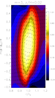
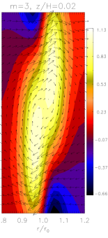
Figure 3.— Perturbed horizontal velocity field in the $(r,\phi)$ plane, for the locally isothermal disk with $h=0.07$ and $\mathcal{A}=1.25$ (left) and with $\mathcal{A}=1.6$ (right). The contours indicate relative density perturbation. The case with $\mathcal{A}=1.6$ displays a double-peak in density perturbation, which is explained in Li et al. (2000).

5.3. Vertical flow

We now examine vertical flow associated with the RWI. We focus on the co-rotation region since this is where relative density perturbations are largest and vortex-formation is expected.

Fig. 4 shows the perturbed vertical velocity field in the $(r,z)$ plane, at several azimuths. Since the largest contribution to $\delta v_{z}$ comes from the $l=2$ term in the expansion for $W$ (Eq. 32), the magnitude of $\delta v_{z}$ increases linearly with $z$.

Ahead and behind the vortex core, the flow just follows the anti-cyclonic motion, with radial variations in $\delta v_{z}$ being negligible. At $\phi=\phi_{0}$ there is also very little vertical motion for $z\lesssim 0.5H$, but there is upwards motion at $r=0.9,\,1.1$, i.e. the edge of the vortex (see Fig. 3). This can affect how dust particles are collected by RWI vortices.

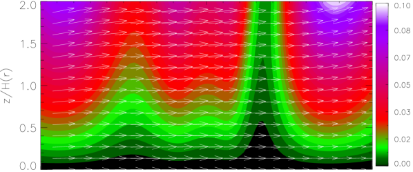
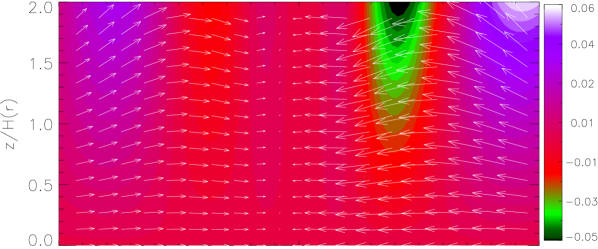
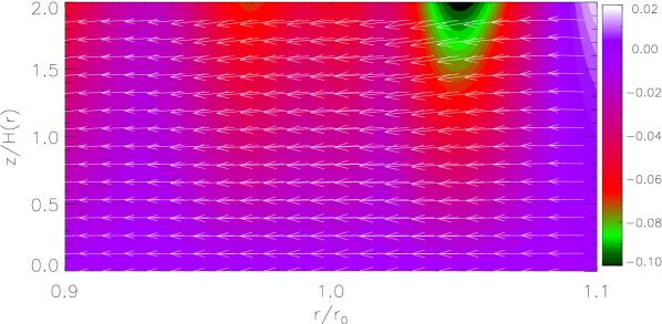
Figure 4.— Vertical velocity field (contours) for the $m=3$ mode in the locally isothermal disk with $h=0.07$, in the $(r,z)$ plane at azimuths $\theta\equiv m(\phi-\phi_{0})=0.2\pi$ (top), $0$ (middle) and $-0.2\pi$ (bottom). Arrows indicate the perturbed velocity field projected onto this plane.

For comparison, Fig. 5 shows the vertical flow for the $m=2$ mode. This flow is more two-dimensional than the fiducial case above. This is expected for decreasing $m$ (see, e.g. Papaloizou & Pringle, 1985; Goldreich et al., 1986). It also appears qualitatively different (e.g. downwards flow at $r=1.1$ instead of upwards as see for $m=3$). We typically find locally isothermal disks to display a wider range of flow patterns around co-rotation than polytropic disks presented later, which show generic patterns.

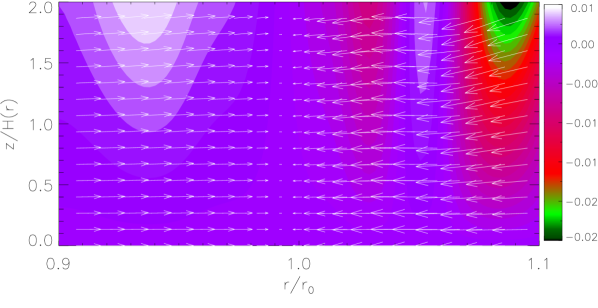
Figure 5.— Vertical velocity field (contours) for the $m=2$ mode in the locally isothermal disk with $h=0.07$. The slice is taken at the azimuth $\phi=\phi_{0}$. This figure is to be compared with the middle plot in Fig. 4. Arrows indicate the perturbed velocity field projected onto this plane.

Finally, Fig. 6 shows the perturbed vertical velocity in the $(\phi,z)$ plane at $r=r_{0}$. Vertical motion is upwards ahead of an anti-cyclonic vortex and downwards behind it. The vertical velocity can be comparable to the perturbed azimuthal velocity, so the perturbed flow is fully three-dimensional in this plane. However, the vortex center $(r_{0},\phi_{0})$ remains in vertical hydrostatic balance. This is not the case for polytropic disks.

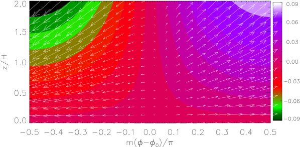
Figure 6.— Vertical velocity field (contours) for the $m=3$ mode in the locally isothermal disk with $h=0.07$, in the $(\phi,z)$ plane at the radius $r=r_{0}$. Arrows indicate the perturbed velocity field projected onto this plane.

5.4. Dependence of vertical flow on instability strength

We now assess how the three-dimensionality of the flow in the co-rotation region varies with instability strength. We examine ratio $\langle{|\delta v_{z}|}\rangle/\langle{|\delta v_{r}|}\rangle$ , where $\langle\cdot\rangle$ denotes averaging over $r\in[0.9,1.1]$ and $z\in[0,2H]$ at fixed azimuth $\phi=\phi_{0}$. In calculating this ratio, we ignore $W_{l>2}$ because the dominant contribution to $\delta v_{r}$ and $\delta v_{z}$ comes from $W_{0}$ and $W_{2}$ respectively. This ratio is large if there is significant vertical motion.

Results are shown in Fig. 7, where the bump amplitude $\mathcal{A}$ is increased at fixed $h=0.07$. Growth rates increase with $\mathcal{A}$, which is expected from previous works (Li et al., 2000), but the flow actually becomes less three-dimensional with increasing instability strength.

In the co-rotation region where $\bar{\sigma}\sim\mathrm{i}\gamma$, we expect from the linearized equation of motion that

$$|\delta v_{z}|\sim\frac{c_{s}^{2}}{H}\left|\frac{W_{2}}{\gamma}\mathcal{H}_{2}^{\prime}\right|.$$ (45)

$|\delta v_{z}|$ scales with $1/|\gamma|$, so that increasing growth rates contributes to decreasing $|\delta v_{z}|$. Thus, the flow in the co-rotation region does not necessarily become more three-dimensional with increasing $\mathcal{A}$.

It is clear from Fig. 7 that three-dimensionality decreases because of increasing $|\gamma|$ since $\langle{|W_{2}|}\rangle/\langle{|W_{0}|}\rangle$ varies weakly. We demonstrate this in Fig. 8, which shows that in the disk with $\mathcal{A}=1.6$ the flow is mainly horizontal. As in the fiducial case with $\mathcal{A}=1.25$, there is little motion at $r=r_{0}$.

Figure 7.— Average magnitude of vertical velocity (solid), in the co-rotation region of the RWI in the locally isothermal disk, as a function of bump amplitude $\mathcal{A}$ at fixed aspect-ratio $h$. Also shown are the normalized amplitude of $W_{2}$ in this region (dashed) and the growth rates (dotted).

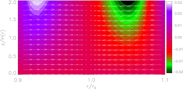
Figure 8.— Same as Fig. 4 but for a disk with $\mathcal{A}=1.6$. The slice is taken at $\phi=\phi_{0}$.

Fig. 7—8 shows that in the locally isothermal disk, more unstable modes are also more two-dimensional (in the co-rotation region). $|W_{2}|$ remains a small fraction of $|W_{0}|$ and $|\delta v_{z}|$ is largely affected by $|\gamma|$.

However, $|\gamma|$ can be obtained by just solving the 2D problem. Thus, we could have anticipated the trend of $|\delta v_{z}|$ in Fig. 7 based on only 2D calculations, with the assumption that changes in $|W_{2}|$ are less significant than the increase in $|\gamma|$. The above explicit calculation confirm this, suggesting we interpret the RWI as predominantly a 2D instability and that three-dimensional effects on the RWI are small (for low $m$). We further illustrate these points with polytropic disks below.

6. Results: polytropic disks

Our fiducial polytropic disk has polytropic index $n=1.5$. In the absence of a bump, a surface density profile $\propto r^{-1/2}$ gives a constant aspect-ratio ($H\propto r$). The bump parameters are set to $\mathcal{A}=1.4$ and $h=0.14$. Recall that for polytropic disks, $H$ is the disk thickness and $h$ is the aspect-ratio at $r_{0}$.

Although the surface density enhancement is relatively large, it corresponds to only $\simeq 9\%$ enhancement of the disk thickness at $r_{0}$. The background disk is shown in Fig. 9 in terms of the vortensity profile. The fiducial disk has a global vortensity gradient ($\eta\propto r^{-1}$ away from $r_{0}$), but it is the local minimum that drives instability. The epicycle frequency is such that $\mathrm{min}(\kappa^{2}/\Omega_{k}^{2})=0.47$.

Figure 9.— Background profile of the fiducial polytropic disk with $n=1.5,\,\mathcal{A}=1.4$ and $h=0.14$, in terms of the vortensity.

6.1. Solution examples

Eigenfrequencies for the fiducial case are shown in Table 2. The modes of interest are those with disturbance amplitudes largest near $r_{0}$, which were found to correspond to $m\leq 4$. These modes have effectively the same growth rates in 2D and 3D. This gives confidence that the RWI is an 2D instability. We will consider $m=3$ below in order to compare with locally isothermal disks. The $m=3$ growth rate is only slightly smaller than the most unstable $m=4$ mode. In co-rotation region, low $m$ modes are also insensitive to radial boundary conditions(Lin & Papaloizou, 2011a).

Table 2Eigenfrequencies in the $n=1.5$ polytropic disk

$m$	$-\sigma_{R}/(m\Omega_{0})$	$-10^{2}\gamma/\Omega_{0}$
1	0.9930 (0.9930)	4.4900 (4.4907)
2	0.9934 (0.9934)	8.2793 (8.2867)
3	0.9941 (0.9941)	10.769 (10.793)
4	0.9947 (0.9946)	11.594 (11.591)
5	0.9952 (0.9945)	10.646 (10.861)
6	0.9954 (0.9950)	8.0092 (8.5802)

Note. — Values in brackets were obtained from the 2D problem.

Fig. 10 shows the $S_{l}$ functions for the $m=3$ case. These are similar to the locally isothermal disk (Fig. 2). We typically find the $l>0$ radial functions to have larger amplitudes (compared to $l=0$) in the polytropic disk than in locally isothermal disks. $S_{l>0}$ have small but non-zero amplitudes near co-rotation, and their amplitude in the wave-like regions are at most $\simeq 20\%$ of $|S_{0}(r_{0})|$.

Figure 10.— Radial functions $S_{l}$ for the $n=1.5$ fiducial polytropic disk. These are normalized by $|S_{0}(r_{0})|$. The $l>0$ modes have also been magnified in order to compare its radial structure with $S_{0}$.

In the wave-like region, $|S_{l>0}|$ can be comparable or larger than $|S_{0}|$. We found the solution in the wave regions more strongly affected by boundary conditions than in locally isothermal disks.

We remark that for $m=5,\,6$, $S_{0}$ no longer has largest disturbance amplitude around $r_{0}$, because radial confinement around co-rotation requires low $m$ (Lin & Papaloizou, 2011a), unless the vortensity minimum is very deep. At sufficiently large $m$ (which depends on parameters), the modes are dominated by the wave-like region (much like the $m=5$ mode in locally isothermal disks, see Fig. 2). Boundary conditions are likely to play a role here, but they are not the vortex-forming RWI modes of interest.

6.2. Vertical structure

We now examine the $m=3$ mode in more detail. The flow in the $(r,\phi)$ plane is similar to the locally isothermal disk. However, consistent with the previous section, vertical motion was found to be more prominent in the polytropic disk.

As before we focus on the region $r\in[0.9,1.1]$. Fig. 11 shows upwards vertical motion at the vortex core and is largest near $z=H$. The flow for $z/H\lesssim 0.5$ and/or away from $r_{0}$ is essentially horizontal. The converging flow pattern in Fig. 11 is consistent with $(r_{0},\phi_{0})$ being an over-density. At the vortex core, upwards motion makes sense since the midplane is reflecting. It also implies an increase in disk thickness at $(r_{0},\phi_{0})$.

The background polytropic disk becomes thicker at $r_{0}$ (i.e. $H$ varies on a local scale). Fluid moving into the vortex core finds itself in a region of larger vertical extent. Upwards motion enhances the disk thickness, consistent with enhanced pressure and with the RWI vortices being over-pressure regions.

In the locally isothermal disk, it is difficult to directly associate vertical motion with enhanced pressure as above, since the scale-height is prescribed to vary on a global scale and it remains unperturbed. Hence, vertical motion at $(r_{0},\phi_{0})$ was not seen in locally isothermal disks.

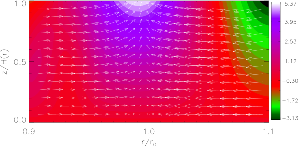
Figure 11.— Vertical velocity field for the $m=3$ mode in the $n=1.5$ fiducial polytropic disk. The slice is taken in the $(r,z)$ plane at the azimuth $\phi=\phi_{0}$. Arrows are the perturbed velocity field projected onto this plane.

We have also examined the vertical flow in the polytropic disk for other $m$ ($\leq 4$), but found similar flow structure. This is unlike the locally isothermal disk which can display a range of vertical flow pattern depending on $m$. (Fig. 4—5). This hints that there is a physical reason why polytropic disks tend to have positive vertical velocity at $r_{0}$. We return to this point later.

Lastly, Fig. 12 shows the vertical flow in the $(\phi,z)$ plane at $r=r_{0}$. The flow is similar to that in the locally isothermal disk (Fig. 6) except that the region $\phi\sim\phi_{0}$ is not in vertical hydrostatic equilibrium.

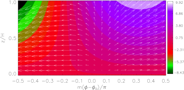
Figure 12.— Vertical velocity field for the $m=3$ mode in the $n=1.5$ fiducial polytropic disk. The slice is taken in the $(\phi,z)$ plane at radius $r=r_{0}$. Arrows are the perturbed velocity field projected onto this plane.

6.3. Effect of $h$ and $\mathcal{A}$

We measure the three-dimensionality of the flow in the co-rotation region in the same way as in §5.4, but here the averages are taken over the finite vertical extent of the disk.

Fig. 13—14 show results from calculations with variable $h$ (at fixed $\mathcal{A}=1.4$) and variable $\mathcal{A}$ (at fixed $h=0.14$), respectively. The range of growth rates are similar to the cases examined for the locally isothermal disk (see Fig. 7). $|\gamma|$ and $\langle{|X_{2}|}\rangle$ also behave similarly.

Figure 13.— Effect of $h$ on three-dimensionality of the co-rotation flow (solid). Also shown are the normalized amplitude of $S_{2}$ in this region (dashed) and the growth rates (dotted). The increase in growth rates with $h$ is expected because the RWI is driven by pressure forces (Li et al., 2000).

Figure 14.— Same as Fig. 13, but as a function of bump amplitude $\mathcal{A}$.

As in locally isothermal disks, Fig. 13—14 shows that the three-dimensionality of the flow decreases with instability strength, but less rapidly in polytropic disks. Overall, $\langle{|\delta v_{z}|}\rangle/\langle{|\delta v_{r}|}\rangle$ does not vary much, consistent with our findings that the vertical flow structure, such as Fig. 11— 12, to be generic. Such plots are qualitatively similar across the range of $h$ and $\mathcal{A}$ considered. The vertical flow at the vortex core is always upwards.

When the spatial average is taken over $r\in[0.98,1.02]$, we found $\langle{\delta v_{z}}\rangle/\langle{|\delta v_{r}|}\rangle$ maximizes at $h=0.16$ for fixed $\mathcal{A}$ and at $\mathcal{A}=1.6$ for fixed $h$. However, its values are of similar size: $\langle{\delta v_{z}}\rangle/\langle{|\delta v_{r}|}\rangle\simeq 0.44$—$0.65$ and $\langle{\delta v_{z}}\rangle/\langle{|\delta v_{r}|}\rangle\simeq 0.53$—$0.65$ for variable $h$ and $\mathcal{A}$, respectively. A reason for such insensitivity is that the above calculations have fixed polytropic index $n$, thereby fixing the fluid properties. Below, we show that varying $n$ affects the vertical flow.

6.4. Other polytropic indices

The polytropic index $n$ not only affects the magnitude of the bump in the background disk thickness but also the compressibility of the fluid. An isothermal fluid can be considered a polytrope with $n\to\infty$ and is highly compressible, while $n=0$ corresponds to an incompressible fluid. Thus increasing $n$ also increases compressibility.

For polytropic disks we identified vertical flow at the vortex core. Here, we focus on this region and take radial averages over $r\in[0.98,1.02]$. Fig. 15 show calculations for $n\in[1,2.4]$. As $n$ decreases, instability strength increases and the vertical flow at $r_{0}$ noticeably increases, so the motion becomes more three-dimensional. This is qualitatively different from varying $h$ or $\mathcal{A}$, where the vertical flow at the vortex core remain of similar size.

At the co-rotation radius, which is close to $r_{0}$, the vertical velocity is

$$|\delta v_{z}| \sim\left|\frac{S_{2}}{\gamma H_{0}}\mathcal{C}^{\lambda}_{2}{{}^{\prime}}\right|=\left|(4n^{2}-1)\frac{zS_{2}}{\gamma H_{0}^{2}}\right|.$$ (46)

$H_{0}$ is constant for fixed $h$. The factor $|(4n^{2}-1)/\gamma|$ decreases with decreasing $n$, which by itself would reduce the vertical velocity. Fig. 15 shows this is not the case. The increase in $|S_{2}|$ with decreasing $n$ overcomes this effect.

Figure 15.— Dependence of the vertical flow at the vortex core on the polytropic index $n$ (solid). The bump amplitude is fixed to $\mathcal{A}=1.4$ and $h=0.14$. Also shown are the growth rates (dotted) and amplitude of $S_{2}$ (dashed). The mode is $m=3$.

In Fig. 16 we compare the flow in the $(r,z)$ plane between $n=1$ and $n=2$. As previously remarked, the flows share the same qualitative feature: converging towards $r_{0}$ with upwards motion near $r_{0}$. However, for smaller $n$ (stronger instability), upwards motion is concentrated at $r_{0}$ whereas for larger $n$ (weaker instability) there is also upwards motion away from the vortex core. The latter was also seen for locally isothermal disks, consistent with larger $n$ being more compressible.

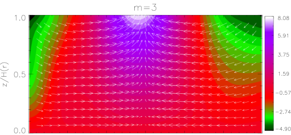
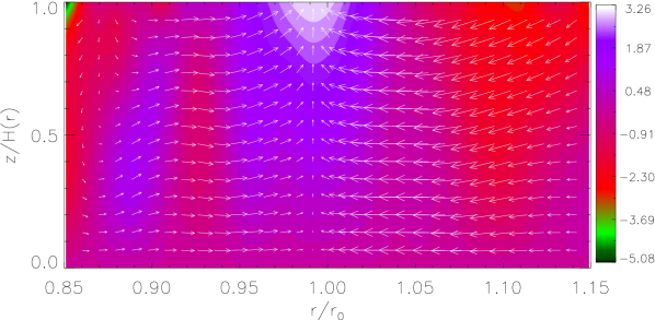
Figure 16.— Comparison between vertical velocity (contour) in a disk with polytropic index $n=1$ (top) and $n=2$ (bottom). Arrows indicate the velocity field projected onto this plane.

A larger vertical velocity at $r_{0}$ with decreasing $n$ is consistent with variable compressibility. First note that $|S_{2}|\ll|S_{0}|$ in $r\in[0.9,1.1]$ so the perturbed enthalpy, radial and azimuthal velocities are all dominated by $S_{0}$, which gives converging flow towards the vortex core where there is enhanced pressure or density. We may then ask what vertical motion at $r_{0}$ is compatible with this 2D perturbed flow, as implied by $S_{0}$?

At the vortex core $(r_{0},\phi_{0})$, the linearized continuity equation is approximately

$$\partial_{t}(\delta\rho/\rho)\sim-\nabla\cdot\delta\bm{v}-\delta v_{z}\partial_{z}\ln{\rho},$$

where the $\delta$ quantities are regarded as real. If the fluid is highly compressible (large $n$), then the density at the vortex core may increase with vertical motion playing no role. That is, the divergence term on the RHS dominates over the second ($\nabla\cdot\delta\bm{v}$ itself dominated by horizontal velocities).

However, if the fluid is made less compressible (decreasing $n$), so that $\nabla\cdot\delta\bm{v}$ is reduced in magnitude, then the fluid at $(r_{0},\phi_{0})$ should move upwards so that $-\delta v_{z}\partial_{z}\ln\rho>0$ contributes to increasing the density. For $n\ll 1$, the fluid becomes incompressible so that $\nabla\cdot\delta\bm{v}$ is negligible. Then the density can only increase by the fluid moving upwards, increasing the disk thickness and accommodating more material.

It is important to note that in the above argument, we deduced vertical motion by imposing the 2D solution in the three-dimensional disk. Effectively, we regarded $S_{0}$ is a source for $S_{2}$, and that $S_{2}$ has no back-reaction on $S_{0}$. This interpretation may not work for general disturbances, however. Here it is justified by the fact that $|S_{2}|\ll|S_{0}|$ from the numerical calculations. Calculations where the disk is truncated by setting $r_{i}=0.7,\,r_{o}=1.3$, thereby excluding the wave-like regions in $S_{l}$, show similar upwards motion. This indicates that $S_{0}$ induces $S_{2}$ locally.

7. Disks with $\kappa^{2}<0$

Meheut et al. (2010) performed the first nonlinear hydrodynamic simulations that showed evidence for the RWI in a 3D polytropic disk. Their fiducial calculation showed the development of a $m=1$ anti-cyclonic vortex which survived many orbits.

Indeed, the consideration of polytropic disks in this paper was originally inspired by these simulations, but it turns out that the disk model employed by Meheut et al. (2010) has a region where $\kappa^{2}<0$. Motivated by this feature, in this section we use Meheut et al. (2010)’s disk model to explore the 3D RWI when $\kappa_{0}^{2}<0$. We find that the RWI can be quite different to those described previously (where $\kappa^{2}>0$ everywhere).

It is straight forward to adapt our setups to models used by Meheut et al.. They considered a $n=1.5$ polytropic disk, occupying $r\in[r_{i},r_{o}]=[1,6]$, and specified the midplane density to be a power law ($\rho_{0}\propto r^{-1/2}$) with a Gaussian bump. Their bump in midplane density has the same functional form as that used for surface density in our models (Eq. 2), so $\mathcal{A}$ is now the bump amplitude in midplane density. The bump is located at $r_{0}=3$ with width $\Delta r=0.1r_{i}$. The calculations presented below employed $N_{r}=768$ grid points, on account of the larger disk compared to previous models.

We will consider the $m=1$ mode below. Calculations were done for $m\leq 6$, which gave similar growth rates when $\kappa_{0}^{2}<0$, but provided $\mathcal{A}$ is chosen to ensure $\kappa_{0}^{2}>0$, then higher $m$ modes become dominant (e.g., with $\mathcal{A}=1.15$, $m=5$ had the highest growth rate). The latter is qualitatively consistent with very recent numerical simulations (Meheut et al., 2012a, see also Appendix B.1).

When $\kappa_{0}^{2}>0$, we find similar flow structure to that described previously. Having applied the linear calculations to a different disk model and recovering similar results gives us confidence in the robustness of the RWI to develop 3D.

7.1. $m=1$ modes

In their fiducial setup, Meheut et al. adopted a bump amplitude of $\mathcal{A}=1.4$. This results in $\kappa^{2}=0$ at $r\simeq 0.99r_{0},\,1.01r_{0}$ and $\kappa^{2}_{0}<0$ (which is also reflected in their Fig. 9). The disk is therefore unstable to local axisymmetric perturbations (Chandrasekhar, 1961).

Interestingly, for $\mathcal{A}=1.4$ we found a $m=1$ mode with large growth rate, $|\gamma|=0.36\Omega_{0}$, almost twice the largest growth rates found previously. Below, we examine this solution along with a case with $\mathcal{A}=1.3$, which has $\kappa^{2}>0$ everywhere and growth rate $|\gamma|=0.05\Omega_{0}$.

Despite $\mathcal{A}$ being similar, the $m=1$ growth rate for $\mathcal{A}=1.3$ is much smaller than that for $\mathcal{A}=1.4$. For $\mathcal{A}=1.3$ we did not find other $m=1$ modes with growth rates similar to the $m=1$ mode in $\mathcal{A}=1.4$. Furthermore, for $\mathcal{A}=1.4$ the quantity $D=\kappa^{2}-\bar{\sigma}^{2}$ almost vanishes near $r_{0}$:

$$\mathrm{min}(|D|/\Omega_{k}^{2})=4\times 10^{-3},$$

which occurs at $r=1.002r_{0}$. For $\mathcal{A}=1.3$, the value above is $0.14$.

Fig. 17 compares the $S_{l}$ functions for the cases above. While the double-peak in $S_{0}$ for $\mathcal{A}=1.3$ was also found in previous sections and also by Li et al. (2000), it is absent in $\mathcal{A}=1.4$. The dominant 3D mode is $S_{2}$, but it is significantly larger in $\mathcal{A}=1.4$ than in $\mathcal{A}=1.3$. This indicates the vertical flow will also be qualitatively different.

Figure 17.— Radial functions $S_{l}$ for the polytropic disk model with a bump in midplane density of amplitude $\mathcal{A}=1.4$ (top, Meheut et al.’s fiducial setup) and with a bump amplitude of $\mathcal{A}=1.3$ (bottom). For $\mathcal{A}=1.4$, $\kappa_{0}^{2}<0$.

Fig. 18 shows the flow pattern at $\phi=\phi_{0}$ for $\mathcal{A}=1.4$. This result is very different from that for $\mathcal{A}=1.3$, which share the same features as our previous setups with $\kappa^{2}>0$ (e.g. Fig. 11). Note that while the $S_{l}$ behave smoothly across $r_{0}$ (Fig. 17), numerical evaluation of $\delta v_{r}$ involves a division by $D$, which is very small near $r_{0}$ for $\mathcal{A}=1.4$. Thus, horizontal velocities may be subject to numerical artifacts at $r_{0}$. Despite this, the direction of radial flow, being inwards for $r<r_{0}$ and outwards for $r>r_{0}$ with a sharp transition at $r_{0}$, was also found in Meheut et al. (2010, their Fig. 11).

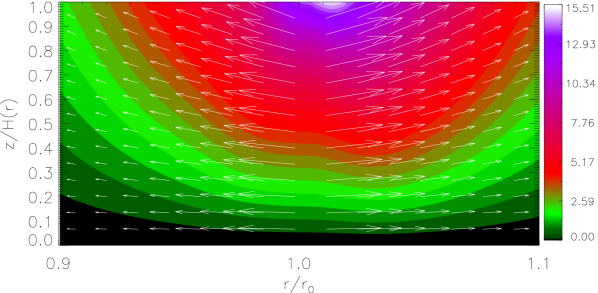
Figure 18.— Vertical velocity field for a $m=1$ mode in Meheut et al. (2010)’s disk model with $\mathcal{A}=1.4$, which results in in $\kappa^{2}<0$ at $r_{0}$ and $D\to 0$ there as well. The arrows are the perturbed velocity field projected onto this plane. This result is qualitatively different to modes with $\kappa^{2}>0$ (see figures in §6).

Neither $\mathcal{A}$ produced vertical flow consistent with that in Meheut et al. (2010) where strong downwards flow at $r_{0}$ were identified with rolls excited on either side. By contrast the linear solutions have upwards motion and there is no vortical motion in the $(r,z)$ plane.

Despite using the same disk models, several factors may have contributed to the discrepancy between the linear calculation above and Meheut et al.’s simulation. These include the treatment of the vertical domain, nonlinearities (H. Meheut, private communication) and interaction with other $m$ modes in the simulation which cannot be treated in linear theory.

There may also be numerical issues in our linear calculation because of $\kappa^{2}\leq 0$. The RWI is associated with the term $\propto(1/\bar{\sigma})\partial_{r}(\rho_{0}\Omega/D)$ and its disturbance is localized about $r_{0}$. This term is $\propto 1/\kappa^{2}$, which diverges when $\kappa^{2}\to 0$ near $r_{0}$. Also because $\kappa^{2}_{0}<0$, it allows $D\to 0$ at co-rotation as well. We have performed calculations with lower spatial resolution, so that numerically $\kappa^{2}$ and $D$ have larger deviations from zero, but we found similar eigenfrequencies and flow patterns to the case shown above. We will further comment on RWI modes with $\kappa_{0}^{2}<0$ in §8.3.

8. Summary and discussion

In this paper, we have examined the linear stability of three-dimensional, vertically stratified and radially structured disks. Our calculations are 3D analogs of those presented by Li et al. (2000), in which the Rossby wave instability was studied in razor-thin disks. In order to simplify the problem, we assumed the perturbed hydrodynamic quantities have vertical dependence that can be decomposed into Hermite or Gegenbauer polynomials. Our conclusions therefore apply to such perturbations only.

Our numerical calculations confirm the RWI persists in 3D. For ease of discussion below, we denote the full linear solution schematically as

$$X=Y(r)+\Delta Y(r,z),$$

where $Y$ is the $z$-independent part of the solution and $\Delta Y$ is the part that also depends on $z$.

8.1. Validity of 2D

We find the RWI growth rate $|\gamma|$ can be accurately determined from the 2D problem alone. In other words, instability is associated with $Y(r)$. In the region of interest — the vortensity minimum — where vortex-formation is expected, we find $|\Delta Y|\ll|Y|$ so that enthalpy, radial velocity and azimuthal velocity perturbations have essentially no $z$-dependence.

In fact, weak $z$-dependence is expected from earlier studies of accretion tori. For slender tori, Papaloizou & Pringle (1985) demonstrated the existence of low $m$ unstable modes with weak $z$-dependence. Goldreich et al. (1986) also justified the use of height-averaged equations for calculating modes in narrow tori, for which vertical hydrostatic equilibrium was assumed. Although we considered radially extended disks, their results should apply here because the low $m$ RWI modes, relevant to vortex-formation, have largest disturbance associated with a narrow region about the density bump. More recently, Umurhan (2010) reproduced the RWI in approximate three-dimensional disk models, in which horizontal velocities have no vertical dependence. Our numerical results are therefore supported by analytic studies above.

The 2D solution, $Y$, imply anti-cyclonic motion associated with over-densities, thus we expect the RWI will lead to columnar vortices in 3D. The survival of vortices in 3D is then an important issue because they may be subject to instabilities (Lesur & Papaloizou, 2009, 2010). On the other hand, if there is a continuous source of vortensity extremum, such as disk-planet interaction, then vortex-formation via the RWI could be maintained.

8.2. Vertical motion

Although $|\Delta Y|$ is small in the co-rotation region, it is nevertheless non-zero. This implies vertical motion growing on dynamical time-scales, making the flow in the co-rotation region three-dimensional. We found the nature of the vertical flow is affected by the equation of state.

In polytropic disks the vortex core $(r_{0},\phi_{0})$ always involve upwards motion. For fixed polytropic index $n$, there is limited variation in the magnitude of vertical flow with respect to instability strength. However, if the fluid is made less compressible by lowering $n$, then vertical motion at the vortex core increases.

This result motivates us to interpret vertical motion around co-rotation as a perturbation to the 2D solution (Goldreich et al., 1986). Recall that $Y$ is the solution to the vertically integrated system. It signifies non-axisymmetric enhancements in surface density at the bump radius. This characteristic feature is unchanged by the addition of $\Delta Y$ to the 2D solution. We then ask how should the disk respond in the vertical direction.

The polytropic disk thickness is directly related to the surface density (Eq. 12). Enhancement of the surface density therefore imply enhancement in disk thickness, so fluid at $(r_{0},\phi_{0})$ moves upwards. If we look in the $(\phi,z)$ plane at $r_{0}$, the disk thickness becomes non-axisymmetric. This has already been observed in nonlinear simulations (Meheut et al., 2011a, b). In these newer simulations, the authors indeed find upwards motion in anti-cyclonic vortices.

Note that the polytropic disk thickness becomes less sensitive to surface density as $n$ is increased (Eq. 12). For $n\to\infty$ the disk thickness is independent of surface density and there is no need for fluid to move vertically in order to achieve a surface density increase. In this case there is no preference for vertical velocity of a particular sign at $(r_{0},\phi_{0})$. Since the fluid behaves isothermally as $n\to\infty$, the above is consistent with our observation that locally isothermal disks have little vertical motion right at the vortex core. In Appendix B.2 we consider a polytropic disk calculation with $n=8$ to check for consistency.

8.3. RWI with $\kappa^{2}<0$

We briefly examined the linear 3D RWI in disk where $\kappa^{2}$ becomes negative at the density bump. This was inspired by the 3D RWI simulations presented in Meheut et al. (2010), where the disk model had $\kappa_{0}^{2}<0$. In this setup we found a $m=1$ linear mode with large growth rate and qualitatively different to modes in disks with $\kappa^{2}>0$ everywhere. In neither case did we reproduce the vertical flow seen in Meheut et al. (2010), namely downwards flow at the vortex center.

Most discussions of non-axisymmetric disk instabilities have assumed $\kappa^{2}>0$ everywhere, including Lovelace et al. (1999)’s original description of the RWI, so that Rayleigh’s criterion for stability against local axisymmetric perturbations is satisfied.

The RWI has been shown to exist for $\kappa_{0}^{2}<0$ but its properties appear different to those in disks with $\kappa_{0}^{2}>0$. For example, Li et al. (2000)’s linear calculations indicate a non-smooth change in growth rate as $\kappa_{0}^{2}$ becomes negative (the ‘HGB’ case in their Fig. 9). In nonlinear 2D simulations by Li et al. (2001), the RWI also evolves differently depending on whether the growth rate is low ($|\gamma|\sim 0.1\Omega_{0}$ and $\kappa_{0}^{2}>0$) or high ($|\gamma|\sim 0.3\Omega_{0}$ and $\kappa_{0}^{2}<0$). Note the latter case has $|\gamma|$ close to that found in our calculation. We therefore expect the RWI to differ in 3D depending on $\operatorname{sgn}(\kappa_{0}^{2})$. This is apparent by comparing our results with $\kappa_{0}^{2}>0$ to those with $\kappa_{0}^{2}<0$.

Thus, while Meheut et al. (2010) is the first demonstration of the 3D RWI, it should be kept in mind that the disk model has $\kappa_{0}^{2}<0$. An understanding of such modes in 3D is of theoretical interest, but it is unclear whether or not protoplanetary disks will develop sufficiently large pressure gradients to render $\kappa^{2}<0$ (Yang & Menou, 2010).

8.4. Outstanding issues

The main goal of our study is to demonstrate the linear RWI in 3D and to identify the nature of associated three-dimensional flow structure around co-rotation. However, our study is subject to several caveats which should be clarified in future work.

8.4.1 Baroclinic effects

One issue is that our locally isothermal basic states are not in true equilibrium, because we approximated the rotation profile to be $z$-independent (Eq. 8). Initializing a full hydrodynamic simulation this way might boost radial velocities because of the inexact radial momentum balance. In order for the angular velocity to be strictly independent of $z$, we must set $H\propto r^{3/2}$, which is the globally isothermal disk already considered by Meheut et al. (2012b). We do not expect this to make a difference from our disks with $H\propto r$, because the RWI is driven by local variations in disk structure and its disturbance is radially confined. We check this in Appendix B.2.

Another justification is that for a thin, smooth disk ($\mathcal{A}=1$) with $H=hr$, the angular velocity is

$$\Omega(r,z)=\Omega_{k}\left[1-\frac{h^{2}}{2}\left(\alpha+2+\frac{z^{2}}{2H^{2}}\right)\right]$$ (47)

(Tanaka et al., 2002). The difference in angular speed between the gas at the midplane and gas at $z$ is then

$$\Delta\Omega\equiv|\Omega(r,z)-\Omega(r,0)|=h^{2}\left(\frac{z^{2}}{4H^{2}}\right)\Omega_{k}$$ (48)

(a radial density bump does not contribute to this difference). Since the gas is contained within a few scale-heights, we have $\Delta\Omega/\Omega_{k}=O(h^{2})$. Because $h\ll 1$, vertical shear should be unimportant if the dynamics of interest operate on much faster time-scales, as can be the case for the RWI with growth rates $\sim h\Omega_{k}$. That is, the vortical perturbation grows much faster than it is sheared apart by $\Delta\Omega$. We have begun preliminary nonlinear simulations which confirms vortex formation via the RWI in a locally isothermal 3D disk with constant aspect-ratio (Lin 2012, in preparation).

Knobloch & Spruit (1986) have pointed out the possibility of baroclinic instability in the case of $\Omega=\Omega(r,z)$, when there are radial variations in temperature on the scale of local scale-heights. This condition is not met in our locally isothermal disk models because the sound-speed varies on a global scale. In more realistic disk models, one might expect that a density bump also involves local temperature variations. Baroclinic effects may then become important. On the other hand, the RWI may also be enhanced because of local temperature gradients (Li et al., 2000). Having $\Omega=\Omega(r,z)$ means solving the linearized equations as a PDE eigenvalue problem, which is not simple.

8.4.2 Boundary effects

We have restricted our attention to the co-rotation region because this is where vortex-formation eventually takes place. Distant radial boundaries do not affect the dynamics in this region significantly (as checked numerically). However, it is clear that far away from co-rotation, three-dimensional effects become increasingly important. This is seen in the polytropic disk as $|\Delta Y|\sim|Y|$ towards the disk boundaries (Fig. 10). Disturbances associated with the RWI are therefore three-dimensional beyond the Lindblad resonances. In order to study these regions, more physically realistic radial boundary conditions are needed.

Around co-rotation the RWI is a global disturbance in $z$, so the upper disk boundary conditions could be important. The use of orthogonal polynomials means we simply impose a regularity condition at the upper disk boundary (§4). This method of solution does not allow us to explore the effect of other vertical boundary conditions. Again, such a study involves a PDE eigenvalue problem, but can reveal to what extent the dominance of the 2D solutions found here are influenced by the specific decompositions employed. This will be the subject of a follow up paper.

Nevertheless, we can make some speculations based on results here. The vanishing density at the polytropic disk surface is likely to provide a reflective upper boundary. This effect may be important. It might reduce the growth of the RWI if it remains predominantly a 2D disturbance, because the 2D solution alters the surface density, which is directly related to the disk thickness for a polytrope, but the disk thickness cannot change.

Appendix A Explicit expressions for the linear operators

A.1. Locally isothermal disks with constant aspect-ratio

For locally isothermal disks with $H=hr$ with $h$ being a constant and $\Omega$ taken to be a function of radius only, the operators governing the linear problem are given by

$$A_{l}= \left[\frac{2mr\Omega}{\bar{\sigma}}\frac{d}{dr}\ln{\left(\frac{c_{s}^{2}\Sigma\Omega}{D}\right)}-\left(m^{2}+\frac{r^{2}D}{c_{s}^{2}}\right)+\frac{lD}{\bar{\sigma}^{2}h^{2}}-lr\frac{d}{dr}\ln{\left(\frac{c_{s}^{2}\Sigma}{D}\right)}-l(2l-1)+\frac{4m\Omega l}{\bar{\sigma}}\right]$$

$$+r^{2}\frac{d}{dr}\left[\ln{\left(\frac{rc_{s}^{2}\Sigma}{D}\right)}\right]\frac{d}{dr}+r^{2}\frac{d^{2}}{dr^{2}},$$ (A1)

$$B_{l}= -\left[(l-2)-\frac{2m\Omega}{\bar{\sigma}}\right]+r\frac{d}{dr},$$ (A2)

$$C_{l}= -(l+1)(l+2)\left[r\frac{d}{dr}\ln{\left(\frac{c_{s}^{2}\Sigma}{D}\right)}+l-\frac{2m\Omega}{\bar{\sigma}}\right]-r(l+1)(l+2)\frac{d}{dr}.$$ (A3)

We have expressed the operators in terms of surface density $\Sigma$ so the above may be seen to be equivalent to Eq. 21 in Tanaka et al. (2002) when their parameter $\mu=d\ln{H}/d\ln{r}$ is set to unity.

These equations are approximate because we ignored terms proportional to $\partial_{z}\Omega$ in the governing PDE from which Eq. A1—A3 are derived. These terms are non-vanishing for exact equilibrium if the sound-speed varies with radius, but for a thin disk $\partial_{z}\Omega\propto h^{2}\ll 1$ so we expect them to be small. It is worth neglecting them in favor of the one-dimensional operators above, which are much simpler. Tanaka et al. (2002) gives a more general equation for the linear problem which includes $\partial_{z}\Omega$. Their Eq. 11 shows that $\partial_{z}\Omega$ contributes to the coefficient of $\partial_{z}W$ as

$$\frac{\partial W}{\partial z}\left[\frac{z}{H^{2}}+\frac{m}{\bar{\sigma}}\frac{\partial\Omega}{\partial z}\right]=\frac{z}{H^{2}}\frac{\partial W}{\partial z}\left[1-\frac{mh^{2}q\Omega_{k}}{\bar{\sigma}}\right],$$ (A4)

where $\partial_{z}\Omega$ is evaluated using Tanaka et al.’s Eq. 4 and $q\equiv-d\ln{c_{s}}/d\ln{r}=0.5$ for disks with constant aspect-ratio (equivalent to Eq. 48 in §8.4.1). Near co-rotation the magnitude of the second to first term is

$$\left|mh^{2}q\frac{\Omega_{k}}{\bar{\sigma}}\right|\sim\frac{mh^{2}q}{|\gamma/\Omega_{k}|}.$$ (A5)

For the fiducial case in §5, $m=3,\,h=0.07$ and $|\gamma/\Omega_{k}|\simeq 0.057$, this ratio is 0.13. We typically find $|\gamma/\Omega_{k}|=O(h)$, so the second term is a factor $mhq\ll 1$ smaller than the first for low $m$ modes. Neglecting it (to arrive at Eq. A1—A3) is a self-consistent treatment.

A.2. Polytropic disks

For polytropic disks, we find it most convenient to express the linear operators as

$$A_{0}= -\mathcal{V}^{(1)}+\frac{(2\lambda+1)}{2(\lambda+1)}\left[\mathcal{V}^{(2)}-\mathcal{V}^{(4)}+\mathcal{V}^{(6)}-\mathcal{V}^{(7)}+\mathcal{V}^{(8)}\right],$$ (A6)

$$A_{l>0}= -\mathcal{V}^{(1)}+\frac{1}{2(l+\lambda+1)(l+\lambda-1)}\left\{\left(l^{2}+2\lambda l+2\lambda^{2}-\lambda-1\right)\left[\mathcal{V}^{(2)}+\mathcal{V}^{(6)}+\mathcal{V}^{(8)}\right]\right.$$

$$\phantom{-\mathcal{V}^{(1)}+\frac{1}{2(l+\lambda+1)(l+\lambda-1)h}}+l(l+2\lambda)\left[\lambda\mathcal{V}^{(3)}-\left(l^{2}+2\lambda l-1\right)\mathcal{V}^{(5)}\right]$$

$$\phantom{-\mathcal{V}^{(1)}+\frac{1}{2(l+\lambda+1)(l+\lambda-1)h}}-\left[(\lambda+1)l^{2}+2\lambda(\lambda+1)l+2\lambda^{2}-\lambda-1\right]\mathcal{V}^{(4)}$$

$$\phantom{-\mathcal{V}^{(1)}+\frac{1}{2(l+\lambda+1)(l+\lambda-1)h}}\left.-(l^{2}+2\lambda l+\lambda-1)(2\lambda+1)\mathcal{V}^{(7)}\right\}-l(l+2\lambda)\mathcal{V}^{(9)},$$ (A7)

$$B_{l}= -\frac{l(l-1)}{4(l+\lambda-2)(l+\lambda-1)}\left\{\mathcal{V}^{(2)}+(l-2)\mathcal{V}^{(3)}+(l+2\lambda-1)\left[\mathcal{V}^{(4)}+(l-2)\mathcal{V}^{(5)}\right]\right.$$

$$\phantom{-\frac{l(l-1)}{4(l+\lambda-2)(l+\lambda-1)}h}\left.+\mathcal{V}^{(6)}+(2\lambda+1)\mathcal{V}^{(7)}+\mathcal{V}^{(8)}\right\},$$ (A8)

$$C_{l}= \frac{(l+2\lambda+1)(l+2\lambda)}{4(l+\lambda+1)(l+\lambda+2)}\left\{-\mathcal{V}^{(2)}+(l+2\lambda+2)\mathcal{V}^{(3)}+(l+1)\left[\mathcal{V}^{(4)}-(l+2\lambda+2)\mathcal{V}^{(5)}\right]\right.$$

$$\phantom{\frac{(l+2\lambda+1)(l+2\lambda)}{4(l+\lambda+1)(l+\lambda+2)}h}\left.-\mathcal{V}^{(6)}-(2\lambda+1)\mathcal{V}^{(7)}-\mathcal{V}^{(8)}\right\},$$ (A9)

where

$$\mathcal{V}^{(1)} =\frac{nD\rho_{0}^{-1/n}r^{2}}{K(1+n)},\quad\mathcal{V}^{(2)}=r^{2}\left\{\frac{d}{dr}\left[\ln{\left(\frac{\rho_{0}r}{D}\right)}\right]\frac{d}{dr}+\frac{d^{2}}{dr^{2}}\right\},\quad\mathcal{V}^{(3)}=-r^{2}\left\{\frac{H^{\prime}}{H}\frac{d}{dr}\left[\ln{\left(\frac{\rho_{0}r}{D}\right)}\right]+\left(\frac{H^{\prime}}{H}\right)^{\prime}+\frac{H^{\prime}}{H}\frac{d}{dr}\right\},$$

$$\mathcal{V}^{(4)} =-r^{2}\frac{H^{\prime}}{H}\frac{d}{dr},\quad\mathcal{V}^{(5)}=r^{2}\left(\frac{H^{\prime}}{H}\right)^{2},\quad\mathcal{V}^{(6)}=\frac{2mr\Omega}{\bar{\sigma}}\frac{d}{dr}\left[\ln{\left(\frac{\rho_{0}\Omega}{D}\right)}\right],$$

$$\mathcal{V}^{(7)} =-\frac{2mr\Omega}{\bar{\sigma}}\left(\frac{H^{\prime}}{H}\right),\quad\mathcal{V}^{(8)}=-m^{2},\quad\mathcal{V}^{(9)}=-\frac{r^{2}D}{\bar{\sigma}^{2}H^{2}}.$$ (A10)

We have used the midplane density $\rho_{0}$, but it is straight forward to express the above in terms of $\Sigma$ using the relation $\Sigma=\rho_{0}H(r)I_{n}$. The form of the operators above are appropriate for numerical computations in the range of polytropic indices considered in this paper ($n\geq 1$ or $\lambda\geq 0.5$). Numerical issues may arise for smaller indices because of the $(l+\lambda-2)^{-1}$ factor in $B_{l}$. For example, if $\lambda=0$ ($n=0.5$) and $l=2$ this factor diverges. However, for $n=0.5$ it is more natural to use Chebyshev polynomials of the first kind ($T_{l}$) for expansion in $\hat{z}$. We have performed calculations with $n=0.5$ using $T_{l}$, and found similar results to those presented here.

Appendix B Supplementary calculations

B.1. Improved simulations

During the finishing stages of this paper, Meheut et al. (2012a) published new simulations of the 3D RWI with improved numerical resolution. This simulation developed a $m=5$ mode with growth rate $|\gamma|=0.17\Omega_{0}$, with upwards motion at anti-cyclonic vortex centers and downwards motion at cyclonic vortex centers, which are consistent with our fiducial polytropic disks (§6).

We were able to find a $m=5$ linear mode provided the bump amplitude $\mathcal{A}$ in the midplane density was chosen to ensure $\kappa^{2}>0$. Using $\mathcal{A}=1.7$, we find $|\gamma|=0.18\Omega_{0}$ for $m=5$. This mode is shown in Fig. 19. Note that $S_{0}$ is still localized about $r_{0}$, despite the higher $m$ than those considered in our fiducial calculations (which gave more global disturbances). This is because here the vortensity minimum is deep, with $\mathrm{min}(\kappa^{2}/\Omega_{k}^{2})\simeq 0.1$, so even high $m$ modes can be localized. The vertical flow at the vortex core is upwards, as found previously.

Meheut et al. (2012a) actually employed $\mathcal{A}=2$, giving $\kappa_{0}^{2}\simeq-0.2\Omega_{k}^{2}$, for which we were unable to find a linear mode with similar growth rate as their simulation. As $\kappa_{0}^{2}$ is more negative in their new simulation than in Meheut et al. (2010), one possibility is that an axisymmetric disturbance develops early on, rendering $\kappa^{2}\gtrsim 0$ then the usual RWI follows. For $\mathcal{A}=1.7$ we find linear growth rates peak at $m=8$ with $|\gamma|=0.21\Omega_{0}$, but this is only marginally larger than $m=5$. Differences in the linear and nonlinear calculations, such as the treatment of vertical boundaries, may then account for observation of $m=5$ in the simulations.

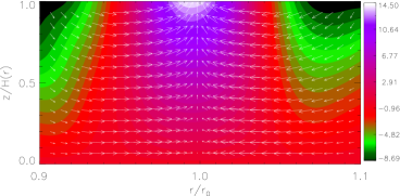
Figure 19.— A linear $m=5$ mode found in Meheut et al. (2012a)’s $n=1.5$ polytropic disk model, but with a smaller bump amplitude than their simulation. Left: radial eigenfunctions $S_{l}$ normalized by $|S_{0}(r_{0})|$. Right: vertical flow structure.

B.2. Consistency check

We describe calculations to check the consistency between locally isothermal and polytropic disks and against the globally isothermal disk presented in Meheut et al. (2012b).

Noting that an isothermal disk is a special case of a polytropic disk in the limit of large $n$, we performed a polytropic disk calculation with $n=8,\,\mathcal{A}=2.0,\,h=0.2$. Fig. 20 show that in this case vertical motion is much smaller than the horizontal flow in the co-rotation region, compared to smaller values of $n$ discussed in §6.4. This is consistent with our typical results for locally isothermal disks were the vertical velocity vanishes at the vortex core.

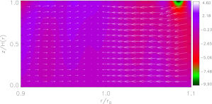
Figure 20.— A $m=3$ mode in the standard $n=8$ polytropic disk (growth rate $|\gamma|=0.055\Omega_{0}$). Contours of the real vertical velocity perturbation are shown. Arrows are the perturbed velocity field projected onto this plane. This figure is similar to locally isothermal disks in that there is very little vertical velocity near the vortex core, and is unlike polytropic disks with smaller $n$ (e.g Fig. 16, which shows significant upwards motion near $r=r_{0}$).

Meheut et al. (2012b) solved the linear problem for globally isothermal disks. Their basic state with $\Omega=\Omega(r)$ satisfy exact radial momentum balance but adopting such a profile for locally isothermal disks is only approximate. We have performed a locally isothermal calculation with the same parameters as Meheut et al. (2012b). The result is shown in Fig. 21. It shares the same vertical flow implied by Meheut et al. (2012b)’s Fig. 3d around a maximum in the (real) density perturbation: $\delta v_{z}>0$ near $r=1.1$, $\delta v_{z}<0$ near $r=0.9$ and $\delta v_{z}\sim 0$ at $r=r_{0}$. This suggests that a node in the vertical velocity at the vortex core is a generic feature for linear RWI modes in isothermal disks. A global temperature profile does not affect the 3D RWI significantly.

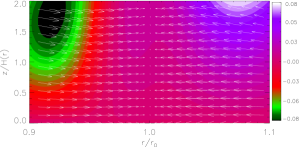
Figure 21.— A linear mode in the locally isothermal disk with the same parameter values as the Meheut et al. (2012b)’s globally isothermal disk ($m=4,\,h=0.1,$ other parameters are the same as our fiducial case in §5). Contours of the real vertical velocity perturbation is shown. Arrows are the perturbed velocity field projected onto this plane. The growth rate $|\gamma|=0.20\Omega_{0}$ is similar to Meheut et al.. The vertical flow is also consistent with their Fig. 3d, namely the vertical velocity vanishes near $r=r_{0}$.

References

- Abramowitz & Stegun (1965) Abramowitz, M., & Stegun, I. A. 1965, Handbook of mathematical functions with formulas, graphs, and mathematical tables, ed. Abramowitz, M. & Stegun, I. A.
- Armitage (2011) Armitage, P. J. 2011, ARA&A, 49, 195
- Balbus & Hawley (1991) Balbus, S. A., & Hawley, J. F. 1991, ApJ, 376, 214
- Barge & Sommeria (1995) Barge, P., & Sommeria, J. 1995, A&A, 295, L1
- Chandrasekhar (1961) Chandrasekhar, S. 1961, Hydrodynamic and hydromagnetic stability, ed. Chandrasekhar, S.
- Crespe et al. (2011) Crespe, E., Gonzalez, J.-F., & Arena, S. E. 2011, in SF2A-2011: Proceedings of the Annual meeting of the French Society of Astronomy and Astrophysics, ed. G. Alecian, K. Belkacem, R. Samadi, & D. Valls-Gabaud, 469–473
- de Val-Borro et al. (2007) de Val-Borro, M., Artymowicz, P., D’Angelo, G., & Peplinski, A. 2007, A&A, 471, 1043
- Dong et al. (2011) Dong, R., Rafikov, R. R., & Stone, J. M. 2011, ApJ, 741, 57
- Gammie (1996) Gammie, C. F. 1996, ApJ, 457, 355
- Goldreich et al. (1986) Goldreich, P., Goodman, J., & Narayan, R. 1986, MNRAS, 221, 339
- Goldreich & Tremaine (1979) Goldreich, P., & Tremaine, S. 1979, ApJ, 233, 857
- Goldreich & Tremaine (1980) —. 1980, ApJ, 241, 425
- Knobloch & Spruit (1986) Knobloch, E., & Spruit, H. C. 1986, A&A, 166, 359
- Koller et al. (2003) Koller, J., Li, H., & Lin, D. N. C. 2003, ApJ, 596, L91
- Lesur & Papaloizou (2009) Lesur, G., & Papaloizou, J. C. B. 2009, A&A, 498, 1
- Lesur & Papaloizou (2010) —. 2010, A&A, 513, A60
- Li et al. (2001) Li, H., Colgate, S. A., Wendroff, B., & Liska, R. 2001, ApJ, 551, 874
- Li et al. (2000) Li, H., Finn, J. M., Lovelace, R. V. E., & Colgate, S. A. 2000, ApJ, 533, 1023
- Li et al. (2005) Li, H., Li, S., Koller, J., Wendroff, B. B., Liska, R., Orban, C. M., Liang, E. P. T., & Lin, D. N. C. 2005, ApJ, 624, 1003
- Li et al. (2009) Li, H., Lubow, S. H., Li, S., & Lin, D. N. C. 2009, ApJ, 690, L52
- Li et al. (2003) Li, L.-X., Goodman, J., & Narayan, R. 2003, ApJ, 593, 980
- Lin & Papaloizou (1986) Lin, D. N. C., & Papaloizou, J. 1986, ApJ, 309, 846
- Lin & Papaloizou (2010) Lin, M.-K., & Papaloizou, J. C. B. 2010, MNRAS, 405, 1473
- Lin & Papaloizou (2011a) —. 2011a, MNRAS, 415, 1426
- Lin & Papaloizou (2011b) —. 2011b, MNRAS, 415, 1445
- Lovelace et al. (1999) Lovelace, R. V. E., Li, H., Colgate, S. A., & Nelson, A. F. 1999, ApJ, 513, 805
- Lyra et al. (2008) Lyra, W., Johansen, A., Klahr, H., & Piskunov, N. 2008, A&A, 491, L41
- Lyra et al. (2009) Lyra, W., Johansen, A., Zsom, A., Klahr, H., & Piskunov, N. 2009, A&A, 497, 869
- Meheut et al. (2010) Meheut, H., Casse, F., Varniere, P., & Tagger, M. 2010, A&A, 516, A31
- Meheut et al. (2012a) Meheut, H., Keppens, R., Casse, F., & Benz, W. 2012a, ArXiv e-prints
- Meheut et al. (2011a) Meheut, H., Varniere, P., & Benz, W. 2011a, in EPSC-DPS Joint Meeting 2011, held 2-7 October 2011 in Nantes, France, 1054
- Meheut et al. (2011b) Meheut, H., Varniere, P., Casse, F., & Tagger, M. 2011b, in EPSC-DPS Joint Meeting 2011, held 2-7 October 2011 in Nantes, France, 1059
- Meheut et al. (2012b) Meheut, H., Yu, C., & Lai, D. 2012b, MNRAS, 2748
- Muto et al. (2010) Muto, T., Suzuki, T. K., & Inutsuka, S.-i. 2010, ApJ, 724, 448
- Narayan et al. (1987) Narayan, R., Goldreich, P., & Goodman, J. 1987, MNRAS, 228, 1
- Okazaki & Kato (1985) Okazaki, A. T., & Kato, S. 1985, PASJ, 37, 683
- Ou et al. (2007) Ou, S., Ji, J., Liu, L., & Peng, X. 2007, ApJ, 667, 1220
- Papaloizou & Pringle (1984) Papaloizou, J. C. B., & Pringle, J. E. 1984, MNRAS, 208, 721
- Papaloizou & Pringle (1985) —. 1985, MNRAS, 213, 799
- Papaloizou & Pringle (1987) —. 1987, MNRAS, 225, 267
- Regály et al. (2012) Regály, Z., Juhász, A., Sándor, Z., & Dullemond, C. P. 2012, MNRAS, 419, 1701
- Takeuchi & Miyama (1998) Takeuchi, T., & Miyama, S. M. 1998, PASJ, 50, 141
- Tanaka et al. (2002) Tanaka, H., Takeuchi, T., & Ward, W. R. 2002, ApJ, 565, 1257
- Terquem (2008) Terquem, C. E. J. M. L. J. 2008, ApJ, 689, 532
- Umurhan (2008) Umurhan, O. M. 2008, A&A, 489, 953
- Umurhan (2010) —. 2010, A&A, 521, A25
- Umurhan (2012) —. 2012, ArXiv e-prints
- Varnière & Tagger (2006) Varnière, P., & Tagger, M. 2006, A&A, 446, L13
- Yang & Menou (2010) Yang, C.-C., & Menou, K. 2010, MNRAS, 402, 2436
- Yu & Li (2009) Yu, C., & Li, H. 2009, ApJ, 702, 75
- Yu et al. (2010) Yu, C., Li, H., Li, S., Lubow, S. H., & Lin, D. N. C. 2010, ApJ, 712, 198
- Zhang & Lai (2006) Zhang, H., & Lai, D. 2006, MNRAS, 368, 917