The S-Star Cluster at the Center of the Milky Way

Sagittarius A*, the super-massive black hole at the center of the Milky Way, is surrounded by a small cluster of high velocity stars, known as the S-stars. We aim to constrain the amount and nature of stellar and dark mass associated with the cluster in the immediate vicinity of Sagittarius A*. We use near-infrared imaging to determine the $K_{\mathrm{s}}$-band luminosity function of the S-star cluster members, and the distribution of the diffuse background emission and the stellar number density counts around the central black hole. This allows us to determine the stellar light and mass contribution expected from the faint members of the cluster. We then use post-Newtonian N-body techniques to investigate the effect of stellar perturbations on the motion of S2, as a means of detecting the number and masses of the perturbers. We find that the stellar mass derived from the $K_{\mathrm{s}}$-band luminosity extrapolation is much smaller than the amount of mass that might be present considering the uncertainties in the orbital motion of the star S2. Also the amount of light from the fainter S-cluster members is below the amount of residual light at the position of the S-star cluster after removing the bright cluster members. If the distribution of stars and stellar remnants is strongly enough peaked near Sagittarius A*, observed changes in the orbital elements of S2 can be used to constrain both their masses and numbers. Based on simulations of the cluster of high velocity stars we find that at a wavelength of 2.2 $\mu$m close to the confusion level for 8 m class telescopes blend stars will occur (preferentially near the position of Sagittarius A*) that last for typically 3 years before they dissolve due to proper motions.

1 Introduction

Using 8–10 m class telescopes, equipped with adaptive optics (AO) systems, at near-infrared (NIR) wavelengths has allowed us to identify and study the closest stars in the vicinity of the super-massive black hole (SMBH) at the center of our Milky Way. These stars, referred to as the S-star cluster, are located within the innermost arcsecond, orbiting the SMBH, Sagittarius A*(Sgr A*), on highly eccentric and inclined orbits. Up till now, the trajectories of about 20 stars have been precisely determined using NIR imaging and spectroscopy (Gillessen et al. 2009a, b). This orbital information is used to determine the mass of the SMBH and can in principle be used to detect relativistic effects and/or the mass distribution of the central stellar cluster (Rubilar & Eckart 2001; Zucker et al. 2006; Mouawad et al. 2005; Gillessen et al. 2009a).

One of the brightest members of that cluster is the star S2. It has the shortest observed orbital period of $\sim$15.9 years, and was the star used to precisely determine the enclosed dark mass, and infer the existence of a $\sim$4 million solar mass SMBH, in our own Galactic center (GC; Schödel et al. 2002; Ghez et al. 2003). The first spectroscopic studies of S2, by Ghez et al. (2003) and later Eisenhauer et al. (2005), revealed its rotational velocity to be that of an O8-B0 young dwarf, with a mass of 15 $M_{\odot}$ and an age of less than $10^{6}$ yrs. Later, Martins et al. (2008) confined the spectral type of S2 to be a B0–2.5 V main-sequence star with a zero-age main-sequence (ZAMS) mass of 19.5 $M_{\odot}$. The fact that S2, along with most of the S-stars, is classified as typical solar neighborhood B2–9 V stars, indicates that they are young, with ages between 6–400 Myr (Eisenhauer et al. 2005). The combination of their age and the proximity to Sgr A* presents a challenge to star formation theories. It is still unclear how the S-stars were formed. Being generated locally requires that their formation must have occurred through non-standard processes, like formation in at least one gaseous disk (Löckmann et al. 2009) or via an eccentricity instability of stellar disks around SMBHs (Madigan et al. 2009). Alternatively, if they formed outside the central star cluster, about 0.3 parsec core radius (e.g. Buchholz et al. 2009; Schödel et al. 2007), there are several models that describe how they may have been brought in (e.g. Hansen & Milosavljević 2003; Kim et al. 2004; Levin et al. 2005; Fujii et al. 2009, 2010; Merritt et al. 2009; Gould & Quillen 2003; Perets et al. 2007, 2009). For a detailed description of these processes see Perets & Gualandris (2010).

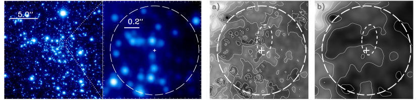
Figure 1: Left: $17.5^{\prime\prime}\times 17.5^{\prime\prime}$ NACO $K_{\mathrm{s}}$-band mosaic of the central cluster zoomed in to the inner 1–$2^{\prime\prime}$ region around Sgr A*. The inner region is indicated by a dashed (white) circle. Right: a) Map of the diffuse background light within a circle of $0.69^{\prime\prime}$ radius centered on the position of Sgr A*, shown here as a cross at the center. The projected orbit of the star S2 is over-plotted as an ellipse. b) The same map smoothed by convolution with a Gaussian beam of FWHM $=6$ pixels. The contours levels are at 95%, 90%, 80%, 70%, 60%, 50%, 40%, 30%, 20% and 10% of the maximum flux value for each image.

Stellar dynamics predict the formation of a cusp of stars at the center of a relaxed stellar cluster around a SMBH. This is manifested by an increase in the three dimensional stellar density of old stars and remnants towards the center with power-law slopes of 1.5 to 1.75 (Bahcall & Wolf 1976; Murphy et al. 1991; Lightman & Shapiro 1977; Alexander & Hopman 2009).

The steep power-law slope of 1.75 is reached in the case of a spherically symmetric single mass stellar distribution in equilibrium. For a cluster with differing mass composition, mass segregation sets in, where the more massive stars sink towards the center, while the less massive ones remain less concentrated. This leads to the shallow density distribution of 1.5 (Bahcall & Wolf 1977). Later numerical simulations and analytical models confirmed these results (Freitag et al. 2006; Preto & Amaro-Seoane 2010; Hopman & Alexander 2006b). These steep density distributions were expected for the central cluster considering its age, which is comparable to the estimates of the two-body relaxation-time of 1–20 Gyr for the central parsec (Alexander 2005; Merritt 2010; Kocsis & Tremaine 2011). However, observations of the projected stellar number density, which can be related to the three dimensional density distribution, revealed that the cluster’s radial profile can be fitted by two power-law slopes. The slope for the whole cluster outside a radius of $\sim 6^{\prime\prime}$ (corresponding to 0.22 parsec) was found to be as steep as $1.8\pm 0.1$, while inside the break radius the slope was shallower than expected and reached an exponent of $1.3\pm 0.1$ (Genzel et al. 2003; Schödel et al. 2007). These findings motivated the need to derive the density profiles of the distinct stellar populations, given that recent star formation (6 Myr, Paumard et al. 2006) at the GC gave birth to a large number of high-mass young stars that would be too young to reach an equilibrium state. Using adaptive optics and intermediate-band spectrophotometry Buchholz et al. (2009) found the distribution of late-type stars (K giants and later) to be very flat and even showing a decline towards the Center (for a radius of less that $6^{\prime\prime}$), while the early-type stars (B2 main-sequence and earlier) follow a steeper profile. Similar results were obtained later by Do et al. (2009) and Bartko et al. (2010).

These surprising findings required new models to explain the depletion in the number of late-type giants in the central few arcseconds around the SMBH. Such attempts involved Smooth Particle Hydrodynamics (SPH) and Monte Carlo simulations which tried to account for the under density of giants by means of collisions with other stars and stellar remnants (Dale et al. 2009; Freitag 2008). Another explanation could be the disturbance of the cusp of stars after experiencing a minor merger event or an in-spiraling of an intermediate-mass black hole, which then would lead to deviations from equilibrium; hence causing a shallower power-law profile of the cusp (Baumgardt et al. 2006). Merritt (2010) explains the observations by the evolution of a parsec-scale initial core model.

Mouawad et al. (2005) presented the first efforts to determine the amount of extended mass in the vicinity of the SMBH allowing for non-Keplerian orbits. Using positional and radial velocity data of the star S2, and leaving the position of Sgr A* as a free input parameter, they provide, for the first time, a rigid upper limit on the presence of a possible extended dark mass component around Sgr A*. Considering only the fraction of the cusp mass $M_{\mathrm{S2_{apo}}}$ that may be within the apo-center of the S2 orbit, Mouawad et al. (2005) find $M_{\mathrm{S2_{apo}}}/(M_{\mathrm{SMBH}}+M_{\mathrm{S2_{apo}}})\leq 0.05$ as an upper limit. This number is consistent with more recent investigations of the problem (Gillessen et al. 2009b). Due to mass segregation, a large extended mass in the immediate vicinity of Sgr A*, if present, is unlikely to be dominated in mass of sub-solar mass constituents. It could well be explained by a cluster of high $M/L$ stellar remnants, which may form a stable configuration.

From the observational point of view, several attempts have been made recently to tackle the missing cusp problem. Sazonov et al. (2011) proposed that the detected $1^{\prime\prime}$ sized thermal X-ray emission close to Sgr A* (Baganoff et al. 2001, 2003) can be explained by the tidal spin-ups of several thousand late-type main-sequence stars (MS). They use the Chandra X-ray data to infer an upper limit on the density of these low-mass main-sequence stars. Furthermore, using Hubble Space Telescope (HST) data, Yusef-Zadeh et al. (2012) derived a stellar mass profile, from the diffuse light profile in the region $<1^{\prime\prime}$ around Sgr A*, and by that they explained the diffuse light to be dominated by a cusp of faint K0 dwarfs.

Up to now, the true distribution of the Nuclear Star Cluster, especially the S-stars, is yet to be determined. No investigations have confirmed or ruled out the existence of a cusp of relaxed stars and stellar remnants around Sgr A*, as predicted by theory. An excellent dataset to investigate the stellar content of the central arcsecond around Sgr A* is the NIR $K_{\mathrm{s}}$-band (2.2 $\mu$m) data (see Figure 1) we used in (Sabha et al. 2010, hereafter NS10). In that case we subtracted the stellar light contribution to the flux density measured at the position of Sgr A*. The aim of this work is then to analyze the resulting image of the diffuse NIR background emission close to the SMBH. This emission is believed to trace the accumulative light of unresolved stars (Schödel et al. 2007; Yusef-Zadeh et al. 2012). We explain the background light by extrapolating the $K_{\mathrm{s}}$-band luminosity function (KLF) of the innermost (1–2^′′, corresponding to 0.05 parsecs for a distance of 8 kpc to the GC) members of the S-star cluster to fainter $K_{\mathrm{s}}$-magnitudes. We compare the cumulative light and mass of these fainter stars to the limits imposed by observations. We then extend our analysis to explore the possible nature of this background light by testing its effect on the observed orbit of the star S2. Furthermore, we simulate the distribution of the unresolved faint stars ($K_{\mathrm{s}}>18$) and their combined light to produce line-of-sight clusterings that have a compact, close to stellar, appearance.

The paper is structured as follows: Section 2 deals with a brief description of the observation and data reduction. We describe in Section 3 the method used (§ 3.1–§ 3.3) and discuss the different observational limits (§ 3.4) employed to test our analysis. Exploring the possible contributors to the dark mass within the orbit of S2 is done in Section 4. In Section 5 we give the results obtained by simulating the distribution of faint stars and the possibility of producing line of sight clusterings that look like compact stellar objects. We summarize and discuss the implications of our results in Section 6. We adopt throughout this paper $\Sigma(R)\propto R^{-\Gamma}$ as the definition for the projected density distribution of the background light , with $R$ being the projected radius and $\Gamma$ the corresponding power-law index.

2 Observations and data reduction

The observations and data reduction have been described in NS10. In summary: The near-infrared (NIR) observations have been conducted at the Very Large Telescope (VLT) of the European Southern Observatory (ESO) on Paranal, Chile. The data were obtained with YEPUN, using the adaptive optics (AO) module NAOS and the NIR camera/spectrometer CONICA (briefly “NACO”). The data were taken in the $K_{\mathrm{s}}$-band (2.2 $\mu$m) on the night of 23 September 2004, and is one of the best available where Sgr A* is in a quiet state. The flux densities were measured by aperture photometry with circular apertures of 66 mas radius. They were corrected for extinction, using $A_{K_{\mathrm{s}}}=2.46$ derived for the inner arcsecond from Schödel et al. (2010). Possible uncertainties in the extinction of a few tenths of a magnitude do not influence the general results obtained in this paper. The flux density calibration was carried out using zero points for the corresponding camera setup and a comparison to known $K_{\mathrm{s}}$-band flux densities of IRS16C, IRS16NE (Schödel et al. 2010, from;Blum et al. 1996, also) and to a number of the S-stars (Witzel et al. 2012).

3 The central few tenths of parsecs

In NS10 we gave a stringent upper limit on the emission from the central black hole in the presence of the surrounding S-star cluster. For that purpose, three independent methods were used to remove or strongly suppress the flux density contributions of these stars, in the central $\sim 2^{\prime\prime}$, in order to measure the flux density at the position of Sgr A*. All three methods provided comparable results, and allowed a clear determination of the stellar light background at the center of the Milky Way, against which Sgr A* has to be detected. The three methods, linear extraction of the extended flux density, automatic and iterative point spread function (PSF) subtraction were carried out assuming that the extracted PSF in the central few arcseconds of the image is uniform. Investigations of larger images (e.g. Buchholz et al. 2009) show that on scales of a few arcseconds the constant PSF assumption is valid, while for fields $\geq 10^{\prime\prime}$ the PSF variations have to be taken into account.

Figure 2 is a map of the 51 stars adopted from the list in Table 3 of NS10. The stars are plotted relative to the position of Sgr A*. The surface number density of these detected stars, within a radial distance of about $0.5^{\prime\prime}$ from Sgr A*, is $68\pm 8$ arcsec^-2, with the uncertainty corresponding to the square-root of that value. This value agrees with the central number density of $60\pm 10$ arcsec^-2 given by Do et al. (2009). Extrapolating the KLF allows us to test if the observed diffuse light across the central S-star cluster, or the amount of unaccounted dark mass, can be explained by stars.

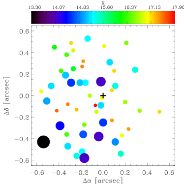
Figure 2: Map of the 51 stars listed in Table 3 from NS10. The color of each star indicates its $K_{\mathrm{s}}$-magnitude. The size of each symbol is proportional to the flux of the corresponding star. The position of Sgr A* is indicated as a cross at the center.

3.1 KLF of the S-star cluster

Figure 3 shows the KLF histogram derived for the stars detected in the central field, (Figure 2). We improve the KLF derivation by choosing a fixed number of bins that allows for about 10 sources per bin while providing a sufficient number of points to allow for a clear linear fit. The Red Clump (RC)/Horizontal Branch (HB) stars, around $K_{\mathrm{s}}\approx 14.5$, are in one bin, so the RC/HB bump is visible there (Schödel et al. 2007). For estimating the uncertainty, we randomized the start of the first bin in an interval between $K_{\mathrm{s}}=13.0$ to $14.2$ and repeated the histogram calculation $10^{5}$ times. The number of sources in each bin was then determined by taking the average of all iterations and the uncertainties were subsequently derived from the standard deviation. We derive a least-square linear slope of $d\log(N)/d(K_{\mathrm{s}})=\alpha=0.18\pm 0.07$, which compares well with the KLF slope of $0.3\pm 0.1$ derived in NS10 and also with the KLF slope of $0.21\pm 0.02$ found for the inner field ($R<6^{\prime\prime}$) by Buchholz et al. (2009).

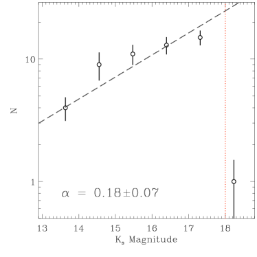
Figure 3: KLF histogram of the stars detected in the central field, derived from the 23 September 2004 data. The dashed line indicates the linear fit of the KLF slope of $\alpha=0.18\pm 0.07$. The vertical dotted line (red) represents the current detection limit for faint $K_{\mathrm{s}}$-magnitudes.

For the magnitudes up to $K_{\mathrm{s}}=17.50$ within the central $0.69^{\prime\prime}$ radius, we detect no significant deviation from a straight power-law. This implies that the completeness is high and can be compared to the $\sim$70% value derived for mag${}_{K}=17$ by Schödel et al. (2007) where the authors introduced artificial stars into their NIR image and attempted re-detecting them. However, for $K_{\mathrm{s}}=17.50$ to $18.25$ the stellar counts drop quickly to about $20\%$ of the value expected from the straight power-law line; hence the last $K_{\mathrm{s}}$-bin is excluded from the linear fit.

Maíz Apellániz & Úbeda (2005) propose an alternative way of binning when dealing with stellar luminosity and initial mass functions (IMF). Their method is based on choosing variable sized bins with a constant number of stars in each bin. They find that variable sized binning introduces bias-free estimations that are independent from the number of stars per bin. Their method is applicable to small samples of stars. We apply their method to our KLF calculation and get $d(\log(N)/\delta K_{\mathrm{s}})/d(K_{\mathrm{s}})=0.12\pm 0.09$, consistent with our fixed sized binning method.

3.2 The diffuse NIR background

The methods we used in NS10 to correct for the flux density contribution of the stars in the central $2^{\prime\prime}$ have revealed a faint extended emission around Sgr A* (NS10 Figures 3b, 4b and 5). We detected $\sim 1.3$ mJy (obtained by correcting the $\sim 2$ mJy we quote in NS10 for the $A_{K_{\mathrm{s}}}=2.46$ we use here) at the center of the S-star cluster. With a radius of $1^{\prime\prime}$ (about twice the FWHM of the S-star cluster) for the Point Spread Function (PSF) used for the subtraction, we showed that a misplacement of the PSF for about only five stars, located within one FWHM of Sgr A*, would contribute significantly to the measured flux at the center. For a median brightness of about 1.3 mJy for these stars, a 1 pixel $\sim 13$ mas positional shift of each of these stars towards Sgr A* would be required to explain all the detected $\sim 1.3$ mJy at the center i.e. 0.26 mJy from each star. In Sabha et al. (2011) we showed that a displacement larger than a few tenths of a pixel would result in a clear and identifiable characteristic plus/minus pattern in the residual flux distribution along the shift direction. For a maximum positional uncertainty of 1 pixel, we showed that the independent shifts of the five stars can be approximated by a single star experiencing five shifts in a random walk pattern. This resulted in calculating a total maximum contribution of 0.26 mJy from all the five stars to the center, which translates to about 20–30% of the flux density. Thus, more than two thirds of the extended emission detected towards Sgr A* could be due to faint stars, at or beyond the completeness limit reached in the KLF, and associated with the $\sim 0.5$–$1^{\prime\prime}$ diameter S-star cluster.

The diffuse background emission we detected (see Figure 1a) could be compared to the projected distribution of stars $\Sigma(R)\propto R^{-\Gamma}$, with $R$ being the projected radius. We found that the distribution of the azimuthally averaged residual diffuse background emission, centered on the position of Sgr A*, not to be uniform but in fact decreases gently as a function of radius (see Figure 7 in NS10) with a power-law index $\Gamma_{\mathrm{diffuse}}=0.20\pm 0.05$. In this investigation we re-calculate the azimuthally averaged background light from the iterative PSF subtracted image alone. The azimuthally averaged background light is plotted as a function of projected radius from Sgr A* in Figure 4. In this new calculation we find the power-law index to have a value of $\Gamma_{\mathrm{diffuse}}=0.14\pm 0.07$. Both results are consistent with recent investigations concerning the distribution of number density counts of the stellar populations in the central arcseconds, derived from imaging VLT and Keck data. For the central few arcseconds Buchholz et al. (2009), Do et al. (2009) and Bartko et al. (2010) find a $\Gamma\sim 1.5\pm 0.2$ for the young stars, but an even shallower distribution for the late-type (old) stars with $\Gamma\sim 0.2\pm 0.1$. A detailed discussion concerning the different populations and their distribution is given in Genzel et al. (2003); Schödel et al. (2007); Buchholz et al. (2009); Do et al. (2009) and Bartko et al. (2010).

The small value we obtain for the projected diffuse light exponent $\Gamma_{\mathrm{diffuse}}$ and the high degree of completeness reached around $K_{\mathrm{s}}=17.5$, makes this data set well suited for analyzing the diffuse background light. Especially in investigating the role of much fainter stars, beyond the completeness limit, in the observed power-law behavior of the background.

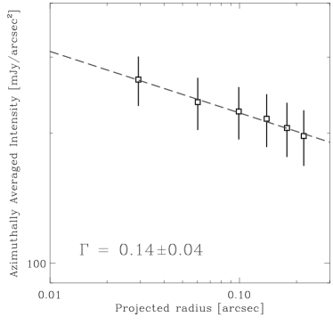
Figure 4: Azimuthal average of the diffuse background emission as derived from manual PSF subtracted 23 September 2004 image. The squares (mean flux and $1\sigma$ uncertainty per pixel) have been calculated in annuli of 39.8 mas (3 pixels) width. The black dashed line marks a fit to the data points with an exponential decrease of 0.14.

3.3 Extrapolating the KLF of the S-star cluster

Motivated by the power-law behavior of the diffuse background emission and assuming that the drop in the KLF counts at magnitude $\sim 18$ is caused only by the fact that we have reached the detection limit, we extrapolate the KLF to fainter magnitudes in order to investigate how these faint stars contribute to the background light. The true shape of the luminosity function for $K_{\mathrm{s}}$-magnitudes below the completeness limit of $\sim 17.5$ has yet to be determined. Investigations into the IMF of the S-cluster have shown that it can be fitted with a standard Salpeter/Kroupa IMF of $dN/dm\propto m^{-2.3}$ and continuous star formation histories with moderate ages (below 60 Myr, Bartko et al. 2010). Here, we estimate an upper limit on the stellar light by assuming that the KLF exhibits the same behavior observed for brighter magnitudes without suffering a break in the slope toward the fainter end.

We use the KLF slope we obtained for the innermost central region, $0.18\pm 0.07$ (Figure 3) and extrapolate it over five magnitudes bins to $K_{\mathrm{s}}\sim 25$. The $K_{\mathrm{s}}$-magnitude bins between 18–25 (translating to stellar masses in the range of $\sim$ 1.68 to 0.34 $M_{\odot}$) correspond to the brightness of the expected main-sequence stars (luminosity class V) which are likely to be present in the central cluster. However, we assume that due to mass segregation effects in the Galactic nucleus (Bahcall & Wolf 1976; Alexander 2005), driven by dynamical friction (Chandrasekhar 1943) between stars, the heavier objects sink towards the center while the lighter objects move out. Their volume density will be significantly reduced and they may even be expelled from the very center. Freitag et al. (2006) show that the main-sequence stars begin to be expelled outward by the cusp of stellar-mass black holes (SBH) after a few Gyrs, just shorter than the presumed age of the stellar cluster at about 10 Gyrs. While the reservoir of lower mass stars may be replenished by the most recent - possibly still ongoing - star formation episode about 6 million years ago (Paumard et al. 2006), we assume that stars well below our low mass limit of $\sim$ 0.34 $M_{\odot}$ with $K_{\mathrm{s}}$-band brightnesses around $K_{\mathrm{s}}=25$ are affected by depletion.

Figure 5 shows the KLF slope of $\alpha=0.18$ and the upper limit imposed by the uncertainty in the fit ($\alpha=0.25$) plotted as dashed and dash-dotted lines, respectively. The extrapolated $K_{\mathrm{s}}$-bins are shown as hollow circles. We adopt a Monte Carlo approach for calculating the number of stars $N$ from the KLF, taking into account the uncertainty in the slope. After $10^{5}$ trials we find as a result for each bin, the median number $N$ and median deviation $dN$.

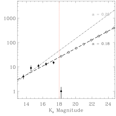
Figure 5: Extrapolation of the KLF power-law fit. The KLF slope of $\alpha=0.18$ and the upper limit imposed by the uncertainty in the fit ($\alpha=0.25$) are plotted as dashed and dash-dotted lines, respectively. The black filled circles represent the data while the hollow circles represent new points based on the extrapolated KLF slope. The approximate location of the detection limit is indicated by the vertical dotted/red line.

Using the extrapolated $K_{\mathrm{s}}$-magnitudes, the corresponding flux densities are calculated using the following relation

$$f_{\mathrm{new\ star}}=f_{\mathrm{S2}}\times 10^{-0.4\leavevmode\nobreak\ (K_{\mathrm{new\ star}}-K_{\mathrm{S2}})}\leavevmode\nobreak\ ,$$ (1)

where $f_{\mathrm{new\ star}}$ and $K_{\mathrm{new\ star}}$ are the flux density and $K_{\mathrm{s}}$-magnitude for each new star in the extrapolation. The flux and magnitude for the star S2 were adopted from NS10, Table 3, and corrected for the extinction value we use here (see § 2). The new values are $f_{\mathrm{S2}}=14.73$ mJy and $K_{\mathrm{S2}}=14.1$. The accumulative flux density for each $K_{\mathrm{s}}$-bin $f_{\mathrm{bin}}$ is obtained via

$$f_{\mathrm{bin}}=f_{\mathrm{new\ star}}\times N_{\mathrm{new\ star}}.$$ (2)

The number of stars per bin $N_{\mathrm{new\ star}}$ is randomly picked from the interval between $[N_{\mathrm{new\ star}}-dN_{\mathrm{new\ star}}]$ and $[N_{\mathrm{new\ star}}+dN_{\mathrm{new\ star}}]$. In $10^{5}$ trials the accumulative flux per bin and its uncertainty are determined as the median and median deviation of the randomly drawn fluxes $f_{\mathrm{bin}}$. We then add up all the accumulative flux densities for all the new $K_{\mathrm{s}}$-band bins and obtain the integrated brightness of the extrapolated part of the S-star cluster,

$$F_{\mathrm{Extra\ Stars}}=\sum_{K_{\mathrm{s}}\simeq 18}^{25}f_{\mathrm{bin}}=(25.72\pm 14.31)\quad\mathrm{mJy}.$$ (3)

We assume that the faint, undetectable stars follow the distribution of the azimuthally averaged background light, as shown in Figure 4. Thus, the light from the faint stars that we introduced in the $0.69^{\prime\prime}$ radius region can be compared to the measured background light from our data for the same region. This is achieved by using the total flux density $F_{\mathrm{Extra\ Stars}}$ to derive the peak light density ($I_{\mathrm{Extra\ Stars}}$) that would be measured inside one resolution element of $0.033^{\prime\prime}$ radius centered on the position of Sgr A*, using the following relation:

$$F_{\mathrm{Extra\ Stars}} = \int{f(r,\phi)rdrd\phi}$$ (4)

$$= 2\pi I_{\mathrm{Extra\ Stars}}\int_{0.033^{{}^{\prime\prime}}}^{0.690^{{}^{\prime\prime}}}{r^{1-\Gamma}dr},$$

with $\Gamma=\Gamma_{\mathrm{diffuse}}=0.14$ (see § 3.2). The peak light density for the extra stars is then $I_{\mathrm{Extra\ Stars}}=(15.24\pm 8.48)$ mJy arcsec^-2. To compare the light caused by the extra stars with the measured background emission, we plot the stellar light density caused by our new stars with the azimuthally averaged measured light density of the background (Figure 6). For illustration purposes we normalize the observed peak stellar light to the measured background value within the central resolution element, $I_{\mathrm{Background}}=(254.30\pm 58.45)$ mJy arcsec^-2. It is clear that the peak light introduced by the new faint stars, as calculated from the extrapolation of the $0.18\pm 0.07$ KLF slope, is very small and below that of the background. The dotted line (black circles) represents the background light while the dashed line (blue squares) corresponds to the extra stellar light. The upper limit of the extrapolated extra stellar light contribution is presented as a dashed line with no symbols. The figure shows that the upper limit of the extrapolated light contribution of the S-star cluster is lower than $15\%$ of the measured background light.

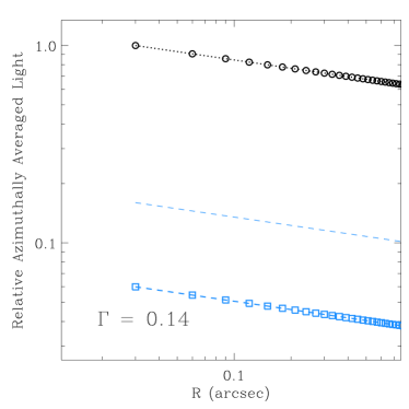
Figure 6: Relative azimuthally averaged light density, for the background light taken from the observations and the extra stellar light calculated from the extrapolation, plotted as a function of distance from Sgr A*. They are represented by a dotted line with circles (black) and dashed lines with squares (blue), respectively. The stellar light density is normalized to the peak light density of the background at the central resolution element. The upper limit of the extrapolated extra stellar light is shown as the blue dashed line with no symbols.

3.4 Observational limits on the stellar light and mass

Our analysis shows that if there was a population of very faint stars, following the extrapolated $K_{\mathrm{s}}$-band luminosity function and central cluster profile obtained for the brighter stellar population (less than $K_{\mathrm{s}}=18$), the additional stellar light and mass lie well below the limits given by observational data. See following sections and Figures 7 and 8.

3.4.1 Limits on the stellar light

Following the previous calculations and the result displayed in Figure 6, we perform our analysis for a range of KLF slopes in order to test if the observed background light can be solely obtained by the emission of faint stars. The range of KLF slopes we use is based on the values and uncertainty estimates of the following published KLF slopes for the central $2^{\prime\prime}$: $0.13\pm 0.02$ (Buchholz et al. 2009, early-type stars), $0.27\pm 0.03$ (Buchholz et al. 2009, late-type stars), $0.21\pm 0.02$ (Buchholz et al. 2009, all stars) and $0.30\pm 0.1$ (NS10), in addition to the improved newly fitted slope of the KLF in this work $0.18\pm 0.07$.

We extrapolate each KLF slope to a $K_{\mathrm{s}}$-magnitude of $\simeq 25$. The peak light density ($I_{\mathrm{Extra\ Stars}}$) is calculated using Equation (4). The peak light density of the extra stars is plotted for the extrapolated KLF slopes in the range of 0.11 to 0.40 in Figure 7 . The limit imposed by the peak light density of the measured background light (Figure 1) is plotted as a horizontal dashed line (blue). In addition, the KLF slopes derived in this work and by NS10 and Buchholz et al. (2009) are plotted as purple, yellow and green data points, respectively. Figure 7 clearly shows that almost all of the KLF slopes result in a peak light density below the observed limit, except for very high slopes $>0.37$ which are not in agreement with the observations.

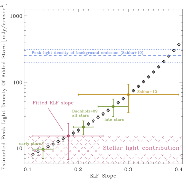
Figure 7: Estimated peak light density from stars derived from for different KLF slopes. Slopes of Buchholz et al. (2009) (for different stellar populations) are shown in green, NS10 in yellow and the KLF slope derived here, in § 3.1, in purple. A limit imposed by the measured peak light density from the measured background light is plotted as a horizontal dashed line (blue).

3.4.2 Limits on the stellar mass

Using the same range of KLF slopes, we estimate the mass that would be introduced to the central region as a result of the KLF extrapolation. We obtain the stellar mass corresponding to the extrapolated $K_{\mathrm{s}}$-bins by calculating their luminosity via

$$L_{K_{\mathrm{s}}}=10^{-0.4(M_{K_{\mathrm{s}}}-M_{\odot K_{\mathrm{s}}})}L_{\odot K_{\mathrm{s}}},$$ (5)

where, $L_{K_{\mathrm{s}}}$ and $M_{K_{\mathrm{s}}}$ are the luminosity of a star and its absolute magnitude in $K_{\mathrm{s}}$-band, respectively. $L_{\odot K_{\mathrm{s}}}$ & $M_{\odot K_{\mathrm{s}}}$ are the $K_{\mathrm{s}}$ luminosity and absolute magnitude of the Sun. Then, the mass for each $K_{\mathrm{s}}$ magnitude is calculated using

$$m=(L_{K_{\mathrm{s}}})^{(1/4)}$$ (6)

from Duric (2004); Salaris & Cassisi (2005). For example, a $K_{\mathrm{s}}$-magnitude around 20 corresponds to 1 $M_{\odot}$ main-sequence stars of F0V, G0V, K5V spectral types.

In Figure 8 we show the estimated extra mass for all the KLF slopes in units of solar mass. The figure also shows, dash-dotted/red line , the upper limit for an extended mass enclosed by the orbit of the star S2, calculated by Mouawad et al. (2005), where they use non-Keplerian fitting of the orbit to derive the upper limits, assuming that the composition of the dark mass is sources with $M/L\sim 2$. The dotted/gray line represents the tighter upper limit obtained later by Gillessen et al. (2009b) who derive the mass using recent orbital parameters of S2. They assume that the extended mass consists of stellar black holes (Freitag et al. 2006) with a mass of 10 $M_{\odot}$ using estimations from Timmes et al. (1996) and Alexander (2007). It can be concluded from the figure that the introduced stellar mass, within a radius of $\sim 0.69^{\prime\prime}$, lies well below the upper limits imposed by the S2 orbit with a semi-major axis of $\sim 0.123^{\prime\prime}$ (Gillessen et al. 2009b). See Figure 1 (right) for a comparison of the sizes of the two regions.

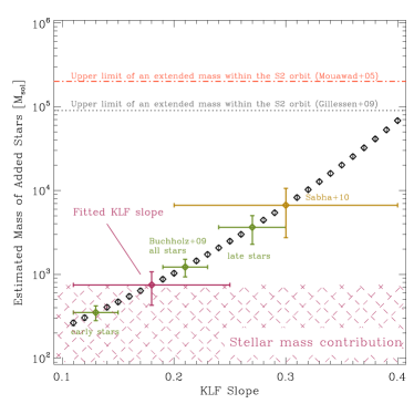
Figure 8: Estimated stellar mass from the added stars for different KLF slopes. Slopes of Buchholz et al. (2009) (for different stellar populations) are shown in green, NS10 in yellow and our fitted slope in purple. A limit imposed by the enclosed mass within the S2 orbit is plotted as horizontal dotted (gray) and dash-dotted (red) lines from Gillessen et al. (2009b) and Mouawad et al. (2005), respectively.

4 Dynamical probes of the distributed mass

If the gravitational force near Sgr A* includes contributions from bodies other than the SMBH, the orbits of test stars, including S2, will deviate from Keplerian ellipses. These deviations can be used to constrain the amount of distributed mass near Sgr A* (Mouawad et al. 2005; Gillessen et al. 2009b). But they can also be used to constrain the “granularity” of the perturbing potential, since the nature and magnitude of the orbital deviations depend both on the total mass of the perturbing stars, and on their individual masses.

Investigations of a single scattering event were explored by Gualandris et al. (2010) using high-accuracy N-body simulations and orbital fitting techniques. They found that an IMBH more massive than $10^{3}$ $M_{\odot}$, with a distance comparable to that of the S-stars, will cause perturbations of the orbit of S2 that can be observed after the next peribothron passage of S2. Here we examine the effect many scatterers (i.e. smaller masses for the scatterers but shorter impact parameters) will have on the trajectory of the star S2 as it orbits. Around Sgr A*, the stars and scatterers are moving in a potential well that is dominated by the mass of the central SMBH. In this case the encounters are of a correlated nature and hence cannot be considered as random events.

An important deviation from Keplerian motion occurs as a result of relativistic corrections to the equations of motion, which to lowest order predict an advance of the argument of peribothron, $\omega$, each orbital period of

$$\left(\Delta\omega\right)_{\mathrm{GR}}=\frac{6\pi GM_{\bullet}}{c^{2}a(1-e^{2})}.$$ (7)

Setting $a=5.0$ mpc and $e=0.88$ for the semi-major axis and eccentricity of S2, respectively, and assuming $M_{\bullet}=4.0\times 10^{6}$ $M_{\odot}$,

$$(\Delta\omega)_{\mathrm{GR}}\approx 10.8^{\prime}.$$ (8)

The relativistic precession is prograde, and leaves the orientation of the orbital plane unchanged.

The argument of peribothron also experiences an advance each period due to the spherically-symmetric component of the distributed mass. The amplitude of this “mass precession” is

$$\left(\Delta\omega\right)_{\mathrm{M}}=-2\pi G_{\mathrm{M}}(e,\gamma)\sqrt{1-e^{2}}\left[\frac{M_{\star}(r<a)}{M_{\bullet}}\right].$$ (9)

Here, $M_{\star}$ is the distributed mass within a radius $r=a$, and $G_{\mathrm{M}}$ is a dimensionless factor of order unity that depends on $e$ and on the power-law index of the density, $\rho\propto r^{-\gamma}$ (Merritt 2012). In the special case $\gamma=2$,

$$G_{\mathrm{M}}=\left(1+\sqrt{1-e^{2}}\right)^{-1}\approx 0.68\ \mathrm{for\ S2}$$ (10)

so that

$$\left(\Delta\omega\right)_{\mathrm{M}}\approx-1.0^{\prime}\;\left[\frac{M_{\star}(r<a)}{10^{3}\mathrm{\leavevmode\nobreak\ M}_{\odot}}\right].$$ (11)

Mass precession is retrograde, i.e., opposite in sense to the relativistic precession.

Since the contribution of relativity to the peribothron advance is determined uniquely by $a$ and $e$, which are known, a measured $\Delta\omega$ can be used to constrain the mass enclosed within S2’s orbit, by subtracting $(\Delta\omega)_{\mathrm{GR}}$ and comparing the result with Equation (11). So far, this technique has yielded only upper limits on $M_{\star}$ of $\sim 10^{-2}M_{\bullet}$ (Gillessen et al. 2009b).

The granularity of the distributed mass makes itself felt via the phenomenon of “resonant relaxation” (RR) (Rauch & Tremaine 1996; Hopman & Alexander 2006a). On the time scales of interest here, orbits near Sgr A* remain nearly fixed in their orientations, and the perturbing effect of each field star on the motion of a test star (e.g. S2) can be approximated as a torque that is fixed in time, and proportional to $m$, the mass of the field star. The net effect of the torques from $N$ field stars is to change the angular momentum, $\mathbf{L}$, of S2’s orbit according to

$$\frac{|\Delta\mathbf{L}|}{L_{c}}\approx K\sqrt{N}\frac{m}{M_{\bullet}}\frac{\Delta t}{P}$$ (12)

where $L_{c}=\sqrt{GM_{\bullet}a}$ is the angular momentum of a circular orbit having the same semi-major axis as that of the test star. (Equation 12 describes “coherent resonant relaxation”; on time scales much longer than orbital periods, “incoherent” resonant relaxation causes changes that increase as $\sim\sqrt{\Delta t}$.) The normalizing factor $K$ is difficult to compute from first principles but should be of order unity (Eilon et al. 2009). Changes in $\mathbf{L}$ imply changes in both the eccentricity, $e$, of S2’s orbit, as well as changes in its orbital plane. The latter can be described in a coordinate-independent way via the angle $\Delta\theta$, where

$$\cos(\Delta\theta)=\frac{\mathbf{L}_{1}\cdot\mathbf{L}_{2}}{L_{1}L_{2}}$$ (13)

and $\{\mathbf{L}_{1},\mathbf{L}_{2}\}$ are the values of $\mathbf{L}$ at two times separated by $\Delta t$. If we set $\Delta t$ equal to the orbital period of the test star, the changes in its orbital elements due to RR are expected to be

$$|\Delta e|_{\mathrm{RR}} \approx K_{e}\sqrt{N}\frac{m}{M_{\bullet}},$$ (14)

$$(\Delta\theta)_{\mathrm{RR}} \approx 2\pi K_{t}\sqrt{N}\frac{m}{M_{\bullet}},$$ (15)

where $N$ is the number of stars having $a$-values similar to, or less than, that of the test star and $\{K_{e},K_{t}\}$ are constants which may depend on the properties of the field-star orbits.

Because the changes in S2’s orbit due to RR scale differently with $m$ and $N$ than the changes due to the smoothly-distributed mass, both the number and mass of the perturbing objects within S2’s orbit can in principle be independently constrained. For instance, one could determine $M_{\star}=mN$ from Equations (7) and (11) and a measured $\Delta\omega$, then compute $m\sqrt{N}$ by measuring changes in $e$ or $\theta$ and comparing with Equations (14) or (15).

We tested the feasibility of this idea using numerical integrations. The models and methods were similar to those described in Merritt et al. (2010). The $N$ field stars were selected from a density profile $n(r)\propto r^{-2}$, with semi-major axes extending to $a_{\mathrm{max}}=8$ mpc. Initial conditions assumed isotropy in the velocity distribution. Two values for the field star masses were considered: $m=10$ $M_{\odot}$ and $m=50$ $M_{\odot}$. One of the $N$-body particles was assigned the observed mass and orbital elements of S2; this particle was begun at apobothron, and the integrations extended for one complete period of S2’s orbit. Each of the $N$ field-star orbits were integrated as well, and the integrator included the mutual forces between stars, as well as post-Newtonian corrections to the equations of motion. The quantities $\Delta\omega$, $\Delta e$ etc. for the S2 particle were computed by applying standard formulae to $(\mathbf{r},\mathbf{v})$ at the start and end of each integration. 100 random realizations of each initial model were integrated, allowing both the mean values of the changes, and their variance, to be computed.

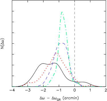
Figure 9: Histograms of the predicted change in S2’s argument of peribothron, $\omega$, over the course one orbital period ($\sim 16$ yr). The shift due to relativity, $(\Delta\omega)_{\mathrm{GR}}\approx 11^{\prime}$, has been subtracted from the total; what remains is due to Newtonian perturbations from the field stars. Each histogram was constructed from integrations of 100 random realizations of the same initial model, with field-star mass $m=10$ $M_{\odot}$, and four different values of the total number: $N=200$ (solid/black); $N=100$ (dotted/red); $N=50$ (dashed/blue); and $N=25$ (dot-dashed/green). The average value of the peribothron shift increases with increasing $Nm$, as predicted by Equation (11). The reasons for the spread in $\Delta\omega$ values are discussed in the text.

Figure 10: Average values of the changes in $\omega$, $e$ and $\theta$ for S2 over one orbital period ($\sim 16$ yr) in the $N$-body integrations. Filled circles are from integrations with $m=50$ $M_{\odot}$ and open circles are for $m=10$ $M_{\odot}$ ; the number of field stars was $N=\{25,50,100,200\}$ for both values of $m$. The abscissa is the distributed mass within S2’s apobothron, at $r\approx 9.4$ mpc. In each frame, the points are median values from the 100 $N$-body integrations, and the error bars extend from the $20$th to the $80$th percentile of the distribution. a) Changes in the argument of peribothron. The contribution from relativity, Equation (7), has been subtracted. The solid line is Equation (11). b) Changes in the eccentricity. Solid and dashed lines are Equation (14), with $m=50$ $M_{\odot}$ and $m=10$ $M_{\odot}$ respectively and with $K_{e}=1.4$. c) The angle between initial and final values of $\mathbf{L}$ for S2. Solid and dashed lines are Equations (15) with $K_{t}=1.0$.

Figures 9 and 10a show changes in $\omega$ for S2. The median change is well predicted by Equation (11). However there is a substantial variance. We identify at least two sources for this variance. (1) The number of stars inside S2’s orbit differs from model to model by $\sim\sqrt{N}$, resulting in corresponding changes to the enclosed mass, and hence to the precession rate as given by Equation (11). (2) When $N$ is finite, the same torques that drive resonant relaxation also imply a change in the field star’s rate of peribothron advance as compared with Equation (11), which assumes no tangential forces. While the dispersion scales roughly as $\sqrt{N}$, as evident in Figure 9, the fractional change in $\Delta\omega$ due to this effect scales as $\sim 1/\sqrt{N}$ (Merritt et al. 2010). Additional variance might arise from close encounters between field stars and S2, and from the fact that the mass within S2’s orbit is changing over the course of the integration due to the orbital motion of each field star.

Whereas the (average) value of $\Delta\omega$ depends only on the mass within S2’s orbit, the changes in $e$ and $\theta$ depend also on $m$, as shown in Figures 10b and c. The lines in those figures are Equations (14) and (15), with

$$K_{e}=1.4,\ \ \ \ K_{t}=1.0.$$

(We have defined $N$ in Equations (14) and (15) as the number of field stars inside a radius of $9.4$ mpc, the apobothron of S2.) For a given value of the enclosed mass, $M_{\star}=Nm$, Figure 10 shows that the changes in $e$ and $\theta$ indeed scale as $\sim 1/\sqrt{N}$ or as $\sim\sqrt{m}$, as predicted by Equations (14) and (15).

We can use these results to estimate the changes in $\omega$, $e$ and $\theta$ expected for S2, based on theoretical models of the distribution of stars and stellar remnants at the GC. In dynamically evolved models (Freitag et al. 2006; Hopman & Alexander 2006b), the total distributed mass within S2’s apobothron, $r\approx 10$ mpc, is predicted to be $\sim$ a few times $10^{3}$ $M_{\odot}$. About half of this mass is in the form of main-sequence stars and half in stellar-mass black holes, with a total number $N\approx 10^{3}$. When there are two mass groups, expressions like Equations (14) and (15) generalize to

$$|\Delta e|_{\mathrm{RR}} = K_{e}\left[\frac{m_{1}\sqrt{N_{1}}+m_{2}\sqrt{N_{2}}}{M_{\bullet}}\right]$$ (16)

$$(\Delta\theta)_{\mathrm{RR}} = 2\pi K_{t}\left[\frac{m_{1}\sqrt{N_{1}}+m_{2}\sqrt{N_{2}}}{M_{\bullet}}\right]$$ (17)

assuming

$$m_{1}=1\mathrm{\leavevmode\nobreak\ M}_{\odot},\quad m_{2}=10\mathrm{\leavevmode\nobreak\ M}_{\odot},\quad N_{1}=10^{3},\quad N_{2}=150$$

(Hopman & Alexander 2006b) we find

$$|\Delta e|_{\mathrm{RR}} \approx 5.4\times 10^{-5},$$ (18)

$$(\Delta\theta)_{\mathrm{RR}} \approx 0^{\prime}.8,$$ (19)

$$(\Delta\omega)_{\mathrm{M}} \approx -2.5^{\prime}.$$ (20)

For obtaining the dispersion in the value of Equation (20), we scaled the dispersion given in Figure 10a for the single population case, $N=50,m=50$ $M_{\odot}$ of the same total extended mass, to the two populations case we are investigating here. The dispersion obtained from the simulations is $\sim 4^{\prime}$. We scale it using the relation $\Delta\omega/\sqrt{N}$ in order to account for the SBH and MS populations, independently. The dispersion for the new configuration then becomes $\sim 1.43^{\prime}$, lower than the single population case. This is attributed to the fact that the number of main-sequence stars is much larger than the stellar-mass black holes, hence they lower the dispersion in the total Newtonian peribothron shift $(\Delta\omega)_{\mathrm{M}}$.

Considering a higher value for the enclosed mass $M_{\star}=10^{4}$ $M_{\odot}$ while keeping the same mass scales and abundance ratios of the scattering objects,

$$m_{1}=1\mathrm{\leavevmode\nobreak\ M}_{\odot},\quad m_{2}=10\mathrm{\leavevmode\nobreak\ M}_{\odot},\quad N_{1}=4000,N_{2}=600$$

one gets changes of

$$|\Delta e|_{\mathrm{RR}} \approx 1.1\times 10^{-4},$$ (21)

$$(\Delta\theta)_{\mathrm{RR}} \approx 1.7^{\prime},$$ (22)

$$(\Delta\omega)_{\mathrm{M}} \approx -10^{\prime}.$$ (23)

The dispersion in Equation (23) can be compared, as we did before, to the case considered in the simulations ($N=200,m=50$ $M_{\odot}$) by scaling the $\sim 8^{\prime}$ dispersion (Figure 10a) to become $\sim 2.86^{\prime}$ for the two mass population.

Repeating the same analysis as before to the $M_{\star}=10^{5}$ $M_{\odot}$ gives the following numbers for the stellar black holes and low-mass stars

$$m_{1}=1\mathrm{\leavevmode\nobreak\ M}_{\odot},\quad m_{2}=10\mathrm{\leavevmode\nobreak\ M}_{\odot},N_{1}=40000,N_{2}=6000$$

that result in

$$|\Delta e|_{\mathrm{RR}} \approx 3.4\times 10^{-4},$$ (24)

$$(\Delta\theta)_{\mathrm{RR}} \approx 5.2^{\prime},$$ (25)

$$(\Delta\omega)_{\mathrm{M}} \approx -100^{\prime}.$$ (26)

Similar to the above cases, the dispersion in Equation (26) can be compared to the single mass case by scaling the $\sim 25.3^{\prime}$ dispersion to become $\sim 9.1^{\prime}$ for the two mass population. The $\sim 25.3^{\prime}$ value is obtained by scaling with $\Delta\omega/\sqrt{N}$ from the value shown in Figure 10a for the $10^{4}$ $M_{\odot}$ extended mass.

We would like to stress that making a definite prediction about the $N$-dependence of the variance is beyond the scope of the current paper. However, we have noted that in both cases considered in Figure 10 the relative variance is of the order of unity or larger i.e. the dispersion is of the order of the Newtonian peribothron shift.

The positional uncertainty is currently of the order of 1 mas. For the highly eccentric orbit of S2 this implies that the accuracy with which the peribothron shift can be detected is of the order of $24^{\prime}$. As can be seen for the case of $M_{\star}=10^{5}$ $M_{\odot}$ , the shifts are at the limit of the current instrumental capabilities if the total enclosed mass was entirely composed of massive perturbers. The shifts given in Equations (20) and (23) can be measured if the accuracy is improved by at least one order of magnitude using larger telescopes or interferometric methods in the NIR. However, considering the variances in the calculated shifts one would need to observe more than one stellar orbit in order to infer information on the population giving rise to the Newtonian peribothron shift. By comparison, the current uncertainty in S2’s eccentricity is $\sim 0.003$, and uncertainties in the Delaunay angles $i$ and $\Omega$ describing its orbital plane are $\sim 50^{\prime}$ (Gillessen et al. 2009b). In both cases, an improvement of a factor $\sim 50$ would be required in order to detect the changes given in $e$ and $\theta$.

Dynamically-relaxed models of the GC have been criticized on the grounds that they predict a steeply-rising density of old stars inside $\sim 1$ pc, while the observations show a parsec-scale core (Buchholz et al. 2009; Do et al. 2009; Bartko et al. 2010). Dynamically unrelaxed models imply a much lower density near Sgr A* and an uncertain fraction of stellar-mass black holes (Merritt 2010; Antonini et al. 2012). The number of perturbers is so small in these models that their effect on the orbital elements of S2 would be undetectable for the foreseeable future, barring a lucky close encounter with S2.

In addition to the small amplitude of the perturbations, the potential difficulty in constraining $N$ and $m$ comes from the nonzero variance of the predicted changes (Figure 10). The variance in $\Delta\omega$ scales as $\sim\Delta\omega/\sqrt{N}$ and would be small in the dynamically-relaxed models with $N\approx 10^{3}$. Another source of uncertainty comes from the dependence of the amplitude of $\Delta\omega$ on $\gamma$ (Equation 9), which is unknown. We do not have a good model for predicting the variances in $|\Delta e|$ and $\Delta\theta$, but Figure 10 suggests that the fractional variance in these quantities is not a strong function of $N$ or $m$, and that it is large enough to essentially obscure changes due to a factor $\sim 5$ change in $m$ at fixed $M_{\star}$. On the other hand, considerably more information might be available than just $\Delta e$ and $\Delta\theta$ for one star; for instance, the full time-dependence of $(\mathbf{r},\mathbf{v}$) for a number of stars. We leave a detailed investigation of how well such information could constrain the perturber $m$ and $N$ to a future work.

4.1 Fighting the limits on the power of stellar orbits

The results from the previous sub-sections clearly show that deriving the net-displacement for an ideal elliptical orbit for a single star will not be sufficient to put firm limits on both the total amount of extended mass and on the nature of the corresponding population. However, the situation may be improved if one studies the statistics of the time and position dependent deviations along a single star’s orbit or instead uses the orbits of several stars.

4.1.1 Improving the single orbit case

The actual uncertainty in projected right ascension or declination, $\sigma_{\mathrm{position}}^{2}$, can be thought of as a combination of several contributions. Here $\sigma_{\mathrm{apparent}}^{2}$ is the apparent positional variation due to the photo-center variations of the star while it is moving across the sea of fore- and background sources. The scattering process results in a variation of positions described by $\sigma_{\mathrm{scattering}}^{2}$. Finally, systematic uncertainties due to establishing and applying an astrometric reference frame give a contribution of $\sigma_{\mathrm{systematic}}^{2}$.

The value of $\sigma_{\mathrm{position}}^{2}$ can be measured in comparison to the orbital fit. The value of $\sigma_{\mathrm{apparent}}^{2}$ can be obtained experimentally by placing an artificial star into the imaging frames at positions along the idealized orbit. A reliable estimate of $\sigma_{\mathrm{apparent}}^{2}$ is achieved by comparing the known positions at which the star has been placed and the positions measured in the image frames. As for the case of the systematic variations, they can be estimated by investigating sources that are significantly brighter or slower than the S-stars. Finally, the value that describes the scattering process, and therefore gives information on the masses of the scattering sources, can be obtained via

$$\sigma_{\mathrm{scattering}}^{2}=\sigma_{\mathrm{position}}^{2}-\sigma_{\mathrm{apparent}}^{2}-\sigma_{\mathrm{systematic}}^{2}.$$ (27)

Alternatively, $\sigma_{\mathrm{scattering}}^{2}$ could be measured directly by near-infrared interferometry with long baselines. Measuring the position of S2 interferometrically as a function of time with respect to bright reference objects could allow observing the effects of single scattering events. Here the assumption is that they happen infrequently enough such that one can build up sufficient signal to noise on the $\sigma_{\mathrm{scattering}}$ measurement provided that the uncertainties in the interferometric measuring process are sufficiently well known.

4.1.2 Improving by using several stars

If scattering events contribute significantly to the uncertainties in the determination of the orbits, a number of stars may help to derive the physical properties of the medium through which the stars are moving. While the influence of the extended mass imposes a systematic variation of the orbits through the Newtonian peribothron shift, the variations due to scattering events will be random. This implies that for individual stars the effects may partially compensate or amplify each other. Averaging the results of $N$ stars, that will then essentially sample the shape of the distributions shown in Figure 9, may therefore result in an improvement proportional to $N^{-1/2}$ in the determination of the extended mass.

5 Simulating the distribution of fainter stars

In NS10 we detected three stars that were either previously not identified at all (NS1 & NS2 stars, Figure 1 in NS10) or only allowed an unsatisfactory identification with previously known members of the cluster (S62, as pointed out in Dodds-Eden et al. 2011). In addition we have the case of the star S3 which was identified in the $K_{\mathrm{s}}$-band in the early epochs 1992 (Eckart & Genzel 1996), 1995 (Ghez et al. 1998) and lost after about 3 years in 1996/7 (Ghez et al. 1998), 1998 (Genzel et al. 2000). We investigate this phenomenon in our modeling by extrapolating the KLF in the inner 1–2 arcsec region, surrounding Sgr A*, to stars fainter than the faintest source ($K_{\mathrm{s}}=17.31$) we detected in our 30 August and 23 September 2004 dataset, in which Sgr A* shows very low activity (NS10). In this section we describe the method we use to simulate the distribution of these faint stars, and the possible false detections that can be caused by the combined light of many stars appearing in projection to be very close to each other, such that they cannot be individually resolved with 8–10 m class telescopes.

The calculations were done by taking all the extra (extrapolated) faint stars in the $K_{\mathrm{s}}$-magnitude interval of 18 to 25. The stars were then distributed in a $23\times 23$ grid that corresponds to 529 cells. Each cell has the dimensions of $0.06^{\prime\prime}\times 0.06^{\prime\prime}$, i.e. about one angular resolution element in $K_{\mathrm{s}}$-band, this grid, therefore, simulates observations of the inner $1.38^{\prime\prime}\times 1.38^{\prime\prime}$ projected region surrounding Sgr A*. We distributed the faint stars in the grid such that their radial profile centered on Sgr A* reproduces that of the stellar number density counts of the inner region of the central stellar cluster with a power-law index of $\Gamma=0.30\pm 0.05$ from Schödel et al. (2007). This way each cell has a specific number of stars that can be inserted into it, with the maximum number of stars being located in the central cell, i.e. the peak of the radial profile. Our algorithm fills each cell with its specified number of stars by choosing them randomly from a pool of stars created from the extrapolated KLF. The pool is created such that for each $K_{\mathrm{s}}$-magnitude bin above $\sim 18$, a number of stars $N$ get their $K_{\mathrm{s}}$-band magnitudes according to the KLF. From this pool of stars we then randomly pick objects to fill the cells of the grid such that they obey the power-law radial number density profile. Then, the fluxes of the stars in each individual cell are added up and compared to the value of 0.76 mJy which is the flux density of the faintest stellar source in our S-star cluster data, i.e. $K_{\mathrm{s}}=17.31$ (NS10). We ran the simulation $10^{4}$ times in order to get reliable statistical estimates for the brightnesses in each resolution cell. Hence we can estimate how likely it is to find strong apparent clusterings along the line of sight that are brighter than the faintest star we identified in the S-cluster (flux larger than 0.76 mJy).

Table 1: Probabilities of detecting a false star (brighter than $K_{\mathrm{s}}=17.31$) in a $1.38^{\prime\prime}\times 1.38^{\prime\prime}$ region.

$K_{\mathrm{s}}$-band	Power-law index
magnitude
cutoff	0.19	0.30	0.35
KLF slope $=0.11$
20.99	$0.0000$	$0.1471$	$0.1500$
24.67	$0.0285$	$0.0292$	$0.0224$
KLF slope $=0.18$
20.99	$0.0848$	$0.1286$	$0.3016$
24.67	$0.2058$	$0.2426$	$0.2927$
KLF slope $=0.25$
20.99	$0.7776$	$0.7442$	$0.9085$
24.67	$0.9462$	$0.9725$	$0.9802$

Taking into account the uncertainties of the quantities that describe the central S-star cluster we have repeated the simulation for a combination of three KLF slopes ($0.11$, $0.18$ and $0.25$), three radial profile power-law indices ($\Gamma=0.19$, $0.30$ and $0.35$) and two $K_{\mathrm{s}}$-magnitude cutoffs for the extrapolation, $21$ and $25$ (corresponding to 0.0258 and 0.0009 mJy, respectively). Here the brighter cutoff is very close to the brightness of the faintest stars that have been detected. The choice for the KLF slope satisfies the range of the power-law fit $\Gamma=0.18\pm 0.07$. The power-law indices were taken from Table 5 of Schödel et al. (2007) for the cusp radial profiles.

The results of the simulations are summarized in Table 1. Three different realizations of a cluster simulation as well as the average of $10^{4}$ simulations are shown in Figure 11. We find that for the measured KLF slope of $0.18$, a measured power-law index of $\Gamma=0.3$ and a faint $K_{\mathrm{s}}$-magnitude cutoff we obtain a false star in about a quarter of all simulations. For steeper KLF and power-law slopes $\Gamma$ we get this result in more than 70% of all cases independent of the cutoff magnitude.

Table 2: Probabilities of detecting a false star (brighter than $K_{\mathrm{s}}=17.31$) at the position of Sgr A*.

$K_{\mathrm{s}}$-band	Power-law index
magnitude
cutoff	0.19	0.30	0.35
KLF slope $=0.11$
20.99	$0.0000(2)$	$0.0752(4)$	$0.0757(4)$
24.67	$0.0094(6)$	$0.0103(6)$	$0.0099(6)$
KLF slope $=0.18$
20.99	$0.0423(4)$	$0.0438(4)$	$0.1181(5)$
24.67	$0.0345(15)$	$0.0591(18)$	$0.0821(20)$
KLF slope $=0.25$
20.99	$0.3120(8)$	$0.3149(8)$	$0.5448(10)$
24.67	$0.3223(59)$	$0.4756(70)$	$0.5291(74)$

In Table 2 we show the same statistics as in Table 1 but for the central cell in the grid, at the projected position of Sgr A*. Also given, in parentheses, is the number of stars in the central cell that gives rise to the detection of a false star at a distance of less than one angular resolution element away from the line of sight to Sgr A*. We find that for a KLF slope of $0.25$ we get a false star in 30% to 50% of all simulations, independent of the power-law index $\Gamma$ and the cutoff magnitude. This is consistent with the offsets found in different observational epochs of Sgr A* light curves (Witzel et al. 2012; Dodds-Eden et al. 2011). In this case the blend consists of 8 to 74 stars below the unresolved background in the S-star cluster region. For flatter KLF slopes (i.e. 0.11 and 0.18) we find that a blend star only occurs in less than about 10% of all cases, which appears to be well below the upper limit found from observations. For a KLF slope of $\alpha=0.25$ and a number density power-law index of $\Gamma$ around 0.3 the total number of stars in the simulated S-star cluster is a few 1000. This is consistent with the number of main-sequence stars assumed by Freitag et al. (2006).

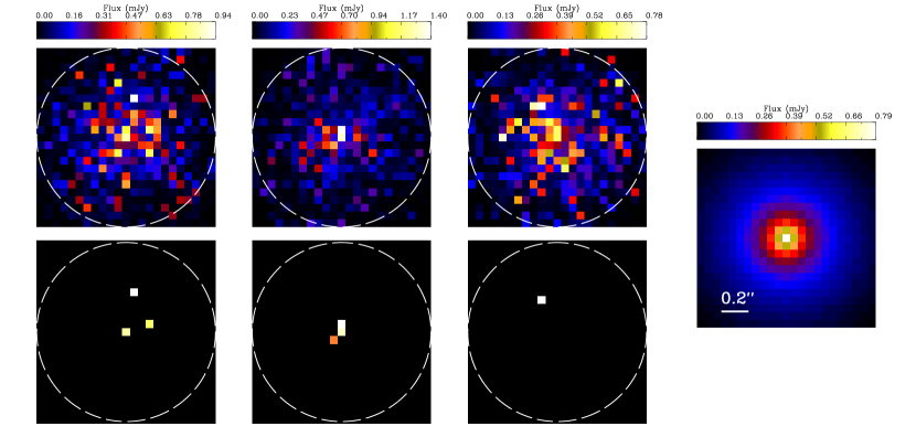
Figure 11: Upper panel: Three different snapshots of the simulation for the 0.25 KLF slope, power-law index $\Gamma=0.3$ and 24.67 $K_{\mathrm{s}}$-magnitude cutoff. Lower panel: The same as upper but with only the detectable blend stars visible. Right: Average of all the $10^{4}$ simulation snapshots for the same setup.

6 Summary and conclusion

By determining the KLF of the S-star cluster members from infrared imaging, using the distribution of the diffuse background light and the stellar number density counts, we have been able to shed some light on the amount and nature of the stellar and dark mass associated with the cluster of high velocity S-stars in the immediate vicinity of Sgr A*.

The amount of light from the fainter S-cluster members is below the amount of residual light after removing the bright cluster members. One implication could be that both the diffuse light and dark mass are overestimated. However, while NS10 estimate that only a maximum of one third of the diffuse light could be due to residuals from the PSF subtraction, we find that faint stars at or beyond the completeness limit reached in the KLF can account only for about 15% of the background light. Additional light may also originate from accretion processes onto a large number of 10 $M_{\odot}$ black holes that may reside in the central region, covered by the S-stars. We find that the stellar mass derived from the KLF extrapolation is much smaller than the amount of mass that may be present considering the uncertainties in the orbital motion of the star S2. Higher angular resolution and sensitivity are needed to resolve the background light and analyze its origin.

By investigating the effects of orbital torques due to resonant relaxation, we find that if a significant population of 10 $M_{\odot}$ black holes is present, with enclosed masses between $10^{3}$ $M_{\odot}$ and $10^{5}$ $M_{\odot}$ (see e.g. Freitag et al. 2006), then for trajectories of S2-like stars, contributions from scattering will be important compared to the relativistic or Newtonian peribothron shifts. This clearly shows that observing a single stellar orbit will not be sufficient to put firm limits on the total amount of extended mass and on the importance of relativistic peribothron shift. In this case only the observation of a larger number of stars will allow to sample the statistics of the effect, i.e. the distributions in Figure 9. However, if the distribution of 10 $M_{\odot}$ black holes is cuspy then this may become even more difficult (and close encounters should be frequent in this region).

In general, the inclusion of star-star perturbations allows us to probe the distribution and composition of mass very close to the SMBH simultaneously, if the astrometric accuracy can be improved by an order of magnitude by using either larger telescopes or interferometers in the NIR.

With measurements and extrapolations of the S-star cluster KLF slope, and number density counts with assumptions on the KLF cutoff magnitude, we can show that the contamination for the members of the cluster, and especially at the position of Sgr A*, by blend stars is fully consistent with measurements. We show that for 8–10 m class telescopes the presence and proper motion of faint stars close to the confusion limit in the region of the S-star cluster is highly contaminated by blend stars. Due to the 2-dimensional velocity dispersion of the stars within the S-star cluster of about 600 km/s the blend stars will last for about 3–4 years before they fade and dissolve. Close to the center, we find the probability of detecting blend stars at any time is about 30–50%. At the central position the change from the appearance of a blend star to the appearance of another may also give the illusion of high proper motions for 8–10 m class telescopes. Such a prime example would be S3, detected close to the position of Sgr A*, which had both a limited lifetime and high proper motion (Eckart & Genzel 1996; Ghez et al. 1998; Genzel et al. 2000). Blending of sources along the line of sight may also severely contaminate the proper motion measurements of individual stars close to the confusion limit. Only with the help of proper motion measurements over time significantly longer than 3 years one will be able to derive reliable orbital parameters for a single star. Also, spectroscopy may help to resolve blend stars, however, the objects are faint and spectroscopy will be difficult.

These findings clearly demonstrate the necessity of higher angular resolution, astrometric accuracy and point source sensitivity for future investigations of the S-star cluster. They would also greatly improve the derivation of the amount and the compactness of the central mass as well as the determination of relativistic effects in the vicinity of Sagittarius A*.