Rapidly Accreting Supergiant Protostars:
Embryos of Supermassive Black Holes?

Abstract

Direct collapse of supermassive stars (SMSs) is a possible pathway for generating supermassive black holes in the early universe. It is expected that an SMS could form via very rapid mass accretion with $\dot{M}_{*}\sim 0.1-1~{}M_{\odot}~{}{\rm yr}^{-1}$ during the gravitational collapse of an atomic-cooling primordial gas cloud. In this paper we study how stars would evolve under such extreme rapid mass accretion, focusing on the early evolution until the stellar mass reaches $10^{3}~{}M_{\odot}$. To this end we numerically calculate the detailed interior structure of accreting stars with primordial element abundances. Our results show that for accretion rates higher than $10^{-2}~{}M_{\odot}~{}{\rm yr}^{-1}$, stellar evolution is qualitatively different from that expected at lower rates. While accreting at these high rates the star always has a radius exceeding $100~{}R_{\odot}$, which increases monotonically with the stellar mass. The mass-radius relation for stellar masses exceeding $\sim 100~{}M_{\odot}$ follows the same track with $R_{*}\propto M_{*}^{1/2}$ in all cases with accretion rates $\gtrsim 10^{-2}~{}M_{\odot}~{}{\rm yr}^{-1}$; at a stellar mass of $10^{3}~{}M_{\odot}$ the radius is $\simeq 7000~{}R_{\odot}$ ($\simeq 30$ AU). With higher accretion rates the onset of hydrogen burning is shifted towards higher stellar masses. In particular, for accretion rates exceeding $\dot{M}_{*}\gtrsim 0.1~{}M_{\odot}~{}{\rm yr}^{-1}$, there is no significant hydrogen burning even after $10^{3}~{}M_{\odot}$ have accreted onto the protostar. Such “supergiant” protostars have effective temperatures as low as $T_{\rm eff}\simeq 5000$ K throughout their evolution and because they hardly emit ionizing photons, they do not create an HII region or significantly heat their immediate surroundings. Thus, radiative feedback is unable to hinder the growth of rapidly accreting stars to masses in excess of $10^{3}~{}M_{\odot}$, as long as material is accreted at rates $\dot{M}_{*}\gtrsim 10^{-2}~{}M_{\odot}~{}{\rm yr}^{-1}$.

1. Introduction

Recent observations reveal that supermassive black holes (SMBHs) exceeding $10^{9}~{}M_{\odot}$ already existed in the universe less than 1 Gyr after the Big Bang (e.g., Fan, 2006; Mortlock et al., 2011; Treister et al., 2011). The origins of such SMBHs must be intimately related to structure formation in the early universe. Some scenarios on the birth and growth of SMBHs postulate the existence of remnant BHs from Population III (Pop III) stars as their seeds (e.g., Madau & Rees, 2001; Schneider et al., 2002). For several decades theoretical studies have predicted that the majority of Pop III stars were very massive, exceeding $100~{}M_{\odot}$ (e.g., Bromm & Larson, 2004). Pop III stars more massive than $300~{}M_{\odot}$ end their lives by directly collapsing to form BHs (e.g., Heger & Woosley, 2002). If such a $\sim 100~{}M_{\odot}$ BH grows via continuous mass accretion at the Eddington limited rate, its mass barely attains $10^{9}~{}M_{\odot}$ in 1 Gyr.

This scenario, however, has recently been challenged. First, it is suspected that most Pop III stars were much less massive than previously thought. A circumstellar disk forming after the cloud’s collapse easily fragments due to gravitational instability and could produce multiple protostars (e.g., Machida et al., 2008; Stacy et al., 2010; Clark et al., 2011). The final stellar masses would be reduced as the accreting gas is shared by multiple stars. Moreover, strong stellar UV light creates an HII region around the protostar when the stellar mass exceeds a few $\times 10~{}M_{\odot}$. The resulting feedback terminates the growth of Pop III protostars via mass accretion at a few $\times 10~{}M_{\odot}$ (e.g., McKee & Tan, 2008; Hosokawa et al., 2011b; Stacy et al., 2012). A large amount of gas would be expelled from the dark halo due to the expansion of HII regions and the onset of core-collapse supernovae (e.g., Whalen et al., 2004; Kitayama et al., 2004; Kitayama & Yoshida, 2005), which quenches the supply of gas to any remnant BH. Even if a BH gets some gas supply, radiative feedback from the BH accretion disk could regulate mass accretion onto the BH-disk system (e.g., Alvarez et al., 2009; Milosavljević et al., 2009; Jeon et al., 2011).

Another pathway for generating SMBHs is BH binary mergers. However, this process could be also limited due to the strong recoil resulting from gravitational wave emission (e.g., Campanelli et al., 2007; Herrmann et al., 2007). It is not straightforward that a seed BH $\lesssim 100~{}M_{\odot}$ can grow to a $\sim 10^{9}~{}M_{\odot}$ SMBH within 1 Gyr of its birth.

An alternative possibility is that massive BHs exceeding $10^{5}~{}M_{\odot}$ form directly in some rare occasions in the primordial gas (e.g., Bromm & Loeb, 2003). The primary cooling process in the primordial gas is line emission of molecular hydrogen. However, the thermal evolution of a gravitationally collapsing cloud can change significantly, if this cooling process is suppressed, for example, due to photodissociation of molecules by strong background radiation (Omukai, 2001; Oh & Haiman, 2002; Shang et al., 2010; Inayoshi & Omukai, 2011) or collisional dissociation in dense shocks (Inayoshi & Omukai, 2012). If the dark halo is sufficiently massive ($\gtrsim 10^{8}M_{\odot}$), the baryonic gas can contract with atomic hydrogen cooling even without molecular hydrogen. The collapse proceeds nearly isothermally at $\simeq 8000$ K. Without efficient molecular cooling fragmentation is suppressed and single or binary protostars form within dense cloud cores of $\gtrsim 10^{5}~{}M_{\odot}$ (Bromm & Loeb, 2003; Regan & Haehnelt, 2009). The protostar’s mass is initially $\sim 10^{-2}~{}M_{\odot}$ but quickly increases via mass accretion. The expected accretion rates are $0.1-1~{}M_{\odot}~{}{\rm yr}^{-1}$, more than 100 times higher than the standard value $\simeq 10^{-3}~{}M_{\odot}~{}{\rm yr}^{-1}$ expected for Pop III star formation. The stellar mass could reach $10^{5-6}~{}M_{\odot}$ in $\sim 1$ Myr with this very rapid mass accretion. General relativity predicts that such a supermassive star (SMS) becomes unstable (e.g. Chandrasekhar, 1964) and collapses to form a BH, which subsequently swallows most of the surrounding stellar material (e.g., Shibata & Shapiro, 2002). Some authors are exploring a different picture, whereby only a central part of the SMS collapses to form a $\sim 100~{}M_{\odot}$ BH and heat input from the accreting BH inflates the outer envelope of the SMS (”quasi-star”, Begelman et al., 2006, 2008; Begelman, 2010; Ball et al., 2011; Dotan et al., 2011).

However, we only have limited knowledge on how stars evolve under such extreme conditions of rapid mass accretion. Begelman (2010) predicts that, based on simple analytic arguments, such stars have a very different structure from their main-sequence counterparts. Stellar evolution at lower accretion rates $\dot{M}_{*}\lesssim 10^{-2}~{}M_{\odot}~{}{\rm yr}^{-1}$ has been studied in detail by numerically solving the stellar interior structure (e.g., Stahler et al., 1986; Omukai & Palla, 2001, 2003; Ohkubo et al., 2009; Hosokawa & Omukai, 2009; Hosokawa et al., 2010). Omukai & Palla (2001, 2003) showed that rapid mass accretion with $\dot{M}_{*}>4\times 10^{-3}~{}M_{\odot}~{}{\rm yr}^{-1}$ causes the protostar’s abrupt expansion before its arrival to the Zero-Age Main Sequence (ZAMS). Further comprehensive studies on stellar evolution with rapid mass accretion are indispensable for considering their radiative feedback and observational signatures (e.g., Johnson et al., 2011).

We present here our first results of this sort, whereby as a first step, we study the early evolution up to a stellar mass of $10^{3}~{}M_{\odot}$. Our results show that rapid accretion with $\dot{M}_{*}\gtrsim 10^{-2}~{}M_{\odot}~{}{\rm yr}^{-1}$ causes the star to bloats up like a red giant. The stellar radius increases monotonically with stellar mass and reaches $\simeq 7000~{}R_{\odot}(\simeq 30$ AU) at a mass of $10^{3}~{}M_{\odot}$. Unlike the cases with lower accretion rates previously studied, the mass-radius relation in this phase is almost independent of the assumed accretion rate. Such massive “super-giant” protostars could be the progenitors that eventually evolve to the observed SMBHs in the early universe.

The organization of this paper is as follows. First, we briefly review our numerical method and summarize the calculated cases in Section 2. We describe our results in Section 3; we first focus on the fiducial case with $\dot{M}=0.1~{}M_{\odot}~{}{\rm yr}^{-1}$ and then examine effects of varying accretion rates and boundary conditions. Finally, summary and discussions are described in Section 4.

Table 1 Cases Considered

Case	$\dot{M}_{*}$ ($M_{\odot}~{}{\rm yr}^{-1}$)	$M_{*,0}$ ($M_{\odot}$)	$R_{*,0}$ ($R_{\odot}$)	Notes	References
MD1e0	$1.0$	2.5	298.4		Sec. 3.2
MD3e1	$0.3$	2.0	238.3		Sec. 3.2, 3.3
MD3e1-HC10	$0.3$	2.0 (10)	238.3 (437.1)	shock $\to$ photo. BC at $M_{*}=10~{}M_{\odot}$	Sec. 3.3
MD3e1-HC50	$0.3$	2.0 (50)	238.3 (826.8)	shock $\to$ photo. BC at $M_{*}=50~{}M_{\odot}$	Sec. 3.3
MD1e1	$0.1$	2.0	177.8	fiducial case	Sec. 3.1, 3.2
MD6e2	$0.06$	1.0	118.6		Sec. 3.2
MD3e2	$0.03$	1.0	95.2		Sec. 3.2
MD6e3	$0.006$	1.0	52.3	also see Omukai & Palla (2003)	Sec. 3.2
MD1e3	$0.001$	0.05	12.5	also see Omukai & Palla (2003)	Sec. 3.1, 3.2

Note. — Col. 2: mass accretion rate, Col. 3: initial stellar mass, Col. 4: initial radius. For cases MD3e1-HC10 and MD3e1-HD50 the values when the boundary condition is switched is given in parentheses.

2. Numerical Modeling of Accreting Stars

2.1. Method

We calculate stellar evolution with mass accretion using the numerical codes developed in our previous work (see Omukai & Palla, 2003; Hosokawa & Omukai, 2009; Hosokawa et al., 2010, for details). The four stellar structure equations, i.e., equations of continuity, hydrostatic equilibrium, energy conservation, and energy transfer, including effects of mass accretion are solved assuming spherical symmetry. We focus on the early evolution until slightly after the ignition of hydrogen fusion in this paper. To this end, the appropriate nuclear network for the thermo-nuclear burning of deuterium, hydrogen, and helium is considered.

The codes are designed to handle two different outer boundary conditions for stellar models: shock and photospheric boundaries. The shock boundary condition presupposes spherically symmetric accretion onto a protostar, whereby the inflow directly hits the stellar surface and forms a shock front (e.g., Stahler et al., 1980; Hosokawa & Omukai, 2009). We solve for the structure of both the stellar interior and outer accretion flow. With this boundary condition the photosphere is located outside the stellar surface where the accretion flow is optically thick to the stellar radiation. The photospheric boundary condition, on the other hand, presupposes a limiting case of mass accretion via a circumstellar disk, whereby accretion columns connecting the star and disk are geometrically compact and most of the stellar surface radiates freely (e.g., Palla & Stahler, 1992; Hosokawa et al., 2010). In this case we only solve the stellar interior structure without considering details of the accretion flow; the location of photosphere always coincides with the stellar surface.

The different outer boundary conditions correspond to the two extremes of accretion flow geometries, or more specifically to different thermal efficiencies of mass accretion, which determine the specific entropy of accreting materials (e.g., Hosokawa et al., 2011a). The accretion thermal efficiency controls the entropy content of the star, which determines the stellar structure. With the shock boundary condition, the accreting gas obtains a fraction of the entropy generated behind the shock front at the stellar surface. The resulting thermal efficiency is relatively high (“hot” accretion).

For the photospheric boundary condition, on the other hand, the accreting gas is assumed to have the same entropy as in the stellar atmosphere. The underlying idea is that, when the accreting gas slowly approaches the star via angular momentum transport in the disk, its entropy should be regulated to the atmospheric value. This is a limiting case of thermally inefficient accretion (“cold” accretion). In general, with even a small amount of angular momentum, mass accretion onto the protostar would be via a circumstellar disk, perhaps with geometrically narrow accretion columns connecting the disk with the star. For extremely rapid mass accretion, however, the innermost part of the disk becomes hot and entropy generated within the disk is advected into the stellar interior (e.g., Popham et al., 1993). Thus, cold accretion as envisioned for the photospheric boundary condition is not appropriate for the case of rapid mass accretion (also see discussions in Hartmann et al., 1997; Smith et al., 2011). We therefore expect that the shock boundary condition is a good approximation for the extremely high accretion rates considered here and mostly focus on stellar evolution with the shock boundary condition. We also consider a few cases with the photospheric boundary condition for comparison to test potential effects of reducing the accretion thermal efficiency (also see Sec. 2.2 below).

2.2. Cases Considered

The cases considered are summarized in Table 1. In this paper, we only consider the evolution with constant accretion rates for simplicity. The adopted accretion rates range from $10^{-3}~{}M_{\odot}~{}{\rm yr}^{-1}$ to $1~{}M_{\odot}~{}{\rm yr}^{-1}$. Stellar evolution with accretion rates less than $10^{-2}~{}M_{\odot}~{}{\rm yr}^{-1}$ (cases MD1e3 and MD6e3) has been studied in detail in our previous work (e.g., Omukai & Palla, 2003; Hosokawa & Omukai, 2009). As described in Section 2.1 above, we calculate the protostellar evolution assuming shock outer boundary conditions for most of the cases. Cases MD3e1-HC10 and MD3e1-HC50 are the only exceptions, whereby we switch to the photospheric boundary condition after the stellar mass reaches $10~{}M_{\odot}$ and $50~{}M_{\odot}$, respectively, at a constant accretion rate $0.3~{}M_{\odot}~{}{\rm yr}^{-1}$. The underlying idea for switching the boundary at some moment is that the specific angular momentum of the inflow and thus the circumstellar disk grows with time, which reduces entropy of the accreted matter. The higher mass at switching point corresponds to the higher angular momentum of the parental core. As in our previous work, we start the calculations with initial stellar models constructed assuming that the stellar interior is in radiative equilibrium (e.g., Hosokawa & Omukai, 2009). We adopt a slightly higher initial stellar mass of $\sim 1M_{\odot}$ for stability reasons. The calculated initial stellar radii are also summarized in Table 1.

3. Results

3.1. Evolution in the Fiducial Case ($\dot{M}_{*}=0.1~{}M_{\odot}~{}{\rm yr}^{-1}$)

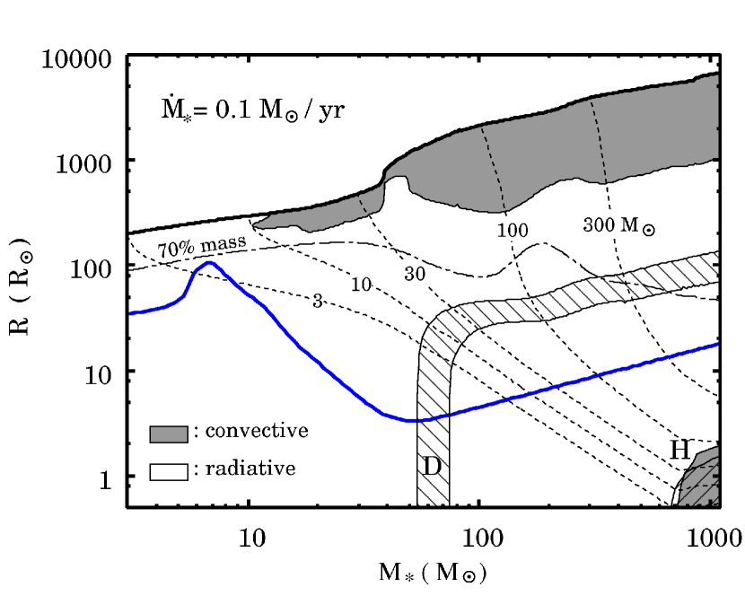
Figure 1.— Evolution of the stellar interior structure for the fiducial case, whereby the stellar mass increases at a rate of $0.1~{}M_{\odot}~{}{\rm yr}^{-1}$ (case MD1e1). The thick solid line depicts the stellar surface, which is the position of the accretion shock front. The dotted lines show the radial positions of the mass coordinates of $M=3$, 10, 30, 100, and $300~{}M_{\odot}$. The dot-solid line indicates the radial position within which 70 % of the stellar mass is enclosed. The gray-shaded areas represent the convective layers. The hatched areas indicate layers of active nuclear burning, where the energy production rate exceeds 10% of the steady rate $0.1L_{\rm D,st}/M_{\ast}$ for deuterium burning (see eq. 3.1), and $0.1L_{\ast}/M_{\ast}$ for hydrogen burning. The blue solid line shows the evolution of the radius of a star accreting material at $10^{-3}~{}M_{\odot}~{}{\rm yr}^{-1}$ for comparison.

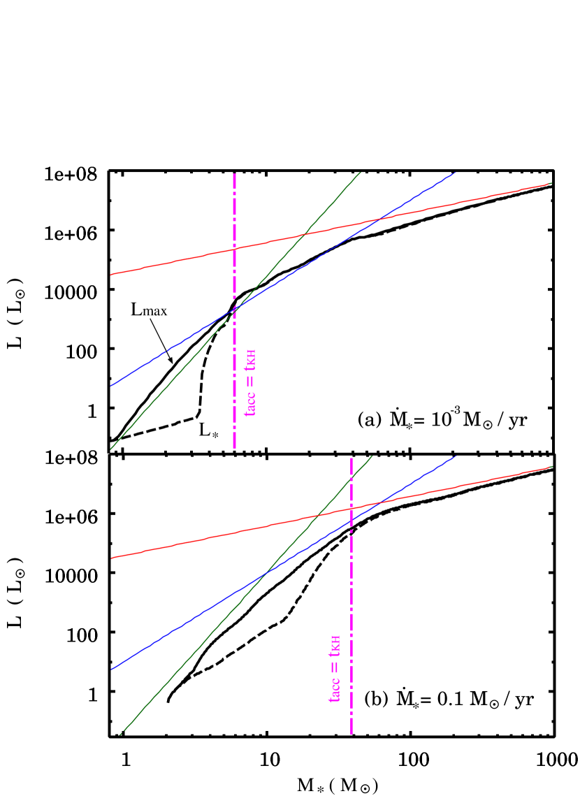
Figure 2.— Evolution of the stellar surface luminosity $L_{*}$ (dashed line) and maximum luminosity within the star $L_{\rm max}$ (solid line) for the cases with $10^{-3}~{}M_{\odot}~{}{\rm yr}^{-1}$ (MD1e3; upper panel) and $0.1~{}M_{\odot}~{}{\rm yr}^{-1}$ (fiducial case MD1e1; lower panel). The mass-luminosity relations given by equations (3), (4) and (5) are shown with the thin green, blue, and red lines, respectively. In each panel the vertical dot-dashed line (magenta) indicates the epoch when the accretion time is equal to the KH time.

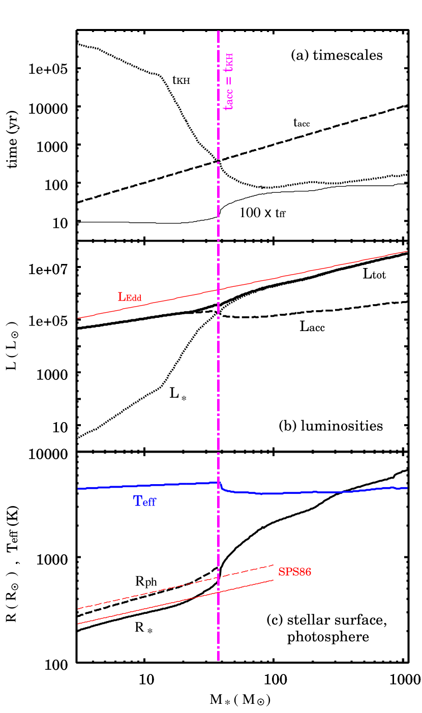
Figure 3.— Evolution of several physical quantities for the fiducial case with $0.1~{}M_{\odot}~{}{\rm yr}^{-1}$ (MD1e1). Top panel: Comparison between the accretion timescale $t_{\rm acc}$ (dashed line) and KH timescale $t_{\rm KH}$ (dotted line). The vertical magenta dot-dashed line indicates the epoch when $t_{\rm KH}$ is equal to $t_{\rm acc}$. The thin solid line represents 100 times of the stellar free-fall timescale $t_{ff}\equiv\sqrt{3\pi/32G\bar{\rho}}$, where $\bar{\rho}$ is the average mass density of the star. The fact that $t_{ff}$ is much shorter than $t_{\rm KH}$ and $t_{\rm acc}$ verifies the hydrostatic balance assumption implicit in the stellar structure equations. Middle panel: Evolution of the accretion luminosity $L_{\rm acc}$ (dashed line), stellar luminosity $L_{*}$ (dotted line), and total luminosity $L_{\rm tot}\equiv L_{\rm acc}+L_{*}$ (solid line). The red line indicates the Eddington luminosity at each stellar mass. Bottom panel: Evolution of the radial positions of the photosphere $R_{\rm ph}(R_{\odot})$ (dashed line) and stellar surface $R_{*}(R_{\odot})$ (black solid line). The red solid and dashed lines denote the analytic formulae for these radii by Stahler et al. (1986) (eqs 6 and 7). The evolution of the stellar effective temperature $T_{\rm eff}(K)$ is also shown with the blue line.

We first consider the fiducial case (MD1e1), whereby the stellar mass increases with the constant accretion rate of $\dot{M}_{*}=0.1~{}M_{\odot}~{}{\rm yr}^{-1}$. The calculated evolution of the stellar interior structure is presented in Figure 1. We see that the stellar radius is very large and increases monotonically with the stellar mass. The stellar radius exceeds $10^{3}~{}R_{\odot}$ when the stellar mass is $M_{*}\simeq 45~{}M_{\odot}$ and reaches $\simeq 6500~{}R_{\odot}$ at $M_{*}\simeq 10^{3}~{}M_{\odot}$. This evolution differs qualitatively from that calculated assuming a lower accretion rate $10^{-3}~{}M_{\odot}~{}{\rm yr}^{-1}$ as depicted in Figure 1 by the blue line (see also e.g., Omukai & Palla, 2003). At the lower accretion rate the stellar radius initially increases with stellar mass but begins to decrease at $M_{*}\gtrsim 6~{}M_{\odot}$.

A key quantity for understanding the contrast between the two cases is the balance between the two characteristic timescales: the accretion timescale

$$t_{\rm acc}\equiv\frac{M_{*}}{\dot{M}_{*}}$$ (1)

and Kelvin-Helmholtz (KH) timescale

$$t_{\rm KH}\equiv\frac{GM_{\ast}^{2}}{R_{\ast}L_{\ast}},$$ (2)

where $R_{*}$ and $L_{*}$ are the stellar radius and luminosity, and $G$ is the gravitational constant (e.g., Stahler et al., 1986; Omukai & Palla, 2003; Hosokawa & Omukai, 2009). In the early stage, during which the stellar radius increases with mass, the timescale balance is $t_{\rm acc}\ll t_{\rm KH}$ and radiative loss of the stellar energy is negligible (adiabatic accretion stage). However, the radiative energy loss becomes more efficient as the stellar mass increases. This is because opacity in the stellar interior, which is due to the free-free absorption following Kramers’ law $\kappa\propto\rho T^{-3.5}$, decreases and the stellar luminosity $L_{*}$ increases with the stellar interior temperature (and thus with its mass $M_{*}$). The upper panel of Figure 2 indeed shows that the maximum luminosity within the star $L_{\rm max}$ increases as a power-law function of $M_{*}$.

This increase of $L_{*}$ is consistent with the analytic scaling relation for radiative stars with Kramers’ opacity, $L\propto M_{*}^{11/2}R_{*}^{-1/2}$ (e.g., Hayashi et al., 1962). Our numerical results are well fitted by the analytic relation

$$L_{\rm max}\simeq 0.6~{}L_{\odot}\left(\frac{M_{*}}{M_{\odot}}\right)^{11/2}\left(\frac{R_{*}}{R_{\odot}}\right)^{-1/2}.$$ (3)

The increase of $L_{*}$ causes an inversion of the timescale balance to $t_{\rm acc}>t_{\rm KH}$ at low accretion rates. The star contracts by losing its energy (KH contraction stage), which is seen for $M_{*}\gtrsim 6~{}M_{\odot}$. The opacity in the stellar interior has fallen down to the constant value of electron scattering. Figure 2 shows that, in this stage, luminosity takes its maximum value at the stellar surface and increases as $L_{\ast}=L_{\rm max}\propto M_{*}^{3}$, which is valid for the constant opacity cases (e.g., Hayashi et al., 1962). The relation

$$L_{\rm max}\simeq 10~{}L_{\odot}\left(\frac{M_{*}}{M_{\odot}}\right)^{3}$$ (4)

roughly agrees with our results. Temperature at the stellar center increases during the KH contraction stage. Hydrogen burning finally begins and the stellar radius begins to increase following the mass-radius relation of ZAMS stars for $M_{*}\gtrsim 50~{}M_{\odot}$. Figure 2 shows that the stellar luminosity gradually approaches to the Eddington limit

$$L_{\rm Edd}(M_{*})\simeq 3.8\times 10^{6}~{}L_{\odot}\left(\frac{M_{*}}{100~{}M_{\odot}}\right).$$ (5)

By contrast, there is no contraction stage for the case with a much higher accretion rate $\dot{M}_{*}=0.1~{}M_{\odot}~{}{\rm yr}^{-1}$ (MD1e1). Nevertheless, the evolution of the timescales still follows the picture described above (Fig. 3 a). We see that the timescale balance changes from $t_{\rm acc}<t_{\rm KH}$ to $t_{\rm acc}>t_{\rm KH}$ at $M_{*}\simeq 40~{}M_{\odot}$. The protostar is in the adiabatic accretion stage for $M_{*}\lesssim 40~{}M_{\odot}$. The accretion luminosity $L_{\rm acc}\equiv GM_{*}\dot{M}_{*}/R_{*}$ at this stage is much higher than the stellar luminosity $L_{*}$, since the luminosity ratio $L_{\rm acc}/L_{*}$ is equal to the timescale ratio $t_{\rm KH}/t_{\rm acc}$ by definition. Stahler et al. (1986) derived the approximate analytic formulae describing radial positions of the stellar surface $R_{*}$ and photosphere $R_{\rm ph}$ (located within the accretion flow) during the adiabatic stage:

$$R_{*}\simeq 26~{}R_{\odot}\left(\frac{M_{*}}{M_{\odot}}\right)^{0.27}\left(\frac{\dot{M}_{*}}{10^{-3}~{}M_{\odot}~{}{\rm yr}^{-1}}\right)^{0.41},$$ (6)

$$R_{\rm ph}\simeq 1.4R_{*}.$$ (7)

The bottom panel of Figure 3 shows that these formulae still agree with our numerical results with $0.1~{}M_{\odot}~{}{\rm yr}^{-1}$. Equation (6) shows that the stellar radius is larger for the higher accretion rate at the same mass. The larger radius is due to the higher specific entropy of accreting material and the resulting higher entropy content of the star (e.g., Hosokawa & Omukai, 2009). Comparing two stars of the same mass, the one with a larger radius has a lower interior temperature, which then implies a higher opacity due to the strong $T$-dependence of Kramers’ law $\kappa\propto\rho T^{-3.5}$. For this reason the adiabatic accretion stage is prolonged up to higher stellar masses for higher accretion rates. The stellar luminosity $L_{*}$ thus increases with stellar mass. Figure 2 (b) shows that the evolution of the stellar maximum luminosity $L_{\rm max}$ still obeys equations (3) - (5). Unlike in the case for $10^{-3}~{}M_{\odot}~{}{\rm yr}^{-1}$, however, it is only after $L_{\rm max}$ approaches the relation of $L_{\rm max}\propto M_{*}^{3}$ (eq. 4) that $t_{\rm KH}$ becomes equal to $t_{\rm acc}$. The rapid heat input via mass accretion prevents the star from losing internal energy until the stellar luminosity becomes sufficiently high.

The fact that $t_{\rm KH}$ is shorter than $t_{\rm acc}$ for $M_{*}\gtrsim 40~{}M_{\odot}$ indicates that most of the stellar interior is contracting, as shown by the trajectories of the mass coordinates (dashed lines in Figure 1). The figure also shows that the bloated surface layer occupies only a small fraction of the total stellar mass. When the stellar mass is $\simeq 300~{}M_{\odot}$, for example, the layer which has 30 % of the total mass measured from the surface covers more than 98 % of the radial extent. The star has a radiative core surrounded by an outer convective layer. Although the convective layer covers a large fraction of the stellar radius, even the central radiative core is much larger than a ZAMS star with the same mass (compare with the blue curve for $M_{*}\gtrsim 40~{}M_{\odot}$ in Fig. 1). Figure 4 shows the radial distributions of physical quantities, i.e., specific entropy, luminosity, temperature, and density, in the stellar interior. We see that the specific entropy is at its maximum value near the boundary between the radiative core and convective layer. The stellar entropy distribution is controlled by the energy equation,

$$T\left(\frac{\partial s}{\partial t}\right)_{M}=\epsilon-\left(\frac{\partial L}{\partial M}\right)_{t},$$ (8)

where $s$ is the specific entropy and $\epsilon$ is the energy production rate by nuclear fusion. For $M_{*}\gtrsim 40~{}M_{\odot}$ most of the stellar luminosity comes from the release of gravitational energy. In fact, as seen in Figure 4 (b), $(\partial L/\partial M)_{t}>0$ in the radiative core, which means that the internal energy of the gas is decreasing. The local luminosity in the radiative core is close to the Eddington value given by equation (5), using the mass coordinate $M$ rather than stellar mass $M_{*}$ (Fig. 4 b). Note that the opacity in the radiative core is only slightly higher than that expected from electron-scattering alone.

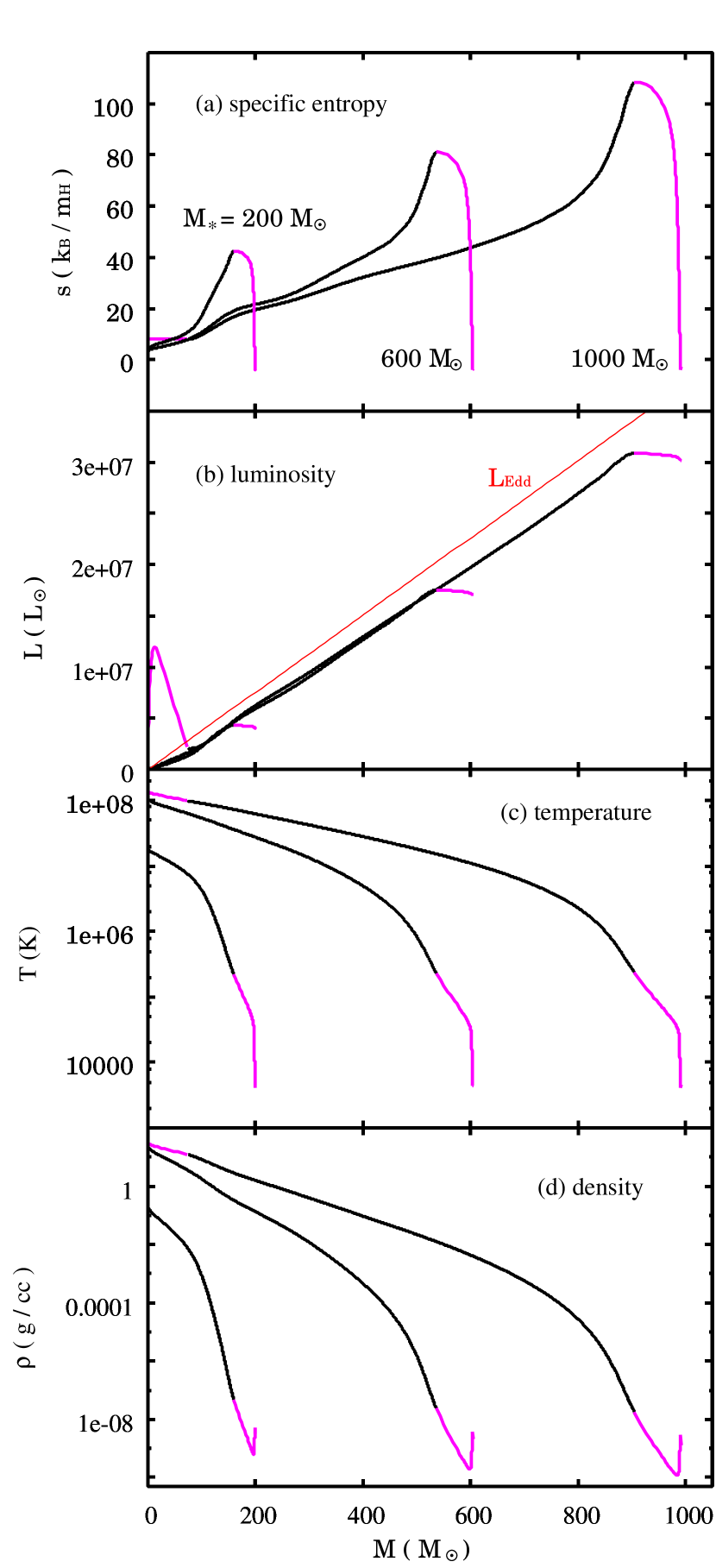
Figure 4.— Radial profiles of the specific entropy (panel a), luminosity (b), temperature (c) and gas mass density (d) in the stellar interior for the fiducial case with $0.1~{}M_{\odot}~{}{\rm yr}^{-1}$ (MD1e1). The profiles when the stellar mass is $200~{}M_{\odot}$, $600~{}M_{\odot}$, and $10^{3}~{}M_{\odot}$ are shown in each panel. The magenta parts indicate the layers are convective. The thin red line in panel (b) represents the Eddington-limit luminosity as a function of the mass coordinate $M$.

In the outer parts of the star, where temperature and density are lower, however, opacity is higher than in the core because of bound-free absorption of H, He atoms and the H^- ion. Energy transport via radiation is inefficient there, and a part of the energy coming from the core is carried outward via convection. Figure 4 shows that the surface convective layer lies in the temperature and density range where $T\lesssim 10^{5}$ K and $\rho\lesssim 10^{-8}~{}{\rm cm}^{-3}$, which is almost independent of the stellar mass. We also see that the specific entropy is not constant over the convective layer, decreasing toward the stellar surface (a so-called super-adiabatic layer). This is because convective heat transport is inefficient near the stellar surface. A part of the outflowing energy is absorbed there, as indicated by the fact that the surface layer has a negative luminosity gradient $(\partial L/\partial M)_{t}<0$. This explains the high specific entropy in the outer convective layer.

The outermost part of the star has a density inversion, i.e. the density increases toward the stellar surface. Here, opacity assumes very high values because of H^- absorption. Radiation pressure is so strong that the hydrostatic balance is not achieved only with gravity; the additional inward force by the negative gas pressure gradient helps maintain the hydrostatic structure. Note, however, that this density inversion could be unstable in realistic multi-dimensions (see e.g., Begelman et al., 2008).

Although deuterium burning is ignited when the stellar mass is $\simeq 50~{}M_{\odot}$, its influence on the subsequent evolution is negligible (Fig. 1). The total energy production rate by deuterium burning is approximately

$$L_{\rm D,st} \equiv \dot{M}_{*}\delta_{\rm D}$$

$$= 1.5\times 10^{5}~{}L_{\odot}\left(\frac{\dot{M}_{*}}{0.1~{}M_{\odot}~{}{\rm yr}^{-1}}\right)\left(\frac{[{\rm D/H}]}{2.5\times 10^{-5}}\right),$$

where $\delta_{\rm D}$ is the energy available from deuterium burning per unit gas mass. Since this is much lower than the Eddington luminosity $L_{\rm Edd}$ in the mass range considered, energy production by deuterium burning contributes only slightly to the luminosity in the stellar interior. Hosokawa & Omukai (2009) showed that deuterium burning influences the stellar evolution only when the accretion rate is low $\dot{M}_{*}\lesssim 10^{-4}~{}M_{\odot}~{}{\rm yr}^{-1}$.

Figure 4 (c) shows that temperature in the stellar interior increases with total mass. The central temperature reaches $10^{8}$ K when the stellar mass is $\simeq 600~{}M_{\odot}$. Soon after that, hydrogen burning begins and a central convective core develops (Fig. 1). This convective core can also be seen in the radial profiles for the $10^{3}~{}M_{\odot}$ model in Figure 4 (indicated by magenta). The luminosity profile tells that most of the energy produced by hydrogen burning is absorbed within the convective core. The star still shines largely by releasing its gravitational energy even after hydrogen ignition.

When the stellar radius is sufficiently large, the accretion flow reaches the stellar surface before becoming opaque to the outgoing stellar light. In fact, soon after the end of the adiabatic accretion stage, the accreting envelope remains optically thin throughout (Fig. 3 c). We also see that the stellar effective temperature is almost constant at $T_{\rm eff}\simeq 5000$ K during this period. In general, the stellar effective temperature never assumes a lower value due to the strong temperature-dependence of H^- absorption opacity (e.g., Hayashi, 1961). Stars that have a compact core and bloated envelope (e.g., red giants) commonly have an almost constant effective temperature, regardless of their stellar masses.

3.2. Cases with Different Accretion Rates

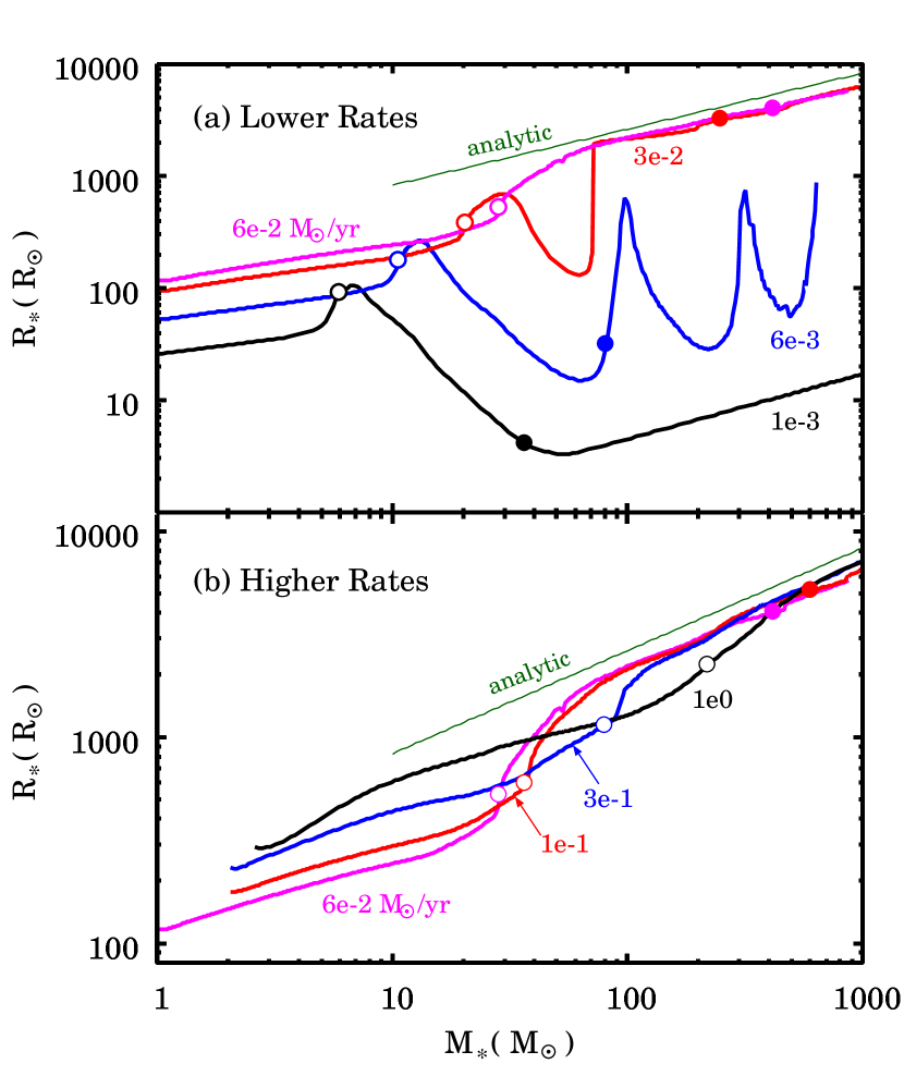
Figure 5.— Evolution of the protostellar radius for various accretion rates. Upper panel: the different curves represent the cases with $\dot{M}_{*}=10^{-3}~{}M_{\odot}~{}{\rm yr}^{-1}$ (case MD1e3, black), $6\times 10^{-3}~{}M_{\odot}~{}{\rm yr}^{-1}$ (MD6e3, blue), $3\times 10^{-2}~{}M_{\odot}~{}{\rm yr}^{-1}$ (MD3e2, red), and $6\times 10^{-2}~{}M_{\odot}~{}{\rm yr}^{-1}$ (MD6e2, magenta). The open and filled circles on each curve denote the epoch when $t_{\rm KH}=t_{\rm acc}$ and when the central hydrogen burning begins, respectively. Lower panel: same as the upper panel but for higher accretion rates of $6\times 10^{-2}~{}M_{\odot}~{}{\rm yr}^{-1}$ (MD6e2, magenta), $0.1~{}M_{\odot}~{}{\rm yr}^{-1}$ (MD1e1, red), $0.3~{}M_{\odot}~{}{\rm yr}^{-1}$ (MD3e1, blue), and $1~{}M_{\odot}~{}{\rm yr}^{-1}$ (MD1e0, black). The case MDe2 is illustrated in both panels as a reference. For the cases with $0.3~{}M_{\odot}~{}{\rm yr}^{-1}$ and $1~{}M_{\odot}~{}{\rm yr}^{-1}$ (MD3e1 and MD1e0) hydrogen fusion has not ignited by the time the stellar mass reaches $10^{3}~{}M_{\odot}$. In the both panels the thin green line represents the mass-radius relation given by equation (12).

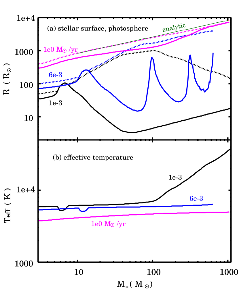
Figure 6.— Upper panel: Evolution of radial positions of the stellar surface (solid) and photosphere (dotted). The black, blue, and magenta curves denote cases with $\dot{M}_{*}=10^{-3}~{}M_{\odot}~{}{\rm yr}^{-1}$ (case MD1e3), $6\times 10^{-3}~{}M_{\odot}~{}{\rm yr}^{-1}$ (MD6e3), and $1~{}M_{\odot}~{}{\rm yr}^{-1}$ (MD1e0), respectively. The mass-radius relation given by equation (12) is plotted with the thin green line. Lower panel: The stellar effective temperature for the same cases as in the upper panel.

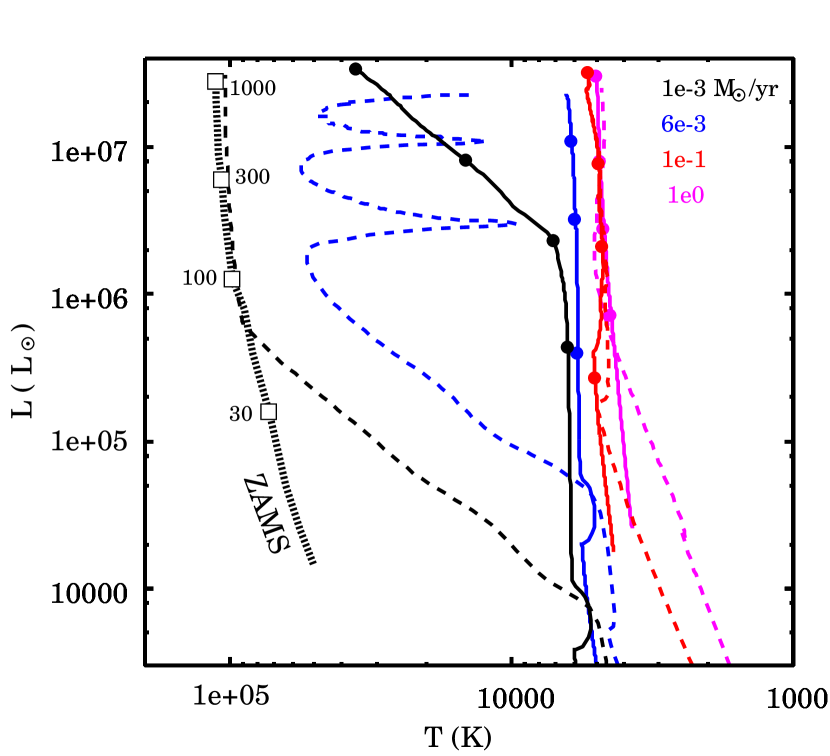
Figure 7.— Evolutionary tracks in the HR diagram. The different colors denote the evolution for different accretion rates, $10^{-3}~{}M_{\odot}~{}{\rm yr}^{-1}$ (case MD1e3, black), $6\times 10^{-3}~{}M_{\odot}~{}{\rm yr}^{-1}$ (MD6e3, blue), $0.1~{}M_{\odot}~{}{\rm yr}^{-1}$ (MD1e1, red), $1~{}M_{\odot}~{}{\rm yr}^{-1}$ (MD1e0, magenta). For each case the values at the stellar photosphere ($L_{\rm tot}$ and $T_{\rm eff}$) and at the stellar surface ($L_{*}$ and $T_{\rm eff,*}\equiv L_{*}/4\pi\sigma R_{*}^{2}$) are plotted with solid and dashed lines, respectively. The thick dashed line represents the loci of non-accreting ZAMS stars taken from Marigo et al. (2001) ($M_{*}\leq 100~{}M_{\odot}$) and Bromm et al. (2001) ($M_{*}\geq 100~{}M_{\odot}$). The filled circles and open squares on the lines mark the positions for $M_{*}=30~{}M_{\odot}$, $100~{}M_{\odot}$, $300~{}M_{\odot}$, and $10^{3}~{}M_{\odot}$ in ascending order.

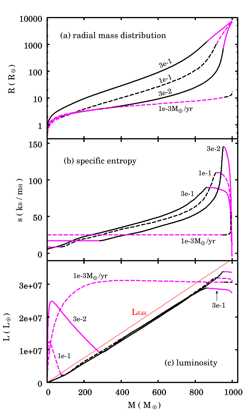
Figure 8.— Comparisons of the interior structure of $10^{3}~{}M_{\odot}$ stars produced by different accretion rates. Radial profiles of mass (panel a), specific entropy (b), and luminosity (c) are shown. In each panel the solid and dashed curves represent the cases for $0.3~{}M_{\odot}~{}{\rm yr}^{-1}$ (MD3e1), $0.1~{}M_{\odot}~{}{\rm yr}^{-1}$ (MD1e1), $3\times 10^{-2}~{}M_{\odot}~{}{\rm yr}^{-1}$ (MD3e2), and $10^{-3}~{}M_{\odot}~{}{\rm yr}^{-1}$ (MD1e3). The magenta lines mark convective layers in the stellar interior. The thin red line in panel (c) represents the Eddington luminosity as a function of mass $M$.

We now investigate how stellar evolution changes with the accretion rate. Figure 5 shows the evolution of the stellar radius for several cases, including $\dot{M}_{*}=10^{-3}~{}M_{\odot}~{}{\rm yr}^{-1}$ (case MD1e3) and $0.1~{}M_{\odot}~{}{\rm yr}^{-1}$ (case MD1e1) explained in Section 3.1. We see that, with accretion rates higher than $6\times 10^{-2}~{}M_{\odot}~{}{\rm yr}^{-1}$, the evolution becomes similar to that of the fiducial case for $0.1~{}M_{\odot}~{}{\rm yr}^{-1}$ (MD1e1); the stellar radius monotonically increases with mass. The protostars undergo adiabatic accretion in the early stage. As equation (6) shows, the stellar radius is larger for higher accretion rates at a given stellar mass, say, at $M_{*}=10~{}M_{\odot}$.

Adiabatic accretion occurs up to a higher stellar mass when the accretion rate is higher. We derive an analytic expression describing this dependence in the following. As long as the KH timescale $t_{\rm KH}$ is longer than the accretion timescale $t_{\rm acc}$, we have adiabatic accretion. (e.g., Hosokawa & Omukai, 2009). Figure 2 shows that $L_{\rm max}$, whose evolution is well described by simple analytic expressions (eqs. 3 and 4), converges to $L_{*}$ at the end of the adiabatic accretion stage. Thus, the stellar mass when the adiabatic accretion terminates $M_{\rm*,teq}$ can be estimated with the relation $t_{\rm acc}\simeq t_{\rm KH}=GM_{*}^{2}/R_{*}L_{\rm max}$. Eliminating $L_{\rm max}$ and $R_{*}$ with equations (4) and (6), we obtain

$$M_{\rm*,teq}\simeq 14.9~{}M_{\odot}\left(\frac{\dot{M}_{*}}{10^{-2}~{}M_{\odot}~{}{\rm yr}^{-1}}\right)^{0.26}.$$ (10)

We have confirmed that the epoch of the timescale equality in our numerical calculation is well described by this equation.

Even after $t_{\rm KH}$ becomes shorter than $t_{\rm acc}$, the stellar radius continues to increase for accretion rates $\gtrsim 10^{-2}~{}M_{\odot}~{}{\rm yr}^{-1}$. The variations of radii among cases with different accretion rates gradually disappear. The stellar radii finally converge to a unique mass-radius relation with $R_{*}\propto M_{*}^{1/2}$ in all the cases. We can derive the approximate mass-radius relation from the following simple argument. First, the stellar luminosity is generally written as

$$L_{*}=4\pi R_{*}^{2}\sigma T_{\rm eff}^{4},$$ (11)

where $\sigma$ is the Stefan-Boltzman constant. As Figure 3 indicates, the stellar luminosity approaches the Eddington value $L_{\rm Edd}(M_{*})$ for $M_{*}\gtrsim 100~{}M_{\odot}$. As explained in Section 3.1 the stellar effective temperature stays at the constant value $T_{\rm eff}\simeq 5000$ K after the inversion of the timescales (also see Figs. 6 and 7). Substituting these relations into equation (11), we obtain

$$R_{*}\simeq 2.6\times 10^{3}~{}R_{\odot}\left(\frac{M_{*}}{100~{}M_{\odot}}\right)^{1/2}.$$ (12)

Figure 5 shows that our numerical results approximately follow this relation.

Begelman (2010) also considered stellar evolution with very rapid mass accretion using simple analytic arguments. His model predicts that the stellar radius is proportional to the mass accretion rate (his eq. 24), which does not agree with our numerical results. Begelman (2010), however, does not take into account the detailed structure of the outermost layer of the star, where H^- opacity is important. The fact that the strong $T$-dependence of H^- opacity keeps the stellar effective temperature almost constant is essential for our results.

Cases MD3e2 and MD6e3 model stellar evolution at intermediate accretion rates ($3\times 10^{-2}$ and $6\times 10^{-3}~{}M_{\odot}~{}{\rm yr}^{-1}$, respectively) and exhibit a different behavior than the higher accretion-rate cases described above. For an accretion rate $3\times 10^{-2}~{}M_{\odot}~{}{\rm yr}^{-1}$ (MD3e2) the protostar initially contracts after the adiabatic accretion stage. At $M_{*}\simeq 70~{}M_{\odot}$, however, the stellar radius sharply increases and ultimately converges to the mass-radius relation given by equation (12). The case with $6\times 10^{-3}~{}M_{\odot}~{}{\rm yr}^{-1}$ exhibits an oscillatory behavior of the stellar radius for $M_{*}\gtrsim 70~{}M_{\odot}$. In this case the accreting envelope remains optically thick after the onset of KH contraction (Figs. 6 and 7). Its photospheric radius still follows the mass-radius relation $R_{\rm ph}\propto M_{*}^{1/2}$. The effective temperature also assumes the constant value $T_{\rm eff}\simeq 6000~{}K$. These evolutionary features for $\dot{M}_{*}<10^{-2}~{}M_{\odot}~{}{\rm yr}^{-1}$ have also been found in previous studies (e.g., Omukai & Palla, 2001, 2003).

We have seen that the stellar radius at $M_{*}\simeq 10^{3}~{}M_{\odot}$ is almost independent of accretion rate as long as $\dot{M}_{*}\gtrsim 3\times 10^{-2}~{}M_{\odot}~{}{\rm yr}^{-1}$. However, the stellar interior structure at this moment is not identical among these cases (Fig. 8). Although each of these stars has a radiative core and a convective envelope, the mass is more strongly centrally concentrated for the lower accretion rates; the less massive envelopes have a higher entropy and inflate even more to achieve the same stellar radius.

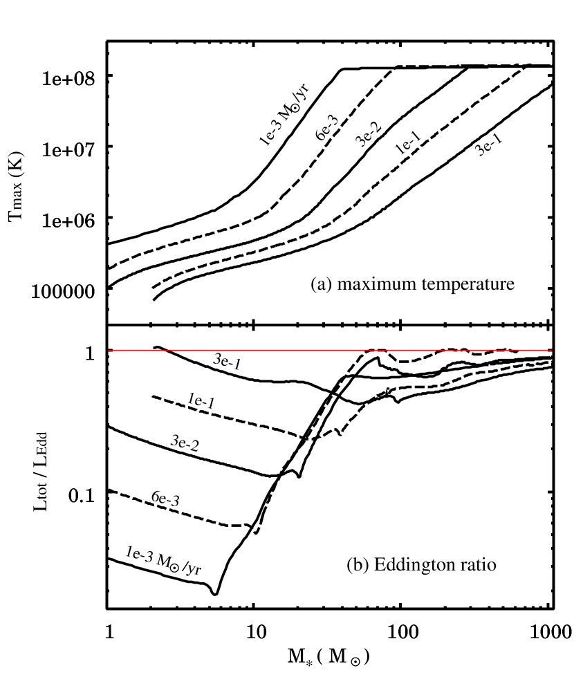
Figure 9.— Evolution of the maximum temperature in the stellar interior (upper panel) and Eddington ratio $L_{\rm tot}/L_{\rm Edd}$ (lower panel) with increasing stellar mass. The solid and dashed curves alternately represent the cases with different accretion rates, $10^{-3}~{}M_{\odot}~{}{\rm yr}^{-1}$ (case MD1e3), $6\times 10^{-3}~{}M_{\odot}~{}{\rm yr}^{-1}$ (MD6e3), $3\times 10^{-2}~{}M_{\odot}~{}{\rm yr}^{-1}$ (MD3e2), $0.1~{}M_{\odot}~{}{\rm yr}^{-1}$ (MD1e1), and $0.3~{}M_{\odot}~{}{\rm yr}^{-1}$ (MD3e1).

The evolution of the stellar maximum temperature is helpful for understanding the variation of the stellar interior structure (Fig. 9 a) with accretion rate. As equation (10) shows, the central part of the star begins to contract and release gravitational energy at a lower stellar mass for the lower accretion rates. The central temperature quickly increases with stellar mass once the KH time becomes shorter than the accretion time. The maximum temperature $T_{\rm max}$ reaches $10^{8}$ K at a lower stellar mass for the lower accretion rate. After that $T_{\rm max}$ assumes an almost constant value due to the strong $T$-dependence of the energy production rate of hydrogen burning. For the case with $3\times 10^{-2}~{}M_{\odot}~{}{\rm yr}^{-1}$ (MD3e2) hydrogen burning begins at $M_{*}\simeq 200~{}M_{\odot}$; the resulting central convective core is seen in the profiles in Figure 8. This feature is not seen for the case with $0.3~{}M_{\odot}~{}{\rm yr}^{-1}$, because hydrogen has not yet ignited by the time $M_{*}=10^{3}~{}M_{\odot}$ for $\dot{M}_{*}\gtrsim 0.3~{}M_{\odot}~{}{\rm yr}^{-1}$.

Figure 5 shows that for $\dot{M}_{*}\gtrsim 6\times 10^{-3}~{}M_{\odot}~{}{\rm yr}^{-1}$ the protostar cannot reach the ZAMS stage by KH contraction. Omukai & Palla (2003) pointed out that this is because the total luminosity $L_{\rm tot}\equiv L_{*}+L_{\rm acc}$ becomes close to the Eddington limit during the contraction to the ZAMS. For the cases with $6\times 10^{-3}$ and $3\times 10^{-2}~{}M_{\odot}~{}{\rm yr}^{-1}$ (cases MD6e3 and MD3e2), for example, the abrupt expansion terminates the KH contraction when the total luminosity is nearly at the Eddington limit (Fig. 9 b). Omukai & Palla (2003) analytically derived the maximum accretion rate $\simeq 4\times 10^{-3}~{}M_{\odot}~{}{\rm yr}^{-1}$ with which the protostar can reach the ZAMS following KH contraction. Figure 5 indicates that there is another critical accretion rate $\simeq 6\times 10^{-2}~{}M_{\odot}~{}{\rm yr}^{-1}$, above which the stellar evolution changes qualitatively; the KH contraction stage disappears entirely at higher rates. This critical rate can also be derived from a similar argument as the one above.

Note that the increase of stellar mass during the KH contraction stage is smaller for the case with $3\times 10^{-2}~{}M_{\odot}~{}{\rm yr}^{-1}$ than with $6\times 10^{-3}~{}M_{\odot}~{}{\rm yr}^{-1}$. Extending this fact for our critical case, the total luminosity would nearly reach the Eddington limit just at the end of the adiabatic accretion stage, i.e., when $t_{\rm KH}\simeq t_{\rm acc}$. Since the opacity in the surface layer is higher than from Thomson scattering during this epoch, having the total luminosity only slightly lower than the Eddington value causes the star to expand. Thus, the condition for the critical case is

$$2L_{\rm max}\simeq C_{\rm Edd}L_{\rm Edd},$$ (13)

where $C_{\rm Edd}$ is a factor less than the unity and we have used the fact that the total luminosity is written as $L_{\rm tot}\simeq 2L_{\rm max}$ when $t_{\rm KH}\simeq t_{\rm acc}$. Using $C_{\rm Edd}=0.25$ as a fiducial value (Fig. 9 b) and equation (4) for $L_{\rm max}$, the stellar mass which satisfies the condition (13) is

$$M_{\rm*,Edd,teq}\simeq 21.7~{}M_{\odot}\left(\frac{C_{\rm Edd}}{0.25}\right)^{0.5}.$$ (14)

On the other hand, equation (10) also gives the stellar mass when $t_{\rm KH}\simeq t_{\rm acc}$ for a given accretion rate. Equating $M_{\rm*,teq}$ and $M_{\rm*.Edd,teq}$ with equations (10) and (14), we obtain the critical mass accretion rate

$$\dot{M}_{\rm cr}\simeq 4.7\times 10^{-2}~{}M_{\odot}~{}{\rm yr}^{-1}\left(\frac{C_{\rm Edd}}{0.25}\right)^{1.9},$$ (15)

which agrees with our numerical results.

3.3. Effects of Lower-Entropy Accretion

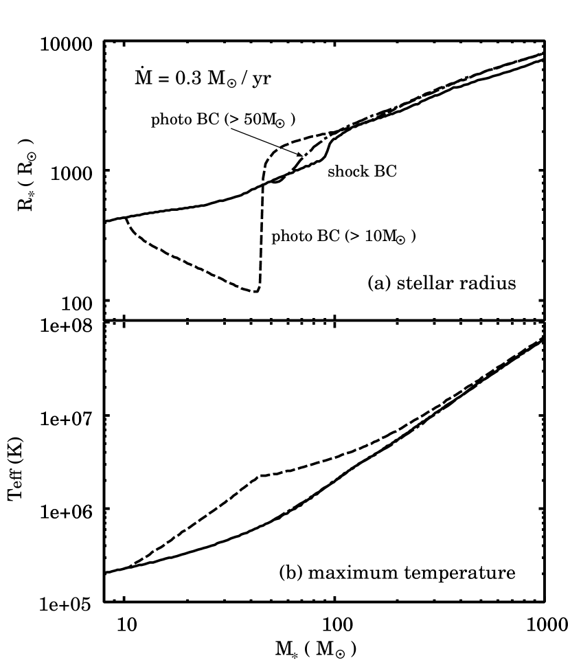
Figure 10.— Effect of reducing the thermal efficiency of mass accretion (upper panel: stellar radius, lower panel: maximum temperature within the star). The same accretion rate of $0.3~{}M_{\odot}~{}{\rm yr}^{-1}$ is adopted for all three cases presented. The solid line represents the evolution with the shock boundary condition, i.e, thermally efficient or “hot” accretion, throughout (MD3e1). The dashed and dot-dashed lines show the evolution in cases MD3e1-HC10 and MD3e1-HC50, where the photospheric boundary condition (i.e., thermally inefficient or “cold” accretion) is adopted after the stellar mass exceeds $10~{}M_{\odot}$ and $50~{}M_{\odot}$, respectively. In the lower panel the dot-dashed line is indistinguishable from the solid line.

We have used the shock outer boundary condition for the stellar models presented and discussed above. As discussed in Section 2.1, the shock boundary condition, which implies that the accreting gas joins the star with relatively high entropy, would be valid for cases with the very rapid mass accretion considered in this paper. If the accred gas had lower entropy, however, the stellar radius would be reduced because of the resulting lower entropy thoughout the stellar interior. Here, we examine potential effects of the colder mass accretion by adopting the photospheric boundary conditions (e.g., Hosokawa et al., 2010, 2011a). Figure 10 (a) shows the evolution of the stellar radius for three cases with $0.3~{}M_{\odot}~{}{\rm yr}^{-1}$, whereby the shock boundary condition is used throughout in one case (MD3e1), whereas the outer boundary condition is changed to the photospheric one for $>10~{}M_{\odot}$ (MD3e1-HCm10) and $>50~{}M_{\odot}$ (MD3e1-HCm50), respectively. The stars are still in the adiabatic accretion stage when the boundary condition is changed in both cases. The different outer boundary conditions do affect the stellar evolution. For the case where the photospheric boundary condition is adopted at $M_{*}=10~{}M_{\odot}$ (MD3e1-HCm10), for example, the star initially contracts after the boundary condition is switched at $M_{*}=10~{}M_{\odot}$, and then abruptly inflates at $M_{*}\simeq 45~{}M_{\odot}$. The stellar radius exceeds $10^{3}~{}R_{\odot}$ and gradually increases with the stellar mass thereafter. In spite of the different behaviors in the early stages, the subsequent evolution for $M_{*}\gtrsim 100~{}M_{\odot}$ is quite similar to that in the case with the shock boundary condition throughout (MD3e1). The evolution when the boundary condition switching occurs at $M_{*}=50~{}M_{\odot}$ (MD3e1-HCm50) is much closer to that in the shock-boundary case. The uniqueness of the mass-radius relation for $M_{*}\gtrsim 100~{}M_{\odot}$ can be explained by the fact that the argument leading to the analytic expression, equation (12), does not assume a specific boundary condition. When the boundary condition is switched at $M_{*}=10~{}M_{\odot}$ (MD3e1-HCm10), the stellar interior temperature is higher and thus the opacity in the stellar interior ($\propto T^{-3.5}$ according to Kramars’s law) is lower than for the shock-boundary case (MD3e1) at the same stellar mass. As a result the star begins to release its internal energy earlier than for the shock-boundary case. Indeed, the timescale equality between $t_{\rm KH}$ and $t_{\rm acc}$ occurs at $M_{*}\simeq 40~{}M_{\odot}$, earlier than for the shock-boundary case, which occurs at the time of abrupt expansion of the stellar radius.

4. Summary and Discussions

We have studied the evolution of stars growing via very rapid mass accretion with $10^{-2}~{}M_{\odot}~{}{\rm yr}^{-1}\lesssim\dot{M}_{*}\lesssim 1~{}M_{\odot}~{}{\rm yr}^{-1}$, which potentially leads to formation of SMBHs in the early universe. In contrast to previous attempts to address this problem, we study the stars’ evolution by numerically solving the stellar structure equations including mass accretion. Our calculations show that stellar evolution in such cases is qualitatively different from that expected for normal Pop III star formation, which proceeds at much lower accretion rates $\sim 10^{-3}-10^{-2}~{}M_{\odot}~{}{\rm yr}^{-1}$. Rapid mass accretion causes the star to inflate; the stellar radius further increases monotonically with stellar mass at least up to $M_{*}\simeq 10^{3}~{}M_{\odot}$. For masses exceeding $\sim 100~{}M_{\odot}$, the star consists of a contracting radiative core and a bloated surface convective layer. The surface layer, which contains only a small fraction of the total stellar mass, fills out most of the stellar radius. The evolution of the stellar radius in this stage follows a unique mass-radius relation $R_{*}\propto M_{*}^{1/2}$, which reaches $\simeq 7000~{}R_{\odot}(\simeq 30$ AU) at $M_{*}=10^{3}~{}M_{\odot}$, in all the cases with $\gtrsim 10^{-2}~{}M_{\odot}~{}{\rm yr}^{-1}$. Hydrogen burning begins only after the star becomes very massive ($M_{*}\gtrsim 100~{}M_{\odot}$); its onset is shifted toward higher masses for higher accretion rates. With very high accretion rates $\dot{M}_{*}\gtrsim 0.1~{}M_{\odot}~{}{\rm yr}^{-1}$, hydrogen is ignited after the stellar mass exceeds $10^{3}~{}M_{\odot}$. The stellar radius continues to grow as $R_{*}\propto M_{*}^{1/2}$ even after hydrogen ignition.

In this paper we have focused on the early evolution until the stellar mass reaches $10^{3}~{}M_{\odot}$. The subsequent evolution remains unexplored because of convergence difficulties with the current numerical codes. If the star continues to expand following the same mass-radius relation (12) also for $M_{*}>10^{3}~{}M_{\odot}$, the stellar radius at $10^{5}~{}M_{\odot}$ would be $\simeq 400$ AU. Since the stellar effective temperature remains $\simeq 5000$ K, the star hardly emits ionizing photons during accretion. Therefore, it is unlikely that stellar growth is limited by the radiative feedback via formation of an HII region as discussed by Hosokawa et al. (2011b). Johnson et al. (2011) also reached an analogous conclusion that UV feedback does not hinder SMS formation. In their argument, however, the star is assumed to reach the ZAMS and to emit a copious amount of ionizing photons, but the expansion of the HII region is squelched by rapid spherical inflow. They also expected that, as a result of confinement of the HII region, strong emission lines reprocessed from the ionizing photons (e.g., Ly $\alpha$ and He II) would escape from the accretion envelope to be an observational signature of these objects. By contrast, our calculations show that the stellar UV luminosity and thus the luminosities in those lines should be much weaker than supposed. Note that the argument by Johnson et al. (2011) assumes perfect spherical symmetry, which allows the HII region to be confined within the accretion envelope. Given that mass accretion will likely occur through a circumstellar disk, the HII region should grow toward the polar region where the gas density is much lower than the spherical accretion flow (e.g., Hosokawa et al., 2011b). This should be the case with the high stellar UV luminosity assumed in Johnson et al. (2011).

Even without stellar radiative feedback, stellar growth via mass accretion might be hindered by some other process, e.g., rapid mass loss. Indeed, evolved massive stars in the Galaxy ($M_{*}\sim 10-100~{}M_{\odot}$), which have large radii ($R_{*}\gtrsim 100~{}R_{\odot}$) and high luminosities close to the Eddington limit ($L_{*}\simeq 10^{6}~{}L_{\odot}$), generally have strong stellar winds with mass losses $\sim 10^{-4}~{}M_{\odot}~{}{\rm yr}^{-1}$ (e.g., Humphreys & Davidson, 1994). Although the line-driven winds of primordial stars are predicted to be weak or non-existent (Krtička & Kubát, 2006), pulsational instability of massive stars has also been found to drive mass loss (Baraffe et al., 2001; Sonoi & Umeda, 2011). Further work is necessary to address how massive SMSs could form via mass accretion in spite of such disruptive effects.

Stellar evolution under conditions of very rapid mass accretion as presented and discussed here is mostly relevant to the formation of stars in the atomic-cooling halos. However, our results could be also important for normal Pop III star formation where H₂ molecular cooling operates. The typical mass accretion rate for this case is around $10^{-3}~{}M_{\odot}~{}{\rm yr}^{-1}$, but in some exceptional situations, e.g., when a progenitor cloud core is extremely slow rotating, higher accretion rates $\dot{M}_{*}\sim 10^{-2}~{}M_{\odot}~{}{\rm yr}^{-1}$ can be realized (e.g., Hosokawa et al., 2011b). Since the stellar effective temperature is low at $\simeq 5000$ K with rapid mass accretion, formation of the HII region would be postponed until the mass accretion rate falls below $10^{-2}~{}M_{\odot}~{}{\rm yr}^{-1}$. This would help the primordial star to grow to more than $100~{}M_{\odot}$ in the molecular-cooling halos (see also Omukai & Palla, 2003).

References

- Alvarez et al. (2009) Alvarez, M. A., Wise, J. H., & Abel, T. 2009, ApJ, 701, L133
- Ball et al. (2011) Ball, W. H., Tout, C. A., Żytkow, A. N., & Eldridge, J. J. 2011, MNRAS, 414, 2751
- Baraffe et al. (2001) Baraffe, I., Heger, A., & Woosley, S. E. 2001, ApJ, 550, 890
- Begelman (2010) Begelman, M. C. 2010, MNRAS, 402, 673
- Begelman et al. (2008) Begelman, M. C., Rossi, E. M., & Armitage, P. J. 2008, MNRAS, 387, 1649
- Begelman et al. (2006) Begelman, M. C., Volonteri, M., & Rees, M. J. 2006, MNRAS, 370, 289
- Bromm et al. (2001) Bromm, V., Kudritzki, R. P., & Loeb, A. 2001, ApJ, 552, 464
- Bromm & Larson (2004) Bromm, V., & Larson, R. B. 2004, ARA&A, 42, 79
- Bromm & Loeb (2003) Bromm, V., & Loeb, A. 2003, ApJ, 596, 34
- Campanelli et al. (2007) Campanelli, M., Lousto, C., Zlochower, Y., & Merritt, D. 2007, ApJ, 659, L5
- Chandrasekhar (1964) Chandrasekhar, S. 1964, Physical Review Letters, 12, 114
- Clark et al. (2011) Clark, P. C., Glover, S. C. O., Smith, R. J., Greif, T. H., Klessen, R. S., & Bromm, V. 2011, Science, 331, 1040
- Dotan et al. (2011) Dotan, C., Rossi, E. M., & Shaviv, N. J. 2011, MNRAS, 417, 3035
- Fan (2006) Fan, X. 2006, New Astron Rev., 50, 665
- Hartmann et al. (1997) Hartmann, L., Cassen, P., & Kenyon, S. J. 1997, ApJ, 475, 770
- Hayashi (1961) Hayashi, C. 1961, PASJ, 13, 450
- Hayashi et al. (1962) Hayashi, C., Hōshi, R., & Sugimoto, D. 1962, Progress of Theoretical Physics Supplement, 22, 1
- Heger & Woosley (2002) Heger, A., & Woosley, S. E. 2002, ApJ, 567, 532
- Herrmann et al. (2007) Herrmann, F., Hinder, I., Shoemaker, D., & Laguna, P. 2007, Classical and Quantum Gravity, 24, 33
- Hosokawa et al. (2011a) Hosokawa, T., Offner, S. S. R., & Krumholz, M. R. 2011a, ApJ, 738, 140
- Hosokawa & Omukai (2009) Hosokawa, T., & Omukai, K. 2009, ApJ, 691, 823
- Hosokawa et al. (2011b) Hosokawa, T., Omukai, K., Yoshida, N., & Yorke, H. W. 2011b, Science, 334, 1250
- Hosokawa et al. (2010) Hosokawa, T., Yorke, H. W., & Omukai, K. 2010, ApJ, 721, 478
- Humphreys & Davidson (1994) Humphreys, R. M., & Davidson, K. 1994, PASP, 106, 1025
- Inayoshi & Omukai (2011) Inayoshi, K., & Omukai, K. 2011, MNRAS, 416, 2748
- Inayoshi & Omukai (2012) —. 2012, ArXiv e-prints:1202.5380
- Jeon et al. (2011) Jeon, M., Pawlik, A. H., Greif, T. H., Glover, S. C. O., Bromm, V., Milosavljevic, M., & Klessen, R. S. 2011, ArXiv e-prints:1111.6305
- Johnson et al. (2011) Johnson, J. L., Whalen, D. J., Fryer, C. L., & Li, H. 2011, ArXiv e-prints:1112.2726
- Kitayama & Yoshida (2005) Kitayama, T., & Yoshida, N. 2005, ApJ, 630, 675
- Kitayama et al. (2004) Kitayama, T., Yoshida, N., Susa, H., & Umemura, M. 2004, ApJ, 613, 631
- Krtička & Kubát (2006) Krtička, J., & Kubát, J. 2006, A&A, 446, 1039
- Machida et al. (2008) Machida, M. N., Omukai, K., Matsumoto, T., & Inutsuka, S.-i. 2008, ApJ, 677, 813
- Madau & Rees (2001) Madau, P., & Rees, M. J. 2001, ApJ, 551, L27
- Marigo et al. (2001) Marigo, P., Girardi, L., Chiosi, C., & Wood, P. R. 2001, A&A, 371, 152
- McKee & Tan (2008) McKee, C. F., & Tan, J. C. 2008, ApJ, 681, 771
- Milosavljević et al. (2009) Milosavljević, M., Couch, S. M., & Bromm, V. 2009, ApJ, 696, L146
- Mortlock et al. (2011) Mortlock, D. J., et al. 2011, Nature, 474, 616
- Oh & Haiman (2002) Oh, S. P., & Haiman, Z. 2002, ApJ, 569, 558
- Ohkubo et al. (2009) Ohkubo, T., Nomoto, K., Umeda, H., Yoshida, N., & Tsuruta, S. 2009, ApJ, 706, 1184
- Omukai (2001) Omukai, K. 2001, ApJ, 546, 635
- Omukai & Palla (2001) Omukai, K., & Palla, F. 2001, ApJ, 561, L55
- Omukai & Palla (2003) —. 2003, ApJ, 589, 677
- Palla & Stahler (1992) Palla, F., & Stahler, S. W. 1992, ApJ, 392, 667
- Popham et al. (1993) Popham, R., Narayan, R., Hartmann, L., & Kenyon, S. 1993, ApJ, 415, L127
- Regan & Haehnelt (2009) Regan, J. A., & Haehnelt, M. G. 2009, MNRAS, 393, 858
- Schneider et al. (2002) Schneider, R., Ferrara, A., Natarajan, P., & Omukai, K. 2002, ApJ, 571, 30
- Shang et al. (2010) Shang, C., Bryan, G. L., & Haiman, Z. 2010, MNRAS, 402, 1249
- Shibata & Shapiro (2002) Shibata, M., & Shapiro, S. L. 2002, ApJ, 572, L39
- Smith et al. (2011) Smith, R. J., Hosokawa, T., Omukai, K., Glover, S. C. O., & Klessen, R. S. 2011, ArXiv e-prints:1112.4157
- Sonoi & Umeda (2011) Sonoi, T., & Umeda, H. 2011, MNRAS, L389
- Stacy et al. (2010) Stacy, A., Greif, T. H., & Bromm, V. 2010, MNRAS, 403, 45
- Stacy et al. (2012) —. 2012, MNRAS, 2508
- Stahler et al. (1986) Stahler, S. W., Palla, F., & Salpeter, E. E. 1986, ApJ, 302, 590
- Stahler et al. (1980) Stahler, S. W., Shu, F. H., & Taam, R. E. 1980, ApJ, 241, 637
- Treister et al. (2011) Treister, E., Schawinski, K., Volonteri, M., Natarajan, P., & Gawiser, E. 2011, Nature, 474, 356
- Whalen et al. (2004) Whalen, D., Abel, T., & Norman, M. L. 2004, ApJ, 610, 14