Evolutionary Rotation in Switching Incentive Zero-Sum Games

Abstract

In a competitive game situation where the only Nash equilibrium is in mixed strategies, persistent cyclic social rotation can be expected. The rotation is pointed out firstly by Shapley (1964) as never-ending cycle and in discrete condition called as Shapley-ploygon. To insight into the rotation is long time expectation. Data comes from an 13 groups, 825 rounds and 7 games experiment, which are of random matching two-persons zero-sum extended 2$\times$2 games (Binmore, Swierzbinski and Proulx, 2001 Binmore et al. (2001)). Whenever the payoff matrix is switched by the experimenters, we find, the human subjects social rotations’ directions and strengths is changed simultaneously. The directions of rotation can be captured by evolutionary dynamics; meanwhile, an explanation for observed rotation strengths is also given with eigenvalues calculated from the Jacobian of normalized replicator dynamics. In addition, equality-of-populations rank test shows that relative response coefficients within groups differ and persist cross the parameters switching. In the old data, we demonstrate a new view — rotation — to insight the Shapley-cyclic motion strength quantitatively.

I 1. Introduction

In theoretical economic history, Shapley’s the never-ending cycle in game (Shapley, 1964), as the Edgeworth cycle in price (Edgeworth, 1925), is a deep insight into stochastic processes of social evolution Benaīm et al. (2009). Shapley never-ending cycle (now called as Shapley-polygon) state that, in a competitive situation where the only Nash equilibrium is in mixed strategies, persistent cycles can be expected Benaīm et al. (2009). The unstable equilibrium has been strongly linking to evolutionary game theory (EGT) and learning processes Gaunersdorfer and Hofbauer (1995); Benaīm et al. (2009); Cason et al. (2010) in the past decades.

Experimental economics can be a method for theory testing Falk and Heckman (2009); Samuelson (2002). To the best of our knowledge, the Shapley-polygon has rare been well experimental tested. Only closing experimental literature comes from Cason, Friedman and Hopkins Cason et al. (2010). The strength of rotation of Shapley-polygon has never been reported. In this letter, in old experimental data of zero-sums games Binmore et al. (2001), we report that, not only the direction, but also the strength of social rotation can be distinguished, and even more, quantitatively, the results support the predictions from Shapley-polygon and EGT.

This report starts from the Binmore, Swierzbinski and Proulx’s experiment Binmore et al. (2001). The experiment is repeated in 13 groups. Each group contains 12 human subjects which are split into two populations to play random matching two-person companion 2$\times$2 games. Interesting is that, there are exists 7 different incentives (payoff matrix) along the 825 rounds game, or, the incentives parameter changes 6 times along the 825 periods (see Figure 1). This switching parameters experiment provides us a chance to insight (1) the changing direction and strength of social cyclic motions, and even more, (2) the inherence (relative dynamical response coefficient) of the social groups’ dynamic property, quantitatively.

After introducing the measurement method and the experiment in section 2, in section 3 we show that (1) not only the direction but also the strength of the social rotation can be quantitatively distinguished; and (2) the diversity of the response coefficient cross the groups can be distinguished. In section 4, a potential theoretical explanation linking the strength of rotation to the payoff matrix is provided quantitatively, and then, discuss and summary last.

———————————————————————————————————————————————————
(a)
———————————————————————————————————————————————————

———————————————————————————————————————————————————
(b)
———————————————————————————————————————————————————

———————————————————————————————————————————————————
(c)
———————————————————————————————————————————————————

0              -              +              0             +             -               -                             
———————————————————————————————————————————————————
(d)
———————————————————————————————————————————————————

Figure 1: Illustration of the Experiments. Each of the 13 groups ($\beta=1,2,...,13$) play 7 games ($\alpha=1,2,...,7$) and 825 periods total. (a) From left to right, the matrix are the payoff matrix of the 7 games along total 825 experimental rounds (time, $t$). Time arrows indicate the duration of the games. (b) From left to right, matrix are the companion 2$\times$2 games to each of games Binmore et al. (2001). (c) Phase diagrams for the replicator dynamics of above companion 2$\times$2 payoff matrix, the theoretical expected direction of the social rotation. Arrows in black lines indicate the direction of trajectories of the evolution. Figure is made by the game dynamics program Dynamo Sandholm (2011). The positive (+) symbol indicate the expected evolutionary direction is counterclockwise, negative (-) is clockwise and zero (0) means no rotation. (d) The accumulate rotation $L^{a}$ of each of the 13 groups and initial by the 7 games respectively. The eigenvalue (calculation see text) for each game plotted in dash line in each game duration. Insert (right-up): Theoretical expected values $\lambda$ (includes the direction and the eigenvalue of the Jacobian) and the experimental mean rotation $\bar{L}$ (by rounds) values for the 5 real games in fulled dot, labeled with $\alpha$ (game ID).

II 2. Measurement and Data

As a dynamics model, EGT offers short run predictions where classic game theory has little to say. Quantitative, in the 2$\times$2-like MSNE games Binmore et al. (2001), EGT predicts the evolution cyclic trajectory and rotation globally. To capture the rotation, quantitatively, is the main propose of this paper. The measurement for the rotation is introduced following.

II.1 Strategy Space and Social Evolution

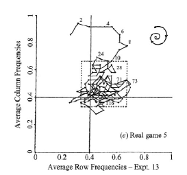
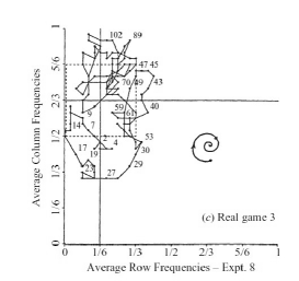
For simple and clarity, we start from two-dimensional state space for two-population random matching two-persons 2$\times$2 games. In EGT analogy Sandholm (2011), social output can be described by the state space, the states and time. In the game, there exists two roles and each role includes some agents. For the first population $X$, the strategy set is $\{X_{1}$,$X_{2}\}$ for each agent; similarly, for the second population $Y$, $\{Y_{1}$,$Y_{2}\}$. Numerically, as ref. Selten and Chmura (2008), we denote the strategy of $X_{1}$ (up strategy) and $Y_{1}$ (left strategy) as 1 following. The payoff matrix, as an example, is shown in Fig. 1(b). For a given the payoff matrix, the solution of an evolutionary dynamics model can be seen in Fig. 1(c) Schuster and Sigmund (1981) and two experimental trajectories can be seen in Fig. 2(b) Binmore et al. (2001). If there are $N$=6 agents in each population, an observable instantaneous populations strategy state should be $x$:=$(p,q)\in\mathbb{X}$, herein $\mathbb{X}$ is the populations strategy state space and $\mathbb{X}$=$\{0,\frac{1}{6},\frac{2}{6},\ldots,1\}\times\{0,\frac{1}{6},\frac{2}{6},\ldots,1\}$, and $p$ ($q$) is the density of $X_{1}$ ($Y_{1}$) in $X$ ($Y$). The strategy space is always an unit square.

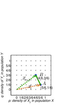
Figure 2(c) is an illustration for the state space of a 6+6 two-population 2$\times$2 game. The unit square $7\times 7$ lattice (gray dots) is the state space $\mathbb{X}$; In Fig. 2(a), $A$ is the $x_{A}$=($\frac{5}{6},\frac{1}{6}$) is a state which means that $\frac{5}{6}$ in population $X$ choice $X_{1}$ meanwhile $\frac{1}{6}$ in population $Y$ choice $Y_{1}$.

In an experimental economics session, at each round, $t$, there is one dot of observation of $x(t)$ in $\mathbb{X}$. The vector, $x(t)$, is an indicator of collective social behavior at $t$. The smallest tick $\triangle t$ is $1$ and is the interval within the successive two rounds. Round by round, the dot ($x(t)$) should jump in the lattice and should form a trajectory. Figure 2(b) is an empirical example of a trajectory. The experimental system can be seen as a discrete-space and discrete-time population dynamics system.

We investigate social dynamics in existed experimental data. Qualitatively, the authors Binmore et al. (2001) confirm that, in the trajectories in some sessions, as expected by evolutionary game theory or as Shapley (1964) cycle prediction, motion spiral pattern exists. We go one step ahead. Quantitatively, we find the strength of the social motion spiral can be distinguished and fit evolutionary game theory better than ever known.

II.2 Measurement for Rotation

We are interested in the rotation observable – a vector ($L$) called as rotation – an indicator for the direction and the strength of the social evolutionary motion (or say as, the collective social dynamic behavior). In a two-population random matching two-persons 2$\times$2 game, $L$ can be seen as a one-dimensional vector perpendicular to the two-dimensional state space.

At experimental round $t$, the instantaneous rotation $L(t)$ can be expressed as

$$L(t) = x(t)\otimes x(t+1),$$ (1)

where $x(t)$ is the strategy vector at time $t$, the $\otimes$ is cross product within the two strategy vectors. An example of an instantaneous rotation $L(t)$ is shown in Fig. 2(a). Denoting $T$ as the total number of rounds in game ($\alpha$) in group ($\beta$), the accumulated $L$ (denoted as $L^{a}$) is $L_{\alpha,\beta}^{a}=\sum_{t=0}^{T-1}\!L(t)$ in which $T$ is the total periods of the game $\alpha$ of the human subjects group $\beta$. The mean instantaneous rotation can be denoted as $\bar{L}_{\alpha,\beta}=L_{\alpha,\beta}^{a}/T$. A simplest picture is, $\bar{L}_{\alpha,\beta}$ should depend on both $\alpha$ (an exogenous incentive of the experimental parameter setting) and $\beta$ (the inherence of a social group). If $\bar{L}_{\alpha,\beta}>0$, the rotation is counterclockwise; alternatively, clockwise.

We briefly explain the rotation observable $\bar{L}_{\alpha,\beta}$ here. Given same $\alpha$, if $\bar{L}_{.,\beta}\neq\bar{L}_{.,\beta^{\prime}}$, we can say, the ”social material” $\beta$ is unequal to $\beta^{\prime}$, or say, the response coefficients of the materials differ. Meanwhile, given same $\beta$, changing $\alpha$ is changing incentive, and then, the strength of rotation should be changed. In statistical physics language, $\bar{L}$ relates to probability current or flux in state space. This observable relates Shapley polygon Shapley (1964) and stability of social dynamics (e.g., Cason et al. (2010)). This observable can also be imaged as angular momentum, one of the most fundamental variable in physics, but set mass term as 1.

———————————————————————————————————————————————————
(a)                                                              (b)                   
———————————————————————————————————————————————————

Figure 2: Measurement of the Social Rotation in State Space. (a) Illustration of an instantaneous social rotation $L$ at time $t$. Supposing at time $t$, $x_{t}$ is at $A(5/6,1/6)$ and the next moment $t+1$, $x(t+1)$ is at $B(4/6,3/6)$; In this jumping from A to B, $L(t)$:=$x(t)\otimes x(t+1)$ is equal to 11/36. If a jumping was from B to A, its $L=-11/36$. Except the last round, every round has its observation of $L$. (b) The trajectory of the social evolution in game 7 (or 5$th$ real game) and game 5 (or the 3$rd$ real game) in the experiment Binmore et al. (2001). The two figures are reproduced from ref. Binmore et al. (2001); Theoretically, spiral in left-hand-side should be clockwise and in right-hand-side should be counterclockwise.

II.3 Data from Switching Parameter Experiments

The controlled parameters in experimental games are of the payoff matrix. The original payoff matrix can be seen in Figure 1(a) in which the row players’s payoff is given; the column player’s payoff is its opposite value; all of the games are of zero-sum game. Figure 1(b) are the zero-sum payoff matrix of the companion 2$\times$2 games in Figure 1(a) Binmore et al. (2001).

The random matching two-persons pair comes from the two populations respectively. The total length of a groups playing is of 825 rounds, with 13 groups containing 12 human subjects. The 12 human subjects are split into two-population equally in which one population play $X$-role and another population play $Y$-role. Each group plays all 7 games in the 825 rounds. The Game 1 and Game 2 are practice zero-sum game and not real game are provided to the human subjects for training. All of the 156 subjects comes from student subject pool in University of Michigan, U.S. The experiments are conducted in the end of 1990s. For more detail of the parameters of the 7 experimental games, see ref. Binmore et al. (2001)

III results

III.1 Gross Figural and Numerical Results

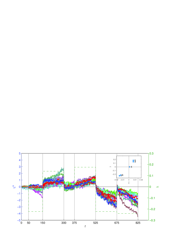
Figure 1(d), the 13 color curves are the empirical accumulate rotation $L^{a}$ of each of the 13 groups and initial by the 7 games respectively. The successive increasing or declining of the $L^{a}$ means the successively counterclockwise or clockwise rotation is observed. Numerical results see Table 1. In these data, (1) in the game dimension, we explore the consequence of the switching the payoff matrix; (2) in the human subject groups dimension, we explore the inherence response coefficient cross the groups.

Table 1: Empirical Accumulate Rotation ($L^{a}$) of the 13 Groups in the 7 Games

Group$(\beta)$	1	2	3	4	5	6	7	8	9	10	11	12	13
Game($\alpha$)	T61	T62	T63	T64	T65	T66	T67	T68	T70	T71	T72	T73	T74	Avg.	S.E.
1	-0.11	0.11	0.03	0.06	-0.14	0.14	-0.44	0.11	0.00	0.03	-0.19	0.03	-0.17	-0.04	0.16
2	-1.69	-0.81	-0.36	-0.56	-0.33	-0.5	-0.33	-0.56	-0.92	-0.14	-0.03	0.11	0.17	-0.46	0.49
3	0.89	0.67	1.47	1.89	0.78	0.81	1.17	0.39	2.53	0.72	0.97	0.72	0.89	1.07	0.58
4	0.39	-0.42	0.14	-0.17	0.56	0.14	0.36	-0.39	0.19	-0.22	0.17	0.17	0.03	0.07	0.3
5	1.25	0.86	1.03	0.94	1.11	1.14	1.58	0.53	1.39	1.72	0.44	1.31	0.61	1.07	0.39
6	-1.47	-0.92	-2.33	-1.5	-1.06	-1.25	-1.53	-2.5	-2.75	-3.06	-2.03	-2.42	-2.69	-1.96	0.71
7	-3.00	-1.31	-1.92	-2.97	-0.94	-2.61	-1.75	-1.36	-2.67	-4.33	-2.47	-1.78	-2.47	-2.28	0.9
R.R.C.	1.02	0.62	1.09	1.18	0.68	0.9	1.03	0.68	1.56	1.44	0.86	0.98	0.97	1	0.28

R.R.C. is the abbreviation of relative response coefficient ($\Phi_{.,\beta}$) of each of the 13 human subject groups. The last row is the mean $\Phi_{.,\beta}$ cross the game $\alpha=3,5,6,7$. The second row (e.g., T61 to T74) is the labeled according to the session order of original experimental record in which there is not session labeled as 69. The mean instantaneous rotation $\bar{L}=L^{a}/T$ in which $T$ is the total round of an experimental session of a given payoff matrix.

———————————————————————————————————————————————————
                   (a)                                                                    (b)                   
———————————————————————————————————————————————————

    

Figure 3: Empirical results. (a) Figural presentation for Result-1.1 and Result-1.2. The box-plot of the mean rotation $\bar{L}_{\alpha,.}$ by Games ($\alpha=1,2,...,7$), in which Groups ($\beta=1,2,...,13$) results are pooled by the 7 games (Result 1.1 and 1.2 in text). (b) Figural presentation for Result-2.1 and Result-2.2. Empirical Result by Groups. The box-plot of the relatively strength $\Phi_{.,\beta}$. From left to right are Group 61-68 and Group 70-74. Each group $\beta$ has 4 samples from Game 3, 5, 6 and 7. A box is the 4 values’ range of $\Phi_{\alpha,.}$ for a given $\beta$ (From left to right, $\beta=1,2,...,13$).

III.2 Cross the 4 MSNE Games: Rotation Strength and Incentive

Theoretically, payoff matrix relates to the incentive of the individual in an experimental social. It is straight to image that, payoff matrix could be links to the strength of social rotation. Different game with different payoff matrix could have different strength of social rotation.

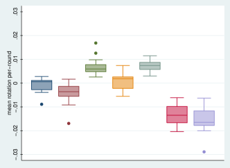
Numerical results of the accumulated rotation of the 13 Groups in the 7 Games are shown in Table 1. Figure 3(a) are the figural results. Both show the direction (positive is along counter-clock) and the strength of the $L^{a}_{\alpha,\beta}$, respectively. From Table 1, row by row’s or game by game’s statistical analysis comes to following two results.

Result-1.1: Numerical analysis show that, the direction in the four games (each with 13 samples) are consistence with evolutionary game theory expectations, respectively ($p<0.00$). None of the 52 samples deviate the theoretical prediction.

Result-1.2: Numerical analysis also show that, the absolutely value of the strength cross the 4 MSNE games can be distinguished. Disregards the direction, numerical results shows that, rotation strength values of both of the Game 6 and Game 7 significant larger than those of the Game 3 and Game 5 ($p<0.01,t$-$test$).

A potential interpretation for the strengths cross the games is given in next section.

III.3 Cross the 13 Human Subjects Groups: Diversity of Response Coefficient

For individual, the sensitive on the incentive could be different and can be detected in game Hsu et al. (2007); Xu and Wang (2011a); For group, the sensitives are different and detectable Camerer and Foundation (2003). The diversity of response character be obtained from the observable – the strength of social rotation.

Within Groups, there is 4 games taken into account to test the diversity on response. We do not include the Game 4, for it is not the MSNE, the observable of rotation is trivial. From Table 1, column by column’s (group by group’s) statistical analysis comes to the results: Result-2.1 and Result-2.2.

Result-2.1: Result-2.1: In the direction of rotation view, none of the 52 (13 group and the 4 games) observed $L^{a}$ deviates the prediction from the evolutionary game theory. The prediction of the replicator dynamics (the most simple EGT model) for the 4 games are shown in Figure 1(c).

None of the groups deviating from EGT’s prediction. This means, in the 12 subjects systems, the social rotation (and also Shapley-cyclic motion) directions obey the EGT. In this view, the similarity between the groups is significant.

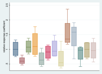
Result-2.2: In the sensitive of the groups response in rotation view, from Table 1, Figure 3(b) are the figural results for the relative accumulated rotation $\Phi_{\alpha,\beta}$ ($\Phi_{\alpha,\beta}=L_{\alpha,\beta}^{a}/L^{\prime}_{\alpha}$, here, $L^{\prime}_{\alpha}=\sum_{\beta}\frac{L_{\alpha,\beta}^{a}}{S_{\beta}}$ and sample size $S_{\beta}=13$ in our case) cross the 13 groups and each group has 4 ($\alpha=3,5,6,7$) samples, respectively. That is to say, for given $\beta$, if $\Phi_{\alpha,\beta}$ is strictly larger than 1, this suggests that, the sample $\beta$ is more sensitive. $\Phi_{\alpha,\beta}$ can be a quantity relating to response coefficient of group $\beta$. Cross the games ($\alpha=3,5,6,7$), the relative accumulated rotation $\Phi_{.,\beta}$ of $\beta$-group is shown in last row Table 1.

We use Kruskal-Wallis equality-of-populations rank test method to evaluate the groups’ response coefficient. Each of the 13 groups is used as a group sample; in each group sample, there is 4 MSNE games’s relative rotation strength observation.

Result shows that, the equality hypothesis can be rejected ( $p<0.05$, $\chi^{2}$=21.330 and 12 degrees of freedom). This result means the different is not random result of the 13 samples. The groups’ inherence (response coefficient) is different and could be persisted cross the games.

Some samples results are: the group 62, 65 and 68 is less ($\Phi_{\alpha,\beta}<$ 1 at $p<0.1$ significant) sensitive to the incentives; Alternatively, the group 70 is the most sensitive ($\Phi_{\alpha,\beta}>$ 1 at $p<0.01$ significant) to the payoff matrix switching. The numeric results of the relative response coefficients (R.R.C.) can be read from the last row in Table 1.

IV A Theoretical Explanation for the Rotation

Trying to find out the theoretical explantation of the strength, we start from the simplest evolutionary dynamical equation – replicate dynamics equation specified by the 2$\times$2 payoff matrix for the two population games. Symbols in this section is following reference Schuster and Sigmund (1981).

On the direction of rotation. Figure 1(c) provides all 7 games pattern with the Dynamo Sandholm (2011). In direction view, all of the results from real experiment (in Game 3, 5, 6 and 7) total 52 sessions meet the theoretical model exactly ($p<0.00$). In Game 4, cross the 13 sample, 13 samples statistically not deviate from zero hypothesis ($t$-$test>$0.1) which is expected by EGT, because, in these systems, no rotation exists.

On the strength of rotation. Theoretically, eigenvalues of the payoff matrix determine the dynamics property like convergence and stability (e.g., Selten (1991)). This point is supported in experiments (e.g., Tang (2001)). Each 2$\times$2 payoff bi-matrix can be simplified to the two matrix

$\left(\begin{array}[]{cc}0&a\\ b&0\\ \end{array}\right)$ and $\left(\begin{array}[]{cc}0&c\\ d&0\\ \end{array}\right)$

as reference Schuster and Sigmund (1981). Then, the two matrix are multiply to satisfied the concentrations:

$$|a+b|=1~{}~{}\cap~{}~{}|c+d|=1,$$ (2)

And the efficient payoff matrix can be obtained. As mentioned in Schuster and Sigmund (1981), there exists an unique equilibrium ($|c|,|a|$) in the interior space if and only if $ab>0$ and $cd>0$ (Game 2, 3, 5, 6 and 7 are in this condition). If not this condition, the dynamic equation is trivial (Game 1 and 4, the systems are not oscillating but converging to pure Nash states). In $ac<0$ case, what is interested in this report, the eigenvalues $v$ of the Jacobian of the dynamic equation evaluated near the unique equilibrium point can be expressed as Schuster and Sigmund (1981),

$$v=\pm i\lambda=\pm i\sqrt{abcd}.$$ (3)

Table 2 is the results along above steps and shows the efficient payoff matrix elements ($a,b,c,d$). Table 2 also shows the eigenvalues ($\lambda$) from Jacobian of replicator dynamics model of the given games. It is well known that the eigenvalue $\lambda$ direct proportion to the frequency (or angular velocity) of vibration; meanwhile, empirically Xu and Wang (2012a), mean $L$ proportion to mean angular velocity in MSNE systems. So our theoretical expectation is:

$\bar{L}_{\alpha,.}\propto\lambda_{\alpha}$.

Significantly, the rank of the theoretical predicted strength $\bar{L}$ cross the games fit the games exactly. For visible, the theoretical values and the experimental mean rotation values for the games are shown in Figure 1(d)-Insert subplot. The linear relationship — $\bar{L}_{\alpha}$ vs $\lambda_{\alpha}$ — looks significant.

Before the end of this section, we have to emphasis that, the constrained payoff method suggested in Eq. 2 is only a suggestion which needs more empirical testing, even though the results from the theoreital suggestion and results from experimental data meet well.

Table 2: Efficient Payoff Matrix Elements and the Eigenvalues

	Game($\alpha$)	$a$	$b$	$c$	$d$	$|\lambda|$	Nash
	1	-1	2	-2	1	–	(0, 0)
	2	-1/3	-2/3	1/3	2/3	0.222	(1/3, 1/3)
	3	5/6	1/6	-1/6	-5/6	0.139	(1/6, 5/6)
	4	4	-3	2	-3	–	(1, 1)
	5	2/3	1/3	-1/6	-5/6	0.176	(1/6, 2/3)
	6	-1/3	-2/3	1/3	2/3	0.222	(1/3, 1/3)
	7	-2/5	-3/5	2/5	3/5	0.240	(2/5, 2/5)

$|\lambda|$ is the solution of the Jacobian of the constrainted replicator dynamics differential equation, e.g., ref Schuster and Sigmund (1981). Both of the 2-nd strategies for the Game ($\alpha=1$) are the 3-rd strtegies; The two games ($\alpha=1,4$) are not MSNE, the Nash are evaluated from the companion 2$\times$2 payoff-matrix directly.

V Discussion

In this section, we explain the potential application of our finding for future experimental and theoretical investigations. Then we compare our finding with two recently experimental reports.

(1) Application to experimental investigation — Evolutionary game theory usually analysis mathematically a continuous time hypothesis, however, experimental system usually not. Evaluating the dynamics in a discrete-space and discrete-time experimental data is an approximation. Continuous strategy in population can provide more information. Meanwhile, the scale of time is also a dimension needed to be considered. The continue time game system has firstly been developed by Daniel Friedman group and is providing deeper understanding in game behavior Oprea et al. (2011), and the technical development should provide a deeper experimental economics insight for EGT.

Analysis social dynamical performance on the full state space lattice emerges recently; The evolution velocity pattern Xu and Wang (2011b), the evolution stability Hoffman et al. (2012) have been qualitatively distinguished in experiments. Meanwhile, the performance of social in game has been linked to fluctuation theorem in statistical physics Xu and Wang (2012b, 2011c) and fundamental principle (e.g., maximum entropy principle Xu et al. (2012)) in nature science. All these regularities are found in full social strategy space. We suggest that testing observable in full space could provide much more dynamics information form experiment data.

(2) Application to theoretical investigation — There are variety of plausible dynamics which describe adaptive mechanisms underlying game theory. The result from the metrics of rotation can provides a novel way to evaluate theory. Applying to test existed theorem, Minimax randomization hypothesis can be strictly rejected by the observations of rotation. Randomization hypothesis state that the player in MSNE (Game 3, 5, 6 and 7) should play full randomly, so its prediction on rotation is strictly zero (zero-Hypothesis). The observations of rotation in all of the 52 experimental sessions strictly deviate from the zero-Hypothesis (at $p<0.000$).

It is no surprise that, if quantitative observable can be indexed more efficiently, the co-play of evolutionary game theory and experimental economics can continue. For example, the mean rotation $\bar{L}$ as an empirical observable and the velocity field (method see reference Xu and Wang (2011b)) as another empirical observable, both of which can be used to evaluating variety evolution dynamics.

(3) Comparison with the two experimental reports  — Recently, two experimental reports provides empirical supporting on evolution dynamics positively which are the most relative to our report.

The first paper is reported by Hoffman, Sieget, Nowak and Greenz (HSNG) Hoffman et al. (2012); They test the distribution differences in three variety parameters games; In their experimental setting, one of the trajectory should be spiral in (Good-rps), one should be in middle (Neutral-rps) and one should be spiral out (Bad-rps). They report the Bad-rps differ from the others two and meet EGT prediction well. The difference within Good-rps and Neutral-rps can not be distinguish in their method. The main index method is called as average distance by measure the average Euclidean distance of social state from their theoretical equilibrium ($\frac{1}{3},\frac{1}{3},\frac{1}{3}$) by periods.

The second paper is the report from Cason, Friedman and Hopkins (CFH) Cason et al. (2012). The authors use two method to distinguish the evolution pattern. The first method is the same as the average distance as HSNG (called as cycle amplitude in CFH paper); Using this observable from experiments, the authors excludes the TASP model and illustrate also that the parameters of the perturbed best response dynamics can be estimated.

Interesting is the second method — cycle rotation index ($CRI$) in CFH method. To calculate this index, a line segment is constructed between the Nash equilibrium and the simplex edge of the strategy space of the game; The segment serves as a ”tripwire” for counting cycles. In the stochastic processes, the social particle should passes the segment from left or right, called as counter-clockwise transits ($CCT$) or clockwise ($CT$). The cycle rotation index then is defined for each period as $CRI=(CCT-CT)/(CCT+CT)\in[-1,1]$. In this way, in quite wide parameters, the existence of the cycles can be distinguished straightly.

Now we analysis the similarity and difference of the two papers and ours (WX) reported here. All these three reports are for testing EGT. None of them rejects the predictions EGT. As point out by CFH, no rotation reported in HSNG and so the directions of the rotation can not found in HSNG, meanwhile, both of CFH and WX report the directions of social rotations meet EGT. Furthermore, both of CFH and WX reports relates to the rotation quantitatively. CFH’s $CRI$ method is more visible and less abstract, meanwhile, WX’s $\bar{L}$ method has its fundament in classical physics and has its mathematical simplicity.

in summary, better measurements of the dynamical observable should improve our understanding and developing of EGT; Meanwhile, theoretical investigations are also more expected while the dynamical pattern are being seen in CFH, HSNG and ours.

VI Summary

Main findings from the zero-sum experimental games are (1) Shapley-cycles existence indeed in all of the MSNE systems. The rotation directions are governed by evolutionary game theory. None of real game sample violates. (2) The strength of rotation could be captured by evolutionary game theory quantitatively; (3) The dynamics inherence of a group can persist cross the switching incentive parameter games. All above results come from the observation — evolutionary rotation vector $L$ — in the switching incentive zero-sum games Binmore et al. (2001).

These results can be understood as: The rotations of a motor are governed by the exogenous electric power provided; At the same time, different motor has its own inherence dynamic property respectively. Similarly, our finding state that, the laboratory social rotation can be controlled by the payoff matrix; meanwhile, each human subject social motor could has its own inherence response coefficients when inner group individual interactions exist.

In the book, von Neumann and Morgenstern (1944) state that We repeat most emphatically that our theory is thoroughly static. A dynamic theory would unquestionably be more complete and preferable. As emphasis by Tang, theoretical constructs must be built based on robust empirical findings Tang (2010), we wish the robust empirical dynamical quantitative patterns reported in this letter, companion with the dynamical pattern found in variety games Xu and Wang (2011d, a), could provide useful information and constraint for future dynamic theory of game.

We suggest that, Shapley-cycles can be more quantitatively understood, including the shapes, the directions and the strengths, in more general game environments.

Acknowledgement: We are grateful to Ken Binmore’s patient discussion, critical command and encourage on our work in this direction. We thank Joe Swierzbinski provides our data and answer our questions in huge patient. Technology support provided by Zunfeng Wang is thanks.

References

- Binmore et al. (2001) K. Binmore, J. Swierzbinski, and C. Proulx, The Economic Journal 111, 445 (2001).
- Benaīm et al. (2009) M. Benaīm, J. Hofbauer, and E. Hopkins, Journal of Economic Theory 144, 1694 (2009), ISSN 0022-0531.
- Gaunersdorfer and Hofbauer (1995) A. Gaunersdorfer and J. Hofbauer, Games and Economic Behavior 11, 279 (1995).
- Cason et al. (2010) T. Cason, D. Friedman, and E. Hopkins, Journal of Economic Theory 145, 2309 (2010).
- Falk and Heckman (2009) A. Falk and J. Heckman, Science 326, 535 (2009).
- Samuelson (2002) L. Samuelson, The Journal of Economic Perspectives 16, 47 (2002).
- Sandholm (2011) W. Sandholm, Population games and evolutionary dynamics (MIT press Cambridge, MA:, 2011).
- Selten and Chmura (2008) R. Selten and T. Chmura, The American Economic Review 98, 938 (2008).
- Schuster and Sigmund (1981) P. Schuster and K. Sigmund, Animal Behaviour 29, 186 (1981).
- Shapley (1964) L. Shapley, Advances in game theory 52, 1 C29 (1964).
- Hsu et al. (2007) S. Hsu, C. Huang, and C. Tang, The American Economic Review 97, 517 (2007).
- Xu and Wang (2011a) B. Xu and Z. Wang, Arxiv preprint arXiv:1107.6043 (2011a).
- Camerer and Foundation (2003) C. Camerer and R. S. Foundation, Behavioral game theory: Experiments in strategic interaction, vol. 9 (Princeton University Press Princeton, NJ, 2003).
- Selten (1991) R. Selten, 1, 98?54 (1991).
- Tang (2001) F. Tang, Journal of economic behavior organization 44, 221 (2001).
- Xu and Wang (2012a) B. Xu and Z. Wang, SSRN eLibrary, Inertia of Social Rotation in Laboratory 2x2 Population Games, http://dx.doi.org/10.2139/ssrn.1985513 (2012a).
- Oprea et al. (2011) R. Oprea, K. Henwood, and D. Friedman, Journal of Economic Theory 146, 2206 (2011).
- Xu and Wang (2011b) B. Xu and Z. Wang, Evolutionary Dynamical Pattern of C̈oyness and Philandering:̈ Evidence from Experimental Economics, vol. VIII (NECSI Knowledge Press, ISBN 978-0-9656328-4-3, 2011b).
- Hoffman et al. (2012) M. Hoffman, S. Suetens, M. Nowak, and U. Gneezy, An experimental test of Nash equilibrium versus evolutionary stability (2012).
- Xu and Wang (2012b) B. Xu and Z. Wang, SSRN eLibrary, Symmetry Properties of the Large-Deviation Function of the Social Rotation in Laboratory Population Games, http://dx.doi.org/10.2139/ssrn.1988985 (2012b).
- Xu and Wang (2011c) B. Xu and Z. Wang, SSRN eLibrary, Social Transition Spectrum in Constant Sum 2x2 Games with Human Subjects, http://dx.doi.org/10.2139/ssrn.1910045 (2011c).
- Xu et al. (2012) B. Xu, H. Zhang, Z. Wang, and J. Zhang, Physics Letters A, http://dx.doi.org/10.1016/j.physleta.2012.02.047 (2012).
- Cason et al. (2012) T. Cason, D. Friedman, and E. Hopkins, Cycles and Instability in a Rock-Paper-Scissors Population Game: a Continuous Time Experiment (2012).
- Tang (2010) F. Tang, The Selten School of Behavioral Economics pp. 33–49 (2010).
- Xu and Wang (2011d) B. Xu and Z. Wang, Arxiv preprint arXiv:1105.3433 (2011d).