Percentiles of sums of heavy-tailed random variables:
Beyond the single-loss approximation.

Abstract

A perturbative approach is used to derive approximations of arbitrary order to estimate high percentiles of sums of positive independent random variables that exhibit heavy tails. Closed-form expressions for the successive approximations are obtained both when the number of terms in the sum is deterministic and when it is random. The zeroth order approximation is the percentile of the maximum term in the sum. Higher orders in the perturbative series involve the right-truncated moments of the individual random variables that appear in the sum. These censored moments are always finite. As a result, and in contrast to previous approximations proposed in the literature, the perturbative series has the same form regardless of whether these random variables have a finite mean or not. For high percentiles, and specially for heavier tails, the quality of the estimate improves as more terms are included in the series, up to a certain order. Beyond that order the convergence of the series deteriorates. Nevertheless, the approximations obtained by truncating the perturbative series at intermediate orders are remarkably accurate for a variety of distributions in a wide range of parameters.

Keywords: Subexponential distributions, Heavy tails, Percentile estimation, Aggregate loss distribution, Censored moments, Value at Risk

1 Introduction

In this article we derive accurate closed-form approximations for high percentiles of sums of positive independent identically distributed random variables (iidrv’s) with heavy tails. This is an important computational task in applications such as wireless communications [1], workload process [2, 3] and in the quantification of risk in insurance and finance [4, 5]. A particularly important application in finance is the quantification of operational risk [6, 7, 8, 9].

There are several numerical procedures to estimate percentiles of sums of iidrv’s random variables: the Panjer recursion algorithm, a method based on the Fast Fourier Transform, and Monte Carlo simulation [10, 8, 11]. These numerical techniques are efficient and yield accurate estimates of high percentiles of sums of random variables provided that these are not too heavy-tailed: their computational cost increases as the tails of the probability distribution become heavier, and eventually become impracticable. When Monte Carlo simulation is used, this difficulty can be addressed using variance reduction techniques [12, 13].

In this work we take a different approach and derive closed-form approximations for high percentiles of the aggregate distribution based on a perturbative expansion. The zeroth order term in the perturbative expansion is similar to the single-loss approximation [14], which assumes that the sum is dominated by the maximum. This dominance in the sum by the maximum is a property of subexponential distributions, a subclass of heavy-tailed distributions [15, 16]. These types of distributions appear in important areas of application, such as insurance and finance [4], hydrology [17], queueing models [18, 19], the characterization of the Internet [20], and other areas of application [21].

The first order perturbative approximation, which includes the zeroth order term plus a first order correction, is similar to approximations that can be derived from the asymptotic tail behavior of sums of subexponential variables [22, 23, 24, 25, 26, 27, 28, 29, 30]. Assuming that the mean of the individual random variables in the sum is finite, these approximations are all similar to the mean-corrected single-loss formula, which was proposed by [31] using heuristic arguments. In this article we provide an explicit procedure to derive higher order terms in the perturbative expansion, which provides a more accurate approximation to high percentiles of sums of positive iidrv’s.

The perturbative series introduced in this article differs in important aspects from previous approximations proposed in the literature. In particular, the terms in the perturbative series are expressed as a function of the moments of the right-truncated distribution for the individual rv’s in the sum. These censored moments exist even when the moments of the original distribution (without truncation) diverge. Consequently, the same expression is valid for both the finite and infinite mean cases. For high percentiles, the perturbative expansion provides a sequence of approximations that, up to certain order, has increasing quality as more terms are included. Beyond that order the convergence of the series deteriorates.

The article is organized as follows: section 2 presents the derivation of a perturbative expansion for the percentile of sums of two random variables. This expansion is then applied to the estimation of high percentiles of sums of $N$ independent random variables in section 3. The key idea is to treat separately the maximum and the remaining terms in the sum. Explicit formulas are derived when $N$, the number of terms in the sum, is either deterministic or stochastic. Section 4 reviews the approximations for high percentiles of sums of iidrv’s that have been proposed in the literature.

The accuracy of the perturbative series is illustrated in section 5 by comparing with exact results or with Monte Carlo estimates, if closed-form expressions are not available. Finally, section 6 summarizes the contributions of this work and discusses the perspectives for further research.

2 Perturbative expansion for the percentiles of the sum of two random variables

In this section we derive a perturbative expansion of the percentile of a sum of two random variables. The zeroth order term in the perturbative series is the percentile of one of the variables in the sum. Higher order terms involve the moments of the second variable, conditioned to the first one having a fixed value. In the following section, these general expressions are applied to the particular case sums of $N$ random variables by identifying the first random variable with the maximum in the sum and the second one with the remainder.

Let $X$ and $Y$ be two rv’s whose joint distribution function is $F_{X,Y}(x,y)$ (density $f_{X,Y}(x,y)$). Consider the random variable

$$Z=X+\epsilon Y,$$ (1)

whose probability distribution is $F_{Z}(z)$ (density $f_{Z}(z)$). It is not possible to express this distribution in a closed form that does not involve a convolution, except in special cases [32, 33]. Let $Q_{0}=F_{X}^{-1}(\alpha)$ and $Q=F_{Z}^{-1}(\alpha)$ be the $\alpha$-percentiles of $X$ and $Z$, respectively. The percentile of $Z$ at probability level $\alpha$ can be formally represented by a power series in $\epsilon$

$$Q=Q_{0}+\delta Q=Q_{0}+\sum_{k=1}^{\infty}\frac{1}{k!}Q_{k}{\epsilon}^{k}\,.$$ (2)

The approximation of order $K$ to $Q$ is the result of keeping only the first $K+1$ terms in the series

$$Q^{(K)}\equiv Q_{0}+\sum_{k=1}^{K}Q_{k}{\epsilon}^{k}/k!\,.$$ (3)

Explicit expressions for the zeroth and first coefficients in (2) have been derived in [34], in the context of credit risk. Also in this context, [35] give an explicit expression for the derivatives $d^{n}F_{Z}(z)/d\epsilon^{n}$, which are used in the perturbative expansion in $\epsilon$ for $F_{Z}(z)$, the CDF of the sum. Our goal in this section is to derive a general expression for the terms in a perturbative expansion of the percentile (i.e. the inverse function $F_{Z}^{-1}(\alpha)$).

The starting point of the derivation is the identity

$$0 =F_{Z}(Q)-F_{X}(Q_{0})$$ (4)

$$=\int_{-\infty}^{\infty}dy\int_{Q_{0}}^{Q-\epsilon y}dxf_{X,Y}(x,y).$$

For a sufficiently smooth $f(x)$, one can define the operators

$$e^{t\partial_{x}}f(x) \equiv\sum_{k=0}^{\infty}\frac{t^{k}}{k!}\frac{\partial^{k}}{\partial x^{k}}f(x)=f(x+t)$$ (5)

$$\partial_{x}^{-1}f(x) \equiv\int_{-\infty}^{x}du\,f(u),$$

where $\partial_{x}\equiv\frac{\partial\,}{\partial x}$, and their composition

$$\left(e^{t\partial_{x}}-1\right)\partial_{x}^{-1}f(x)=\int_{x}^{x+t}f(u)du.$$ (6)

In terms of these operators

$$\int_{Q_{0}}^{Q-\epsilon y}dxf_{X,Y}(x,y)=\int_{Q_{0}}^{Q_{0}+\delta Q-\epsilon y}dxf_{X,Y}(x,y)$$ (7)

$$=\left(e^{(\delta Q-\epsilon y)\partial_{x}}-1\right)\partial_{x}^{-1}f_{X,Y}(x,y)\Big{|}_{x=Q_{0}}.$$

Using this result, (4) can be expressed as

$$0=\int_{-\infty}^{\infty}dy\left.\left(e^{(\delta Q-\epsilon y)\partial_{x}}-1\right)\partial_{x}^{-1}f_{X,Y}(x,y)\right|_{x=Q_{0}}.$$ (8)

Expanding the exponential operator in a formal Taylor power series and using the definition of the complete Bell polynomials (Appendix A, eq. (80)) this expression becomes

$$0 =\int_{-\infty}^{\infty}dy\sum_{k=1}^{\infty}\frac{\epsilon^{k}}{k!}\times$$ (9)

$$B_{k}\left(\left(Q_{1}-y\right)\partial_{x},Q_{2}\partial_{x},\ldots,Q_{k}\partial_{x}\right)\partial_{x}^{-1}f_{X,Y}(x,y)\Big{|}_{x=Q_{0}}\,.$$

Since this equality holds for all $\epsilon$, each coefficient in the sum must be zero separately. This yields the system of equations

$$0=\int_{-\infty}^{\infty}dy$$ (10)

$$B_{k}\left(\left(Q_{1}-y\right)\partial_{x},Q_{2}\partial_{x},\ldots,Q_{k}\partial_{x}\right)\partial_{x}^{-1}f_{X,Y}(x,y)\Big{|}_{x=Q_{0}},$$

$$\text{for }\quad k\geq 1.$$

Explicit expressions for $Q_{k}$ can be derived in terms of $C_{k}$, a centered version of the Bell polynomials (Appendix A, eq. (82))

$$Q_{1} =\mathtt{E}\left[Y|X=Q_{0}\right]$$ (11)

$$Q_{k} =-\frac{1}{f_{X}(Q_{0})}\bigg{[}$$

$$\sum_{i=1}^{k}\binom{k}{i}C_{k-i}(Q_{2}\partial_{x},\ldots,Q_{k-i}\partial_{x})\partial_{x}^{i-1}\left\{f_{X}(x)\tilde{M}_{i}(x)\right\}$$

$$+\sum_{i=2}^{k-2}\binom{k-1}{i-1}Q_{i}C_{k-i}(Q_{2}\partial_{x},\ldots,Q_{k-i}\partial_{x})f_{X}(x)\bigg{]}_{x=Q_{0}},$$

$$\text{for }\ k\geq 2,$$

where

$$\tilde{M}_{i}(x) \equiv\mathtt{E}[(Q_{1}-Y)^{i}|X=x]$$ (12)

$$=\sum_{j=0}^{i}\binom{i}{j}(-1)^{j}Q_{1}^{i-j}M_{j}(x)$$

$$M_{j}(x) \equiv\mathtt{E}[Y^{j}|X=x].$$

These recursive formulas for the coefficients and for $C_{k}$ can be used to compute the approximation to the percentile $Q$ to any order in $\epsilon$. However, the complexity of the explicit formulas for the coefficients increases with their order. The first four terms in the perturbative series are

$$Q_{0}= F_{X}^{-1}(\alpha)$$

$$Q_{1}= \mathtt{E}\left[Y|X=Q_{0}\right]$$

$$Q_{2}= -\frac{1}{f_{X}(Q_{0})}\partial_{x}\left\{f_{X}(x)\tilde{M}_{2}(x)\right\}_{x=Q_{0}}$$

$$= -\frac{1}{f_{X}(Q_{0})}\partial_{x}\left\{f_{X}(x)\mathtt{Var}[Y|X=x]\right\}_{x=Q_{0}}$$

$$Q_{3}= -\frac{1}{f_{X}(Q_{0})}\Big{\{}\partial_{x}^{2}\left(f_{X}(x)\tilde{M}_{3}(x)\right)+$$

$$3Q_{2}\partial_{x}\left(f_{X}(x)\tilde{M}_{1}(x)\right)\Big{\}}_{x=Q_{0}}$$

$$Q_{4}= -\frac{1}{f_{X}(Q_{0})}\Big{\{}\partial_{x}^{3}\left(f_{X}(x)\tilde{M}_{4}(x)\right)+$$

$$6Q_{2}\partial_{x}^{2}\left(f_{X}(x)\tilde{M}_{2}(x)\right)+4Q_{3}\partial_{x}\left(f_{X}(x)\tilde{M}_{1}(x)\right)+$$

$$3Q_{2}^{2}\partial_{x}f_{X}(x)\Big{\}}_{x=Q_{0}}.$$ (13)

The term $Q_{2}$ can be expressed in terms of the conditional variance ($\mathtt{Var}[Y|X=x]$) instead of $\tilde{M}_{2}(x)$ because, for this particular term, $Q_{1}$ can be replaced by $\mathtt{E}[Y|X=x]$. This substitution is not possible in general for higher order terms.

These general expressions for the terms in a perturbative expansion of the percentiles of the sum of two random variables will be applied in the following section to sums of $N$ independent random variables, where $N$ can be deterministic or stochastic.

3 Perturbative expansion around the percentile of the maximum

In this section (2) is used to estimate high percentiles of the sums of independent random variables with heavy tails

$$Z_{N}=\sum_{i=1}^{N}L_{i},$$ (14)

where $\{L_{i}\}_{i=1}^{N}$ are positive iidrv’s sampled from $F(l)$ (the corresponding density is $f(l)$). Let $G(z)$ be the probability distribution of the sum $Z_{N}$, and $g(z)$ the corresponding density. The key idea is to partition the sum into two contributions: the maximum and the sum of the remaining terms

$$Z_{N}(\epsilon) = X_{N}+\epsilon Y_{N}$$

$$X_{N} = L_{[N]}\equiv\max{\left[\left\{L_{i}\right\}_{i=1}^{N}\right]}$$

$$Y_{N} = \sum_{i=1}^{N-1}L_{[i]}$$ (15)

where $L_{[i]}$ is the $i$-th order statistic of the sample $\left\{L_{i}\right\}_{i=1}^{N}$ (i.e. $L_{[1]}\leq L_{[2]}\leq\ldots\leq L_{[N]}$). The formal parameter $\epsilon$ is introduced to order the terms in the perturbative expansion. It is eventually set to one ($\epsilon=1$), so that $Z_{N}(1)=Z_{N}$. As shown in Appendix D, the perturbative series truncated to first order provides an estimate that is similar to approximations that can be derived from the tail behavior of sums of subexponential variables [25, 26, 30]. Therefore, the analysis presented in [22, 23] can be used to establish the asymptotic properties of this approximation. The issue of convergence of the perturbative series outside of the asymptotic regime is analyzed empirically in section 5. Qualitatively, the perturbation term in (3) is small if $L_{[N]}\gg\sum_{i=1}^{N-1}L_{[i]}$; that is, when the sum (14) is dominated by the maximum. This is the case when the probability distribution of $L$ is subexponential, provided that the value of the sum is sufficiently large [15, 16]. In consequence, the perturbative series should be more accurate for high percentiles. The empirical analysis carried out reveals that, for sufficiently high percentiles, the accuracy of the approximation initially improves as more terms are included in the series. However, beyond a certain order the approximation actually becomes worse when further terms are used, which indicates that, in the cases studied, the perturbative series is not convergent.

The probability distribution of the maximum $L_{[N]}$ is

$$F_{[N]}(x)=F(x)^{N}.$$ (16)

The corresponding density is obtained by taking the derivative of (16)

$$f_{[N]}(x)=N{F(x)}^{N-1}f(x).$$ (17)

In terms of these, the perturbative expansion (11) becomes

$$Q_{0} =F^{-1}(\alpha^{\frac{1}{N}})$$ (18)

$$Q_{1} =\mathtt{E}\left[\sum_{i=1}^{N-1}L_{[i]}|L_{[N]}=Q_{0}\right]$$

$$Q_{k} =-\frac{1}{f_{[N]}(Q_{0})}\bigg{[}$$

$$\sum_{i=1}^{k}\binom{k}{i}C_{k-i}(Q_{2}\partial_{x},\ldots,Q_{k-i}\partial_{x})\partial_{x}^{i-1}\left\{f_{[N]}(x)\widetilde{M}_{i}(x)\right\}$$

$$+\sum_{i=2}^{k-2}\binom{k-1}{i-1}Q_{i}C_{k-i}(Q_{2}\partial_{x},\ldots,Q_{k-i}\partial_{x})f_{[N]}(x)\bigg{]}_{x=Q_{0}},$$

$$\text{for }\ k\geq 2,$$

with

$$\widetilde{M}_{i}(x) \equiv\mathtt{E}\Big{[}\Big{(}Q_{1}-\sum_{k=1}^{N-1}L_{[k]}\Big{)}^{i}\Big{|}L_{[N]}=x\Big{]}$$ (19)

$$=\sum_{j=0}^{i}\binom{i}{j}(-1)^{j}Q_{1}^{i-j}M_{j}(x),$$

where $M_{j}(x)$ is the $j$th conditional moments of the random variable $Y_{N}=\sum_{i=1}^{N-1}L_{[i]}$

$$M_{j}(x)\equiv\mathtt{E}\left[\left.\left(\sum_{i=1}^{N-1}L_{[i]}\right)^{j}\right|L_{[N]}=x\right].$$ (20)

These closed-form expressions for the terms in the perturbative series (18) are the main contribution of this research. Explicit formulas for the conditional moments (20) can be readily obtained using the invariance of $\sum_{i=1}^{N-1}L_{[i]}$ under an arbitrary permutation of the indices

$$M_{j}(x) =\mathtt{E}\Big{[}\Big{(}\sum_{i=1}^{N-1}L_{[i]}\Big{)}^{j}\Big{|}L_{[N]}=x\Big{]}$$ (21)

$$=\mathtt{E}\Big{[}\Big{(}\sum_{i=1}^{N-1}L_{i}\Big{)}^{j}\Big{|}\big{\{}L_{i}\leq x\big{\}}_{i=1}^{N-1}\Big{]}$$

$$=\int_{0}^{x}dl_{1}\ldots\int_{0}^{x}dl_{N-1}\ \left(\sum_{i=1}^{N-1}l_{i}\right)^{j}\prod_{i=1}^{N-1}\frac{f(l_{i})}{F(x)}.$$

The last quadrature is the average of the $j$th power of the sum of $N-1$ independent random variables $\left\{L_{i}\right\}_{i=1}^{N-1}$, whose joint distribution is

$$f\Big{(}\big{\{}l_{i}\big{\}}_{i=1}^{N-1}\Big{|}\big{\{}l_{i}\leq x\big{\}}_{i=1}^{N-1}\Big{)} =\prod_{i=1}^{N-1}f(l_{i}|l_{i}\leq x)$$ (22)

$$=\prod_{i=1}^{N-1}\frac{f(l_{i})}{F(x)}\theta(x-l_{i}),$$

where $\prod_{i=1}^{N-1}\theta(x-l_{i})$ is a product of Heaviside step functions, which is equal to $1$ in the region $\left\{l_{i}\leq x\right\}_{i=1}^{N-1}$ and $0$ outside this region. Using the definition of the complete Bell polynomials (81), it is possible to express the $j$th moment of the sum $\sum_{i=1}^{N-1}l_{i}$, where the terms in the sum are constrained to be in the region $\left\{l_{i}\leq x\right\}_{i=1}^{N-1}$,

$$M_{j}(x) =B_{j}\left(K_{1}(x),\ldots,K_{j}(x)\right),$$ (23)

in terms of the conditional cumulants $K_{j}(x)$, defined as

$$K_{j}(x)=\left.\frac{d^{j}\,}{ds^{j}}\left[\log\left(\int_{0}^{\infty}dy\,e^{sy}f_{Y_{N}|X_{N}}(y|x)\right)\right]\right|_{s=0}.$$ (24)

Finally, using the property that the $p$th cumulant of a sum of independent variables is the sum of the $p$th cumulants of the individual variables

$$K_{p}(x)=(N-1)\kappa_{p}(x),\quad p=1,2,\ldots$$ (25)

we obtain

$$M_{j}(x) =B_{j}\left((N-1)\kappa_{1}(x),\ldots,(N-1)\kappa_{j}(x)\right),$$ (26)

where $\kappa_{j}(x)$ is the $j$th censored cumulant of $L$

$$\kappa_{j}(x)=\left.\frac{d^{j}\,}{ds^{j}}\left[\log\left(\int_{0}^{x}dl\,e^{sl}\frac{f(l)}{F(x)}\right)\right]\right|_{s=0}.$$ (27)

These censored cumulants can also be expressed in terms of the censored moments of $L$

$$\kappa_{j}(x) = \mu_{j}(x)-\sum_{i=1}^{j-1}\binom{j-1}{i}\kappa_{j-i}(x)\mu_{i}(x),$$ (28)

$$\mu_{j}(x) = \int_{0}^{x}dl\,l^{j}\frac{f(l)}{F(x)},\quad\text{for}\quad j=1,2,\ldots$$ (29)

Using these relations, it is possible to derive explicit formulas for the terms in the perturbative series. In particular, the first three are

$$Q_{0} = F^{-1}(\alpha^{\frac{1}{N}})$$ (30)

$$Q_{1} = (N-1)\mathtt{E}\left[L|L\leq Q_{0}\right]$$ (31)

$$Q_{2} = -\frac{N-1}{{F(Q_{0})}^{N-1}f(Q_{0})}$$ (32)

$$\partial_{x}\left({F(x)}^{N-1}f(x)\mathtt{Var}\left[L|L\leq x\right]\right)_{x=Q_{0}}$$

$$= -\left(N-1\right)\Big{[}$$

$$\left((N-2)\frac{f(Q_{0})}{F(Q_{0})}+\frac{f^{\prime}(Q_{0})}{f(Q_{0})}\right)\mathtt{Var}\left[L|L\leq Q_{0}\right]+$$

$$\frac{f(Q_{0})}{F(Q_{0})}\left(Q_{0}-\mathtt{E}\left[L|L\leq Q_{0}\right]\right)^{2}\Big{]}.$$

An attractive feature of this expansion is that the approximation of order $K$ depends only on the censored moments of $F$ of order lower or equal to $K$. Since they are censored, these always exist, even for distributions whose moments diverge. These expressions have been obtained for cases in which the number of terms in the sum (14) is fixed. In the next section, we derive closed-form expressions for sums with a random number of terms.

3.1 Sums with a random number of terms

In many applications the quantities of interest are aggregate random variables consisting of a variable number of terms

$$Z_{N}=\sum_{i=1}^{N}L_{i},$$ (33)

where $N$ is a discrete random variable whose probability mass function is

$$P[N=n]\equiv p_{n}\ ,\ \ n=0,\ldots,\infty.$$ (34)

In insurance and operational risk [4, 5], where $Z_{N}$ represents the aggregate loss in a fixed time period (e.g. yearly losses), $N$ is referred to as the frequency of the loss events. For convenience, we will use this term to refer to $N$ in the remainder of the article.

Consider the random variable $Z_{N}=X_{N}+Y_{N}$, with

$$X_{N} = L_{[N]}$$ (35)

$$Y_{N} = \sum_{i=1}^{N-1}L_{[i]},$$ (36)

as in (14,3), where $N$ is now a integer random variable. We denote $X_{n}=L_{[n]}$ and $Y_{n}=\sum_{i=1}^{n-1}L_{[i]}$ the corresponding random variables conditional on a fixed value $N=n$. In terms of the probability distribution of $L_{[n]}$, the probability distribution of the maximum of the $n$ terms in the sum ($F_{[n]}(x)=F(x)^{n}$), and of the corresponding density ($f_{[n]}(x)=nF(x)^{n-1}f(x)$), the probability distribution and the density of $L_{[N]}$ are

$$F_{[N]}(x)=\sum_{n=0}^{\infty}p_{n}F_{[n]}(x)\quad f_{[N]}(x)=\sum_{n=0}^{\infty}p_{n}f_{[n]}(x),$$ (37)

respectively.

For random $N$ the zeroth order term in the perturbative expansion $Q_{0}$ satisfies the relation

$$\alpha =F_{[N]}(Q_{0})=\sum_{n=0}^{\infty}p_{n}F_{[n]}(Q_{0})=\sum_{n=0}^{\infty}p_{n}F(Q_{0})^{n}$$ (38)

$$=\mathtt{E}\left[F(Q_{0})^{N}\right]=\mathcal{M}(\log{F(Q_{0})}),$$

where $\mathcal{M}_{N}(s)$ is the moment generating function of the random variable $N$

$$\mathcal{M}_{N}(s)\equiv\mathtt{E}\left[e^{sN}\right]=\sum_{n=0}^{\infty}p_{n}e^{sn}.$$ (39)

Using this definition we can invert (38)

$$Q_{0}=F^{-1}(e^{\mathcal{M}_{N}^{-1}(\alpha)}).$$ (40)

Starting from (LABEL:EXPANSION_IN_BELL) with $k=1$ it is possible derive an expression for the first term in the perturbative series in terms of $Q_{0}$

$$Q_{1}\sum_{n=0}^{\infty}p_{n}f_{[n]}(Q_{0})=$$ (41)

$$\sum_{n=0}^{\infty}p_{n}f_{[n]}(Q_{0})\mathtt{E}\Big{[}\sum_{i=1}^{n-1}L_{[i]}\Big{|}L_{[n]}=Q_{0}\Big{]}.$$

Using the explicit form of the probability distribution of the maximum and equation (21), we get

$$Q_{1}=\frac{\mathtt{E}\left[N(N-1)F^{N}(Q_{0})\right]}{\mathtt{E}\left[NF^{N}(Q_{0})\right]}\mathtt{E}[L|L\leq Q_{0}].$$ (42)

For the higher order coefficients an analogous derivation from (11) yields

$$-Q_{k}\sum_{n=0}^{\infty}p_{n}f_{[n]}(Q_{0})=\left[\sum_{s=1}^{k}\binom{k}{s}C_{k-s}(\ldots)\partial_{x}^{s-1}U_{s}(x)\right.$$

$$\left.+\sum_{s=2}^{k-2}\binom{k-1}{s-1}Q_{s}C_{k-s}(\ldots)\sum_{n=0}^{\infty}p_{n}f_{[n]}(x)\right]_{x=Q_{0}}$$ (43)

where

$$U_{s}(x)= \sum_{n=0}^{\infty}p_{n}f_{[n]}(x)\mathtt{E}[(Q_{1}-Y_{n})^{s}|X_{n}=x]$$ (44)

$$= \sum_{n=0}^{\infty}p_{n}f_{[n]}(x)\sum_{q=0}^{s}\binom{s}{q}(-1)^{q}Q_{1}^{s-q}M_{n,q}(x)$$

$$M_{n,q}(x)\equiv B_{q}\left((n-1)\kappa_{1}(x),\ldots,(n-1)\kappa_{q}(x)\right).$$

To compute the expected values over the frequency, one needs to isolate the dependency on $N$. For this purpose, it is convenient to use an alternative representation of the Bell polynomials that allows to express moments in terms of cumulants using partitions of sets (Appendix A, eq. (84))

$$M_{n,q}(x)=\sum_{\mathtt{A}\in\mathcal{P}(q)}(n-1)^{|\mathtt{A}|}\prod_{\mathtt{b}\in\mathtt{A}}\kappa_{|\mathtt{b}|}(x),$$ (45)

where $\mathcal{P}(q)$ is the set of all partitions of the set ${1,2,\ldots,q}$, and $|\mathtt{A}|$ and $|\mathtt{b}|$ denote the number of elements in the sets $\mathtt{A}$ and $\mathtt{b}$ respectively, and $\kappa_{|\mathtt{b}|}(x)$ is the $|\mathtt{b}|$th censored cumulant of $L$, as defined in (27).

Using this expression the coefficients become

$$Q_{1} =\frac{\lambda_{1}(Q_{0})}{\lambda_{0}(Q_{0})}\kappa_{1}(Q_{0})$$ (46)

$$Q_{k} =\frac{-1}{\lambda_{0}(Q_{0})}\Bigg{[}$$

$$\sum_{s=1}^{k}\binom{k}{s}C_{k-s}(\ldots)\partial_{x}^{s-1}\sum_{q=0}^{s}\binom{s}{q}(-1)^{q}Q_{1}^{s-q}\times$$

$$\sum_{\mathtt{A}\in\mathcal{P}(q)}\lambda_{|\mathtt{A}|}(x)\prod_{\mathtt{b}\in\mathtt{A}}\kappa_{|\mathtt{b}|}(x)$$

$$+\sum_{s=2}^{k-2}\binom{k-1}{s-1}Q_{s}C_{k-s}(\ldots)\lambda_{0}(x)\Bigg{]}_{x=Q_{0}},\ \ \text{for }\ k\geq 2,$$

with

$$\lambda_{a}(x) \equiv\mathtt{E}_{N}[(N-1)^{a}f_{[N]}(x)]$$ (47)

$$=\frac{f(x)}{F(x)}\mathtt{E}[N(N-1)^{a}{F(x)}^{N}],\ \ \text{for }\ a\geq 0.$$

The explicit expressions for the first four coefficients are

$$Q_{0} =F^{-1}(e^{\mathcal{M}_{N}^{-1}(\alpha)})$$ (48)

$$Q_{1} =\frac{\lambda_{1}(Q_{0})}{\lambda_{0}(Q_{0})}\kappa_{1}(Q_{0})$$

$$Q_{2} =\frac{-1}{\lambda_{0}(Q_{0})}\partial_{x}\Big{[}Q_{1}^{2}\lambda_{0}-2Q_{1}\lambda_{1}\kappa_{1}+\lambda_{1}\kappa_{2}+\lambda_{2}\kappa_{1}^{2}\Big{]}_{x=Q_{0}}$$

$$=\frac{-1}{\lambda_{0}(Q_{0})}\partial_{x}\left[\lambda_{1}\kappa_{2}+(\lambda_{2}-\frac{\lambda_{1}^{2}}{\lambda_{0}})\kappa_{1}^{2}\right]_{x=Q_{0}}$$

$$Q_{3} =\frac{-1}{\lambda_{0}(Q_{0})}\Bigg{\{}3Q_{2}\partial_{x}\Big{[}Q_{1}\lambda_{0}-\lambda_{1}\kappa_{1}\Big{]}_{x=Q_{0}}$$

$$+\partial_{x}^{2}\Big{[}Q_{1}^{3}\lambda_{0}-3Q_{1}^{2}\lambda_{1}\kappa_{1}+3Q_{1}(\lambda_{1}\kappa_{2}+\lambda_{2}{\kappa_{1}}^{2})$$

$$-\lambda_{1}\kappa_{3}-3\lambda_{2}\kappa_{1}\kappa_{2}-\lambda_{3}{\kappa_{1}}^{3}\Big{]}_{x=Q_{0}}\Bigg{\}},$$

where, to simplify the notation, the dependence on $x$ in the $\lambda_{a}(x)$ and $\kappa_{b}(x)$ has been omitted.

The functions $\left\{\lambda_{a}(x);\ a=0,1,2,\ldots\right\}$ can also be expressed in terms of the moment generating function of $N$ as

$$\lambda_{a}(x)=\frac{f(x)}{F(x)}\partial_{s}\left.\left(\partial_{s}-1\right)^{a}\mathcal{M}_{N}(s)\right|_{s=\log{F(x)}}\quad\text{for }\ a\geq 0.$$ (49)

Explicit expressions for the Poisson and negative binomial probability distributions are given in Appendix B. These types of distributions are commonly used in applications.

3.2 Approximation in terms of frequency moments for high percentiles

The formulas derived in the previous section (48) are different from the standard single-loss approximation [14] and corrections thereof [31, 25, 26, 30]. In this section we show that for high percentiles one recovers the single-loss approximation and correction terms. In the limit $\alpha\rightarrow 1^{-}$ the inverse of the moment generating function in (40) can be approximated as

$$\mathcal{M}_{N}(s)=\mathtt{E}\left[e^{sN}\right]=1+s\mathtt{E}\left[N\right]+{\cal O}(s^{2}),$$ (50)

for $s\rightarrow 0$. From this expression,

$$\mathcal{M}_{N}^{-1}(\alpha)\approx-\frac{1-\alpha}{\mathtt{E}[N]},\quad\text{for}\quad\alpha\rightarrow 1^{-}.$$ (51)

This leads to the standard single-loss approximation [14]

$$Q_{0}\approx Q_{SL}\equiv F^{-1}\left(1-\frac{1-\alpha}{\mathtt{E}[N]})\right).$$ (52)

In this limit, the survival function $S(x)\equiv 1-F(x)$ approaches $0$, and simpler approximate expressions for $\lambda_{a}(x)$ are obtained by keeping terms only up to 1st order in $S(x)$

$$\lambda_{a}(x) =\partial_{x}\mathtt{E}[(N-1)^{a}{(1-S(x))}^{N}]$$ (53)

$$\approx\partial_{x}\mathtt{E}[N(N-1)^{a}(1-NS(x)]$$

$$=-\partial_{x}S(x)\mathtt{E}[N(N-1)^{a}]$$

$$=f(x)\sum_{s=0}^{a}\binom{a}{s}(-1)^{a-s}\nu_{s+1},\ a=0,1,\ldots$$

where $\nu_{s}=\mathtt{E}[N^{s}]$ are the moments of the frequency distribution. Using these approximations, the high-percentile corrections to the single-loss formula can be expressed directly in terms of the moments of the frequency distribution

$$Q_{1} \approx \left(\frac{\mathtt{E}[N^{2}]}{\mathtt{E}[N]}-1\right)\mathtt{E}[L|L\leq Q_{0}]$$ (54)

$$Q_{2} \approx -\left(\frac{\mathtt{E}[N^{2}]}{\mathtt{E}[N]}-1\right)\frac{1}{f(x)}\partial_{x}\left[f(x)\mathtt{Var}\left[L|L\leq x\right]\right]_{x=Q_{0}}$$ (55)

$$+\left(\left(\frac{\mathtt{E}[N^{2}]}{\mathtt{E}[N]}\right)^{2}-\frac{\mathtt{E}[N^{3}]}{\mathtt{E}[N]}\right)\times$$

$$\hskip 8.5359pt\frac{1}{f(x)}\partial_{x}\left[f(x)\mathtt{E}[L|L\leq x]^{2}\right]_{x=Q_{0}}.$$

The approximation to $Q_{1}$ is similar to the corrections to the single loss formula proposed in the literature [31, 25, 26, 30]. In section 4, we provide a review of these corrections. Their accuracy will be compared to the perturbative expansion in section 5. To make the numerical computation of the perturbative approximation up to high orders feasible it is useful to express the terms of the series recursively. These recursive expressions are presented in Appendix C.

4 Related work

In this section we review closed-form approximations for the percentile of sums of positive iidrvâ’s that have been proposed in previous investigations. Even though it is possible to derive approximations for particular heavy-tailed distributions, such as [36] for the Pareto distribution, in this work we consider comparisons only with approximations for general subexponential distributions [15, 16]. The single-loss approximation can be derived using first order asymptotics of the tail of sums of subexponential random variables [37, 38, 14]. Higher order asymptotic expansions of the tails of the compound distribution [22, 23, 24, 27, 28, 29] can be used to obtain corrections to the single-loss approximation [25, 26, 30]. These high order corrections are similar to the successive terms in the perturbative expansion analyzed in this article. However, there are some important differences. In particular, these terms are expressed as a function of right-censored moments, which are always finite. In the section on experimental evaluation (section 5) we will further show that the perturbative series provides more accurate approximations than the expressions introduced in this section.

One of the defining properties of subexponential distributions is that large values of sums of subexponential random variables are dominated by the maximum

$$Z_{N}=\sum_{i=1}^{N}L_{i}\approx\max\left\{L_{1},\ldots L_{N}\right\},\quad Z_{N}\rightarrow\infty.$$ (56)

In insurance mathematics this corresponds to the ’one loss causes ruin’ regime [4]. Using the property of subexponential distributions [37, 38]

$$\lim_{x\rightarrow\infty}\frac{P(L_{1}+\ldots+L_{N}>x)}{P(L_{1}>x)}=N,$$ (57)

it is possible to show that, for this type of distributions, the percentile of $Z_{N}$ at the probability level $\alpha$ is approximately

$$Q_{SL}=F^{-1}\left(1-\frac{1-\alpha}{N}\right),\quad\text{for}\ \alpha\rightarrow 1^{-}.$$ (58)

In this limit, expression (58) is very similar to the zeroth order term in the perturbative expansion

$$Q_{0} =F^{-1}\left(\alpha^{\frac{1}{N}}\right)$$ (59)

$$=F^{-1}\left(1-\frac{1-\alpha}{N}+{\cal O}\left(\frac{(1-\alpha)^{2}}{N}\right)\right)\approx Q_{SL}.$$

The derivation of a closed-form approximation for high percentiles using first order tail asymptotics can be readily extended to sums of subexponential iirdv’s with a random number of terms

$$Q_{SL}=F^{-1}\left(1-\frac{1-\alpha}{\mathtt{E}\left[N\right]}\right),$$ (60)

where $\mathtt{E}\left[N\right]$ is the average number of terms in the sum. In the area of operational risk, this expression is known as the ’single-loss approximation’ [14, 31].

Using heuristic arguments, a correction to the single-loss approximation was proposed in [31] for distributions with finite mean

$$Q\approx F^{-1}\left(1-\frac{1-\alpha}{\mathtt{E}\left[N\right]}\right)+\left(\mathtt{E}\left[N\right]-1\right)\mu_{L},\quad\mu_{L}\equiv\mathtt{E}\left[L\right].$$ (61)

In the limit $\alpha\rightarrow 1^{-}$, the value $Q_{0}$ is large, so that $\mathtt{E}\left[L|L\leq Q_{0}\right]\approx\mathtt{E}\left[L\right]$ and the approximation given by (61) becomes similar to (54).

Besides the heuristic derivation given in [31] and the perturbative expansion proposed in this work, higher order corrections to the single-loss approximation can be derived in at least three different ways: Using the second order asymptotic approximations introduced in [22, 23, 25, 26], from the asymptotic expansion analyzed in [27, 28, 29] or from asymptotic approximations based on evaluations of $F(l)$ at different arguments [30].

In the case of distributions with finite mean, the asymptotic analysis of the tail of a subordinated distribution analyzed in [23] can be used to obtain $Q_{OW}$, a second order approximation of the percentile of sums of subexponential iidrv’s, as the solution of

$$Q_{OW}=F^{-1}\left[1-\frac{1-\alpha}{\mathtt{E}\left[N\right]}+\left(\frac{\mathtt{E}\left[N^{2}\right]}{\mathtt{E}\left[N\right]}-1\right)\mu_{L}f\left(Q_{OW}\right)\right].$$ (62)

This implicit nonlinear equation can be solved numerically using, for example, an iterative scheme. Alternatively, one can retain only the leading terms in a perturbative expansion of this expression

$$Q_{OW}^{*} = Q_{SL}+\left(\mathtt{E}\left[N\right]+(D-1)\right)\mu_{L},$$ (63)

where $D=\mathtt{Var}\left[N\right]/\mathtt{E}\left[N\right]$ is the index of dispersion ($D=1$ for the Poisson distribution and $D>1$ for the negative binomial distribution). The first term in (63) is the single-loss approximation [14, 31]. The second term is a correction that involves the mean and is similar to (61) when $\mathtt{E}\left[N\right]\gg 1$ and $D\approx 1$. As shown in Appendix D, expression (63) can be derived in a number of different ways [26, 27, 28, 29, 30].

In the case of distributions with infinite mean, in which the density is regularly varying at infinity with index $-(1+a)$, $f(L)\in RV_{-(1+a)}$ [39], the second order approximation of $Q\equiv G^{-1}(\alpha)$ satisfies the relation [22]

$$Q_{OW} =F^{-1}\Bigg{(}1-\frac{1-\alpha}{\mathtt{E}\left[N\right]}$$ (64)

$$\left.+c_{a}\left(\frac{\mathtt{E}\left[N^{2}\right]}{\mathtt{E}\left[N\right]}-1\right)\mu_{F}(Q_{OW})f(Q_{OW})\right),$$

where

$$\mu_{F}(x)\equiv\int_{0}^{x}ds(1-F(s))=(1-F(x))x+F(x)\mathtt{E}\left[L|\leq x\right],$$ (65)

and

$$c_{a}=\left\{\begin{array}[]{ll}1&a=1\\ (1-1/a){\frac{\left[\Gamma(1-a)\right]^{2}}{2\Gamma(1-2a)}}&a<1\end{array}\right.,$$ (66)

where $\Gamma(x)$ is the gamma function. Besides numerical schemes, an approximate closed-form expression of the percentile, $Q_{OW}^{*}$, can be obtained using a perturbative scheme analogous to the finite mean case

$$Q_{OW}^{*} = Q_{SL}+c_{a}\left(\mathtt{E}\left[N\right]+(D-1)\right)\mu_{F}(Q_{SL}),$$ (67)

$$\mu_{F}(Q_{SL}) = \frac{1-\alpha}{\mathtt{E}\left[N\right]}Q_{SL}+\left(1-\frac{1-\alpha}{\mathtt{E}\left[N\right]}\right)\mathtt{E}\left[L|L\leq Q_{SL}\right].$$

Appendix D presents the detailed derivations of these approximations and the connections with the perturbative approach introduced in the current article. The main difference with previous proposals is that the perturbative expansion involves the moments of right-truncated distributions. Since these censored moments are always finite, the same expressions are valid for distributions with finite and with infinite mean. As illustrated in the following section, the perturbative expansion provides accurate approximations of high percentiles of sums of iidrv’s for a variety distributions and a wide range of parameters, regardless of whether the mean of the random variables in the sum is finite or infinite.

5 Empirical evaluation

In this section we investigate the properties of the perturbative expansion of the $\alpha$-percentile of the aggregate distribution introduced in this work, when $\alpha$ is close to $1$. The accuracy of this perturbative expansion is compared to the second order asymptotic approximations (62-67) for different types of distributions and different values of $\alpha$. The types of distributions, ranges of parameters and percentile levels used to carry out the empirical evaluation of the proposed approximations are in the range of those commonly used in applications in insurance and finance [4, 5], especially in the area of operational risk [6, 7, 8, 9]. The derivation closed-form approximations for the estimation of high percentiles in these areas of application is extremely relevant because of the large computational costs of the standard methods, such as MC simulation, which are used to compute the risk measures.

The comparisons among the different approximations are made in terms of the relative error $(Q_{approx}-Q)/Q$, where $Q_{approx}$ is an approximation of the percentile (either $Q_{OW}$ $Q_{OW}^{*}$ or $Q^{(K)}$, the truncation of the perturbative series at order $K$), and $Q$ is the exact percentile. The sign of the error is retained in most cases to make it clear whether the approximation over- or underestimates the true value of the percentile. When the true value of the percentile cannot be computed exactly, it is estimated via Monte Carlo simulation. Due to the heavy-tailedness of the severity distributions considered, many simulations are required to achieve sufficient precision in the percentile estimation. The Monte Carlo estimates have been obtained using OpVision®, a software system for the analysis and quantification of operational risk in the Advanced Measurement Approaches (AMA) framework [40]. In all cases, the error of the Monte Carlo estimates is at most 0.1% at a 95% confidence level. If the approximations analyzed are more accurate than this threshold, more simulations are performed to obtain reliable estimates of the accuracy. Error bands for the Monte Carlo estimates are displayed in all the graphs except for the Lévy case, where the percentiles can be calculated exactly. In many cases these sampling errors are much smaller than the errors of the approximations considered and this band cannot be discerned in the plots.

The recursive formulas used for the calculation of the terms in the perturbative expansion are given in Appendix C. The computational cost of obtaining an approximation with $K$ terms is $\mathcal{O}(K^{4})$, where $K$ is the order at which the perturbative series is trunctated. An implementation in MatLab of the perturbative expansion is publicly available . In the experiments reported, the computations are numerically stable. However, numerical instabilities eventually appear for higher orders, higher quantiles and/or heavier-tailed distributions.

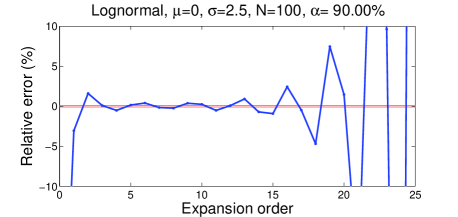
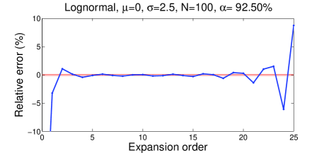
The convergence properties of the perturbative series are also of great importance. Even though a formal analysis of this question is beyond the scope of this work, we have carried out an empirical investigation of the accuracy of the approximation as a function of the order at which the perturbative expansion is truncated. The results reported are for sums of a fixed number of lognormal iidrv’s. Nonetheless, similar patterns are obtained for other distributions (e.g. Pareto) in other ranges of parameters and in sums of iidrv’s with random numbers of terms. In Figure 1, the relative error of the quantile estimations for a sum of $N=100$ lognormal iidrv’s is plotted as a function of the order of the perturbative expansion, for different quantile levels. From these results it is apparent that the series converges only asymptotically for $\alpha\rightarrow 1^{-}$. The asymptotic behavior of the series is analyzed in detail for the particular case of the Pareto distribution in section 5.3.3. For a fixed quantile level, the accuracy of the approximation initially improves as more terms are included in the expansion, but becomes worse beyond a certain order. Nonetheless, for a given order, there is a quantile level above which the series truncated to this order is a more accurate approximation than the series truncated to lower orders. As heavier tails imply stronger dominance of the maximum in the sum, the heavier the tails of the distribution, the more accurate of the approximation becomes. Hence, the order beyond which the approximation deteriorates is larger for distributions with heavier tails. Finally, the accuracy of the perturbative expansion becomes poorer for increasing $N$.

Figure 1: Relative error for Lognormal ($\sigma=2.5$) with frequency $N=100$, as a function of the coefficient order for $\alpha=90\%$ (upper plot), $\alpha=92.5\%$ (middle plot) and $\alpha=95\%$ (lower plot). The horizontal lines delimit the 95% confidence interval of the Monte Carlo simulation of the exact quantile.

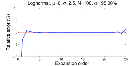In summary, in the cases analyzed, the accuracy of the approximation initially improves as more terms are included in the perturbative approximation. However, beyond a certain order, adding further terms in the expansion leads to an increase of the error. In the experiments carried out in the remainder of this section, the series is truncated at intermediate orders ($K=3$ or $K=5$), which, for the considered examples, provide very accurate approximations. The results of these experiments are presented in separate subsections, each of which corresponds to different types of distributions of the individual random variables in the sum.

5.1 Lévy distribution

In this section we evaluate the accuracy of the different approximations of high percentiles of the sum of iidrv’s that follow a Lévy distribution

$$f(x) =\sqrt{\frac{c}{2\pi}}\frac{1}{x^{3/2}}e^{-\frac{c}{2x}}$$ (69)

$$F(x) =\hbox{erfc}\left(\sqrt{\frac{c}{2x}}\right)\quad\text{for\ }x>0,$$

where $\hbox{erfc}(y)$ is the complementary error function. The mean of the Lévy distribution is infinite. The probability distribution, $F(x)$, is a function of regular variation $RV_{-a}$ and the density, $f(x)$, is $RV_{-(1+a)}$) with $a=1/2$. This a particularly useful case to analyze because the Lévy distribution belongs to the family of stable distributions [32]. Therefore, the sum of $N$ Lévy independent identically distributed (iid) random variables $Z_{N}=\sum_{i=1}^{N}L_{i}$, is also of the Lévy form

$$g(z) =\sqrt{\frac{c}{2\pi}}N\frac{1}{z^{3/2}}e^{-\frac{cN^{2}}{2z}}$$ (70)

$$G(z) =\hbox{erfc}\left(\sqrt{\frac{c}{2z}}N\right)=1-\hbox{erf}\left(\sqrt{\frac{c}{2z}}N\right)$$

Figure 2: Absolute value of the relative error of the different approximations to the $\alpha$-percentile of the sum of $N$ independent identically distributed Lévy random variables as a function of $\alpha$ for $N=100$ (upper plot) and $N=1000$ (lower plot).

Figure 3: Relative error of the different approximations to the percentile of the sum of iid Lévy random variables as a function of the number of terms in the sum for $\alpha=99\%$ (upper plot) and $\alpha=99.9\%$ (lower plot).

In the case of deterministic $N$, the $\alpha$-percentile is

$$Q=\frac{c}{2}N^{2}\left[\hbox{erf}^{-1}\left(1-\alpha\right)\right]^{-2}.$$ (71)

For Lévy random variables, $c_{a}=0$ in (64) because $a=1/2$. In consequence, the second order asymptotic approximation (64) coincides with the single-loss approximation

$$Q_{OW} =Q_{OW}^{*}=Q_{SL}=F^{-1}\left(1-\frac{1-\alpha}{N}\right)$$ (72)

$$=\frac{c}{2}\left[\hbox{erf}^{-1}\left(\frac{1-\alpha}{N}\right)\right]^{-2}.$$

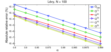
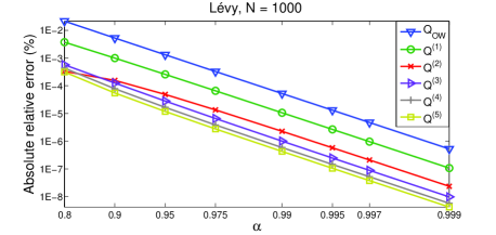
The accuracy of this approximation is compared to the perturbative series up to order $5$. Figure 2 displays in a logarithmic scale in both axes the absolute value of the relative error of the different approximations as a function of $\alpha$ for $N=100$ and $N=1000$. All approximations become more accurate for higher percentiles ($\alpha\rightarrow 1^{-}$). In this limit the relative error is proportional to $\left(1-\alpha\right)^{2}$ for all the approximations considered. Using the results of Appendix E the relative error of approximation (72) is

$$\frac{Q_{OW}-Q}{Q}\approx\frac{\pi}{6}\frac{N^{2}-1}{N^{2}}\left(1-\alpha\right)^{2}\quad\alpha\rightarrow 1^{-}.$$ (73)

Similarly, for the perturbative expansion truncated at different orders

$$\frac{Q^{(k)}-Q}{Q}\approx\gamma_{k}\left(1-\alpha\right)^{2}\quad\alpha\rightarrow 1^{-},\ k=1,2,\ldots,$$ (74)

with

$$\gamma_{1} = \frac{(2\pi-5)N^{2}-6(\pi-3)N+(4\pi-13)}{12N^{2}}$$

$$\gamma_{2} = \frac{(N-1)(N-2)}{6N^{2}}\left(\pi-3\right)$$

$$\gamma_{3} = \frac{(N-1)(N-2)}{6N^{2}}\left(\pi-\frac{16}{5}\right).$$ (75)

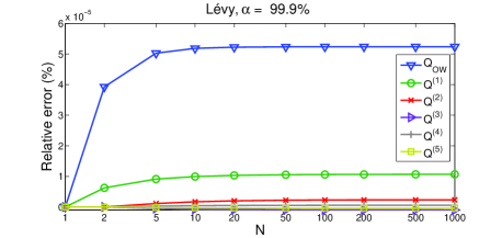
Up to the orders analyzed the perturbative series provides more accurate estimates than (72), improving with the number of terms included in this series. Nonetheless, the relative improvements become smaller for higher order terms. The dependence of the relative error with $N$, the number of terms in the sum, for $\alpha=99\%$ (upper plot) and $\alpha=99.9\%$ (lower plot) is shown in Figure 3. The relative error increases with $N$. Nonetheless, the deterioration is fairly slow. The error eventually approaches a constant, in agreement with the large $N$ behavior of (5.1). Also in these cases the perturbative series is more accurate that $Q_{OW}$.

5.2 Lognormal distribution

In this section we analyze the sum of iidrv’s that follow a lognormal distribution

$$f(x) =\frac{1}{x\sigma\sqrt{2\pi}}\exp\left(-\frac{(\log x)^{2}}{2\sigma^{2}}\right)$$ (76)

$$F(x) =\frac{1}{2}+\frac{1}{2}\hbox{erfc}\left(\frac{\log x}{\sigma\sqrt{2}}\right),\quad\text{for\ }x>0.$$

The lognormal is also subexponential. However, in contrast to the Lévy distribution, all its moments are finite. The perturbative series, which is of the same form as in the previous case, also provides very accurate approximations of high percentiles of the sum.

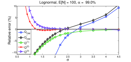
Figure 4 displays the relative error of the different approximations as a function of $\sigma$. Larger values of $\sigma$ correspond to heavier tails. In the simulations the number of terms in the sum (frequency) is random and follows a Poisson distribution whose mean is $\lambda=100$. In all cases, the relative error becomes smaller as $\sigma$ increases. This is consistent with the fact that this parameter determines the heaviness of the tail. For larger values of $\sigma$ (heavier tails) the relative importance of the maximum in the sum increases and the approximations, which are based on the dominance of the maximum in the sum, become more accurate.

Figure 4: Relative error for Lognormal /Poisson ($\lambda=100$) as a function of $\sigma$ for $\alpha=99\%$ (upper plot) and $\alpha=99.9\%$ (lower plot).

Figure 5: Relative error for Lognormal($\sigma=2$)/Poisson as a function of $\alpha$ for $\mathtt{E}[N]=100$ (upper plot) and as a function of $\mathtt{E}[N]$ for $\alpha=99.9\%$ (lower plot)

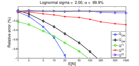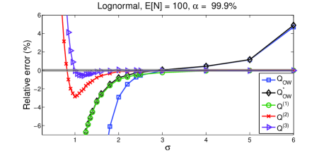
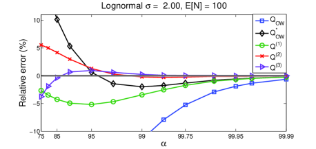
The second order asymptotic approximations $Q_{OW}^{*}$ and $Q_{OW}$ diverge as $\sigma$ becomes larger. This is not unexpected because the mean of the distribution increases as $e^{\sigma^{2}/2}$, while the percentile of the maximum (which dominates the sum) increases only as $e^{\sigma}$. The perturbative expansion introduced in this work, which involves only censored moments, avoids this problem and behaves properly. Figure 5 displays the dependence of the error of the different approximations as a function of the percentile level (upper plot) and of the average frequency (lower plot). As expected, all approximations perform better at higher percentiles and lower frequencies; that is, as the weight of the maximum in the sum becomes larger. Even for the relatively high average frequency $\lambda=1000$, the accuracy of the perturbative approximation $Q^{(3)}$ is remarkable.

5.3 Pareto distribution

In this section we analyze the sum of iidrv’s that follow a Pareto distribution

$$f(x)=\frac{a}{x^{1+a}},\quad F(x)=1-\frac{1}{x^{a}},\quad x>1,$$ (77)

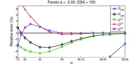
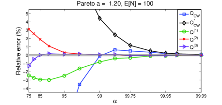
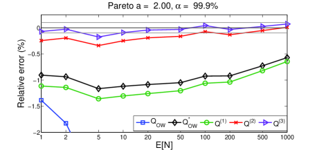
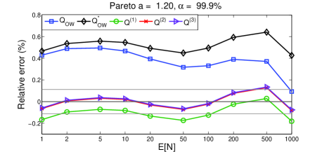
with $a>0$. Since the second order asymptotic approximations have a different form depending on whether the mean is defined or not, we consider two separate regimes: $a>1$, where the mean of the Pareto distribution is finite, and $a\leq 1$, where the mean diverges. It is worth noting that the perturbative expansion introduced in this work has the same expression in both regimes and is in fact continuous at $a=1$.

Figure 6: Relative error for Pareto / Poisson ($\lambda=100$) as a function of $a$ for $\alpha=99\%$ (upper plot) and $\alpha=99.9\%$ (lower plot). The values of $a$ are ordered so that the heaviness of the tails increases from left to right in the plots.

Figure 7: Relative error for Pareto / Poisson ( $\lambda=100$ ) as a function of $\alpha$ for different values of $a$: $a=2.00$ (upper plot) and $a=1.20$ (lower plot).

Figure 8: Relative error for Pareto/Poisson as a function of $\mathtt{E}[N]$ for $\alpha=99.9\%$ and different values of $a$: $a=2.00$ (upper plot) and $a=1.20$ (lower plot).

5.3.1 Pareto distribution with finite mean $(a>1)$:

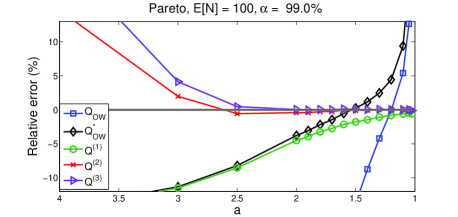
We now compare the accuracy of the different approximations for sums of random variables that follow a Pareto distribution with finite mean using Monte Carlo simulations. Figure 6 displays the relative error as a function of the Pareto index $a$. In the limit $a\rightarrow 1^{+}$ the second order asymptotic approximations $Q_{OW}$ and $Q_{OW}^{*}$ diverge. The origin of this divergence is the increase of correction term in (62,63), which involves the unconditional mean of the distribution. This mean which grows without bound as $a$ approaches $1$ from above. By contrast, the perturbative expansion, which is expressed in terms of censored moments, behaves well and actually becomes more accurate in this limit. Figure 7 presents the dependence of the relative error as a function of $\alpha$. The dependence on the average frequency $\lambda=\mathtt{E}[N]$ is shown in Figure 8. In all cases the conclusions reached through the analysis of these results are similar to the lognormal case.

5.3.2 Pareto distribution with infinite mean $(0<a\leq 1)$:

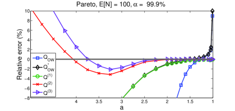
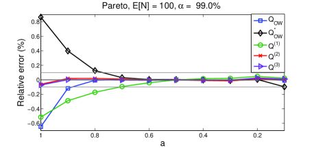
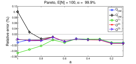
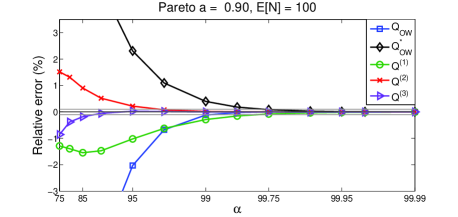
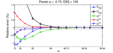
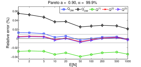
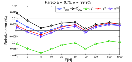
We now evaluate the accuracy of the different approximations for the percentiles of sums of random variables that follow a Pareto distribution with infinite mean. Figure 9 displays the relative error of the different approximations as a function of $a$, the tail parameter of the Pareto distribution. Figure 10 plots the relative error as a function of $\alpha$ for two different values of $a$. Finally, the change in relative error as the average frequency $\mathtt{E}[N]$ varies is presented in Figure 11. In this regime all approximations are fairly accurate. Between the second order asymptotic approximations, $Q_{OW}$ is more accurate than $Q_{OW}^{*}$.

For high percentiles, the best results corresponds to $Q^{(3)}$, the third order perturbative approximation. Beyond $\alpha=0.90$ the errors of this approximation are below the uncertainty of the Monte Carlo estimates. The improvements with respect to the standard approximations, $Q_{OW}$ or $Q_{OW}^{*}$, are especially significant for values of $a$ close to $1$.

Figure 9: Relative error for Pareto/Poisson ($\lambda=100$) as a function of $a$ for $\alpha=99\%$ (upper plot) and $\alpha=99.9\%$ (lower plot). The values of $a$ are ordered so that the heaviness of the tails increases from left to right in the plots.

Figure 10: Relative error for Poisson/Pareto as a function of $\alpha$ for $\lambda=100$ and different values of $a$.

Figure 11: Relative error for Poisson/Pareto as a function of $\mathtt{E}[N]$ for $\alpha=99.9\%$ and different values of $a$.

5.3.3 Effective expansion parameter

Equation (2) has been derived using a purely formal expansion parameter $\epsilon$, which is eventually set to $1$. In this section we take advantage of the simple form of the Pareto distribution to identify the actual perturbative parameter of the expansion for this type of random variables. To this end, we analyze the leading contributions in the individual terms in the expansion for $\alpha\rightarrow 1^{-}$. In terms of the parameter $\delta=(1-\alpha)$, the leading contributions for $\delta\rightarrow 0^{+}$ and for all non-integer $a\neq\frac{1}{2}$ are

$$\frac{Q_{1}}{N-1}\sim -\frac{a}{a-1}\left(\frac{\delta}{N}\right)^{1-1/a}+\ldots$$

$$+\frac{a}{a-1}\left(\frac{\delta}{N}\right)^{0/a}+\ldots$$

$$\frac{Q_{2}}{N-1}\sim -\frac{a(2a-1)}{a-2}\left(\frac{\delta}{N}\right)^{1-1/a}+\ldots$$

$$-\frac{a(a+1)}{(a-1)^{2}(a-2)}\left(\frac{\delta}{N}\right)^{1/a}+\ldots$$

$$\frac{Q_{3}}{N-1}\sim -\frac{2a(a-1)(2a-1)}{a-3}\left(\frac{\delta}{N}\right)^{1-1/a}+\ldots$$

$$+\frac{2a(a+1)^{2}(a+2)}{(a-1)^{3}(a-2)(a-3)}\left(\frac{\delta}{N}\right)^{2/a}+\ldots$$ (78)

The pattern that emerges is the following: up to order $Q_{k}$, with $k<a$, the terms $(\delta/N)^{(k-1)/a}$ dominate. Therefore, for $k<a$, $(\delta/N)^{1/a}$ can be interpreted as an expansion parameter. For $k>a$ the terms proportional to $(\delta/N)^{1-1/a}$ dominate. Since these terms are independent of $k$, there is no longer a recognizable expansion parameter. However, the prefactors, which depend on $a$, become smaller as the order of the perturbative term increases. For $k=a$ both types of terms contribute. It is interesting to note that the dominance shifts precisely at the order in which the moments cease to exist.

6 Conclusions

Starting from a perturbative expansion for the percentile of a sum of two random variables we derive a formal expansion for the percentile of sum of $N$ independent random variables. Assuming that, for sufficiently high percentiles, the maximum dominates the sum, the expansion is carried around the percentile of the maximum in the sum. This zeroth order term in the perturbative series is similar to the single-loss approximation [14], which can be derived from a first order asymptotic analysis of the tails of sums of subexponential random variables [38]. The first order perturbative correction is similar to the mean-corrected single-loss formula for distributions with finite mean [31], which can also be derived using higher order asymptotics. Higher order terms in the perturbative series are expressed in terms of right-truncated moments. These censored moments are always finite, regardless of whether the original uncensored distributions have finite or divergent moments. The perturbative series becomes more accurate for higher percentiles and heavier tails. From the empirical study carried out using either exact results or Monte Carlo simulation, one concludes that the perturbative approach is more accurate than previous approximate formulas proposed in the literature [25, 26, 30]. Furthermore, the accuracy of the approximation can be improved by including more terms in the perturbative series, up to a certain order. Beyond this order the approximation error generally increases. Another practical difficulty is the computational cost of the computations of higher order terms. Nonetheless, the third order approximation is sufficiently accurate for the percentiles ($99-99.9\%$), and the types of distributions that are used in practice in many fields of application, such as finance and insurance. As an extension of this research, the perturbative analysis is being applied to sums of random variables that are not identically distributed and may have dependencies. A more detailed analysis of the convergence of the perturbative series and the development of accurate approximations for lower percentiles are also the subject of current investigation.

Appendix A Complete Bell polynomials

The complete Bell polynomials (CBP) (named after Bell, [41]) arise in many contexts, such as the n-times differentiation of a function (Faà di Bruno formula) or to express the relationship between moments and cumulants in statistics.

Let $z(t)$ be an arbitrary function of $t$ whose $k$-th derivative $z^{(k)}(t)=\frac{d^{k}}{dt^{k}}z(t)$ the complete Bell polynomial of order $k$ is

$$B_{k}(z^{(1)}(t),\ldots,z^{(k)}(t))=e^{-z(t)}\frac{d^{k}}{dt^{k}}e^{z(t)}$$ (79)

From this definition, the CBP can be shown to satisfy

$$\exp{\left(\sum_{p=1}^{\infty}x_{p}\frac{t^{p}}{p!}\right)}=1+\sum_{q=1}^{\infty}B_{q}\left(x_{1},\ldots,x_{q}\right)\frac{t^{q}}{q!}.$$ (80)

This expression provides a relationship between the power series expansion of the moment generating function and the cumulant generating function. In partucular

$$\mu_{q}=B_{q}(\kappa_{1},\ldots,\kappa_{q}),$$ (81)

where $\mu_{q}$ are the moments of a random variable and $\kappa_{p}$ its cumulants.

In this paper we use a centered version of the CBP, which is defined by $C_{k}(x_{2},\ldots,x_{k})\equiv B_{k}(0,x_{2},\ldots,x_{k})$. In terms of $C_{k}(x_{2},\ldots,x_{k})$ the complete Bell polynomial of order $k$ is

$$B_{k}(x_{1},\ldots,x_{k})=\sum_{s=0}^{k}\binom{k}{s}x_{1}^{s}C_{k-s}(x_{2},\ldots,x_{k-s})$$ (82)

The CBP satisfy the following recursive formulae

$$k=0, \quad B_{0}=1\quad,\quad C_{0}=1$$ (83)

$$k=1, \quad B_{1}(x_{1})=x_{1}\quad,\quad C_{1}=0$$

$$k\geq 2, \quad B_{k}(x_{1},\ldots,x_{k})=$$

$$\quad x_{k}+\sum_{s=1}^{k-1}\binom{k-1}{s-1}x_{s}B_{k-s}(x_{1},\ldots,x_{k-s})$$

$$\quad C_{k}(x_{2},\ldots,x_{k})=$$

$$\quad x_{k}+\sum_{s=2}^{k-2}\binom{k-1}{s-1}x_{s}C_{k-s}(x_{2},\ldots,x_{k-s})$$

There exists an alternative representation for the CBP, which is related to the structure of the partitions of a set of size $n$

$$B_{k}(x_{1},\ldots,x_{k})=\sum_{\mathtt{A}\in\mathcal{P}(k)}\prod_{\mathtt{b}\in\mathtt{A}}x_{|\mathtt{b}|}$$ (84)

where $\mathcal{P}(k)$ is the set of all partitions of the set $\{1,\ldots,k\}$ (if $k=0$, $\mathcal{P}(k)$ contains one empty set) and $|\mathtt{b}|$ denotes the number of elements in set $\mathtt{b}$.

Appendix B Explicit formulas for particular frequency distributions

In this section we provide explicit formulas for the first terms in the perturbative series when the number of terms in the sum is distributed as a Poisson or as a negative binomial.

B.0.1 Poisson distribution

We consider the particular case where $N$, the number of terms in the sum (33) follows a Poisson distribution with parameter $\lambda=\mathtt{E}[N]$

$$p_{n}=\frac{1}{n!}\lambda^{n}e^{-\lambda}.$$ (85)

The moment generating function is

$$\mathcal{M}_{N}(s) =\exp{\left(\lambda(e^{s}-1)\right)}.$$ (86)

From this we derive

$$\lambda_{0}(x) =\exp{\left(\lambda(F(x)-1)\right)}\lambda f(x)$$ (87)

$$\lambda_{1}(x) =\lambda F(x)\lambda_{0}(x)$$

$$\lambda_{2}(x) =(1+\lambda F(x))\lambda_{1}(x).$$

The first three terms of the perturbative expansion are

$$Q_{0} =F^{-1}\left(\frac{\log{\alpha}}{\lambda}+1\right)$$

$$Q_{1} =\left(\lambda+\log{\alpha}\right)\mathtt{E}\left[L|L<Q_{0}\right]$$

$$Q_{2} =-\frac{1}{\lambda_{0}(Q_{0})}\partial_{x}\left(\lambda_{1}(x)(\kappa_{2}(x)+\kappa_{1}(x)^{2})\right)_{x=Q_{0}}$$

$$=-\left(\lambda f(Q_{0})+\frac{f^{\prime}(Q_{0})}{f(Q_{0})}\right)(\log{\alpha}+\lambda)\mathtt{E}[L^{2}|L<Q_{0}]$$

$$\hskip 9.95863pt-\lambda f(Q_{0})Q_{0}^{2},$$

where, in the last step, we have used the identity

$$\partial_{x}\mu_{p}(x)=\frac{f(x)}{F(x)}\left(x^{p}-\mu_{p}(x)\right).$$ (88)

for the censored moments $\mu_{p}(x)\equiv\mathtt{E}[L^{p}|L<x]$.

B.0.2 The negative binomial distribution

The probability mass function of the negative binomial distribution with parameters $(p,r)$ is

$$p_{n}=\binom{n+r-1}{n}p^{r}(1-p)^{n}.$$ (89)

Setting $q\equiv 1-p$ The moment generating function is

$$\mathcal{M}_{N}(s)=p^{r}\left[1-qe^{s}\right]^{-r}.$$ (90)

In terms of $\xi(x)=1-qF(x)$ we have

$$\lambda_{0}(x) =p^{r}{\xi(x)}^{-r-1}qrf(x)$$ (91)

$$\lambda_{1}(x) ={\xi(x)}^{-1}q(1+r)F(x)\lambda_{0}(x)$$

$$\lambda_{2}(x) ={\xi(x)}^{-1}\left[1+q(1+r)F(x)\right]\lambda_{1}(x)$$

The first three terms in the perturbative expansion are

$$Q_{0} =F^{-1}\left(\frac{1-p{\alpha}^{-1/r}}{q}\right)$$ (92)

$$Q_{1} =(1+r)\left(\frac{\alpha^{1/r}}{p}-1\right)\mathtt{E}\left[L|L<Q_{0}\right]$$

$$Q_{2} =-\frac{r+1}{h^{3}}\Bigg{[}$$

$$\mathtt{E}\left[L^{2}|L<Q_{0}\right]h(1-h)\left(q(r+2)f(Q_{0})+h\frac{f^{\prime}(Q_{0})}{f(Q_{0})}\right)$$

$$+\mathtt{E}\left[L|L<Q_{0}\right]^{2}(1-h)^{2}\left(q(r+3)f(Q_{0})+h\frac{f^{\prime}(Q_{0})}{f(Q_{0})}\right)$$

$$+\mathtt{E}\left[L|L<Q_{0}\right]2Q_{0}qh(1-h)f(Q_{0})+{Q_{0}}^{2}qh^{2}f(Q_{0})\Bigg{]}$$

where $q\equiv 1-p$ and $h\equiv p\alpha^{-1/r}$.

Appendix C Recursive formulas for the perturbative series

The objective of this section is to derive recursive expressions for the terms in the perturbative expansion of high quantiles of $Z=X+\epsilon Y$. These expressions are better suited for the numerical computation of the series than the expressions derived in section 2.
The starting point is (8). By defining the function

$$\phi(s,x)\equiv f_{X}(x)\mathcal{M}_{Y|X}(s|x),$$ (93)

where

$$\mathcal{M}_{Y|X}(s|x)=\int_{-\infty}^{\infty}\,dy\,e^{sy}f_{Y|X}(y|x)$$ (94)

is the moment generation function of $Y$ conditional on $X$, and the operator

$$\Omega_{\epsilon}\equiv\left(e^{\left(\delta Q-\epsilon\partial_{s}\right)\partial_{x}}-1\right)\partial_{x}^{-1},$$ (95)

(8) can be written as

$$\left.\Omega_{\epsilon}\phi(s,x)\right|_{s=0,x=Q_{0}}=0.$$ (96)

By defining the operators $\left\{\Omega^{(n)}\equiv\frac{\partial^{n}\Omega_{\epsilon}}{\partial\epsilon^{n}}|_{\epsilon=0},\ n\geq 0\right\}$, the terms of the perturbative expansion can be obtained by solving the equations

$$\left.\Omega^{(n)}\phi(s,x)\right|_{s=0,x=Q_{0}}=0\,,\,\,\,\text{for all }\,\,\,n\geq 0.$$ (97)

The sequence of operators $\Omega^{(n)}$ has the recurrence relation

$$\Omega^{(0)} = 0$$

$$\Omega^{(1)} = \widetilde{\partial}_{s}$$

$$\Omega^{(k)} = Q_{k}+\Omega^{(k-1)}\widetilde{\partial}_{s}\partial_{x}+\displaystyle{\sum_{i=1}^{k-2}}\binom{k-1}{i}Q_{k-i}\Omega^{(i)}\partial_{x}$$ (98)

for $k\geq 2$ and with $\widetilde{\partial}_{s}\equiv Q_{1}-\partial_{s}$. Expressing each operator $\Omega^{(n)}$ in the form

$$\Omega^{(k)}=\sum_{i=0}^{n}\sum_{j=0}^{n}\omega_{i,j}^{(k)}\widetilde{\partial}_{s}^{i}\partial_{x}^{j}$$ (99)

(C) can be expressed as recursion relations for the coefficients

$$\omega^{(k)}_{0,0} =Q_{k}$$

$$\omega^{(k)}_{i,0} =0$$

$$\omega^{(k)}_{0,j} =\displaystyle{\sum_{l=\max(1,j-1)}^{k-2}}\binom{k-1}{l}Q_{k-l}\omega_{0,j-1}^{(l)}$$

$$\omega^{(k)}_{i,j} =\displaystyle{\sum_{l=\max(1,i,j-1)}^{k-2}}\binom{k-1}{l}Q_{k-l}\omega_{i,j-1}^{(l)}+\omega_{i-1,j-1}^{(k-1)},$$ (100)

for $i,j\geq 1$. Finally, the terms in the perturbative series can be derived from (97) as

$$Q_{n}=-\frac{1}{\phi^{(0,0)}}\sum_{i=0}^{n}\sum_{j=1}^{n}\omega_{i,j}^{(n)}\phi^{(i,j)}$$ (101)

where

$$\phi^{(i,j)}\equiv\left.\widetilde{\partial}_{s}^{i}\partial_{x}^{j}\phi(s,x)\right|_{s=0,x=Q_{0}}.$$ (102)

The remainder of this appendix is devoted to the derivation of explicit recursive formulas for the quantities $\phi^{(i,j)}$ of the perturbative expansion for sums of $N$ independent random variables, $Z_{N}=\sum_{n=1}^{N}L_{n}$. These independent rv’s are identically distributed according to $F(l)$ (density $f(l)$).

C.1 Deterministic $N$

Consider the case of sums of $N$ iidrv’s, with $N$ fixed. In this case, the expansion around the maximum of the terms in the sum is characterized by

$$f_{X}(x) =NF(x)^{N-1}f(x)$$

$$\mathcal{M}_{Y|X}(s|x) =\mathcal{M}_{L}(s|x)^{N-1}.$$ (103)

Therefore

$$\phi(s,x)=Nf(x)F(x)^{N-1}\mathcal{M}_{L}(s|x)^{N-1}.$$ (104)

To make the notation more compact, the following definitions are used in the derivation

$$\mathcal{M}_{Y|X}^{(i,j)} \equiv\left.\partial_{s}^{i}\partial_{x}^{j}\mathcal{M}_{L}^{N-1}(s|x)\right|_{s=0,x=Q_{0}}$$

$$k_{i}^{(j)} \equiv\left.\partial_{x}^{j}\kappa_{i}(x)\right|_{x=Q_{0}}=\left.\partial_{s}^{i}\partial_{x}^{j}\log\mathcal{M}_{L}(s|x)\right|_{s=0,x=Q_{0}}$$

$${m}^{(j)}_{i} \equiv\left.\partial_{x}^{j}\mu_{i}(x)\right|_{x=Q_{0}}=\left.\partial_{s}^{i}\partial_{x}^{j}\mathcal{M}_{L}(s|x)\right|_{s=0,x=Q_{0}}$$

$$\tilde{F}^{(j)} \equiv\left.\partial_{x}^{j}\log F(x)\right|_{x=Q_{0}}$$

$$\tilde{f}^{(j)} \equiv\left.\partial_{x}^{j}\log f(x)\right|_{x=Q_{0}}\,,$$ (105)

where

$$\mathcal{M}_{L}(s|x)=\int_{0}^{x}dl\,e^{sl}\,\frac{f(l)}{F(x)}$$ (106)

is the generating function of the censored moments of the individual terms in the sum with censoring threshold $x$.

Using these expressions and definitions, the coefficients in (101) are

$$\phi^{(i,j)}=\sum_{l=0}^{i}\sum_{k=0}^{j}(-1)^{i-l}\binom{j}{k}\binom{i}{l}Q_{1}^{l}\mathcal{M}_{Y|X}^{(i-l,j-k)}\left.\partial_{x}^{k}f_{X}(x)\right|_{x=Q_{0}}.$$ (107)

The derivatives of the conditional moment generating function $\mathcal{M}_{Y|X}(s|x)$ evaluated at $s=0$ and $x=Q_{0}$ can be computed using the recursion

$$\mathcal{M}_{Y|X}^{(0,j)} =\delta_{0,j}$$

$$\mathcal{M}_{Y|X}^{(i,j)} =(N-1)\displaystyle{\sum_{l=0}^{i-1}\sum_{k=0}^{j}}\binom{i-1}{l}\binom{j}{k}\mathcal{M}_{Y|X}^{(l,k)}k_{i-l}^{(j-k)}$$ (108)

for $j\geq 0$, $i\geq 1$ and with $\delta_{i,j}$ the Kronecker delta. To evaluate this expression one needs the derivatives of the censored cumulants evaluated at $Q_{0}$. These can be computed using the recursion

$$k_{0}^{(j)} =0$$

$$k_{i}^{(j)} =m_{i}^{(j)}-\displaystyle{\sum_{l=1}^{i-1}\sum_{k=0}^{j}}\binom{i-1}{l}\binom{j}{k}m_{l}^{(k)}k_{i-l}^{(j-k)}$$ (109)

for $j\geq 0$, $i\geq 1$. Finally, the derivatives of the censored moments evaluated at $Q_{0}$ are given by the recursion

$$m_{i}^{(j)}=\displaystyle{\sum_{k=0}^{j-1}\binom{j-1}{k}}\tilde{F}^{(1+k)}\left(\left.\partial_{x}^{j-1-k}x^{i}\right|_{x=Q_{0}}-m_{i}^{(j-1-k)}\right),$$ (110)

for $j\geq 1$. Besides $m_{i}^{(0)}$, the censored moments with threshold $x=Q_{0}$, the remaining terms in the calculation, namely, the derivatives of logarithm of the severity $\tilde{F}^{(j)}$ and of the density of the maximum $\partial_{x}^{k}f_{X}(x)=\partial_{x}^{k}\left(Nf(x)F(x)^{N-1}\right)$ can be readily computed from the derivatives of the severity CDF, also via recursion. For instance

$$\tilde{F}^{(j)}=\frac{\left[\partial_{x}^{j}F(x)-\displaystyle{\sum_{k=1}^{j-1}\binom{j-1}{k}\partial_{x}^{k}F(x)\tilde{F}^{(j-k)}}\right]_{x=Q_{0}}}{F(Q_{0})}.$$ (111)

C.2 Random $N$

In this case

$$\mathcal{M}_{Y|X}(s|x) =\mathbb{E}\left[e^{SY}\big{|}X=x\right]$$

$$=\sum_{n=0}^{\infty}\mathcal{M}_{Y|X,N}(s|x,n)\frac{f_{X_{n}}(x)p_{n}}{f_{X}(x)}$$

$$=\sum_{n=0}^{\infty}\mathcal{M}_{L}(s|x)^{n-1}\frac{f_{X_{n}}(x)p_{n}}{f_{X}(x)}$$ (112)

with $p_{n}\equiv\mathbb{P}[N=n]$. In terms of these quantities

$$\phi(s,x)=\mathbb{E}\left[f_{X_{N}}(x)\mathcal{M}_{L}(s|x)^{N-1}\right].$$ (113)

The coefficients in (101) are then given by

$$\phi^{(i,j)} =\sum_{l=0}^{i}\binom{i}{l}Q_{1}^{l}(-1)^{i-l}\partial_{s}^{i-l}\partial_{x}^{j}\mathbb{E}\Big{[}f_{X_{N}}(x)\mathcal{M}_{L}^{N-1}(s,x)\Big{]}_{s=0}^{x=Q_{0}}$$

$$=\sum_{l=0}^{i}\binom{i}{l}Q_{1}^{l}(-1)^{i-l}\xi^{(i-l,j)}_{0},$$ (114)

where

$$\xi^{(i,j)}_{a}=\partial_{s}^{i}\partial_{x}^{j}\mathbb{E}\Big{[}(N-1)^{a}f_{X_{N}}(x)\mathcal{M}_{L}^{N-1}(s,x)\Big{]}_{s=0}^{x=Q_{0}}.$$ (115)

These quantities have the recursion

$$\xi^{(0,j)}_{a} =\partial_{x}^{j}\mathbb{E}\Big{[}(N-1)^{a}f_{X_{N}}(x)\Big{]}_{x=Q_{0}}=\left.\partial_{x}^{j}\lambda_{a}(x)\right|_{x=Q_{0}}$$

$$\xi^{(i,j)}_{a} =\displaystyle{\sum_{l=0}^{i-1}\sum_{k=0}^{j}}\binom{i-1}{l}\binom{j}{k}\xi^{(l,k)}_{a+1}k_{i-l}^{(j-k)}i\geq 1,\,j\geq 0$$ (116)

where the coefficients $\lambda_{a}(x)$ have been defined in (47). Their values at $x=Q_{0}$ can be computed using equation (49) in terms of the derivatives of the moment generating function. To obtain the derivatives $\lambda_{a}^{(k)}\equiv\left.\partial_{x}^{k}\lambda_{a}(x)\right|_{x=Q_{0}}$ in the previous equation, the following recursion can be used

$$\lambda_{a}^{(k)}=\sum_{l=0}^{k-1}\binom{k-1}{l}\Big{(}\tilde{f}^{(l+1)}\lambda_{a}^{(k-l-1)}+\tilde{F}^{(l+1)}\lambda_{a+1}^{(k-l-1)}\Big{)}.$$ (117)

The remaining elements in the calculation (moments, censored cumulants and their derivatives etc.) are computed as in the case with deterministic $N$.

Appendix D Derivation of higher order asymptotic approximations

In this section we present the derivations of the single-loss approximation and higher order corrections that have been given in the literature. [22, 23, 25, 26, 27, 28, 29, 30]

D.1 Second order approximation by Omey and Willekens [22, 23]

It is possible to derive corrections to the single-loss approximation by using the second order behavior of the tail probability of subordinate distributions [22, 23]. These references are also the basis for the analysis presented in [25, 26].

For the case in which the mean is finite, the second order approximation for the tail distribution of the sum is [23]

$$1-G(x)\sim\mathtt{E}\left[N\right]\left(1-F(x)\right)+\mathtt{E}\left[N(N-1)\right]\mu_{L}f(x)\quad\quad x\rightarrow\infty.$$ (118)

From this, it is possible to derive a nonlinear equation for a second order approximation of $Q\equiv G^{-1}(\alpha)$, the percentile of the sum at the probability level $\alpha$

$$Q\approx F^{-1}\left[1-\frac{1-\alpha}{\mathtt{E}\left[N\right]}+\left(\frac{\mathtt{E}\left[N^{2}\right]}{\mathtt{E}\left[N\right]}-1\right)\mu_{L}f\left(Q\right)\right].$$ (119)

This nonlinear equation can be solved numerically.

A closed-form expression that is similar to the correction by the mean proposed in [31] is obtained using an approximate solution of

$$1-\alpha\sim\mathtt{E}\left[N\right]\left(1-F(Q)\right)+\epsilon\mathtt{E}\left[N(N-1)\right]\mu_{L}f(Q)$$ (120)

where the parameter $\epsilon=1$ has been introduced to order the terms in a perturbative expansion of the solution

$$Q={Q^{\prime}}_{0}+\epsilon{Q^{\prime}}_{1}+\ldots$$ (121)

Expanding (120) up to first order in $\epsilon$ we obtain

$$1-\alpha = \mathtt{E}\left[N\right]\left(1-F({Q^{\prime}}_{0}+\epsilon{Q^{\prime}}_{1}+\ldots)\right)$$

$$+\epsilon\mathtt{E}\left[N(N-1)\right]\mu_{L}f({Q^{\prime}}_{0}+\epsilon{Q^{\prime}}_{1}+\ldots)$$

$$1-\alpha = \mathtt{E}\left[N\right]\left(1-F({Q^{\prime}}_{0})\right)$$

$$-\epsilon\Big{(}\mathtt{E}\left[N\right]f({Q^{\prime}}_{0}){Q^{\prime}}_{1}-\mathtt{E}\left[N(N-1)\right]\mu_{L}f({Q^{\prime}}_{0})\Big{)}$$

$$+{\cal O}(\epsilon^{2})$$

Identifying terms of the same order,

$$1-\alpha =\mathtt{E}\left[N\right]\left(1-F({Q^{\prime}}_{0})\right)\quad\Longrightarrow$$

$$\quad\quad{Q^{\prime}}_{0}=F^{-1}\left(1-\frac{1-\alpha}{\mathtt{E}\left[N\right]}\right),$$ (122)

$$0 =\left(\mathtt{E}\left[N\right]{Q^{\prime}}_{1}-\mathtt{E}\left[N(N-1)\right]\mu_{L}\right)f({Q^{\prime}}_{0})\quad\Longrightarrow$$

$$\quad\quad{Q^{\prime}}_{1}=\left(\frac{\mathtt{E}\left[N^{2}\right]}{\mathtt{E}\left[N\right]}-1\right)\mu_{L},$$ (123)

which provides a good approximation to the solution provided that $f({Q^{\prime}}_{0})>0$ and ${Q^{\prime}}_{1}\ll{Q^{\prime}}_{0}$. Therefore, the approximate solution of (120) with $\epsilon=1$ is

$$Q\approx F^{-1}\left(1-\frac{1-\alpha}{\mathtt{E}\left[N\right]}\right)+\left(\mathtt{E}\left[N\right]+(D-1)\right)\mu_{L},$$ (124)

where $D=\mathtt{Var}\left[N\right]/\mathtt{E}\left[N\right]$ is the index of dispersion ($D=1$ for the Poisson distribution and $D>1$ for the negative binomial distribution). The first term in (124) is the single-loss formula. The second term is a correction that involves the mean.

Similar approximate formulas can be given for the case of distributions $F(L)$ with infinite mean and whose corresponding density is regularly varying $f(L)\in RV_{-(1+a)}$ using the results of [22]

$$1-G(x) \sim\mathtt{E}\left[N\right]\left(1-F(x)\right)+c_{a}\mathtt{E}\left[N(N-1)\right]\mu_{F}(x)f(x)$$

$$\text{for}\quad x\rightarrow\infty,$$ (125)

where

$$\mu_{F}(x)\equiv\int_{0}^{x}ds(1-F(s))=(1-F(x))x+F(x)\mathtt{E}\left[L|\leq x\right],$$ (126)

and

$$c_{a}=\left\{\begin{array}[]{ll}1&a=1\\ (1-1/a){\frac{\left[\Gamma(1-a)\right]^{2}}{2\Gamma(1-2a)}}&a<1\end{array}\right..$$ (127)

In this case a second order approximation of $Q\equiv G^{-1}(\alpha)$ can be obtained from

$$Q\approx F^{-1}\left(1-\frac{1-\alpha}{\mathtt{E}\left[N\right]}+c_{a}\left(\frac{\mathtt{E}\left[N^{2}\right]}{\mathtt{E}\left[N\right]}-1\right)\mu_{F}(Q)f(Q)\right).$$ (128)

Again, this nonlinear equation can be solved numerically using, for example, an iterative scheme. Alternatively, an approximate closed-form expression can be obtained by means of a perturbative scheme analogous to the finite mean case

$$Q \approx {Q^{\prime}}_{0}+c_{a}\left(\mathtt{E}\left[N\right]+(D-1)\right)\mu_{F}({Q^{\prime}}_{0}),$$ (129)

$${Q^{\prime}}_{0} = F^{-1}\left(1-\frac{1-\alpha}{\mathtt{E}\left[N\right]}\right)$$ (130)

$$\mu_{F}({Q^{\prime}}_{0}) = \int_{0}^{{Q^{\prime}}_{0}}\left(1-F(s)\right)ds$$

$$= \frac{1-\alpha}{\mathtt{E}\left[N\right]}{Q^{\prime}}_{0}+\left(1-\frac{1-\alpha}{\mathtt{E}\left[N\right]}\right)\mathtt{E}\left[L|L\leq{Q^{\prime}}_{0}\right],$$

D.2 Asymptotic expansion by Barbe and McCormick [27, 28, 29]

This section uses the approximations for the distribution of sums of independent random variables with heavy tails derived in [27, 28, 29]. For simplicity, we assume that the number of terms in the sum are sampled from a Poisson distribution. Assuming that the first $m$ moments of the variables in the sum are finite

$$1-G(x) =\lambda\exp\left\{\lambda\sum_{i=1}^{m}\frac{(-1)^{i}}{i!}\mu_{L}^{[i]}\partial_{x}^{i}\right\}\left[1-F(x)\right]$$

$$+\mathcal{O}\left(h^{m}(x)\left[1-F(x)\right]\right),$$ (132)

where $h(x)=f(x)/(1-F(x))$ and $\mu_{L}^{[i]}\equiv E[L^{i}]=\int_{0}^{\infty}dx\,f(x)x^{i}$ is the $i$th moment of $L$. For $m=0$, the single-loss approximation is recovered. The first order approximation ($m=1$) is

$$1-G(x)\approx\lambda e^{-\lambda\mu_{L}\partial_{x}}\left[1-F(x)\right].$$ (133)

In [28, 29] the authors proceed by preforming a Taylor expansion of the right-hand side of (133). Here, we derive an exact formula by realizing that the Taylor expansion can be resummed. This resummation results in a translation of the argument of $F$

$$1-G(x)\approx\lambda\left[1-F(x-\lambda\mu_{L})\right].$$ (134)

Therefore, the first order approximation to the $\alpha$ percentile of $G$ yields the correction by the mean

$$Q\approx F^{-1}\left(1-\frac{1-\alpha}{\lambda}\right)+\lambda\mu_{L},$$ (135)

also in this derivation. The second order approximation for $G$ can also be expressed in terms of an integral over a diffusion kernel

$$1-G(x) \approx\lambda\Bigg{[}1-\int_{0}^{\infty}\,dz\,\frac{1}{\sqrt{2\pi\lambda\mu_{L}^{[2]}}}\times$$

$$\quad\quad\quad\exp\left\{-\frac{\left(z-x+\lambda\mu_{L}\right)^{2}}{2\lambda\mu_{L}^{[2]}}\right\}F(z)\Bigg{]}.$$ (136)

The corresponding second order approximation ($m=2$) for $Q$, the $\alpha$ percentile of $G$ is the solution of the nonlinear equation

$$1-\alpha =\lambda\Bigg{[}1-\int_{0}^{\infty}\,dz\,\frac{1}{\sqrt{2\pi\lambda\mu_{L}^{[2]}}}$$

$$\quad\quad\quad\exp\left\{-\frac{\left(z-Q+\lambda\mu_{L}\right)^{2}}{2\lambda\mu_{L}^{[2]}}\right\}F(z)\Bigg{]}.$$ (137)

D.3 Asymptotics with a shifted argument

The results of this section are based on the expansion for $G$ derived in [30] using only evaluations of $F$ at different arguments

$$1-G(x)\approx\mathtt{E}\left[N\right]\left(\xi_{1}F(x-k_{1})+\ldots+\xi_{m}F(x-k_{m})\right)$$ (138)

for some constants $\xi_{1},\ldots,\xi_{m}$, $k_{1},\ldots,k_{m}$. Assuming that the first $m$ moments of $F$ are finite, these constants are the solution of the system of equations

$$\sum_{j=1}^{m}\xi_{j} = 1$$

$$\sum_{j=1}^{m}\left(c_{i}-\mathtt{E}\left[N\right]k_{j}^{i}\right)\xi_{j} = 1;i=1,\ldots,m,$$ (139)

where $c_{i}=\mathtt{E}\left[N\left(X_{1}+\ldots+X_{N}\right)^{i}\right];\ \text{for}\ \geq 0$. There is some freedom in the choice $k_{1},\ldots,k_{m}$. In [30] the authors propose to determine the values of these parameters by enforcing the constraints

$$\sum_{j=1}^{m}\left(c_{m+i}-\mathtt{E}\left[N\right]k_{j}^{m+i}\right)\xi_{j}=0,\quad\text{for}\quad i=1,\ldots,m-1.$$ (140)

Therefore, the approximation of order $m$ is obtained by solving the set of nonlinear equations

$$\sum_{j=1}^{m}\xi_{j}k_{j}^{i}=\tilde{c}_{i},\quad\text{for}\quad i=0,\ldots,2m-1.$$ (141)

where $\tilde{c}_{i}=c_{i}/\mathtt{E}\left[N\right]\ \text{for}\ i\geq 0$.

For $m=1$

$$\xi_{1}=1,\quad\quad k_{1}=\tilde{c}_{1}=\frac{c_{1}}{\mathtt{E}\left[N\right]}=\frac{\mathtt{E}\left[N(N-1)\right]}{\mathtt{E}\left[N\right]}\mu_{L},$$ (142)

which yields the first order approximation

$$1-G(x)\approx\mathtt{E}\left[N\right]F(x-\frac{\mathtt{E}\left[N(N-1)\right]}{\mathtt{E}\left[N\right]}\mu_{L}).$$ (143)

The $\alpha$ percentile of $G$ in this approximation is the single-loss formula corrected by the mean (124).

Appendix E Approximations to high percentiles of sums of Lévy iidrv’s

The exact $\alpha$ quantile for the sum of $N$ Levy iidrv’s with parameters $(\mu=0,c)$ is

$$Q=\frac{c}{2}N^{2}\left[\hbox{erf}^{-1}(\delta)\right]^{-2},$$ (144)

where $\delta=1-\alpha$. High percentiles can be approximated as

$$Q\approx\frac{2c}{\pi}N^{2}\Bigg{[}\frac{1}{\delta^{2}}-\frac{\pi}{6}-\frac{\pi^{2}}{120}\delta^{2}+\mathcal{O}(\delta^{4})\Bigg{]},\quad\delta\rightarrow 0^{+}.$$ (145)

For the Lévy distribution the approximation to the quantiles (64) is

$$Q_{OW}=\frac{c}{2}\left[\hbox{erf}^{-1}\left(\frac{\delta}{N}\right)\right]^{-2}.$$ (146)

For high percentiles, this approximation is of the form

$$Q_{OW}\approx\frac{2c}{\pi}\Bigg{[}\frac{N^{2}}{\delta^{2}}-\frac{\pi}{6}+\mathcal{O}\left(\left(\frac{\delta}{N}\right)^{2}\right)\Bigg{]},\quad\delta\rightarrow 0^{+}.$$ (147)

Similarly, it is possible derive the high-percentile approximations of the perturbative expansion coefficients

$$Q_{0}\approx \frac{2N^{2}c}{\pi}\Bigg{[}\frac{1}{\delta^{2}} -\frac{N-1}{N}\frac{1}{\delta} +\frac{(N-1)(N-5)-2\pi}{12N^{2}} +\mathcal{O}(\delta)\Bigg{]}$$ (148)

$$Q_{1}\approx \frac{2N^{2}c}{\pi}\Bigg{[} \frac{N-1}{N}\frac{1}{\delta} -\frac{(N-1)(N+\pi-3)}{2N^{2}} +\mathcal{O}(\delta)\Bigg{]}$$

$$Q_{2}\approx \frac{2N^{2}c}{\pi}\Bigg{[} -\frac{(N-1)(N+1)}{6N^{2}} +\mathcal{O}(\delta)\Bigg{]}$$

$$Q_{3}\approx \frac{2N^{2}c}{\pi}\Bigg{[} -\frac{(N-1)(N-2)}{5N^{2}} +\mathcal{O}(\delta)\Bigg{]}.$$

References

- [1] Saralees Nadarajah. A review of results on sums of random variables. Acta Applicandae Mathematicae, 103:131–140, 2008.
- [2] J.W. Cohen. On the tail of the stationary waiting-time distribution and limit theorem for M/G/1 queue. Annales de l’Institut Henri Poincaré, 8:255–263, 1972.
- [3] Gilles Faÿ, Bárbara González-Arévalo, Thomas Mikosch, and Gennady Samorodnitsky. Modeling teletraffic arrivals by a poisson cluster process. Queueing Systems, 54:121–140, 2006.
- [4] P. Embrechts, C. Klüppelberg, and T. Mikosch. Modelling extremal events for insurance and finance. Applications of mathematics. Springer, 1997.
- [5] A.J. McNeil, R. Frey, and P. Embrechts. Quantitative risk management: concepts, techniques and tools. Princeton series in finance. Princeton University Press, 2005.
- [6] Antoine Frachot, Pierre Georges, and Thierry Roncalli. Loss distribution approach for operational risk. Working paper, Groupe de Recherche Opérationnelle, Crédit Lyonnais, France (2001), 2001.
- [7] Paul Embrechts, Hansjörg Furrer, and Roger Kaufmann. Quantifying regulatory capital for operational risk. Derivatives Use, Trading & Regulation, 9(3):217–233, 2003.
- [8] H.H. Panjer. Operational Risk: Modeling Analytics. Wiley, New York, 2006.
- [9] Santiago Carrillo-Menéndez and Alberto Suárez. Robust quantification of the exposure to operational risk: Bringing economic sense to economic capital. Computers & OR, pages 792–804, 2012.
- [10] S. A. Klugman, H. H. Panjer, and G. E. Willmot. Loss Models: from Data to Decisions, 2nd edn. Wiley, 2004.
- [11] B. Dupire. Monte Carlo: methodologies and applications for pricing and risk management. Risk Books, 1998.
- [12] Søren Asmussen, Klemens Bingswanger, and Bjarne Højgaard. Rare events simulation for heavy-tailed distributions. Bernoulli, 6:303–322, 2000.
- [13] Søren Asmussen and Dirk P. Kroese. Improved algorithms for rare event simulation with heavy tails. Advances in Applied Probability, 38(2):545–558, 2006.
- [14] K. Böcker and C. Klüppelberg. Operational var: a closed-form approximation. Risk, December:90–93, 2005.
- [15] Charles M. Goldie and Claudia Klüppelberg. Subexponential distributions. In Robert J. Adler, R. Feldman, and M. S. Taqqu, editors, A Practical Guide to Heavy Tails: Statistical Techniques and Applications, pages 435–459. Birkhäuser, Boston, MA, 1998.
- [16] S. Foss, D. Korshunov, and S. Zachary. An Introduction to Heavy-Tailed and Subexponential Distributions. Springer Series in Operations Research and Financial Engineering. Springer, 2011.
- [17] R.D. Reiss and M. Thomas. Statistical analysis of extreme values: with applications to insurance, finance, hydrology and other fields. Birkhäuser, 2007.
- [18] S. Asmussen. Applied probability and queues. Applications of mathematics. Springer, 2003.
- [19] Zoi Tsourti and John Panaretos. Extreme value analysis of teletraffic data. Computational Statistics & Data Analysis, 45:85–103, 2004.
- [20] Mark E. Crovella, Murad S. Taqqu, and Azer Bestavros. Heavy-tailed probability distributions in the World Wide Web, pages 3–25. Birkhauser Boston Inc., Cambridge, MA, USA, 1998.
- [21] S.I. Resnick. Heavy-tail phenomena: probabilistic and statistical modeling. Number v. 10 in Springer series in operations research. Springer, 2007.
- [22] E. Omey and E. Willekens. Second-order behaviour of the tail of a subordinated probability distribution. Stochastic Processes and their Applications, 21:339 – 353, 1986.
- [23] E. Omey and E. Willekens. Second-order behaviour of distributions subordinate to a distribution with finite mean. Communications in Statistics. Stochastic Models, 3(3):311 – 342, 1987.
- [24] Rudolf Grubel. On subordinated distributions and generalized renewal measures. Annals of Probability, 15(1):394–415, 1987.
- [25] Anupam Sahay, Zailong Wan, and Brian Keller. Operational risk capital: asymptotics in the case of heavy-tailed severity. The journal of operational risk, 2(2):61–72, 2007.
- [26] M. Degen. The calculation of minimum regulatory capital using single-loss approximations. Journal of Operational Risk, 5(4):3–17, 2010.
- [27] Philippe Barbe and William P. McCormick. Asymptotic expansions of convolutions of regularly varying distributions. Journal of the Australian Mathematical Society, 78(3):339–371, 2005.
- [28] Ph. Barbe, W. P. McCormick, and C. Zhang. Asymptotic expansions for distributions of compound sums of random variables with rapidly varying subexponential distribution. Journal of Applied Probability, 44(3):670–684, 2007.
- [29] P. Barbe and W.P. McCormick. Asymptotic expansions for infinite weighted convolutions of heavy tail distributions and applications. Memoirs of the American Mathematical Society. American Mathematical Society, 2009.
- [30] Hansjörg Albrecher, Christian Hipp, and Dominik Kortschak. Higher-order expansions for compound distributions and ruin probabilities with subexponential claims. Scandinavian Actuarial Journal, 2010(2):105–135, 2010.
- [31] K. Böcker and J. Sprittulla. Operational var: meaningful means. Risk, December:96–98, 2006.
- [32] J. P. Nolan. Stable Distributions - Models for Heavy Tailed Data. Birkhauser, Boston, 2012. In progress, Chapter 1 online at academic2.american.edu/jpnolan.
- [33] Saralees Nadarajah and M. Masoom Ali. The distribution of sums, products and ratios for lawrance and lewis’s bivariate exponential random variables. Computational Statistics & Data Analysis, 50(12):3449 – 3463, 2006.
- [34] C. Gourieroux, J.P. Laurent, and O. Scaillet. Sensitivity analysis of values at risk. Journal of Empirical Finance, 7:225–245, 2000.
- [35] R. Martin and T. Wilde. Unsystematic credit risk. Risk, 15(11):123–128, 2002.
- [36] M. Blum. On the sums of independently distributed Pareto variates. SIAM Journal on Applied Mathematics, 19(1):191–198, July 1970.
- [37] V. P. Chistyakov. A theorem on sums of independent positive random variables and its applications to branching random processes. Theory of Probability and its Applications, 9(4):640–648, 1964.
- [38] P. Embrechts and N. Veraverbeke. Estimates for the probability of ruin with special emphasis on the possibility of large claims. Insurance: Mathematics and Economics, 1(1):55 – 72, 1982.
- [39] N. H. Bingham, C. M. Goldie, and J. L. Teugels. Regular Variation. Cambridge University Press, 1987.
- [40] Basel Committee on Banking Supervision. International Convergence of Capital Measurement and Capital Standards. A Revised Framework. June 2006.
- [41] E.T. Bell. Exponential polynomials. Annals of Mathematics, 35:258–277, 1934.