Methanol and excited OH masers towards W51: I - Main and South

Abstract

MERLIN phase-referenced polarimetric observations towards the W51 complex were carried out in March 2006 in the Class II methanol maser transition at 6.668 GHz and three of the four excited OH maser hyperfine transitions at 6 GHz. Methanol maser emission is found towards both W51 Main and South. We did not detect any emission in the excited OH maser lines at 6.030 and 6.049 GHz down to a 3$\sigma$ limit of $\sim$20 mJy beam^-1. Excited OH maser emission at 6.035-GHz is only found towards W51 Main. This emission is highly circularly polarised (typically $\geq 45$ % and up to 87%). Seven Zeeman pairs were identified in this transition, one of which contains detectable linear polarisation. The magnetic field strength derived from these Zeeman pairs ranges from $+1.6$ to $+6.8$ mG, consistent with the previously published magnetic field strengths inferred from the OH ground-state lines. The bulk of the methanol maser emission is associated with W51 Main, sampling a total area of $\sim 3\arcsec\times 2.2$″ (i.e., $\sim 16200\times 11900$ AU), while only two maser components, separated by $\sim$2.5″, are found in the W51 South region. The astrometric distributions of both 6.668-GHz methanol and 6.035-GHz excited-OH maser emission in the W51 Main/South region are presented here. The methanol masers in W51 Main show a clear coherent velocity and spatial structure with the bulk of the maser components distributed into 2 regions showing a similar conical opening angle with of a central velocity of $\sim$+55.5 km s^-1 and an expansion velocity of $\leq$5 km s^-1. The mass contained in this structure is estimated to be at least 22 M_⊙. The location of maser emission in the two afore-mentioned lines is compared with that of previously published OH ground-state emission. Association with the UCHII regions in the W51 Main/South complex and relationship of the masers to infall or outflow in the region are discussed.

1 Introduction

W51, originally detected by Westerhout (1958), is one of the most massive Giant Molecular Clouds (GMCs) in the Galaxy (Mufson & Liszt 1979). This $1.6\times 10^{6}$ M_⊙ GMC (Carpenter & Sanders 1998) is a very rich high-mass star-forming region (SFR) environment, located in the Sagittarius spiral arm, which contains two giant HII regions labelled W51A and W51B which are themselves resolved into smaller components (Mehringer 1994). Within W51A, the most luminous site labelled W51e, where W51 Main/South is found, is one of the brightest regions. Trigonometric parallax measurements of the 22 GHz H₂O maser source in W51 Main/South from Sato et al. (2010) give a distance of $5.4\pm 0.3$ kpc for the complex. W51 Main/South has been studied at a wide range of wavelengths both in continuum and molecular (thermal and maser) transitions. It is known to host many ultra-compact (UC) HII regions thought to contain massive young stellar objects at various stages of evolution: the UCHII regions are labelled W51e1, e2, e3 and e4 (Gaume, Johnston & Wilson 1993). Of these, W51e2 was found to be composed of four more compact continuum sources labelled W51e2-W, e2-E, e2-NW and e2-N (Shi, Zhao & Han 2010a), and the UCHII region labelled W51e8 (Zhang & Ho 1997). Zhang, Ho, & Ohashi (1998) found evidence of gravitational infall towards W51e2 and W51e8. Kalenskii & Johansson (2010) performed a survey at 3 mm towards W51e1/e2 covering the frequency range 84-115 GHz that detected 105 molecules and their isotopic species. Maser emission from H₂O, ground-state OH, NH₃ and methanol has also been found (Genzel et al. 1978 & 1981; Menten, Melnick & Phillips 1990a; Menten et al. 1990b; Imai et al. 2002; Fish & Reid 2007; Zhang & Ho 1997; Phillips & van Langevelde 2005). Excited OH maser emission at 6.035 GHz towards W51 has also been detected and observed on several occasions (Rickard, Zuckerman & Palmer 1975; Caswell & Vaile 1995; Desmurs & Baudry 1998) but its actual provenance in the SFR complex has not been ascertained yet.

We have performed MERLIN astrometric observations of excited-OH maser emission at 6.035, 6.030 and 6.049 GHz and Class II methanol maser emission at 6.668 GHz towards W51 to investigate the relationship between the maser emission and the compact continuum sources in this SFR complex. Here we present the results regarding W51 Main/South. The other regions of the W51 complex will be presented in a subsequent paper. We compare the distribution of the detected 6.035-GHz excited-OH and 6.668-GHz methanol maser emission to that of the ground-state OH in the same region. Additional information regarding the magnetic field strength and structure of the region is also discussed. The details of the observations and the data reduction are presented in section 2. The results are presented in section 3. The OH maser modelling carried out for the present study is presented in section 4. A discussion of the results is given in section 5. A summary and conclusions are presented in section 6.

2 Observations and data reduction

Observations were performed using the six telescopes of MERLIN available at 5 cm at that time (namely Defford, Cambridge, Knockin, Darnhall, MK2 & Tabley) in full polarimetric mode. The two excited OH maser main lines at a rest frequency of 6.030747 and 6.035092 GHz were observed on 2006 March 21 while the satellite OH maser line at a rest frequency of 6.049084 GHz and the methanol maser transition at a rest frequency of 6.668518 GHz were observed on 2006 March 20, 25 and 30. For all the transitions, a spectral bandwidth of 0.5 MHz divided into 512 channels was used, giving a velocity coverage of 22.745 and 24.855 km s^-1 and a channel spacing of 0.044 and 0.049 km s^-1 for the 6.668 GHz methanol and 6.035 GHz excited OH maser datasets, respectively. The central velocity was taken to be $v_{\rm LSR}=+55.50$ km s^-1 for all observations. All the velocities given in this paper are relative to the local standard of rest (LSR). The observations of the target at all transitions were interspersed with short periods on the same phase reference calibrator, 1920+154. 3C84 was used as the bandpass calibrator and for the polarisation leakage (d-term) corrections. 3C286 was used to retrieve the absolute polarisation position angles and to provide the flux density reference. The data reduction followed the procedure explained in section 2 of Etoka, Cohen & Gray (2005).

The initial data editing, the gain-elevation correction and a first-order amplitude calibration were applied using the d-program, a MERLIN-specific package available at Jodrell (Diamond et al. 2003). Further refined data editing, the remaining instrumental and atmospheric effect calibrations, bandpass and second order amplitude calibrations and phase referencing were performed within the aips package (Diamond et al. 2003, Appendix F).

The final phase calibration on the source was performed using the brightest channel in the RHC polarisation of the 6.035 GHz excited OH dataset with transfer of solutions onto the LHC polarisation. For the 6.668 GHz methanol dataset the second strongest channel was used as it led to a better phase calibration. With an intensity ratio of roughly 10 between the reference channel adopted and the brightest channel we estimate that the intensity inferred for the strongest component is underestimated by $\sim$10%.

The accuracy in absolute position for the masers is limited by four factors: (1) the position accuracy of the phase calibrator, (2) the accuracy of the telescope positions, (3) the relative position error proportional to the beamsize and inversely proportional to the signal-to-noise ratio, and finally (4) the atmospheric variability. The first two factors are frequency independent and were estimated to be $\sim$5 mas (given by the MERLIN calibrator catalogue) and 10 mas (Diamond et al. 2003) respectively. The third factor is very small in comparison to the other sources of error (2-3 mas in the worst case). The fourth error is estimated from the quality of the phase of the calibrator and its separation from the source. Given the angular separation of 1.2°, we estimate that this final error is less than 8 mas. All these errors add quadratically to give 14 mas as the total systematic error in the absolute positions measured in this paper.

All the offset positions given from here onwards are with respect to the reference position, taken to be that of Comp 24 of the methanol 6.668 GHz dataset (marked with an asterisk in Table 1), namely, RA_J2000=$19^{\rm h}23^{\rm m}43\aas@@fstack{s}948$ Dec_J2000=14°30′34$\aas@@fstack{\prime\prime}$38 $\pm 14$ milliarcsec. Given that the 6-GHz excited OH and 6.668-GHz methanol datasets were obtained with the same instrument a few days appart, an extra quadratic atmospheric variability term needs to be taken into consideration for the calculation of the alignment uncertainty. Consequently, the accuracy of the alignment of the two maser types is $16$ mas.

The source was imaged with the task imagr using a pixel separation of 5 mas. The restoring beamwidth at 6.668 GHz was 78 $\times$ 48 mas² with a position angle (P.A.) of 22$\degr$. At 6.035 GHz the restoring beamwidth was 64 $\times$ 45 mas² with a P.A. of 23$\degr$. Typically, the rms noise level ($\sigma$), obtained from the image of a channel free of emission, was about 7 mJy beam^-1 for the 6.668-GHz methanol dataset, increasing to 150 mJy beam^-1 in the channel with the strongest emission. For the 6.035 GHz excited OH dataset the $\sigma$ was typically 14 mJy increasing to 18 mJy in the channel with the strongest emission.

The datacubes were inspected and the maser emission features were fitted with two-dimensional Gaussians using the task sad with a flux threshold of 3$\sigma$. Maser spots were grouped as ‘components’ for further analysis if they showed emission in at least three consecutive frequency channels with relative positional offsets of less than 25 mas.

Polarisation information was retrieved for the 6-GHz excited OH maser emission. At the position of each maser component found in the Stokes $I$ data cube, the flux in Stokes $Q$, $U$ and $V$ were measured. The linear polarised intensity $P=\sqrt{Q^{2}+U^{2}}$ and polarisation angle $\chi=0.5\times$arctan($U/Q$) were then calculated for each maser component. $P$ is considered significant only if it is greater than 3$\sigma$.

3 Results

3.1 Methanol maser emission at 6.668 GHz

Table 1 presents in decreasing velocity order the components detected in the 6.668-GHz methanol maser transition over the W51 Main/South region. Column 1 gives the component number, Column 2 gives its intensity-weighted velocity, Column 3 gives its specific intensity and Columns 4 and 5 give its RA and Dec offset from the reference position.

Table 1: 6.668-GHz methanol maser components

Comp	Vel	I	$\Delta\alpha$a	$\Delta\delta$a
Nb	(km s-1)	(Jy b-1)	(mas)	(mas)
1	64.046	0.285	-1558.7	-9590.8
2	60.841	0.182	862.4	177.7
3	60.434	2.853	206.8	177.8
4	60.151	8.622	11.9	43.8
5	60.142	0.449	866.0	501.5
6	60.019	24.462	5.8	57.8
7	59.290	216.410	3.5	66.6
8	58.821	26.625	67.0	-79.0
9	58.807	2.654	16.9	171.7
10	58.796	0.986	132.4	-158.1
11	58.738	1.347	72.4	249.1
12	58.736	1.337	274.3	88.5
13	58.712	2.936	9.8	-18.6
14	58.684	2.002	3.3	144.3
15	58.672	1.814	37.4	35.7
16	58.555	0.809	69.3	66.8
17	58.515	1.458	925.3	162.9
18	58.413	0.550	279.0	-91.2
19	58.393	1.377	157.5	52.2
20	58.390	0.656	-29.1	126.1
21	58.317	3.177	681.0	414.2
22	58.238	4.221	274.5	100.3
23	58.231	0.959	273.2	110.2
∗24	58.007	28.387	0.0	0.0
25	57.429	0.298	942.3	153.9
26	57.326	0.900	-356.9	2273.1
27	56.805	0.117	1012.8	1077.0
28	56.786	0.092	976.9	1093.6
29	55.331	0.360	-895.5	-7103.6
30	54.954	0.230	-484.5	-148.0
31	53.008	0.237	-737.1	378.4
32	52.888	0.115	-298.0	-289.1
33	52.811	0.198	-1024.9	22.2
34	52.778	0.549	717.3	1354.4
35	52.593	0.331	-1003.3	42.7
36	52.476	0.718	-1025.8	31.1
37	52.371	1.611	-366.9	-434.4
38	52.248	0.629	-1003.4	244.4
39	52.175	0.146	-947.4	37.6
40	52.157	0.141	-181.4	-381.5
41	51.947	4.288	-193.6	-239.8
42	51.880	0.994	-387.7	-473.5
43	51.860	0.728	-981.0	248.3
44	51.631	1.077	621.9	1030.8
45	51.525	2.174	-392.0	-467.9
46	51.500	0.308	-787.0	-291.9
47	51.053	0.599	-199.8	-239.0
48	51.018	0.150	-900.6	223.1
49	50.904	0.247	-422.1	-480.0
50	49.934	0.198	623.3	969.2

$\bf a:$ $\Delta\alpha$ and $\Delta\delta$ are relative to the reference position taken to be that of Comp 24 (marked with an asterisk):

RA_J2000=$19^{\rm h}23^{\rm m}43\aas@@fstack{s}948$ Dec_J2000=14°30′34$\aas@@fstack{\prime\prime}$38.

Figures 1 and 2 present the spectra constructed from the final images for the regions, seemingly distinct in the plane of the sky, where 6.668 GHz methanol maser emission has been detected towards W51 Main and W51 South respectively. Unlike W3(OH) where a large-scale methanol maser filament has been found (Harvey-Smith & Cohen 2006) such an extended emission is not detected. Comparison of the spectral profile displayed in the main panel of Figures 1 with that obtained with the Australia Telescope Compact Array (ATCA) in May 2007 (Avison, PhD 2010), with an angular resolution of $\sim 40\arcsec$, shows a good agreement regarding the main spectral group of components observed and their relative intensity ratio, indicating that there is no substantial resolved emission Towards W51 Main, the overall area from which 6.668-GHz methanol maser is emitted covers $\sim$3″ $\times$ 2.2″ (i.e., $\sim 16200\times 11900$ AU), and can be divided roughly into four areas.

In W51 Main there seem to be 4 distinct regions of emission on the plane of the sky. The bulk of the emission arises from the multi-component peak in the velocity range [+57.0,+61] km s^-1 and comes from a region in W51 Main covering the area $\Delta\alpha$=[+500,-100] mas $\Delta\delta$=[-200,+300] mas (hereafter, the “central region”; Fig. 1c). The spectrum of the region located north-east of the central region and covering the area $\Delta\alpha$=[+1000,+500] mas $\Delta\delta$=[+100,+1400] mas (Fig. 1b) shows the largest spread in velocity, with a total velocity range of $\sim 8$ km s^-1. It is made of two main groups of components centred at $\sim+52.0$ km s^-1 and $\sim+58.2$ km s^-1. The latter group peak velocity is encompassed by the velocity range covered by the bluest group of components of the central region. The spectrum of the south-west region covering the area $\Delta\alpha$=[-100,-1100] mas $\Delta\delta$=[-500,+400] mas (Fig. 1e) encompasses a similar velocity range as that of the north-east blue peak. The spectrum from the faint group of components emanating from the northern region centered around $\Delta\alpha=-360$ mas $\Delta\delta=+2270$ mas (Fig. 1d) covers the bluer edge of the prominent multi-component peak.

Towards W51 South, only two localised areas are found to be producing 6.668-GHz methanol maser emission.

Figure 1: Spectra constructed from the final images for the various regions where 6.668-GHz methanol maser emission has been detected towards W51 Main. a) Spectrum for the entire region covering an area of $\sim$3″ $\times$ 2.2″. b) Spectrum for the north-east region covering the area $\Delta\alpha$=[+1000,+500] mas $\Delta\delta$=[+100,+1400] mas. c) Spectrum for the central region covering the area $\Delta\alpha$=[+500,-100] mas $\Delta\delta$=[-200,+300] mas. d) Spectrum for the northern region centered around $\Delta\alpha=-360$ mas $\Delta\delta=+2270$ mas. e) Spectrum for the south-west region covering the area $\Delta\alpha$=[-100,-1100] mas $\Delta\delta$=[-500,+400] mas. Note that the channels corresponding to the strongest peak covering the velocity range $\sim$[+59.0,+60.0] and $\sim$[+57.7,+60.5] km s^-1 have been set to zero for the spectra in $\bf b$ and $\bf d$ respectively due to the high level of noise in the corresponding images.

Figure 2: Spectra constructed from the final images for the two regions where 6.668-GHz methanol maser emission has been detected towards W51 South, covering in both cases an area of $\sim 250\times 250$ mas². a) Spectrum for the northern part. Note that the channels corresponding to the strongest peak covering the velocity range $\sim$[+58,+60.5] km s^-1 have been set to zero due to the high level of noise in the corresponding images. b) Spectrum for the southern part.

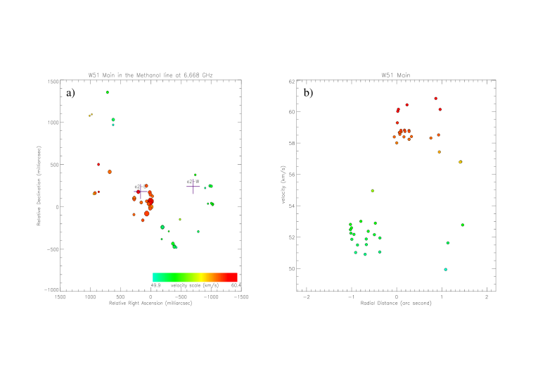
Figure 3: a) Maser components in the methanol 6.668-GHz line towards W51 Main, excluding the northern component, Comp 26, at the RA and Dec offsets $\Delta\alpha\sim-357$ mas and $\Delta\delta\sim+2273$ mas. The size of the symbols is proportional to the log of the intensity. The velocity colour-code is restricted to the W51 Main methanol maser emission velocity range. The crosses indicate the positions of the compact continuum sources in the region (Shi et al. 2010a). b) The velocity distribution of the maser spot versus radial distance. The central position is taken to be [0,+80 mas] inferred from the convergent point of the SW blue-shifted maser components.

Following the criteria given in section 2, 50 maser components were identified towards the W51 Main/South complex, only 2 of which are associated with W51 South. Figure 3a presents the maser component distribution in the methanol 6.668-GHz transition in W51 Main found around W51e2-E and W51e2-W. The velocity spread is 10.5 km s^-1 with a mean velocity at +55.5 km s^-1. The masers are not uniformly distributed but seem to be part of 3 main regions, two of which are seemingly distributed into ellipsoidal structures reminscent of what is observed in various SFR complexes by Bartkiewicz et al. (2009). The overall maser emission is roughly oriented along a P.A. $\simeq 70^{\degr}$ (east of north). The extent of the two largest ellipsoidal structures is similar: $\sim$1.2″ (i.e., $\sim$6500 AU) while that located at the centre is much smaller: $\leq$0.5″ (i.e., $\leq$2700 AU). Figure 3b presents the velocity distribution of the maser components versus the radial distance from a central position of [0,+80] mas which has been inferred from the converging points of the SW blue-shifted maser components. This position is within 15 mas of the strongest methanol maser spot (Comp 7 centered at $+59.3$ km s^-1 cf. Table 1), and in good agreement with the location of W51e2-E given the beam size of the SMA at 0.85 mm, 0$\aas@@fstack{\prime\prime}$3 $\times$ 0$\aas@@fstack{\prime\prime}$2. There is a clear position-velocity relation for the bulk of the maser components found to be distributed mainly into 2 regions showing a similar conical opening angle indicative of a central velocity of $\sim$+55.5 km s^-1 and an expansion velocity of $\leq$5 km s^-1.

It has to be noted that the systemic velocity for W51e2 estimated from the different hot molecular lines varies significantly, from $\sim+54$ to $\sim+59$ km s^-1 (e.g., Shi et al. 2010a; Sollins, Zhang & Ho 2004; Remijan et al. 2004; Zhang et al. 1998; Rudolph et al. 1990). The $\sim$+55.5 km s^-1 convergent central velocity inferred from Fig. 3b is in close agreement with the central velocity of the HCN(4-3) absorption line observed towards W51e2-E by Shi, Zhao & Han (2010b, their Fig 4b) and interpreted as being redshifted absorption of HCN against the compact continuum core.

The five components forming the northern part of the north-east ellipsoidal structure (covering the area $\Delta\alpha$=[+1000,+500] mas $\Delta\delta$=[+900,+1400] mas in the north-east region observed in Fig. 3a and found at the radial distance [+1.0″,+1.6″] in Fig. 3b) do not follow the velocity-position relation. As noted previously, the spectrum corresponding to the north-east ellipsoidal structure is the most extended one with a total velocity extent of $\sim$8 km s^-1 (cf. Fig 1b). These two facts seem to indicate that these masers, though appearing to probe a distinct ellipsoidal structure in the plane of the sky, actually trace different physical components in the W51 Main region. Moreover, the velocity distribution versus the radial distance (Fig. 3b) indicates that the southern redshifted part of this plane-of-the-sky structure (covering the area $\Delta\alpha$=[+1000,+500] mas $\Delta\delta$=[+100,+500] mas) is dynamically associated with the “central region”.

One maser component (Comp 26 in Table 1), centered at a velocity of $+57.3$ km s^-1, is found $\geq$2″ north of the bulk of the maser components in W51 Main, seemingly associated with either W51e2-N or W51e2-NW (0.5 and 0.65″ away from these cores respectively).

The two maser components detected in W51 South (Comp 1 and Comp 29 in Table 1) are centered at $\sim+64.0$ km s^-1 and $\sim+55.3$ km s^-1 respectively (cf. Fig 4 and Fig 2). The northern component, Comp 29, is closer to W51e8 ($\sim$0.5″) than it is to W51e1 ($\sim$1.1″) and is consequently more likely to be associated with W51e8, though the systemic velocity of this core has been estimated to be $\sim+59$ km s^-1 by Zhang et al. (1998). The southern component, Comp 1, is clearly associated with W51e3.

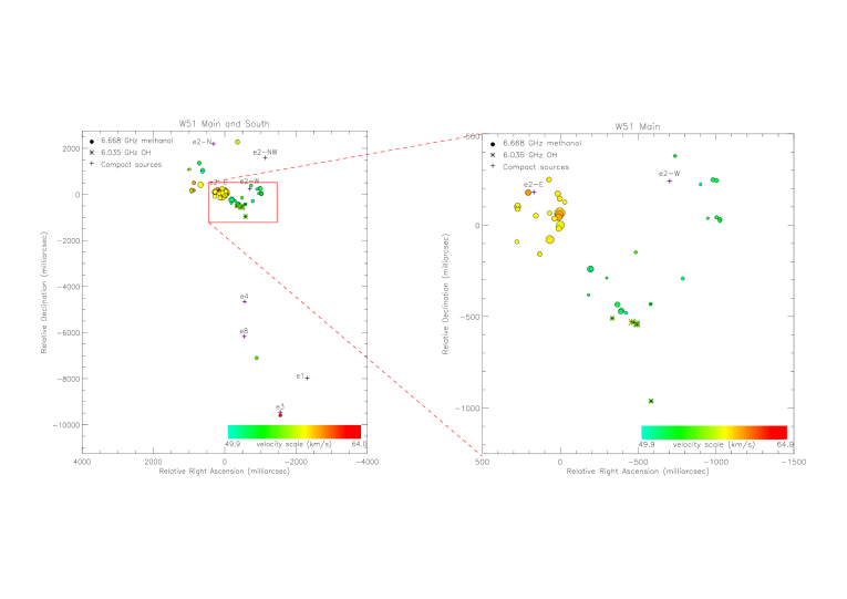
Figure 4: Left panel: Maser components in the methanol 6.668-GHz and the excited OH 6.035-GHz transitions for the overall W51 Main/South region. Right panel: Magnification of part of W51 Main. The velocity colour-code covers the W51 Main and South methanol maser emission velocity range. The size of the symbols is proportional to the log of the intensity. The crosses indicate the positions of the compact continuum sources in the region (Gaume et al. 1993, Zhang & Ho 1997, Shi, Zhao & Han 2010a).

3.2 Excited OH emission

The theoretical models by Gray, Field & Doel (1992) and Pavlakis & Kylafis (2000) show that the SFR regions are conducive to inversion of the 5-cm main lines (overlapping the range of conditions leading to the inversion of the ground-state main lines) and weak inversion of the satellite transition at 6.049 GHz, but unfavourable for 6.017 GHz inversion.

Observational studies show the presence of 6.035-GHz and to a lesser extent 6.031-GHz maser emission towards a wide range of high-mass SFR sites known to exhibit ground-state 1.665 GHz maser emission (e.g., Caswell 2003; Desmurs & Baudry 1998; Baudry et al. 1997; Caswell & Vaile 1995). Maser emission from these excited OH maser transitions is often present in regions similar to those that emit in the Class II methanol maser at 6.668 GHz (e.g., Green et al. 2007; Etoka et al. 2005). This is corroborated by the models by Cragg, Sobolev & Godfrey (2002) which show that very similar high-density, low-temperature conditions with a substantial radiation field at a higher temperature are needed for the inversion of these maser transitions.

We observed the three 6-GHz hyperfine transitions for which inversion in SFR regions can potentially occur. We did not detect any excited OH maser lines at 6.031 or 6.049 GHz towards the entire W51 complex down to a 3$\sigma$ limit of $\sim$20 mJy beam^-1.

3.2.1 6.035 GHz

Excited OH emission at 6.035 GHz towards the W51 complex was first detected by Rickard et al. (1975) and then reobserved on several occasions (Caswell & Vaile 1995; Desmurs & Baudry 1998). Two main spectral features are visible in the spectra of Rickard et al. (1975, their Fig. 4) covering a velocity range of $+52.8$ to $+56$ km s^-1 with the strongest emission at $\sim+53$ km s^-1. The spectra obtained by Caswell & Vaile (1995) clearly show five spectral features ranging from $+52.8$ to $+64$ km s^-1 with the strongest spectral feature at $\sim+55$ km s^-1. Figure 5 presents the 6.035-GHz excited OH spectra in the RHC (solid line) and LHC (dashed line) polarisations towards W51 Main from the present work. Two spectral features at $\sim+53$ and $\sim+57.5$ km s^-1 are clearly visible, with the stronger spectral feature at $\sim+57.5$ km s^-1 reaching a peak flux density of 6 Jy. Comparing the spectral profile observed in the 1970’s (Rickard et al.), 1990’s (Caswell & Vaile) and in the 2000’s (present work) it is clear that the emission is highly variable and is likely the explanation of the non-detection of the 2 faint spectral features at $\sim+59$ and $\sim+64$ km s^-1 detected by Caswell & Vaile (1995).

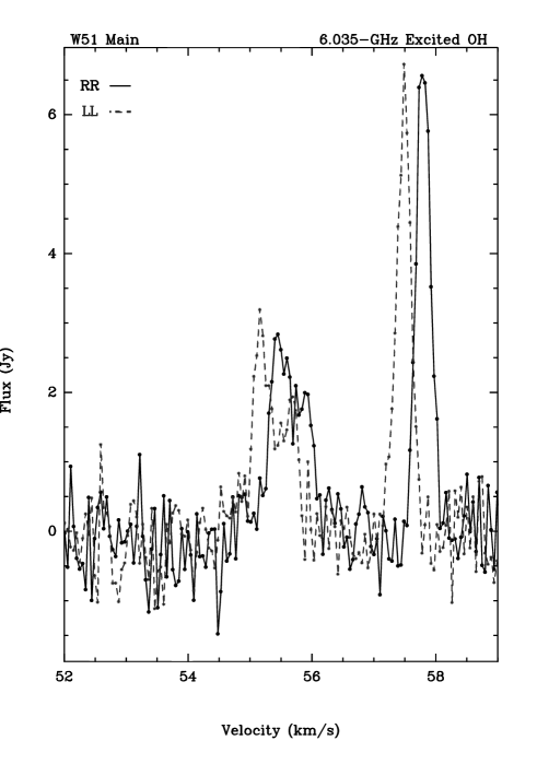
Figure 5: Spectra in the RHC (solid line) and LHC (dashed line) polarisations constructed from the final images over the entire area where 6.035-GHz excited OH emission is found towards W51 Main.

Table 2: 6.035-GHz RHC and LHC maser components

Comp	Vel	Flux	$\Delta\alpha$a	$\Delta\delta$a	Zb
	(km s-1)	(Jy b-1)	(mas)	(mas)
6.035 GHz	RHC
∗1RR	57.802	3.443	-460.2	-529.5	z1
2RR	56.833	0.296	-471.9	-530.3	z2
3RR	55.895	0.476	-334.3	-508.9	z3
4RR	55.747	1.473	-491.8	-542.5	z4
5RR	55.383	1.455	-489.2	-536.8	z5
6RR	54.954	0.581	-583.9	-962.2	z6
7RR	52.915	0.198	-585.2	-440.5	z7(⋄)
6.035 GHz	LHC
1LL	57.488	2.899	-460.2	-529.5	z1
2LL	56.451	0.255	-472.7	-532.6	z2
3LL	55.722	0.417	-332.6	-509.6	z3
4LL	55.656	0.895	-494.9	-546.1	z4
5LL	55.209	1.469	-490.9	-539.5	z5
6LL	54.725	0.463	-582.2	-962.9	z6
7LL	52.590	0.165	-575.1	-421.7	z7(⋄)

^∗: reference component

a: the $\Delta\alpha$ and $\Delta\delta$ are relative to the methanol reference maser spot position RA_J2000=$19^{\rm h}23^{\rm m}43\aas@@fstack{s}948$ Dec_J2000=14°30′34$\aas@@fstack{\prime\prime}$38

b: Zeeman pair labelling

$\diamond$: Comp 7_LL is quite faint and failed to pass the 3 consecutive channel criterion (it only passed the 2 consecutive channel criterion) but the Zeeman pattern is clearly visible in the spectra (Fig. 6).

Following the selection criteria given in section 2, seven maser components were identified in the RHC polarisation and six in the LHC. All of the 6 LHC components detected are associated with a RHC component in six Zeeman pairs at 6.035 GHz. These are presented in Table 2.

The average Zeeman flux ratio Flux_LL/Flux_RR is 0.83, ranging from 0.61 to 1.01. The seventh unpaired RHC component is the faintest component detected (less than 200 mJy). Taking into account the average flux ratio, the likelihood that this RHC component is also paired with a faint LHC counterpart that did not meet the 3 consecutive channel criterion was high. And, indeed, the LHC component met the 3$\sigma$ threshold only over 2 consecutive channels, but is clearly visible in the Stokes $V$ spectrum with a peak intensity of 165 mJy (Fig 6). Consequently, 100% of the emission detected in the excited OH line at 6.035 GHz is part of a Zeeman pairing.

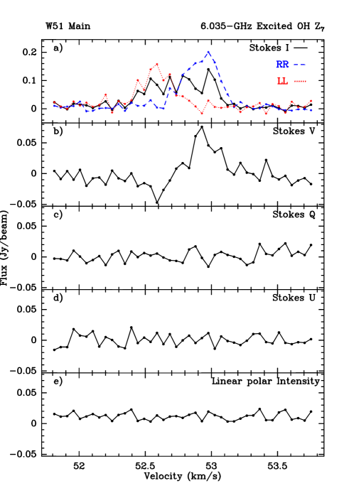
Figure 6: Spectra of the Zeeman pair z₇ (6.035-GHz excited OH line). a) Stokes $I$, RHC and LHC spectra. b) Stokes $V$. c) Stokes $Q$. d) Stokes $U$. e) linear polarisation intensity $P$.

Table 3 presents, in decreasing velocity order, the characteristics of the Zeeman pairs identified, as follows: Column 1 gives the Zeeman pair label, Column 2 gives the demagnetized velocity (that is the best estimate of the actual velocity of the component), Columns 3 and 4 give the RA and Dec offset from the reference position used in the present work respectively, Columns 5 to 8 give the Stokes $I$, $Q$, $U$ and $V$ intensity respectively, Column 9 gives the linear polarisation intensity $P$, Columns 10 to 12 give the circular, linear and total percentage of polarisation ($m_{\rm c}$, $m_{\rm l}$ and $m_{\rm t}$) respectively. In case of an elliptically polarised component (i.e., $m_{l}\geq 10$%) Column 13 gives its associated polarisation angle $\chi$, Column 14 gives the velocity split ($v_{\rm split}$=$v_{\rm(RHC)}$ - $v_{\rm(LHC)}$) and finally the corresponding magnetic field strength B is given in Column 15.

Table 3: 6.035-GHz Zeeman pair characteristics

Za	Velb	$\Delta\alpha$c	$\Delta\delta$c	I	Q	U	V	P	$m_{\rm c}$	$m_{\rm l}$	$m_{\rm t}$	$\chi$	$v_{\rm split}$	B
	(km s-1)	(mas)	(mas)	(Jy b-1)	(Jy b-1)	(Jy b-1)	(Jy b-1)	(Jy b-1)	(%)	(%)	(%)	(°)	(km s-1)	(mG)
z1	57.645	-460.2	-529.5	1.8820	-0.0040	-0.0055	1.6450	0.0068	87.4	0.4	87.4	…	0.314	+5.57
z2	56.642	-472.3	-531.4	0.1630	-0.0124	0.0066	0.0960	0.0141	58.9	8.7	59.3	…	0.382	+6.77
z3	55.808	-333.5	-509.3	0.3429	0.1006	0.0253	0.1740	0.1037	50.7	30.2	59.0	+7.1	0.173	+3.07
z4(∗)	55.701	-492.9	-543.7	1.2290	-0.0055	-0.0029	0.2720	0.0062	22.1	0.5	22.1	…	0.091(∗)	+1.61(∗)
z5	55.296	-490.1	-538.0	1.2170	-0.0071	-0.0049	-0.5690	0.0086	46.8	0.7	46.8	…	0.174	+3.08
z6	54.839	-583.1	-962.5	0.4042	-0.0068	-0.0040	-0.1990	0.0079	49.2	2.0	49.3	…	0.229	+4.06
z7(⋄)	52.759	-580.3	-440.3	0.1400	-0.0094	-0.0300	0.0762	0.0095	54.4	6.8	54.8	…	0.340	+6.02

a: Zeeman pair labelling
b: demagnetised velocity
c: the $\Delta\alpha$ and $\Delta\delta$ (Flux_RR*$\Delta_{{RR}}$+Flux_LL*$\Delta_{{LL}}$/(Flux_RR+Flux_LL)) are with respect to the methanol reference maser spot position

RA_J2000=$19^{\rm h}23^{\rm m}43\aas@@fstack{s}948$ Dec_J2000=14°30′34$\aas@@fstack{\prime\prime}$38

d: $v_{\rm split}$=$v_{\rm(RHC)}-v_{\rm(LHC)}$

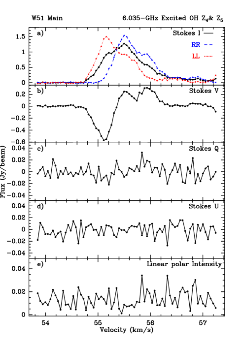
Figure 15: Same as in Fig. 12 for the Zeeman components z₄ and z₅.

*: blending of many components on the line of sight (cf. Fig. 15)
$\diamond:$ the LL counterpart of this component is quite faint and failed to pass the 3 consecutive channel criterion but the Zeeman pattern is clearly visible in the spectrum (Fig. 6). The Zeeman splitting has been consequently inferred from the Stokes $V$ spectrum.

The seven Zeeman pairs identified in this transition were used to derive a magnetic field strength ranging from $+1.6$ to $+6.8$ mG, consistent with the previously published magnetic field strengths inferred from the OH ground-state lines in the region. Note that the weak magnetic field inferred from component z₄ ($+1.6$ mG) is due to blending of components in the line of sight making this measurement less reliable.

The excited OH maser emission at 6.035 GHz shows a high degree of circular polarisation (typically $\geq 45$ % and up to 87%). Note that only one Zeeman component (z₃) shows substantial linear polarisation (30%) and has a polarisation angle $\chi=+7.1$°(Fig 7).

Figure 7: Polarisation vector associated with the elliptical Zeeman component z₃.

3.3 Comparison with ground-state OH maser emission

Fish & Reid (2007) present the distributions of the ground-state OH masers in the 1.665, 1.667 and 1.720 GHz transitions towards W51 Main/South obtained with the VLBA with a similar astrometric accuracy ($\sim$10 mas) as ours.

Figure 8 presents the 6.668-GHz methanol components and 6.035 GHz components we detected along with all the ground-state OH maser components at 1.665, 1.667 and 1.720 GHz detected by Fish & Reid (2007) in W51 Main. The ground-state OH maser emission does not alter the overall orientation along a P.A. $\simeq 70\degr$ and confirms the lanes/gaps devoid of maser emission clearly observed in the methanol maser distribution. Note that the magnetic field strengths given in Figure 8 for 1.720 GHz differ by a factor of 2 to those inferred by Fish & Reid (2007) as calculated from the Zeeman splitting coefficient given by Davies (1974) and implying potential blending of $\sigma$ components. Fish & Reid (2007) assumed that all detected 1720-MHz components were of $\sigma^{\pm 1}$ type, for which the Zeeman splitting coefficient is half that of Davies (1974). The magnetic field strengths inferred from the ground-state OH lines by Fish & Reid (2007) and from the excited OH line at 6.035 GHz (this work) are in general agreement.

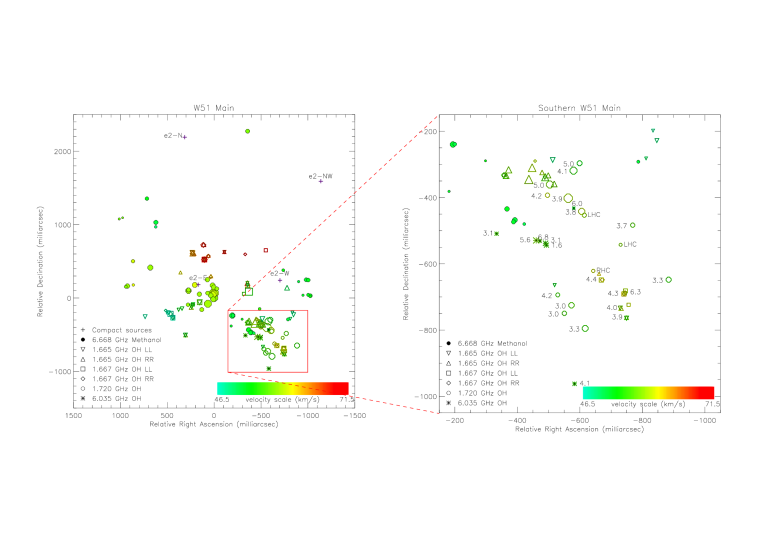
Figure 8: 6.668-GHz methanol Stokes $I$ components and 6.035 GHz Zeeman components from this work with all the ground-state OH maser components at 1.665 and 1.667 GHz in the RHC and LHC polarisations and the 1.720 GHz Zeeman pairs and isolated RHC and LHC components detected by Fish & Reid (2007) in W51 Main. The size of the symbols is proportional to the log of the intensity. The crosses indicate the positions of the compact continuum sources in the region (Shi et al. 2010a). Left panel: for the entire W51 Main region. Right panel: Magnification of the region where 6.035-GHz excited OH maser emission is found. The magnetic field associated with all Zeeman pairs in all the transitions is given by the side of each relevant component.

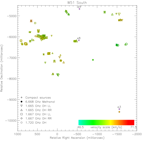
Figure 9: 6.668-GHz methanol Stokes $I$ components from this work with all the ground-state OH maser components at 1.665 and 1.667 GHz in the RHC and LHC polarisations and the 1.720 GHz Zeeman pairs and isolated RHC and LHC components detected by Fish & Reid (2007) in W51 South. The size of the symbols is proportional to the log of the intensity. The crosses indicate the positions of the compact continuum sources in the region (Gaume et al. 1993, Zhang & Ho 1997).

Considering both the methanol and OH in W51 Main, the overall maser emission seems to be centered on W51e2-E. In the northern region, covering the area $\Delta\alpha$=[+1000,+500] mas $\Delta\delta$=[+100,+1400] mas only methanol maser emission is found. In the regions centered on W51e-E and south-west of it, maser emission of both species is found, but a close look shows that methanol and OH maser components are not overlaping.

Figure 9 presents the 6.668-GHz methanol components we detected together with all the ground-state OH maser components detected by Fish & Reid (2007) in W51 South. In this region, the dichotomy between the OH and methanol maser distributions is even more pronounced. Methanol maser emission is very scarce and found in very clear distinct regions. We also note the total absence of 6.035 GHz emission and the scarcity of 1.720 GHz emission.

4 Modelling procedure

We have carried out a new parameter-space search for inversion in OH lines, up to, and including the 13-GHz transition in the ${}^{2}\Pi_{3/2},J=7/2$ rotation state. The models used the Accelerated Lambda Iteration (ALI) method to solve the coupled radiation transfer and statistical steady-state problems. The radiative transfer included only the far-infrared (FIR) transitions of OH, so it predicts only maser optical depths, without saturation or competitive propagation effects.

The model included the lowest 36 hyperfine levels of OH, coupled by 137 radiatively-allowed transitions (including the potentially maser-active hyperfine lines). Collisions of OH with both ortho- and para-H₂ were included, using the rate-coefficient from Offer & van Dishoeck (1992). The ortho- and para-H₂ ratio was 3 in the low-temperature limit, and at all model kinetic temperatures controlled by the Boltzmann distribution amongst the rotational levels of H₂. A semi-infinite slab geometry was used with 85 logarithmically-spaced slabs, covering a total depth of $3\times 10^{15}$ cm. The outer, (nearer to observer) $2\times 10^{15}$ cm, covering 80 slabs, contained OH, and had a fixed set of physical conditions (except the bulk velocity) for each model. The 5 slabs that are most remote from the observer behave as an optically thick boundary, with an exponentially increasing dust abundance, and an exponentially decreasing OH abundance. The parameter space ranges covered by the model are listed in Table 4. All models used an OH abundance of $2\times 10^{-7}$ w.r.t. H₂.

Table 4: Model parameter ranges

Parameter	Minimum value	Maximum value
Kinetic Temp.	30K	250K
Dust Temp.	10K	300K
n(H2)	106cm-3	109cm-3
$v_{microturb.}$	0 km s-1	0 km s-1
$\Delta$v	$-10$ km s-1	$+10$ km s-1

Note: All the above parameters were considered to be independent.

All the model parameters were considered to be independent. The dust parameters, for a mixture of carbonaceous and silicate dust, were taken from Draine & Lee (1984), and this was admixed with the OH-bearing slabs at an abundance of 1 per cent by mass.

Figure 10: Contour plots of maser optical depths for selected OH transitions. a, b, c show the inversion present at dust temperature T_d of 10, 72 and 134 K, respectively. The line styles for the left-hand side plots are heavy solid (1.665 GHz), dashed (1.667 GHz), light solid (1.720 GHz) and complex (1.612 GHz). The line styles for the right-hand side plots are heavy solid (6.030 GHz), dashed (6.035 GHz) and complex (4.765 GHz). Contour levels are at $\tau$=0, 0.5, 1, 2 and then doubling up to $\tau$=64. All models used an OH abundance of $2\times 10^{-7}$ w.r.t. H₂.

Figure 10: continued

In Fig. 10, we plot contours of the maser optical depth $\tau$, for notional propagation perpendicular to the slabs, and $\tau={\sum_{i}}\gamma_{i}\delta Z_{i}$, over the 80 non-boundary slabs (i=1-80), where $\gamma_{i}$ is the maser gain coefficient for the slab i. Contour levels are at $\tau$=0, 0.5, 1, 2 and then doubling up to $\tau$=64. Fig. 10a, b, c show the inversion present at dust temperature T_d of 10, 72 and 134 K, respectively. At T_d=10 K (Fig. 10a) we find that the inversions are present only for the satellite lines, and that they are weak. For the ground-state lines, the inversion zones in the OH number density, kinetic temperature (n(OH), T_K) plane for 1.612 and 1.720 GHz are distinct and significantly modified by the velocity shift, via the effects of FIR line overlaps. At T_d=72 K (Fig. 10b), the main lines appear in both the ${}^{2}\Pi_{3/2}$ J=3/2 (1.665 and 1.667 GHz) and ${}^{2}\Pi_{3/2}$ J=5/2 (6.031 and 6.035 GHz) $\Lambda$-doublets at low T_K. In general, there is little or no main-line inversion when T${}_{K}>$ T_d, which reflects the radiation-dominated pumping of these lines (Gray 2007). Peak inversions for the 6-GHz maser lines lie at larger values of n(OH) than for the 1.720-GHz line. At T_d=134 K (Fig. 10c), we can see a low density inversion region for the 1.665 and 1.667 GHz lines that is line-overlap driven. This region is absent for the 6 GHz transitions. These conclusions are in broad agreement with earlier work (Gray, Doel & Field 1991; Gray et al. 1992), but we note that these earlier parameter-space searches used the LVG approximation, and could therefore not study the important static ($\Delta$v=0) models shown in the middle row in Fig. 10a,b,c.

5 Discussion

5.1 OH and CH₃OH masers

Although not detected in these observations, maser emission in the 6.031-GHz excited transition of OH was reported by Rickard et al. (1975). The velocity range of their sole 6.031-GHz component coincides with that of the faint 6.035-GHz Zeeman pair $z_{7}$ here, which was also the strongest component detected by Rickard et al. (1975). On the other hand, the strongest 6.035-GHz component detected here, $z_{1}$, was not detected by Rickard et al. in the 1970’s. Such variability in the intensity of the maser components themselves, but also in their intensity ratios, is likely to account for the non-detection of 6.031 GHz emission here.

Overall the bulk of the methanol maser emission, both in terms of flux and number of components, is associated with W51 Main. Only two weak, isolated components are seen in W51 South, most likely associated with the e3 and e8 sources. Although the work of Fish & Reid (2007) shows that there is significant ground state OH emission from both Main and South, with indeed the brightest OH component being in South, excited OH emission is only detected towards Main.

As noted by Etoka et al. (2005) in the case of the SFR W3(OH), the present astrometric study towards W51 Main/South confirms that associations of individual OH and methanol maser components are rare. Despite all the components identified in the rich maser environment of W51 Main, no methanol and OH maser component overlap is found. The minimal separation between a ground-state OH and a methanol component is 27 mas ($\sim 150$ AU), rising to 60 mas ($\sim 300$ AU) between an excited OH and a methanol component. This is suggestive of local variations in the abundance of the species and that both species are found in closely associated, but distinct, pockets. Similarly, even though 6.035-GHz excited-OH and ground-state OH maser components are found in similar areas in W51 Main with similar magnetic field strength, they too do not show any overlap when observed at high spatial resolution.

Based on the present OH modelling results, and those of Gray et al. (1992) and Cragg et al. (2002), the total absence of 6.035-GHz emission and the scarcity of 1.720 GHz emission in W51 South, is suggestive of a lower density in W51 South than in W51 Main.

The physical conditions under which 6.668-GHz methanol masers (and 12.2-GHz methanol masers) form appears to be very similar to those that support the OH masers in almost all respects (Cragg, Sobolev & Godfrey 2005). In particular, maser optical depths are rather insensitive to the dust temperature provided the criterion $T_{d}>T_{k}$ is met, and they decay with increasing $T_{k}$ for a given dust temperature. Overall gas density also appears unable to differentiate between the OH and methanol pumping regions.

The parameter that does appear to distinguish the methanol inversion region in parameter space from that of OH is the specific column density (Cragg et al. 2005), that is the number density of the active molecule divided by the velocity gradient in the medium. Although this model cannot be applied to the middle row of Figure 10, it can be computed for the other two rows, where the velocity gradient is $5\times 10^{-11}\Delta v$ s^-1. For conditions that strongly favour 1.7-GHz to 6.0-GHz OH masers, we are restricted to number densities of OH below $\sim$10 cm^-3, or to specific column densities of less than $2\times 10^{11}/\Delta v$ s cm^-3. The models in Cragg et al. require specific optical depths of methanol that are typically a factor of ten larger. The controlling factor in which species of maser appears from a location at VLBI resolution therefore appears to be either abundance of the active molecule, or the local velocity gradient, with more quiescent gas favouring methanol over OH masers.

5.2 Distribution of masers around W51e2

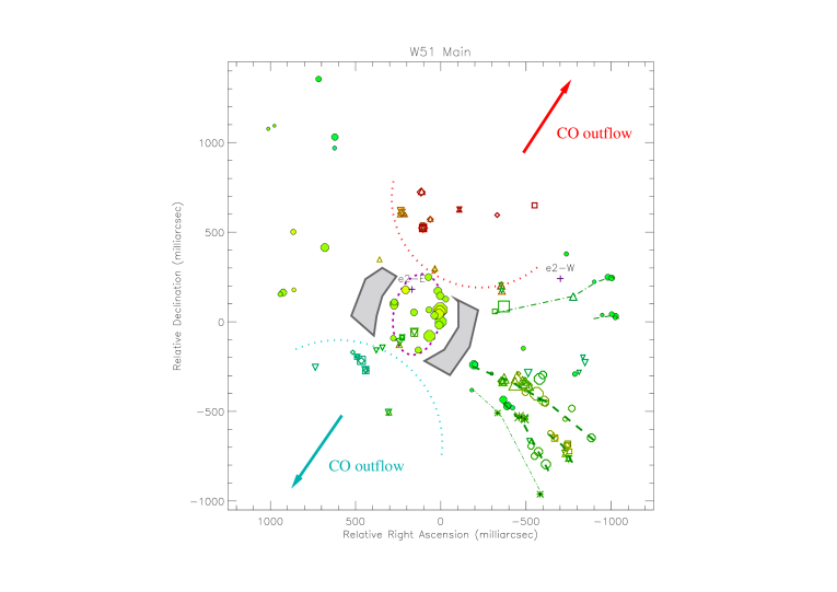
Figure 11: Magnification on the masers around e2-E and e2-W presenting the various spatial-kinematic components identified. The orientation of the CO outflow observed by Shi et al. (2010b) is indicated along with the 2 lanes/gaps (grey shaded polygons) devoid of methanol and OH maser emission. We refer to Fig. 8 for the legend.

Fig. 8 shows that there are several distinct spatial-kinematic components in the region that are identified in Fig. 11 and discussed here. The most extreme velocity maser components (within the velocity range $\sim$[+46.5,+50] km s^-1 and $\sim$[+66,+71.5] km s^-1 for the bluest and reddest components respectively), which are all ground state OH masers, lie close to a line through W51e2-E at a P.A. $\sim 150^{\circ}$ with the redshifted components north of the source and blueshifted components offset by a similar angular distance ($\sim 400$ mas) south of the source. The location of these components as well as their velocities indicate that they are associated with the outflow from the source which has been imaged by Shi et al. (2010b). Compared with these extreme velocity OH maser components, the methanol maser components, all the ground-state OH maser components at 1.720 GHz and the excited OH maser components at 6.035 GHz along with the ground-state main-line components found in the neighbouring areas (typically $\Delta\alpha\leq 0$ mas and $\Delta\delta\leq 200$ mas) have intermediate velocities.

The methanol masers are predominantly clustered within about 1″ of W51e2-E. Three major groupings separated by regions without any methanol components can be identified (Fig. 11): a number of spots east and north east of W51e2-E, a ring- or arc-like structure the centre of which is within about 200 mas of e2-E, and the remaining components which extend further to the west and southwest with a suggestion of falling into elongated structures (filaments) extending to the west or southwest and pointing back towards W51e2-E.

The majority of the excited OH masers are located at the south western edge of the methanol maser distribution, as a part of one of the most prominent filaments, extended by ground state OH masers further to the south west. The majority of the ground state OH masers trace a second, approximately parallel, filament about 100 mas north of the methanol-excited OH filament. This second prominent filament also has two methanol maser components at the eastern end, the end closest to W51e2-E.

The spatial segregation of the maser species around W51e2-E as well as the lack of overlap of components from different species, plus the extreme difference in the richness of the methanol maser emission towards W51 Main and South, both point to significant variations in the physical and chemical conditions in the region as has been noted previously by Fish & Reid (2007).

5.3 Polarisation and magnetic field

The magnetic field strengths inferred here from the 6.035-GHz excited OH Zeeman components range from $\sim+2$ mG to $\sim+7$ mG (Table 3), consistent with the 4.1 mG reported by Rickard et al. (1975) from the 6.031-GHz excited OH transition and inferred from the ground state OH transitions as discussed in section 3.3.

Polarisation angle measurements have been obtained towards W51e2 by Lai et al. (2001) from BIMA 1.3-mm dust continuum observations, further analysed by Tang et al. (2009). The polarisation angle they measure in the region where the elliptical OH Zeeman component z₃ emanates from, is in agreement with the polarisation angle we measure. Tang et al. (2009) conclude from the analysis of the overall polarisation angle distribution for the BIMA observations at 1.3-mm that the magnetic field has an hourglass morphology pinched along a plane consistent with the H53$\alpha$ accretion flow proposed by Keto & Klaassen (2008). The orientation of the proposed flow (P.A. $\simeq 60\degr$) is consistent with the distribution of the intermediate velocity maser population (P.A. $\simeq 70\degr$). We also note that the orientation of the filamentary structures observed in the southwestern regions (cf. section 5.2) seems also in agreement with the magnetic field line directions inferred by Tang et al. (2008) for this region and given in their $B$-field maps (their Fig. 5). This seems to indicate that the maser features are likely to be part of a flow in which the dynamics are magnetically dominated, so that motion along the field lines is significantly easier than accross them. The filamentary structure orientation can be explained if the maser spots trace the magnetic field lines.

5.4 Interpretation and scenarios

Fig. 3b presents the velocity distribution of the methanol maser spots versus radial distance. The figure shows that the red- and blue-shifted maser components are diverging from a common point with an expansion velocity of $\simeq$5 km s^-1. This, added to the general distribution of the methanol maser components in the plane of the sky (Fig. 3a & Fig. 11), indicates the presence of a structure with a wide opening angle centred on W51e2.

We can estimate roughly the total mass traced by the structure from the material that would be contained by the enclosing sphere. With a total extent of $\sim$1.5″ and assuming n(H₂)=$5\times 10^{7}$cm^-3 from the OH modelling of the region, the upper limit for the total mass is 90 M_⊙. An estimate of the lower limit can be obtained by considering only the volume strictly traced by the methanol masers. Considering the $\sim 45\degr$ opening angle of the structure, translating into a filling factor of 0.25, gives us 22.5 M_⊙.

Scenario 1: Outflow
One possible interpretation for the wide-opening angle structure observed is the presence of an outflow.

According to Churchwell (2002), typically an outflow from a high-mass young stellar object (HMYSO; i.e., L${}_{bol}>10^{3}$ L_⊙) lives $\sim 10^{4}$ yr with a mass outflow rate of $\sim 10^{-3}$ M_⊙ yr^-1. With an expansion velocity of 5 km s^-1, only $\sim 5\times 10^{3}$ year would be needed to reach 1″, corresponding to the extent of the red- and blue shifted lobe observed in Fig. 3a.

Considering this time scale and the lower and higher total mass limits inferred here, this would lead to an outflow rate of $\simeq 2\times 10^{-2}\rightarrow 4\times 10^{-3}$ M_⊙ yr^-1. This is quite similar to the mass outflow rate inferred by Shi et al. (2010b) for the CO outflow observed perpendicular to the wide-angle structure traced by the masers.

In this scenario, the 2 gaps observed in the distribution of the masers could be explained by 2 episodic events. The ring-like structure closest to e2-E, well defined by an ellipse of long-axis $\sim 220$ mas, would trace an outflow event $\sim 1.1\times 10^{3}$ yr old only, assuming no acceleration or deceleration.

Scenario 2: Accreting flow
The northeast-southwest distribution of the masers is close to perpendicular to the axis of the well collimated outflow of material imaged in CO by Shi et al. (2010b). This suggests that alternatively the masers could be tracing material which is part of the static or infalling envelope around the forming star.

The excitation models show that both OH and methanol maser emission are suppressed by higher gas temperatures. This could provide an explanation for the gaps which separate the two outer groups of methanol masers from the central cluster. Closer to the central source the gas is likely to be hotter and so maser emission is suppressed, even if there is a high abundance of methanol and OH. Alternatively, the gaps could reflect regions where the infall velocity increases, destroying the velocity coherent path along the line of sight necessary for maser amplification.

The methanol masers closest to e2-E, forming a compact ring-like structure, likely trace a distinct physical component. Similar structures are seen by Bartkiewicz et al. (2009) towards some 29% of the 6.7-GHz methanol maser sources they studied. They interpreted these as a result of the masers being associated with a dense disk or torus around the central source, an interpretation which could also be applied to the masers seen here. The fact that these masers exhibit similar red-shifted velocities as the masers located $\sim 1\arcsec$ north-east of e2-E could be due to radiative transfer effects in the infalling envelope.

5.5 Stage of evolution and properties of the sources

Masers have been proposed as tracers of the evolutionary stage of HMYSOs which excite them. For example Breen et al. (2010) propose a scheme in which sources evolve from exciting only methanol masers to having both methanol and OH masers while their UCHII region grows. Subsequently, the methanol maser emission ceases leaving OH masers associated with the star and its UCHII region. Within such a scheme these observations of W51 Main and South suggest that the methanol-poor South region is more evolved than the much more methanol-rich Main region. In South, the ground-state OH masers appear primarily associated with UCHII region e8. Both the methanol and OH masers in Main are associated with the presumably younger dust continuum dominated source e2-E with little evidence that indicates any of the masers are associated with the UCHII region e2-W.

Shi et al (2010a) propose that there is either a single O protostar or a cluster of B stars at the centre of W51e-E. The results of Keto & Klaassen (2008) and Shi et al. (2010b) seems to indicate that there are 2 possible HMYSO in the W51e2 region: W51e2-E and W51e2-W. Shi et al. (2010b) reach the conclusion that W51e2-W is somewhat older than W51e2-E and was formerly the active centre of the region but has now ceased to accrete and that it is now W51e2-E which dominates the gas accretion in the W51e2 molecular core. The presence of the methanol wide-opening angle structure with no UCHII region association points to the existence of a O-protostar in the early stage of evolution in the cluster.

Interferometric observations of methyl cyanide towards the W51 Main and South region by Remijan et al. (2004) identified hot gas associated with e2 and e1, although the observations had insuffient resolution to separate the components of e2. At the $2\arcsec-3\arcsec$ resolution of the observations the e2 and e1 regions were resolved with the lines peaking at a velocity of 56 km s^-1 towards e1 and 53 km s^-1 towards e2. Many of the lines are optically thick but correcting for this, the analysis found e1 and e2 to have similar temperatures ($\sim 130$K), methyl cyanide column densities (few$\times 10^{16}$cm^-2) and hydrogen volume densities ($\sim 5\times 10^{5}$cm^-3). However, contrary to what might be expected on the basis of these methyl cyanide results, there are no maser components associated with the e1 source. The masers in the south are associated with e8, except for the lone methanol component associated with e3. Whether this difference between the masers and the hot methyl cyanide reflects a difference in the evolutionary status of the e1 and e8 sources is unclear, but higher resolution observations of both the thermal line emission and the dust continuum emission from this region would provide important insights into this question.

5.6 Comparison with similar SFR complexes

Studies of the 6-GHz excited-state OH and 6.668-GHz methanol maser emission with similar astrometric accuracy to those presented here have also been performed towards the SFR complexes W3(OH) (Etoka et al. 2005) and ON1 (Green et al. 2007). The results in ON1 are remarkably similar to W51. In particular, in ON1 there is no association between 6-GHz excited-state OH and methanol masers with the closest components of each species being separated by $\sim$23 mas. In addition, the 6-GHz excited-state OH and methanol masers form a linear distribution. However this structure is systematically offset (by $\sim$60-70 mas) from another linear distribution traced by ground-state OH masers. This offset could result from the proper motions of the masers in the 9 years between the observations of the ground-state OH (Nammahachak et al. 2006) and the methanol and 6-GHz excited-state OH. Nonetheless, this filamentary distribution is strikingly reminiscent of that observed here in the south-southwest part of W51 Main. In addition, the magnetic field measured in ON1 is similar in strength to that in W51. These similarities suggest a similar mechanism/environment is observed in both SFR complexes.

In contrast, the maser distribution in W3(OH) is quite different from W51 or ON1. Even though long filamentary structures are observed, the most striking one being the large-extended filament traced both by 6.668-GHz methanol and 4.765-GHz excited-OH maser emission (Harvey-Smith & Cohen 2006), there is no clear apparent pattern nor segregation of the different species in the area probed by the maser components.

6 Summary and conclusion

We have presented MERLIN astrometric observations towards W51 Main and South of the Class II methanol maser emission at 6.668 GHz and the excited OH maser emission at 6.035 GHz. The 6-GHz maser distributions have been aligned with those of the ground-state OH maser transitions at 1.665, 1.667 and 1.720 GHz from Fish & Reid (2007). Although Main and South have similar number of OH ground-state maser components with the strongest component in South, the bulk of the methanol 6.668 GHz maser emission, and all of the excited OH 6.035 GHz maser emission are found to be associated with e2 in W51 Main. Only two faint methanol maser spots are found in W51 South, probably associated with e3 and e8. Modelling implies n(H₂)$\simeq 5\times 10^{7}$cm^-3, a dust temperature 30 K$\leq$ T${}_{d}\leq$130 K and a kinetic temperature T${}_{K}\leq$T_d as reasonable physical conditions for Main with a possibly lower density for South.

At this high spatial resolution (better than 15 mas), no overlapping of OH and methanol maser spots or 6.035-GHz excited-OH and ground-state OH maser components are found even in the most crowded areas.

The alignment of the 18-cm ground-state masers and the 5-cm methanol and excited OH masers also reveal that the extreme velocity main-line masers found $\simeq$400 mas north and south of e2-E (either side of the methanol ring-like struture) are associated with the well-known outflow observed in CO by Shi et al. (2010b).

The masers in the south-southwest region of W51 Main clearly exhibit a filamentary structure. Those filaments extend west or southwest and point back towards e2-E. There are 2 prominent filaments, one of which contains the bulk of the 6.035-GHz maser spots, located at the southwest edge of the methanol maser spots and extended by 1.720-GHz maser spots. The magnetic strength and direction inferred from the excited OH maser emission at 6.035 GHz is in agreement with former measurements in the region. Also, our measured polarisation angle is in agreement with BIMA 1.3-mm observations, interpreted by Tang et al. (2009) as the signature of an hourglass magnetic field structure suggesting that the maser spots trace the magnetic field lines.

A close inspection of the methanol masers revealed a wide-opening angle structure centred on e2-E, roughly aligned on a P.A.$\sim 150\degr$, that is roughly perpendicular to the CO outflow, and showing a clear velocity coherence. We estimated that the mass in this structure is between 22.5 and 90 M_⊙. The two possible interpretations of this structure are the signature of (1) an outflow showing episodic events of $\sim 5\times 10^{3}$ yr for the older event and $\sim 1\times 10^{3}$ yr for the younger one, assuming an outflow velocity of $\sim~{}5$ km s^-1 or; (2) an accretion flow in which two physical components are present: an infalling anvelope with the central ring-like structure probing a compact and dense disk or torus around the central object.

Although e2-W is the only continuum source in W51e2 clearly associated with a UCHII region, currently e2-E seems to be the most active source in the region. The presence of methanol masers and the lack of a UCHII region point at a massive central object at an early stage of the star forming process.

Appendix A Spectra for the 6.035-GHz excited OH Zeeman components

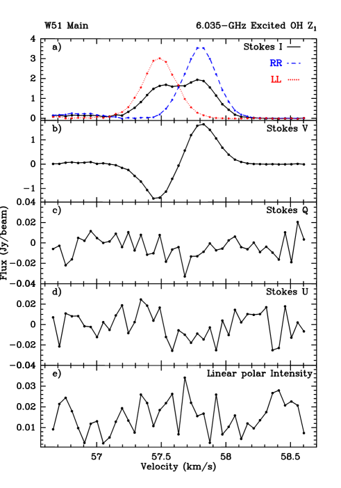
Figure 12: Spectra of the Zeeman component z₁ (6.035-GHz excited OH line). a) Stokes $I$, RHC and LHC spectra. b) Stokes $V$. c) Stokes $Q$. d) Stokes $U$. e) linear polarisation intensity $P$.

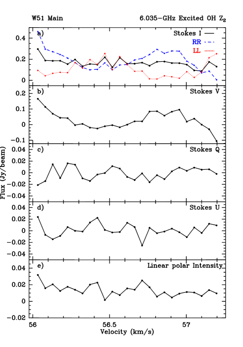
Figure 13: Same as in Fig. 12 for the Zeeman component z₂. Note that the velocity range presented here encompass exclusively that of the component due to contamination by other components in the adjacent channels. This is the reason why the wings do not return to zero.

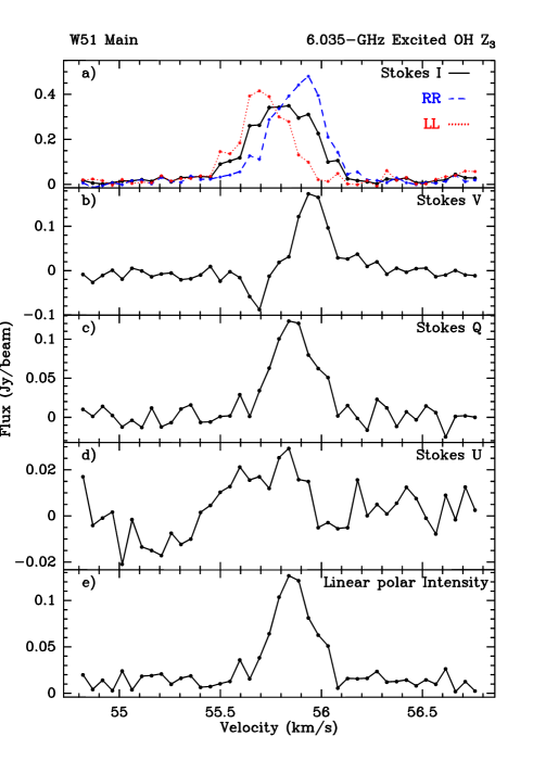
Figure 14: Same as in Fig. 12 for the Zeeman component z₃.

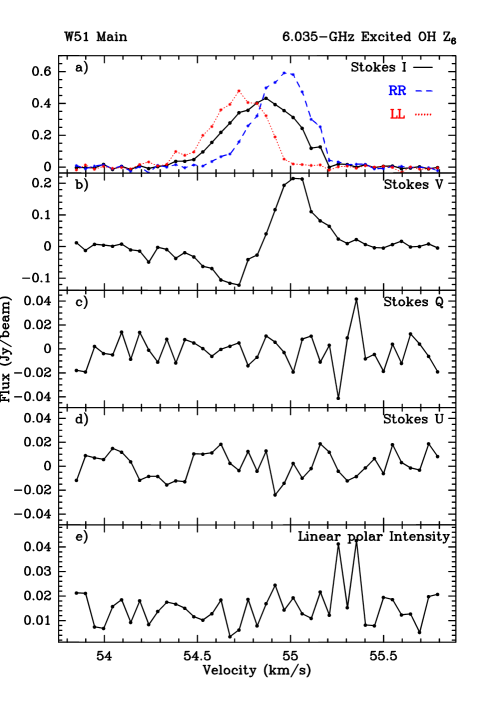
Figure 16: Same as in Fig. 12 for the Zeeman component z₆

References

- [Avison2010] Avison A., 2010 PhD thesis, The University of Manchester
- [Bartkiewicz et al.2009] Bartkiewicz A., Szymczak M., van Langevelde H.J., Richards A.M.S. & Pihlström Y.M., 2009, A&A, 502, 155
- [Breen et al2010] Breen S.L., Ellingsen S.P., Caswell J.L. & Lewis B.E., 2010, MNRAS, 401, 2219
- [Baudry et al.1997] Baudry A., Desmurs J.F., Wilson T.L. & Cohen R.J., 1997, A&A, 325, 255
- [Carpenter and Sanders1998] Carpenter J.M. & Sanders D.B., 1998, AJ, 116, 1856
- [Caswell2003] Caswell J.L., 2003, MNRAS, 341, 551
- [Caswell and Vaile1995] Caswell J.L. & Vaile R.A., 1995, MNRAS, 273, 328
- [Churchwell2002] Churchwell E., 2002, ARA&A, 40, 27
- [Cragg et al22005] Cragg D.M., Sobolev A.M. & Godfrey P.D., 2005, MNRAS, 360, 533
- [Cragg et al12002] Cragg D.M., Sobolev A.M. & Godfrey P.D., 2002, MNRAS, 331, 521
- [Diamond et al2003] Diamond P.J., Garrington S.T., Gunn A.G., Leahy J.P., McDonald A., Muxlow T.W.B., Richards A.M.S. & Thomasson P., 2003, MERLIN User Guide, v. 3
- [Davies1974] Davies R.D., 1974, IAUS, 60, 275
- [Desmurs and Baudry1998] Desmurs J.-F. & Baudry A., 1998, A&A, 340, 521
- [Draine and Lee1984] Draine B.T. & Lee H.M., 1984, ApJ, 285, 89
- [Etoka etal2005] Etoka S., Cohen R.J. & Gray M.D., 2005, MNRAS, 360, 1162
- [Fish and Reid2007] Fish V.L. & Reid M.J., 2007, ApJ, 670, 1172
- [Gaume etal1993] Gaume R.A., Johnston K.L. & Wilson T.L., 1993, ApJ 417, 645
- [Genzel et al11981] Genzel R., et al., 1981, ApJ, 247, 1039
- [Genzel et al21978] Genzel R., et al., 1978, A&A, 66, 13
- [Gray et al11991] Gray M.D., Doel R.C. & Field D., 1991, MNRAS, 252, 30
- [Gray et al11992] Gray M.D., Field D. & Doel R.C., 1992, A&A, 262, 555
- [Gray2007] Gray M.D., 2007, MNRAS, 375, 477
- [Green et al2007] Green J.A., Richards A.M.S., Vlemmings W.H. T., Diamond P. & Cohen R.J., 2007, MNRAS, 382, 770
- [Harvey-Smith and Cohen2006] Harvey-Smith L. & Cohen, R.J, 2006, MNRAS, 371, 1550
- [Imai et al2002] Imai H., et al., 2002, PASJ, 54, 741
- [Jaffe et al1987] Jaffe D.T., Harris A.I. & Genzel R., 1987, ApJ, 316, 231
- [Kalenskii and Johansson2010] Kalenskii S.V. & Johansson L.E.B., 2010, A Rep, 54, 1084
- [Keto2008] Keto E. & Klaasen P., 2008, ApJ, 678, L109
- [Nammahachak et al2006] Nammahachak S., Asanok K., Hutawarakorn Kramer, B., Cohen R.J., Muanwong O., Gasiprong N., 2006 MNRAS 371, 619
- [Merhinger1994] Merhinger D.M., 1994, ApJS, 91, 713
- [Lai et al2001] Lai S.-P., Crutcher R.M., Girart J.M. & Rao R., 2001, ApJ, 561, 864
- [Menten et al21990] Menten K.M., Melnick G.J. & Phillips T.G., 1990, ApJ, 350, L41
- [Menten etal21990] Menten K.M., Melnick G.J., Phillips T.G. & Neufeld D.A., 1990, ApJ, 363, L27
- [Mufson and Liszt1979] Mufson S.L., & Liszt H.S., 1979, ApJ, 232, 451
- [Offer and van Dishoeck1992] Offer A.R. & van Dishoeck E.F., 1992 MNRAS, 257, 377
- [Pavlakis and Kylafis2000] Pavlakis K.G. & Kylafis N.D., 2000, ApJ, 534, 770
- [Phillips2005] Phillips C. & van Langevelde H., 2005, ASPC, 340, 342
- [Rickard et al.1975] Rickard L.J., Zuckerman B. & Palmer B., 1975, ApJ, 200, 6
- [Remijan etal12004] Remijan A., Sutton E.C., Snyder L.E., Friedel D.N., Liu S.-Y. & Pei C.-C., 2004, ApJ, 606, 917
- [Rudolph et al1990] Rudolph A., Welch, W.J., Palmer P., & Dubrulle B., 1990, ApJ, 363, 528
- [Sato et al2010] Sato M., Reid M.J., Brunthaler A. & Menten K.M., 2010, ApJ, 720, 1055
- [Shi et al12010] Shi H., Zhao J.-H. & Han J.L., 2010a, ApJ, 710, 843
- [Shi et al12010] Shi H., Zhao J.-H. & Han J.L., 2010b, ApJ, 718L, 181
- [Sollins et al 2004] Sollins P.K., Zhang Q. & Ho P.T.P., 2004, ApJ, 606, 943
- [Tang et al2009] Tang Y.-W., Ho P.T.P., Koch P.M., Girart J.M., Lai S.-P. & Rao R., 2009, ApJ, 700, 251
- [ Westerhout1958] Westerhout G., 1958, Bull. Astron. Inst. Netherlands, 14, 215
- [Zhang etal11997] Zhang Q. & Ho P.T.P., 1997, ApJ, 488, 241
- [Zhang etal21998] Zhang Q., Ho P.T.P., & Ohashi N., 1998, ApJ, 494, 636