Random pinning limits the size of membrane adhesion domains

Abstract

Theoretical models describing specific adhesion of membranes predict (for certain parameters) a macroscopic phase separation of bonds into adhesion domains. We show that this behavior is fundamentally altered if the membrane is pinned randomly due to, e.g., proteins that anchor the membrane to the cytoskeleton. Perturbations which locally restrict membrane height fluctuations induce quenched disorder of the random-field type. This rigorously prevents the formation of macroscopic adhesion domains following the Imry-Ma argument [Y. Imry and S. K. Ma, Phys. Rev. Lett. 35, 1399 (1975)]. Our prediction of random-field disorder follows from analytical calculations, and is strikingly confirmed in large-scale Monte Carlo simulations. These simulations are based on an efficient composite Monte Carlo move, whereby membrane height and bond degrees of freedom are updated simultaneously in a single move. The application of this move should prove rewarding for other systems also.

I Introduction

The fate of living cells is regulated through interactions with other cells and with the extracellular matrix (ECM). Through receptor-ligand bonds formed by specific proteins the cell adheres to the ECM forming adhesion domains (clusters of closed bonds). Not all adhesion domains are focal adhesions but these are particularly well studied and relevant. Focal adhesions are involved in the transmission of signals and mechanical forces, and play key roles in cell anchorage and migration Geiger et al. (2001); Parsons et al. (2010). Consequently, understanding how adhesion domains form, and the factors that control their size, shape, and growth Nicolas et al. (2004); Gov (2006), is of profound practical importance. Extensive studies have been performed on theoretical models for single bond dynamics Bell (1978), collective dynamics of discrete bonds Weikl et al. (2002); Krobath et al. (2007); Speck et al. (2010); Weil and Farago (2010); Farago (2011), and employing effective potentials Lipowsky (1996); Zhang and Wang (2008); Atilgan and Ovryn (2009); as well as experimentally on cell-mimetic model systems Tanaka and Sackmann (2005); Mossman and Groves (2007) such as lipid bilayer vesicles with embedded ligands brought in the vicinity of receptors tethered to supported membranes Bruinsma et al. (2000); Cuvelier and Nassoy (2004); Reister-Gottfried et al. (2008); Limozin and Sengupta (2009); Smith and Sackmann (2009).

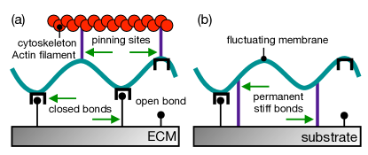
Figure 1: (Color online) Sketch of two typical situations in which the formation of macroscopic adhesion domains is prevented due to the presence of random fields: (a) A membrane of a biological cell adheres to the ECM via receptor-ligand bonds, which may dynamically open and close. The membrane is freely fluctuating except at the anchoring sites (pinning sites) attaching the membrane to the cytoskeleton. (b) An analogous in vitro example in which the pinning sites are formed by stiff and permanently closed bonds (tethers) between membrane and substrate.

While theoretical models predict a macroscopic phase separation, adhesion domains in cells are typically finite in size. It has been proposed that trapping in membrane corrals (or compartments) reduces the mobility of receptors Kusumi et al. (2005), which becomes a limiting factor for the growth of adhesion domains. The purpose of this paper is to provide an alternative explanation based on the observation that, due to the interactions with the ECM, membrane height fluctuations are locally suppressed. These “pinning sites” induce quenched disorder of the random-field type which prevents macroscopic domain formation in $d=2$ dimensions Imry and Ma (1975); Imbrie (1984); Bricmont and Kupiainen (1987); Aizenman and Wehr (1989). Hence, based on the fundamentals of statistical physics alone, adhesion domains of finite size are implied in a wide variety of contexts. The mere presence of random-field disorder provides a robust mechanism controlling the size of adhesion domains, irrespective of the details of the many and complex molecular processes between cell and ECM.

The generic situation that we envision is sketched in Fig. 1(a), which shows a fluctuating membrane adhering to a substrate via receptor-ligand bonds. The crucial ingredients are the pinning sites at which the membrane height is assumed to be fixed. In a biological cell, such pinning sites correspond, e.g., to the locations where the cytoskeleton anchors to the membrane. For an experimental verification of our predictions in vitro we propose a bilayer adhered to a substrate or supported membrane with a (small) fraction of the receptor-ligand bonds permanently closed and of high stiffness [Fig. 1(b)]. We will show that in situations resembling those of Fig. 1 adhesion domains remain finite in size for any finite concentration of pinning sites, provided the spatial distribution of pinning sites is random.

II Model

To show how the random-field disorder in the specific adhesion of membranes comes about we consider a class of simple models as reviewed in Ref. Weikl and Lipowsky, 2007. These coarse-grained models contain the minimal ingredients that we require to address the influence of membrane pinning on the statistics of adhesion domain formation. In particular, we assume the membrane to be a two-dimensional sheet characterized by a bending rigidity, and to be in thermal equilibrium with its surroundings. The ligand-receptor bonds and pinning sites are treated as point particles. We neglect all active processes and, in the case of focal adhesions, the influence that stresses applied to the substrate may have on the development of adhesion domains Nicolas et al. (2004).

In the Monge representation a membrane patch with projected area $A=L^{2}$ is described through its separation profile $h(\mathbf{r})$ describing the height of the membrane at position $\mathbf{r}=(x,y)$, $0\leqslant x,y<L$, measured with respect to some (arbitrarily chosen) reference height. The effective Hamiltonian reads

$$\mathcal{H}_{0}[h(\mathbf{r})]=\int_{A}\mathrm{d}^{2}\mathbf{r}\;\left\{\frac{\kappa}{2}[\nabla^{2}h(\mathbf{r})]^{2}+\frac{\gamma}{2}[h(\mathbf{r})]^{2}\right\}.$$ (1)

The first term governs the bending energy, with $\kappa$ the membrane bending rigidity, which we assume is the dominant contribution to the Helfrich energy Helfrich (1978). The second term is the lowest-order expansion of the non-specific interactions between membrane and substrate whose strength is denoted $\gamma$. In our treatment, the minimum of the non-specific potential is thus taken to be the reference height from which $h(\mathbf{r})$ is measured. These non-specific interactions arise due to volume exclusion, van der Waals forces, and the possible formation of an electrostatic double layer, as well as an effective pressure due to the restricted volume the membrane can move in.

The parameters $\kappa$ and $\gamma$ define a length, $\xi_{\parallel}\equiv(\kappa/\gamma)^{1/4}$, which sets the scale over which the membrane height fluctuations are correlated Speck et al. (2010),

$$m(|\mathbf{r}-\mathbf{r}^{\prime}|)\equiv\langle h(\mathbf{r})h(\mathbf{r}^{\prime})\rangle_{0}\approx\xi_{\perp}^{2}u(|\mathbf{r}-\mathbf{r}^{\prime}|/\xi_{\parallel}),$$ (2)

see appendix A. The scaling function is defined in terms of the Kelvin function, $u(x)=-(4/\pi)\,{\rm kei}_{0}(x)$; it obeys $u(0)=1$ and decays to zero exponentially fast. The amplitude of the correlations is set by the thermal roughness $\xi_{\perp}\equiv\xi_{\parallel}/\sqrt{8\beta\kappa}$, $\beta\equiv(k_{\text{B}}T)^{-1}$, with temperature $T$ and Boltzmann constant $k_{\text{B}}$. The brackets $\langle\cdots\rangle_{0}$ denote the thermal average with respect to the Hamiltonian Eq. (1), i.e., in the absence of ligand-receptor bonds and pinning sites.

Now imagine a set of $N$ receptor-ligand pairs at positions $R\equiv\{\mathbf{r}_{1},\mathbf{r}_{2},\ldots,\mathbf{r}_{N}\}$ embedded in the membrane and substrate that can form bonds. The arguably simplest model is to assign a linear energy to closed bonds with stiffness $\alpha$ Weikl et al. (2002). The total Hamiltonian then reads

$$\mathcal{H}_{N}=\mathcal{H}_{0}+\sum_{i=1}^{N}b_{i}[\alpha h(\mathbf{r}_{i})-\varepsilon_{\text{b}}],$$ (3)

where $b_{i}=0$ if the $i$th bond is open, and $b_{i}=1$ if the bond is closed. The parameter $\varepsilon_{\text{b}}=\varepsilon_{\text{b}}^{0}-\alpha d$ is the shifted binding energy the system gains through forming a bond, where $\varepsilon_{\text{b}}^{0}$ is the bare binding energy and $d$ is the separation between substrate and the minimum of the non-specific potential. In addition to the receptor-ligand pairs, we assume the presence of $n$ pinning sites at positions $P\equiv\{\mathbf{r}_{N+1},\ldots,\mathbf{r}_{M}\}$ where the membrane height is fixed to $h=h_{\text{P}}$. We take the two sets $R$ and $P$ to be disjoint with their union thus holding $M=N+n$ distinct sites.

III Theoretical mapping

We now calculate the free energy as a function of the bond variables $\{b_{i}\}$ through integrating out the height fluctuations under the constraints $h(\mathbf{r}_{i})=h_{i}$ for sites $\mathbf{r}_{i}\in R$ and $h(\mathbf{r}_{i})=h_{\text{P}}$ for $\mathbf{r}_{i}\in P$. We follow the standard procedure and implement these $M$ constraints through $\delta$-functions Li and Kardar (1991); for the detailed calculation see appendix B.

For clarity of the presentation, in the following we consider the case $h_{\text{P}}=0$. The free energy then reads

$$G(\{b_{i}\};R\cup P)=-\beta^{-1}\ln\int\mathrm{d}h_{1}\cdots\mathrm{d}h_{N}\;\times\\ \exp\left\{-\frac{1}{2}\sum_{i,j=1}^{N}(\mathsf{m}^{-1})_{ij}h_{i}h_{j}-\beta\sum_{i=1}^{N}b_{i}[\alpha h_{i}-\varepsilon_{\text{b}}]\right\}.$$ (4)

The dependence on the positions $R$ and $P$ is encoded in the matrix $\mathsf{m}$, whose components are given by $m_{ij}\equiv m(|\mathbf{r}_{i}-\mathbf{r}_{j}|)$. Performing the final integrations we obtain

$$G=-\sum_{i=1}^{N}\sum_{j=i+1}^{N}\varepsilon_{ij}b_{i}b_{j}-\sum_{i=1}^{N}\mu_{i}b_{i},\quad\varepsilon_{ij}\equiv\beta\alpha^{2}\hat{m}_{ij},$$ (5)

with $\mu_{i}\equiv\varepsilon_{\text{b}}+\beta\alpha^{2}\hat{m}_{ii}/2$, and where we have introduced a new matrix $\hat{\mathsf{m}}$. While Eq. (4) contains the full matrix $\mathsf{m}$, the sums run only over the first $N$ sites corresponding to the bonds and excluding the pinning sites. The matrix $\hat{\mathsf{m}}$ is obtained by inverting the submatrix formed by the first $N$ rows and $N$ columns of $\mathsf{m}^{-1}$. Note also that we have dropped an additional term in Eq. (5) which depends on the geometry of both the bonds and the pinning sites but not on the state $\{b_{i}\}$ of the bonds.

The key result here is that the free energy in Eq. (5) is isomorphic to the Ising lattice gas with couplings $\varepsilon_{ij}\propto\alpha^{2}$ and a site-dependent effective chemical potential $\mu_{i}$ that also depends on the stiffness $\alpha$. There are two effects due to membrane undulations: First, single bond formation is assisted ($\mu_{i}>\varepsilon_{\text{b}}$) since the system can access configurations with lower energy. Second, bonds couple in a manner that enhances clustering: a closed bond pulls down the membrane locally making it easier for nearby bonds to also close. In such bound patches (adhesion domains) membrane fluctuations are hindered and, therefore, the entropy is decreased. The phase behavior of the system is thus determined by the competition between this loss of entropy, the mixing entropy of bonds, and the gain in binding energy. For small $\xi_{\parallel}$ only nearest neighbors interact directly; by increasing $\xi_{\parallel}$ (i.e., for stiffer membranes) the thermal roughness $\xi_{\perp}$ determining the strength of the coupling is diminished but more and more bonds become coupled.

III.1 Membrane without pinning

The result Eq. (5) holds for any geometry of bonds and pinning sites. In the absence of pinning sites ($n=0$) clearly $\hat{\mathsf{m}}=\mathsf{m}$ and the chemical potential becomes spatially uniform, $\mu_{i}=\varepsilon_{\text{b}}+\varepsilon_{0}/2\equiv\mu_{0}$, where

$$\varepsilon_{0}\equiv\beta(\alpha\xi_{\perp})^{2}=\alpha^{2}/(8\sqrt{\kappa\gamma})$$ (6)

is the effective coupling energy due to the membrane undulations. We now specialize to the situation where the positions $R$ of receptor-ligand pairs form a regular square lattice with lattice spacing $a\sim\xi_{\parallel}$. The phase behavior in this case is known Lipowsky (1996); Weikl et al. (2002): For sufficiently high $\alpha>\alpha^{\ast}$ there is a first order phase transition from a bound state ($\phi\sim 1$) with a high density of closed bonds

$$\phi\equiv\frac{1}{N}\sum_{i=1}^{N}b_{i}\quad,$$ (7)

to an unbound state with a low density of closed bonds ($\phi\sim 0$). Precisely at $\alpha=\alpha^{\ast}$ the system shows critical behavior which, by virtue of the mapping of Eq. (5), belongs to the universality class of the $d=2$ Ising model.

III.2 The pinned membrane

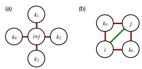
Figure 2: (Color online) Graphical aid to identify the non-vanishing components of the matrices $\widehat{{\mathsf{A}}^{2}}$ and ${\hat{\mathsf{A}}}^{2}$ appearing in Eq. (9) with bond sites $i$ and $j$: (a) For $i=j$ the sites $k_{1},\dots,k_{4}$ that are nearest neighbors of $i$ are counted. (b) For the case that $i$ and $j$ are next-nearest neighbors the sites $k_{5}$ and $k_{6}$ that are common nearest neighbors of both $i$ and $j$ are counted.

We now come to the main result of this paper, where the fate of the mapping of Eq. (5) in the presence of pinning sites $(n>0)$ is considered. In this case, we must distinguish between the set $R$ of sites where receptor-ligand bonds may form, and the set $P$ of sites at which the membrane is pinned. We furthermore restrict our calculation of $\hat{\mathsf{m}}$ to nearest and next-nearest neighbor interactions. We first write $\mathsf{m}=\xi_{\perp}^{2}[\mathbf{1}+\epsilon_{\text{A}}\mathsf{A}+\epsilon_{\text{B}}\mathsf{B}]$, where the $M\times M$ matrices $\mathsf{A}$ and $\mathsf{B}$ correspond to nearest and next-nearest neighbor interactions, respectively. The components $A_{ij}$ ($B_{ij}$) equal one if the two sites $i$ and $j$ are nearest (next-nearest) neighbors, and zero otherwise. The coefficients are set by the value of the scaling function at the nearest and next-nearest neighbor distance, $\epsilon_{\text{A}}\equiv u(a/\xi_{\parallel})$ and $\epsilon_{\text{B}}\equiv u(\sqrt{2}a/\xi_{\parallel})$, respectively. We expand the inverse as

$$(\mathsf{m}/\xi_{\perp}^{2})^{-1}\approx\mathbf{1}-\epsilon_{\text{A}}\mathsf{A}-\epsilon_{\text{B}}\mathsf{B}+\epsilon_{\text{A}}^{2}\mathsf{A}^{2},$$ (8)

where all terms with coefficients $<\epsilon_{\text{A}}^{2}$ have been dropped. We now replace, in Eq. (8), the $M\times M$ matrices $\{\mathbf{1},\mathsf{A},\mathsf{B}\}$ by the $N\times N$ sub-matrices $\{\hat{\mathbf{1}},\hat{\mathsf{A}},\hat{\mathsf{B}}\}$ obtained by discarding the $n$ upper rows and columns corresponding to pinning sites; taking the inverse of the resulting matrix yields the desired matrix $\hat{\mathsf{m}}$ that appears in the mapping of Eq. (5)

$$\hat{\mathsf{m}}/\xi_{\perp}^{2}\approx\hat{\mathbf{1}}+\epsilon_{\text{A}}\hat{\mathsf{A}}+\epsilon_{\text{B}}\hat{\mathsf{B}}+\epsilon_{\text{A}}^{2}\left({\hat{\mathsf{A}}}^{2}-\widehat{{\mathsf{A}}^{2}}\right),$$ (9)

where all higher order terms have again been dropped.

Due to the pinning sites, the last term in Eq. (9) does not vanish since the “hat” and “square” operations do not commute. First we evaluate $(\widehat{{\mathsf{A}}^{2}})_{ij}=\sum_{k=1}^{M}A_{ik}A_{kj}$ where, in the summation, only two terms survive (Fig. 2). The first term corresponds to $i=j$; a non-zero contribution implies that $k$ needs to be a nearest neighbor of this site. On a square lattice there are four such sites labeled $k_{1},\dots,k_{4}$ in Fig. 2(a). The second term arises when $i$ and $j$ are distinct. The only combination with a non-zero contribution is when $i$ and $j$ are both nearest-neighbor of the same site $k$, which implies that $i$ and $j$ are next-nearest neighbors. Two such sites can be identified, labeled $k_{5}$ and $k_{6}$ in Fig. 2(b). Hence,

$$(\widehat{{\mathsf{A}}^{2}})_{ij}=4\delta_{ij}+2B_{ij},$$ (10)

with $\delta_{ij}$ the Kronecker symbol. The components of the square of the reduced nearest-neighbor matrix are $({\hat{\mathsf{A}}}^{2})_{ij}=\sum_{k=1}^{N}A_{ik}A_{kj}$, where the sum over $k$ now excludes the pinning sites. We can identify the non-vanishing terms as in Fig. 2 provided we ignore the sites $k_{i}$ that are pinned. We thus obtain

$$({\hat{\mathsf{A}}}^{2})_{ij}=(4-\eta_{i})\delta_{ij}+\chi_{ij}B_{ij}$$ (11)

with stochastic variables $\eta_{i}$ and $\chi_{ij}$ set by the local environment of pinning sites. In particular, $\eta_{i}$ is the number of nearest-neighbors of site $i$ that are pinned; the possible values of $\chi_{ij}=0,1,2$ correspond to, respectively, the case where both $k_{5}$ and $k_{6}$ are pinned, only one of those sites is pinned, and neither one of them being pinned.

We now have all the ingredients needed to discuss the mapping of Eq. (5) in the presence of pinning sites. The first observation is that the nearest-neighbor coupling is not affected. For sites $i$ and $j$ that are nearest-neighbors, $\varepsilon_{ij}=\varepsilon_{0}\epsilon_{\text{A}}$ as before, by virtue of Eq. (9). In contrast, the chemical potential is affected, and now depends on the local environment via $\eta_{i}$

$$\mu_{i}=\mu_{0}-\eta_{i}\Delta,\qquad\Delta\equiv\varepsilon_{0}\epsilon_{\text{A}}^{2}/2,$$ (12)

where $\mu_{0}$ is the effective chemical potential in the absence of pinning sites. Provided the pinning sites are immobile and randomly distributed, Eq. (12) corresponds to a quenched random-field. The effective chemical potential is thus reduced, implying that the closing of bonds has become more difficult. The physical picture is that, since the membrane is pinned to the minimum of the non-specific potential $(h_{\text{P}}=0)$, closed bonds cannot “pull down” the membrane as easily as before. This impedes the above mentioned facilitation of bond formation due to undulations, and consequently the effective chemical potential is reduced. Choosing a sufficiently negative $h_{\text{P}}<0$, the opposite situation of an increased local chemical potential may also be realized.

We typically consider a low pinning density $\rho\equiv n/N\ll 1$, such that $\eta_{i}$ effectively becomes a binary random variable with values $\eta_{i}=0,1$. In this limit, the average chemical potential is $[\mu_{i}]=\mu_{0}-\rho\Delta$, where $[\cdot]$ denotes a disorder average (i.e., an average over many different samples of pinning sites). The random-field strength is set by the disorder fluctuations $\sqrt{[\mu_{i}^{2}]-[\mu_{i}]^{2}}\approx\sqrt{\rho}\Delta$, which thus is weak compared to the nearest-neighbor coupling. Nevertheless, given that an infinitesimally weak random-field is sufficient to destroy macroscopic domain formation in two dimensions Imry and Ma (1975); Imbrie (1984); Bricmont and Kupiainen (1987); Aizenman and Wehr (1989), we expect that even a low pinning density will drastically affect adhesion domain formation. Finally, note that in addition to the dominant random-field disorder, the pinning sites also induce a marginal perturbation. For next-nearest neighbors $i$ and $j$, the coupling $\varepsilon_{ij}=\varepsilon_{0}[\epsilon_{\text{B}}+\epsilon_{\text{A}}^{2}(\chi_{ij}-2)]$ also becomes a random variable corresponding to random-bond disorder, which does not destroy macroscopic domain formation. Possible interactions between receptor-ligand bonds, e.g., due to size mismatch, will change the couplings $\varepsilon_{ij}$ but not the fact that a random-field is induced.

IV Simulations

IV.1 Model and methods

IV.1.1 Discretized membrane model with pinning sites

We now perform Monte Carlo (MC) simulations using a discretized version of our model Hamiltonian. We mostly simulate on periodic $N=L\times L$ lattices, and to each lattice site $i$ we assign a real number $h_{i}$ to denote the local membrane height, and a bond variable $b_{i}$ to denote whether the bond at the site is open ($b_{i}=0$) or closed ($b_{i}=1$). The Hamiltonian may then be written as

$${\cal H}_{N}=\sum_{i}\left[\frac{\kappa}{2}(\nabla^{2}h_{i})^{2}+\frac{\gamma}{2}h^{2}_{i}+b_{i}(\alpha h_{i}-\varepsilon_{\text{b}})\right],$$ (13)

where the sum extents over all lattice sites. To compute the Laplacian, we use the finite-difference expression

$$\nabla^{2}h_{i}\equiv\lambda_{i}=-4h_{i}+\sum_{j\in{\rm nn}(i)}h_{j},$$ (14)

where the sum in the last term is over the $(z=4)$ nearest neighboring (nn) sites of site $i$. In this section the inverse temperature $\beta$ is absorbed into the coupling constants $\{\kappa,\gamma,\alpha,\varepsilon_{\text{b}}\}$ of Eq. (13), while the lattice constant will be the unit of length.

To incorporate pinning, a fraction $\rho$ of randomly selected sites is placed in the set $P$ of pinning sites. The sites $i\in P$ have their height variable set to $h_{i}=h_{\text{P}}$ at the start of the simulation, and these heights are not permitted to change during the course of the simulation (i.e., MC moves that change the membrane height are not applied to the pinning sites). In contrast to the theoretical derivation we do allow for bonds to open and close at the pinning sites. In the simulations, the sets $R$ and $P$ therefore overlap. This does not affect the phase behavior of Eq. (13) but makes the data analysis easier since the available area for bonds then always equals $L^{2}$ as opposed to $(1-\rho)L^{2}$.

IV.1.2 Composite Monte Carlo move

The “standard approach” to simulate Eq. (13) is to use MC moves that either (i) propose a small random change to a randomly selected height variable, or (ii) change the state of a randomly selected bond variable, and to accept these changes with the Metropolis criterion Weikl et al. (2002). This approach is not efficient because the height and bond degrees of freedom are correlated: at sites containing a closed bond, the membrane height will be lower, and vice versa. Hence, after a proposed change in $b_{i}$, the corresponding height $h_{i}$ is likely to be energetically unfavorable, and so move (ii) has a high chance of being rejected.

To circumvent this problem, we use a composite MC move whereby the bond and height degrees of freedom are changed simultaneously. The key observation is that Eq. (13) is quadratic in the height variables. For a given site $i$, imagine to replace the corresponding membrane height by $h_{i}\mapsto h_{i}^{\prime}=h_{i}+\delta$. The energy as function of $\delta$ is quadratic, $E(\delta)=\Lambda_{2}\delta^{2}+\Lambda_{1}\delta+\rm constant$, with coefficients given by

$$\Lambda_{2}=10\kappa+\gamma/2,$$ (15)

$$\Lambda_{1}=\gamma h_{i}+\alpha b_{i}-\kappa\left(4\lambda_{i}-\sum_{j\in{\rm nn}(i)}\lambda_{j}\right).$$ (16)

Hence, there is an optimal deviation, $\delta_{\rm opt}=-\Lambda_{1}/2\Lambda_{2}$, at which the energy becomes minimized. In our MC simulations, we exploit this property by selecting the membrane height deviations $\delta$ from a Gaussian distribution around the optimal value

$$P(\delta|\delta_{\rm opt})\propto e^{-(\delta-\delta_{\rm opt})^{2}/2\sigma^{2}},$$ (17)

where standard deviation $\sigma^{2}=1/2\Lambda_{2}$ is used (other choices for $\sigma^{2}$ are valid also, but we believe this one is optimal as it closely matches the thermal fluctuations).

The composite MC move that we use to change the state of bond variables proceeds as follows:

1. Randomly select a lattice site $i$, and compute the optimal height deviation $\delta_{\rm opt}$.

2. Change the state of the bond variable $b_{i}\mapsto b_{i}^{\prime}$, and compute the new optimal height deviation $\delta_{\rm opt}^{\prime}$. Propose a new height, $h_{i}\mapsto h_{i}^{\prime}=h_{i}+\delta$, with $\delta$ drawn from $P(\delta|\delta_{\rm opt}^{\prime})$ of Eq. (17).

3. Accept the proposed values $(b_{i}^{\prime},h_{i}^{\prime})$ with the Metropolis criterion

   $$P_{\rm acc}=\min\left[1,\frac{P(0|\delta_{\rm opt})}{P(\delta|\delta_{\rm opt}^{\prime})}e^{-({\cal H}_{N}^{\prime}-{\cal H}_{N})}\right],$$ (18)

   with ${\cal H}_{N}$ the energy of the configuration at the start of the MC move, and ${\cal H}_{N}^{\prime}$ the energy of the proposed configuration (the ratio of Gaussian probabilities is needed to restore detailed balance).

Note that our composite move is ergodic, and thus by itself constitutes a valid MC algorithm. Nevertheless, we still found it useful to also implement the non-composite variant, whereby the membrane height is updated without changing the corresponding bond variable. In terms of the composite move above, this corresponds to $\delta_{\rm opt}^{\prime}=\delta_{\rm opt}$, while in step (2) the bond variable $b_{i}$ is not changed. In what follows, composite to non-composite moves are attempted in a ratio 1:2, respectively.

In the MC moves above, we restrict the selection of the optimal height value $h_{i}$ to the single site $i$. An obvious generalization is to also optimally select the height values of nearby sites, i.e., on a $l\times l$ plaquette around site $i$. The above moves correspond to $l=1$, but we have used the version with $l=3$ also; the latter is slightly more efficient in cases where bound and unbound membrane patches coexist. Obviously, the case $l>1$ is more complex to implement, as it involves minimizing a quadratic form of $l^{2}$ variables. Furthermore, the accept criterion Eq. (18) needs to be modified (the prefactor now becomes the product of $l^{2}$ Gaussian probability ratios).

IV.1.3 Order parameter distribution

A key output of our simulations is the order parameter distribution $P(\phi)$ (OPD), which is defined as the probability to observe a system with a fraction of closed bonds $\phi$, with $\phi$ given by Eq. (7). We emphasize that $P(\phi)$ depends on all the coupling constants that appear in Eq. (13), as well as on the system size $L$. To ensure that $P(\phi)$ is sampled over the entire range $0\leq\phi\leq 1$, we combine our simulations with an umbrella sampling scheme Virnau and Müller (2004). We also use histogram reweighting Ferrenberg and Swendsen (1988) in the binding energy: having measured $P(\phi)$ for some value $\varepsilon_{\text{b}}=\varepsilon_{\text{b}}^{0}$, we extrapolate to different values $\varepsilon_{\text{b}}=\varepsilon_{\text{b}}^{1}$ using the relation

$$P(\phi|\varepsilon_{\text{b}}=\varepsilon_{\text{b}}^{1})\propto P(\phi|\varepsilon_{\text{b}}=\varepsilon_{\text{b}}^{0})\,e^{L^{2}\left(\varepsilon_{\text{b}}^{1}-\varepsilon_{\text{b}}^{0}\right)\phi}.$$ (19)

In a similar way we also use histogram reweighting in the coupling constant $\alpha$, which is slightly more complex to implement as it requires separate storage of the fluctuations in $\sum_{i}b_{i}h_{i}$, i.e., the third term of Eq. (13).

We emphasize that, in the presence of pinning, $P(\phi)$ may also depend on the particular sample of pinning sites. For an accurate analysis, it then becomes necessary to average simulation results over many different random positions (samples) of the pinning sites.

IV.2 Membrane without pinning

We first simulate a membrane without pinning ($\rho=0$) using $\kappa=\gamma=1$ in the Hamiltonian of Eq. (13). This case was considered extensively in Ref. Weikl et al., 2002, the main conclusion being that macroscopic adhesion domains are observed for $\alpha>\alpha^{\ast}$. We revisit this case to also determine the universality class, as well as the line tension between coexisting domains.

IV.2.1 Critical behavior

We first determine the critical value $\alpha^{\ast}$ via finite-size scaling of the order parameter $m=\langle|\delta\phi|\rangle$, the susceptibility $\chi=L^{2}\left(\langle\delta\phi^{2}\rangle-\langle|\delta\phi|\rangle^{2}\right)$, and the Binder cumulant $U_{4}=\langle\delta\phi^{2}\rangle^{2}/\langle\delta\phi\rangle^{4}$. Here, $\delta\phi\equiv\phi-\langle\phi\rangle$, with thermal averages $\langle\phi^{n}\rangle=\int_{0}^{1}\phi^{n}P(\phi)d\phi$, where it is assumed that $P(\phi)$ is normalized. We emphasize that $m,\chi,U_{4}$ are to be computed at the coexistence value of the binding energy $\varepsilon_{\text{b}}=\varepsilon_{\text{b}}^{\text{cx}}$. An accurate numerical criterion to determine the latter is to tune $\varepsilon_{\text{b}}$ such that the fluctuations in $\phi$ become maximized Fischer and Vink (2011)

$$\varepsilon_{\text{b}}^{\text{cx}}:\langle\phi^{2}\rangle-\langle\phi\rangle^{2}\to{\rm max},$$ (20)

which may conveniently be done using the histogram reweighting formula of Eq. (19).

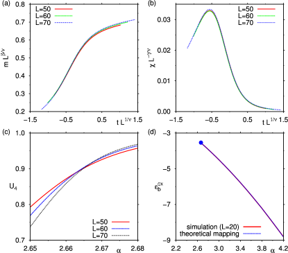
Figure 3: (Color online) Finite-size scaling results for the membrane without pinning sites. The scaling plots of the order parameter (a) and susceptibility (b) confirm 2D Ising universality, as indicated by the collapse of the data from different system sizes. The intersection of the Binder cumulant curves for different system sizes (c) yields an estimate of $\alpha^{\ast}$ consistent with the scaling plots. The variation of $\varepsilon_{\text{b}}^{\text{cx}}$ with $\alpha$ (d) conforms to the theoretical prediction, where the dot marks the critical point.

In Fig. 3(a), we show the scaling plot of the order parameter Newman and Barkema (1999), i.e., curves of $mL^{\beta/\nu}$ versus $tL^{1/\nu}$, $t=\alpha/\alpha^{\ast}-1$, using 2D Ising critical exponents $\beta=1/8$, $\nu=1$, and with $\alpha^{\ast}=2.665$ obtained by tuning until the curves for different $L$ collapsed (note: we use the “standard symbol” $\beta$ for the order parameter critical exponent, which is not to be confused with the inverse temperature). The fact that the data collapse confirms 2D Ising universality, and our estimate of $\alpha^{\ast}$ is in good agreement with Ref. Weikl et al., 2002. In Fig. 3(b), we show the corresponding scaling plot of the susceptibility, using the 2D Ising value $\gamma=7/4$, while for $\alpha^{\ast}$ the above estimate was used. A data collapse is again observed, providing further confirmation of 2D Ising universality. In Fig. 3(c), we plot the Binder cumulant $U_{4}$ versus $\alpha$. In agreement with a critical point, the curves for different $L$ intersect at $\alpha^{\ast}$.

IV.2.2 Symmetry line

In Fig. 3(d), the variation of $\varepsilon_{\text{b}}^{\text{cx}}$ with $\alpha$ as obtained in our simulations using Eq. (20) is shown. Coexistence of the bound and the unbound phases occurs along this symmetry line, $\varepsilon_{\text{b}}=\varepsilon_{\text{b}}^{\text{cx}}(\alpha)$, which implies that the Hamiltonian is invariant under “swapping” the two coexisting phases. For the discrete Hamiltonian Eq. (13) this corresponds to the operation

$$(\delta_{i},b_{i})\mapsto(-\delta_{i},1-b_{i}),$$ (21)

where $\delta_{i}\equiv h_{i}-\langle h\rangle$ is the height deviation at lattice site $i$ around the mean membrane height $\langle h\rangle$. A straightforward calculation shows that, in order for $\mathcal{H}_{N}$ to be invariant, we are left with the condition

$$(2\langle h\rangle+\alpha)\frac{1}{N}\sum_{i=1}^{N}\delta_{i}=(\alpha\langle h\rangle-\varepsilon_{\text{b}}^{\text{cx}})(1-2\phi).$$ (22)

Hence, the mean height along the symmetry line obeys $\langle h\rangle=-\alpha/2$. Comparing this result with an alternative calculation in appendix C we find that $\langle\phi\rangle=1/2$ along the symmetry line, as expected. Moreover, from the second condition we obtain the symmetry line: $\varepsilon_{\text{b}}^{\text{cx}}=-\alpha^{2}/2$. As Fig. 3(d) shows, the agreement with the simulation result is excellent.

In the effective model Eq. (5), spin-reversal symmetry corresponds to the operation $b_{i}\mapsto 1-b_{i}$. The symmetry line is now determined through

$$\mu_{0}^{\text{cx}}=-\frac{1}{2}\sum_{j\neq i}\varepsilon_{ij}=\varepsilon_{\text{b}}^{\text{cx}}+\varepsilon_{0}/2,$$ (23)

where the sum runs over all sites $j$ excluding $i$. Plugging in the definition Eq. (6) for the coupling energy $\varepsilon_{0}$, the binding energy at coexistence is $\varepsilon_{\text{b}}^{\text{cx}}=-c\alpha^{2}$ with $c=(\xi_{\perp}^{2}/2)(1+4\epsilon_{\text{A}}+4\epsilon_{\text{B}}+\dots)$. The prefactor $c$ apparently depends on the correlation length $\xi_{\parallel}$ determining the interaction range, but should nevertheless converge to $c=1/2$. We have checked for $\xi_{\parallel}=1$ that this is indeed the case [Fig. 3(d)].

At the coexistence binding energy, $\varepsilon_{\text{b}}^{\text{cx}}=-\alpha^{2}/2$, the order parameter probability $P(\phi)$ is symmetric about $\phi=1/2$ [Fig. 4(a)]. The latter reflects the spin-reversal symmetry of the Ising model, which persists in the membrane model as becomes evident from the theoretical mapping. We emphasize that this applies to the membrane without pinning sites: in the presence of pinning sites, spin-reversal symmetry is generally broken. Instead of using the density of closed bonds $\phi$ as the order parameter, we could also have used the membrane height per site $h=(1/L^{2})\sum_{i}h_{i}$ Weikl et al. (2002) since the latter is directly coupled to the density of closed bonds. This can also be seen in Fig. 4(c), where we show the same snapshot as in (b), but this time color-coded according to the membrane height. Furthermore, in a canonical (fixed $\phi$) simulation, and using the symmetry value $\phi=1/2$, the binding energy always assumes the coexistence value $\varepsilon_{\text{b}}^{\text{cx}}$ (for the Ising model with conserved order parameter Newman and Barkema (1999), the analogue of this condition is that, at zero magnetization, the external field is zero). In a grand-canonical simulation, i.e., where $\phi$ is allowed to fluctuate, and using the coexistence binding energy $\varepsilon_{\text{b}}^{\text{cx}}$, the probability distribution of the membrane height $P(h)$ will thus be symmetric about $h=-\alpha/2$.

IV.2.3 Line tension

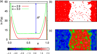
Figure 4: (Color online) (a) Free energy $\ln P(\phi)$ at coexistence for two values $\alpha\gg\alpha^{\ast}$ using a rectangular $50\times 100$ simulation lattice. The vertical double-arrow indicates the free energy cost $\Delta F$ of interface formation. Note the pronounced flat region between the peaks. (b) Snapshot of the membrane at $\phi=1/2$ and $\alpha=2.9$, where the dots indicate closed bonds. (c) The same snapshot, but color-coded according to the membrane height. The snapshots (b,c) clearly indicate that, in regions with a high density of closed bonds, the membrane is “pulled down”.

Next, we consider $\alpha\gg\alpha^{\ast}$, where the transition is strongly first-order. In Fig. 4(a), we show $\ln P(\phi)$ at coexistence for two values of $\alpha$, using a rectangular $50\times 100$ simulation box (note that $\ln P(\phi)$ may be regarded as minus the free energy of the system). We observe that $\ln P(\phi)$ is profoundly bimodal, which indicates two-phase coexistence. The left peak corresponds to the unbound phase (low density of closed bonds), the right peak to the bound phase (high density of closed bonds), while in the region “between the peaks” both phases appear simultaneously. The latter follows strikingly from snapshots, see Fig. 4(b), which was taken at $\phi=0.5$. For this value of $\phi$, the phases arrange in two slabs, with two interfaces perpendicular to the longest edge, as this minimizes the total length of the line interface (whose length then equals $L_{\rm tot}=2L_{\rm short}$, with $L_{\rm short}=50$ the shortest edge of the simulation box). Provided the interfaces do not interact, there is a region over which $\phi$ can be varied without any free energy cost. This, apparently, is the case here, as the distributions $\ln P(\phi)$ are essentially flat in their center regions. Following Binder Binder (1982), we may then relate the free energy barrier $\Delta F$, indicated in Fig. 4(a) for $\alpha=3.0$, to the line tension $\sigma=\Delta F/L_{\rm tot}$. Applying this equation to the distributions of Fig. 4(a), we obtain $\sigma\simeq 0.34\,(0.48)$ for $\alpha=2.9\,(3.0)$, in units of $k_{B}T$ per lattice spacing. As expected, $\sigma$ decreases upon lowering $\alpha$.

IV.2.4 Summary

For the membrane without pinning, our simulation results are thus fully consistent with the theoretical prediction that such a system should map onto the 2D Ising lattice gas. By means of finite-size scaling, 2D Ising critical exponents are confirmed, the quadratic variation of the coexistence binding energy with $\alpha$ is recovered, and we observe the analogue of spin-reversal symmetry. Furthermore, our estimate of $\alpha^{\ast}$ is in good agreement with Ref. Weikl et al., 2002, providing an important consistency check for the composite MC moves proposed in this work. Finally, for $\alpha\gg\alpha^{\ast}$, we observe a first-order phase transition between bound and unbound phases, with an associated coexistence region where macroscopic domain formation occurs.

IV.3 The pinned membrane

We now consider a membrane with a finite concentration of pinning sites $\rho>0$. We continue to use $\kappa=\gamma=1$ in Eq. (13), for which the case without pinning was just described (Section IV.2). In what follows, we restrict ourselves to $\rho\ll 1$, i.e., the limit of low pinning concentration. We believe this to be the biologically most relevant situation, as well as the physically most interesting one (in the opposite limit $\rho\to 1$, the pinning sites would completely freeze the membrane, thereby trivially preventing any membrane-mediated phenomena from taking place).

IV.3.1 Numerical evidence for random-field disorder

The key prediction of the theoretical mapping, Eq. (5), is that, in the presence of pinning sites, the chemical potential becomes a quenched random variable (i.e., dependent on the spatial location in the sample, but without any time dependence). We thus expect “special regions” in the membrane where bonds prefer to close, which are those regions where the local chemical potential excess is positive. To test whether such regions can be found, we perform canonical MC simulations at a fixed fraction of closed bonds $\phi=1/2$. For each lattice site $i$, we measure the thermally averaged bond occupation variable $\langle b_{i}\rangle$, and use these to compute the spatial fluctuation Fischer and Vink (2011); Fischer et al. (2012)

$$\chi_{S}^{2}=[\langle b\rangle^{2}]-[\langle b\rangle]^{2},\qquad[\langle b\rangle^{n}]=\frac{1}{N}\sum_{i=1}^{N}\langle b_{i}\rangle^{n},$$ (24)

where the sum is over all lattice sites. In the absence of spatial preference, $\langle b_{i}\rangle=1/2$ for all sites, implying that $\chi_{S}=0$. However, if sites in certain regions prefer closed bonds, then $\langle b_{i}\rangle$ will be distinctly different from $1/2$, and consequently $\chi_{S}>0$.

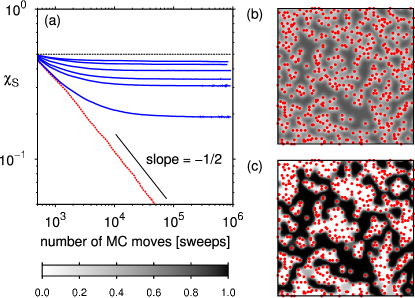
Figure 5: (Color online) (a) The “running average” of $\chi_{S}$, Eq. (24), which measures the spatial fluctuation in the thermally averaged bond occupation variables $\langle b_{i}\rangle$. The solid curves (blue) correspond to a pinned membrane for $\alpha=2.0,2.5,\alpha^{\ast},3.0,3.5,4.0$ (from bottom to top) where $\alpha^{\ast}$ is the critical point of the unpinned membrane. As $\alpha$ increases, $\chi_{S}\to 1/2$ (horizontal line). The dashed curve (red) shows $\chi_{S}$ for the membrane without pinning at $\alpha=2.5$, in which case $\chi_{S}$ decays to zero. (b,c) “Color-maps” of the thermally averaged bond occupation variables $\langle b_{i}\rangle$ for $\alpha=2.0$ (b), and $\alpha=4.0$ (c). In both cases, the same pinning configuration (red dots) is used. (All data in this figure refer to $L=100$; results for the pinned membrane use $\rho=0.05$ and $h_{\text{P}}=0$).

In Fig. 5(a), we show “running averages” of $\chi_{S}$ as a function of the number of MC moves $\tau$. For the unpinned membrane, $\chi_{S}$ decays to zero, since here there is no spatial preference. In the absence of spatial preference, $\chi_{S}$ reflects the statistical error of our simulation, and therefore decays $\propto\tau^{-1/2}$. In contrast, for the membrane with pinning sites, $\chi_{S}$ saturates to a finite plateau value. Note that this happens for all values of $\alpha$ considered, including those values below the critical point $\alpha^{\ast}$ of the unpinned membrane. By increasing $\alpha$, the plateau value increases, which means that the spatial preference becomes stronger. When $\alpha$ is small, thermal fluctuations still permit “excursions” of bonds into regions where the local chemical potential is unfavorable. In this case, $\langle b_{i}\rangle$ does not deviate much from $1/2$. As $\alpha$ increases, these thermal fluctuations are “frozen out”. In the limit $\alpha\to\infty$, the bond occupation variables are set by the groundstate of Eq. (13) (that is: for a given configuration of pinning sites, the variables $b_{i}$ are determined by energy minimization). In this limit, $\langle b_{i}\rangle$ is either 0 or 1, and the fluctuation $\chi_{S}=1/2$. As can be seen in Fig. 5(a), this limiting value is indeed approached as $\alpha$ increases.

However, already for $\alpha$ much smaller, the groundstate reveals itself. To demonstrate this, we show “color-maps” of the thermally averaged values $\langle b_{i}\rangle$ Fischer and Vink (2011); Fischer et al. (2012), for two values of $\alpha$, but using the same configuration of pinning sites with $h_{\text{P}}=0$ [Fig. 5(b,c)]. Clearly visible is that the adhesion domains (dark regions) prefer the same locations for both values of $\alpha$. The only difference is that, with increasing $\alpha$, the preference becomes stronger. The structure of Fig. 5(c) is already close to the groundstate, since the majority of $\langle b_{i}\rangle$ are already close to either 0 or 1. But also for the smaller value of $\alpha$, the groundstate is visible, albeit somewhat “blurred”. Note that $\alpha$ in Fig. 5(b) is considerably below $\alpha^{\ast}$ of the unpinned membrane, i.e., the presence of the groundstate persists deep into the high-temperature region.

Our finding that, in the presence of pinning sites, $\langle b_{i}\rangle$ generally deviates from $1/2$ may be conceived as a local chemical potential excess (field) at site $i$ given by

$$\Delta\mu_{i}=\ln\frac{\langle b_{i}\rangle}{1-\langle b_{i}\rangle},$$ (25)

where the canonical ensemble with $\phi=1/2$ is assumed. Furthermore, the “color-maps” of Fig. 5(b,c) suggest that $\Delta\mu_{i}$ is a spatially random variable. Since the chemical potential is isomorphic to an external field in the Ising model, this indeed corresponds to random-field disorder. Consequently, the pinned membrane belongs to the universality class of the two-dimensional random-field Ising model. This implies that the “freezing out” of the thermal fluctuations with increasing $\alpha$ in Fig. 5 is a gradual process, i.e., there is no phase transition associated with it (and nothing special happens at the critical point $\alpha^{\ast}$ of unpinned membrane). As is well known, the random-field Ising model in $d=2$ dimensions does not support any phase transition Nattermann (1998).

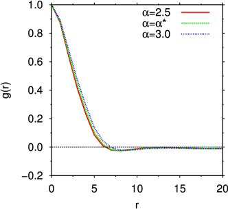
Figure 6: (Color online) The (normalized) correlation function $g(r)$ of the local chemical potential excess $\Delta\mu_{i}$, for several values of $\alpha$. The correlations quickly decay to zero, which confirms the prediction of the mapping that $\Delta\mu_{i}$ is a spatially random variable (results refer to the pinned membrane with $\rho=0.05$, $h_{\text{P}}=0$, and $L=100$).

To confirm that $\Delta\mu_{i}$ truly is a spatially random variable, we have measured the (circularly averaged) correlation function $g(r)\propto[\Delta\mu_{i}\Delta\mu_{j}]^{\prime}$, where $[\cdot]^{\prime}$ denotes a spatial average over pairs of sites $(i,j)$ a distance $r$ apart. As can be seen in Fig. 6, $g(r)$ quickly decays to zero. For randomly distributed pinning sites, the spatial correlations in the local chemical potential excess are thus short-ranged. Note also that $g(r)$ depends only weakly on $\alpha$. This is consistent with the “color-maps” of Fig. 5(b,c), whose overall topology (i.e., the shape of the regions) is also remarkably insensitive to $\alpha$. The insensitivity to $\alpha$ shows that the sign of the local chemical potential excess in Eq. (25) is determined exclusively by the properties of the membrane and the pinning sites (most notably the positions of the latter, and the pinning height $h_{\text{P}}$). The picture that one should have in mind, therefore, is that of ligand-receptor bonds “diffusing” through a chemical potential landscape, but the landscape itself is quenched, i.e., the bonds do not modify nor shape it. Incidentally, for $h_{\text{P}}=0$, Fig. 5(b,c) shows that the local chemical potential excess is such that the pinning sites “repel” closed bonds. By using a sufficiently negative pinning height, the reverse situation can be realized also.

IV.3.2 Adhesion domains are finite: Imry-Ma argument

For the pinned membrane, Figs. 5 and 6 clearly show that the local chemical potential excess is a quenched random variable, thereby confirming the theoretical prediction. This rigorously rules out the formation of large (macroscopic) adhesion domains, by virtue of the Imry-Ma argument Imry and Ma (1975); Imbrie (1984); Bricmont and Kupiainen (1987); Aizenman and Wehr (1989). To see this, consider a cluster of closed bonds of linear size $l$, thereby containing $\propto l^{d}$ bonds, and imagine to insert the cluster at some location in the sample. The average chemical potential excess (per site) over the cluster is zero, but with fluctuations that decay conform the central limit theorem

$$\frac{1}{l^{d}}\sum_{i\in\rm cluster}\Delta\mu_{i}=0\pm C/l^{d/2},$$ (26)

with $\Delta\mu_{i}$ given by Eq. (25), and $C$ a constant. Hence, there exist “preferred regions” where the cost of insertion is reduced by an amount $\propto l^{d/2}$. In $d=2$ dimensions (but not in $d=3$ Nattermann (1998); Vink et al. (2010)), this is sufficient to compensate the line tension, which scales $\sim l^{d-1}$. In the presence of pinning sites, adhesion domains thus no longer strive to minimize the length of their line interface. Instead, they seek out those regions in the sample where the local chemical potential excess is most favorable, precisely what is observed in Fig. 5(b,c). We thus obtain a stable multi-domain structure. Note the sharp contrast to the case without pinning, where adhesion domains do minimize their interface, thereby growing macroscopically large [Fig. 4].

IV.3.3 Domain size statistics

Having argued that adhesion domains in the presence of pinning sites remain finite, we now present a more quantitative analysis of their size. As the domain structure is essentially fixed by the pinning sites, and much less by thermal effects, we restrict ourselves to $\alpha=3.5$, and vary only (i) the pinning concentration $\rho$, and (ii) the lateral correlation length $\xi_{\parallel}$ of the membrane fluctuations. The simulations in this section are again performed in the canonical ensemble ($\phi=1/2$), and pinning height $h_{\text{P}}=0$ (pinning sites thus “repel” closed bonds). The remaining fixed parameters are $\gamma=1$ for the non-specific potential, and system size $L=100$.

For a given sample $i=1,\ldots,K$ of pinning sites, we generate a series $t=1,\ldots,T$ of equilibrated snapshots. For each snapshot, we compute the typical domain size $R_{t,i}=2\pi\int S_{t,i}(k)\,dk/\int kS_{t,i}(k)\,dk$ Newman and Barkema (1999), where $S_{t,i}(k)$ is the (circularly averaged) static structure factor; disorder $[\cdot]$ and thermal $\langle\cdot\rangle$ averages are then computed as

$$[\langle R^{n}\rangle^{m}]=\frac{1}{K}\sum_{i=1}^{K}\left(\frac{1}{T}\sum_{t=1}^{T}R_{t,i}^{n}\right)^{m}.$$ (27)

We will primarily be concerned with the average domain size $[\langle R\rangle]$, the thermal fluctuations $\chi_{T}^{2}\equiv\langle R^{2}\rangle-\langle R\rangle^{2}$, and the disorder fluctuations $\chi_{D}^{2}\equiv[\langle R\rangle^{2}]-[\langle R\rangle]^{2}$.

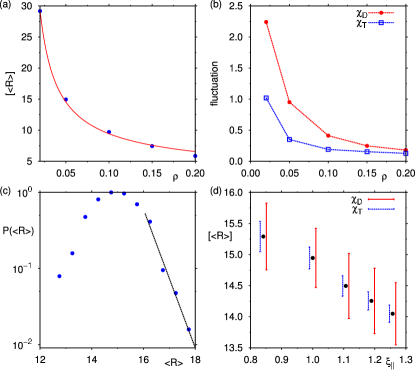
Figure 7: (Color online) (a) Average domain size $[\langle R\rangle]$ as function of pinning density $\rho$ (symbols are simulation data; the curve is a fit to Eq. (28)). (b) The disorder fluctuation $\chi_{D}$ and the thermal fluctuation $\chi_{T}$ in the domain size as function of $\rho$. (c) Distribution of the thermally averaged domain size between samples for $\rho=0.05$. Note the logarithmic vertical scale. The dashed line shows the result of an exponential fit (see details in text). (d) Variation of the typical domain size $[\langle R\rangle]$ with the lateral correlation length $\xi_{\parallel}$ (dots). Also shown for each measurement are the magnitudes of the disorder $\chi_{D}$ and thermal fluctuations $\chi_{T}$. (Note: All averages in this figure were computed using Eq. (27) with $T\sim 500$, $K=20$ (a,b,d), and $K=500$ (c). The data in (a-c) were obtained for $\kappa=1$, while in (d) $\kappa$ was varied.)

In Fig. 7(a), we plot the average domain size $[\langle R\rangle]$ as function of the pinning concentration $\rho$. As might be expected, the domain size decreases with increasing concentration. Following theoretical predictions for the random-field Ising model Binder (1983); Grinstein and Ma (1983); Seppälä et al. (1998), we anticipate that

$$\ln\,[\langle R\rangle]\propto\rho^{-p}\quad,$$ (28)

with exponent $p>0$, whereby we assume that $[\langle R\rangle]$ is the analogue of the “break-up” length. For bimodal and Gaussian random-fields $p=2$, but since it is a priori unclear how pinning sites compare to such fields, we leave $p$ as a free parameter. The curve in Fig. 7(a) shows the corresponding fit of Eq. (28) to our data, where $p\simeq 0.25$ was used, and the agreement is quite reasonable.

Next, we consider the magnitude of the thermal $\chi_{T}$ and disorder fluctuations $\chi_{D}$ [Fig. 7(b)]. As $\rho$ increases, the fluctuations become smaller, but we always find that $\chi_{D}>\chi_{T}$. The disorder fluctuations thus dominate, as we had already announced previously. In Fig. 7(c), we plot the distribution $P(\langle R\rangle)$ of the thermally averaged domain size $\langle R\rangle$ between samples for $\rho=0.05$ (the width of this distribution thus reflects the disorder fluctuation $\chi_{D}$). Experiments have indicated that the tail of the distribution is exponential Gov (2006). The dashed line in Fig. 7(c) shows a fit to the tail of the simulated distribution using an exponential function of the form $P(x)\propto e^{-bx}$. The fit captures the data rather well, where $b\simeq 2.1$ was used.

Last but not least, we show in Fig. 7(d) the variation of the average domain size $[\langle R\rangle]$ with the lateral correlation length $\xi_{\parallel}$. As $\xi_{\parallel}$ increases, there is a mild decrease of the domain size. However, on the scale of the (dominating) disorder fluctuations, the effect may be difficult to observe in experiments.

IV.3.4 The case of “neutral” pinning sites

Figure 8: (Color online) Simulation results for the pinned membrane using pinning height $h_{\text{P}}=h_{\text{P}}^{\ast}=-\alpha/2$. In this case, there is no random-field effect. (a) The “running average” of the spatial fluctuation $\chi_{S}$. Clearly visible is that $\chi_{S}\to 0$. (b) The “running average” of the chemical potential $\mu$, which approaches $\varepsilon_{\text{b}}^{\text{cx}}$ (horizontal line). All data refer to $\rho=0.05,\alpha=2.0,L=40$. In each plot, results from five independent simulation runs are shown.

As can be seen in Fig. 5(b,c), for $h_{\text{P}}=0$ the pinning sites “repel” closed bonds. When the pinning height is sufficiently negative, the reverse situation is obtained and pinning sites attract closed bonds (we have checked this case for $h_{\text{P}}=-\alpha$). Therefore, it is plausible that for some intermediate height $h_{\text{P}}^{\ast}$ the pinning sites become neutral. This special height is given by the symmetry height of the unpinned membrane: $h_{\text{P}}^{\ast}=-\alpha/2$ (Section IV.2.2). Consequently, when $h_{\text{P}}=h_{\text{P}}^{\ast}$, we no longer expect the local chemical potential excess to be a quenched random variable, but rather $\Delta\mu_{i}=0$ for all sites.

To test this assertion, we performed a canonical simulation ($\phi=1/2$) using pinning concentration $\rho=0.05$, pinning height $h_{\text{P}}=h_{\text{P}}^{\ast}$, and $\alpha=2.0$. In Fig. 8(a), we plot the “running average” of the spatial fluctuation $\chi_{S}$ in the thermally averaged bond occupation variables (Eq. (24)). The figure strikingly shows $\chi_{S}\to 0$, which confirms that the local chemical potential excess has indeed vanished. As for the unpinned membrane, $\chi_{S}$ now reflects the statistical error of our MC simulation, and therefore decays $\propto\tau^{-1/2}$, $\tau$ being the number of MC moves. This result is to be contrasted with Fig. 5(a), where $\chi_{S}$ for the pinned membrane converged to a finite value. Hence, even though the pinning concentration is the same in both cases, choosing $h_{\text{P}}=h_{\text{P}}^{\ast}$ completely destroys the random-field effect. In Fig. 8(b), we show the “running average” of the chemical potential obtained via Widom insertion Widom (1963); Frenkel and Smit (2001). Interestingly, $\mu$ converges exactly onto $\varepsilon_{\text{b}}^{\text{cx}}=-\alpha^{2}/2$ of the unpinned membrane. Apparently, for neutral pinning sites, the symmetry line of the unpinned membrane is restored.

At $h_{\text{P}}=h_{\text{P}}^{\ast}$, the Imry-Ma argument thus no longer applies. We therefore expect a critical point again, at $\alpha=\alpha^{\prime}$, and macroscopic adhesion domains for $\alpha>\alpha^{\prime}$. The value of $\alpha^{\prime}$ should increase with $\rho$, and $\lim_{\rho\to 0}\alpha^{\prime}=\alpha^{\ast}$ of the unpinned membrane. The quenched disorder induced by neutral pinning sites is of the dilution type. The diluted Ising model is similar to the standard Ising model, but with a (small) fraction of randomly selected sites removed from the lattice Mazzeo and Kühn (1999). Note that this type of quenched disorder does not break spin reversal symmetry, consistent with our observation that $\mu\to\varepsilon_{\text{b}}^{\text{cx}}$ [Fig. 8(b)].

In realistic situations, we do not expect the pinning sites to be neutral, nor that the pinning height is the same for all pinning sites (as assumed in the present study). In all these cases, it is the random-field scenario that applies. Nevertheless, for our fundamental understanding we felt inclined to discuss the neutral case also.

V Summary and Conclusions

We have studied a minimal model Weikl et al. (2002); Weikl and Lipowsky (2007) describing the specific adhesion of a cell (or biomimetic vesicle) to another cell, the extracellular matrix, or a substrate. The model incorporates the arguably most important mechanism: the coupling of thermal fluctuations of the cell membrane to the state of the receptor-ligand pairs responsible for the cell attachment. The latter are effectively described as either open or closed bonds. Integrating out the membrane fluctuations this model can be mapped exactly onto the two-dimensional lattice gas (or Ising model). This mapping confirms previous numerical evidence of a phase separation Weikl et al. (2002) between an unbound and a bound state. For fixed concentration of mobile bonds this scenario implies the formation of a single macroscopic domain of bonds. Moreover, we have exactly determined the critical point, and we have demonstrated numerically that the full model indeed belongs to the Ising universality class as anticipated from the theoretical mapping.

A striking observation in experiments is the absence of a single large domain. Rather, adhesion domains of finite size form. This observation is often explained as either caused by active processes, or the “corralling” of adhesion proteins in compartments Kusumi et al. (2005). This putative hindrance of protein diffusion is a purely dynamical approach, which does not alter equilibrium properties. Quite in contrast, here we have demonstrated that already in equilibrium finite sized adhesion domains are implied in a wide variety of contexts if one takes into account “pinning sites” that locally suppress membrane height fluctuations. These pinning sites model perturbations that necessarily occur in vivo due to the crowded, highly non-ideal composition of cell membranes and the anchoring of the cytoskeleton to the ECM or other cells.

We have presented both analytical calculations and numerical evidence that the presence of pinning sites corresponds to quenched disorder which, in the language of the Ising model, induces a random field that prevents macroscopic domain formation in two dimensions Imry and Ma (1975); Imbrie (1984); Bricmont and Kupiainen (1987); Aizenman and Wehr (1989). This is in sharp contrast to the type of quenched disorder where the positions of ligand-receptor bonds are random. The latter constitutes a marginal perturbation Lipowsky (1996) and does not fundamentally alter the scenario of Fig. 4, i.e., macroscopic domain formation above some critical $\alpha$. In contrast, random-field disorder is a relevant perturbation. It requires that the disorder couples linearly to the order parameter. We have demonstrated here that this condition is typically fulfilled for membrane adhesion, where membrane height pinning (disorder) couples to bond formation (order parameter $\phi$). Hence, the fundamentals of statistical physics can be used to explain adhesion domains of finite size in equilibrium.

Appendix A Height correlations

Using periodic boundaries the separation profile $h(\mathbf{r})$ is expanded into Fourier modes through

$$h(\mathbf{r})=\sum_{\mathbf{q}}h_{\mathbf{q}}e^{-\text{i}\mathbf{q}\cdot\mathbf{r}},\qquad h_{\mathbf{q}}=\frac{1}{A}\int_{A}\mathrm{d}^{2}\mathbf{r}\;h(\mathbf{r})e^{\text{i}\mathbf{q}\cdot\mathbf{r}}$$

with $h_{\mathbf{q}}=h^{\prime}_{\mathbf{q}}+\text{i}h^{\prime\prime}_{\mathbf{q}}$. Since the separation field is real

$$h(\mathbf{r})=h_{0}+2\sum_{\mathbf{q}\in\mathcal{Q}}[h^{\prime}_{\mathbf{q}}\cos(\mathbf{q}\cdot\mathbf{r})+h^{\prime\prime}_{\mathbf{q}}\sin(\mathbf{q}\cdot\mathbf{r})],$$

where the set $\mathcal{Q}$ contains the independent wave vectors excluding $q=0$.

For a free membrane in the absence of both bonds and pinning sites the Hamiltonian Eq. (1) in Fourier space reads

$$\beta\mathcal{H}_{0}=\frac{1}{2}\gamma_{0}h_{0}^{2}+\frac{1}{2}\sum_{\mathbf{q}\in\mathcal{Q}}\gamma_{q}(h_{\mathbf{q}}^{\prime 2}+h_{\mathbf{q}}^{\prime\prime 2})$$

with $\gamma_{0}\equiv\beta A\gamma$ and $\gamma_{q}\equiv 2\gamma_{0}[1+(q\xi_{\parallel})^{4}]$. Hence, the mean height is $\langle h(\mathbf{r})\rangle_{0}=0$ and the height correlations read

$$m(|\mathbf{r}-\mathbf{r}^{\prime}|)\equiv\langle h(\mathbf{r})h(\mathbf{r}^{\prime})\rangle_{0}=\frac{1}{\gamma_{0}}+4\sum_{\mathbf{q}\in\mathcal{Q}}\frac{\cos\mathbf{q}\cdot(\mathbf{r}-\mathbf{r}^{\prime})}{\gamma_{q}}.$$

The height correlations between two points on the membrane decay on the length scale $\xi_{\parallel}$. For large separations they reach $m(r\rightarrow\infty)=\langle h_{0}^{2}\rangle_{0}=1/\gamma_{0}$ due to the zero mode fluctuations. For large $A$ we can neglect this contribution. Replacing the sum over discrete wave vectors by an integral we then obtain

$$m(r)\approx\frac{\xi_{\parallel}^{4}}{2\pi\beta\kappa}\int_{0}^{\infty}\mathrm{d}q\;\frac{qJ_{0}(qr)}{1+(q\xi_{\parallel})^{4}},$$

where $J_{0}$ is the zero-order Bessel function of the first kind. Performing the final integration leads to Eq. (2) for the height correlations of a free membrane.

Appendix B Effective free energy

The full partition sum of the system reads

$$\mathcal{Z}=\sum_{\{b_{i}\}}\int[\mathrm{d}h(\mathbf{r})]\;\int\mathrm{d}h_{1}\cdots\mathrm{d}h_{N}\;e^{-\beta\mathcal{H}_{N}}\\ \times\prod_{i=1}^{N}\delta(h(\mathbf{r}_{i})-h_{i})\prod_{k=N+1}^{M}\ell\delta(h(\mathbf{r}_{k})-h_{\text{P}}),$$ (29)

where the Hamiltonian $\mathcal{H}_{N}$ is given in Eq. (3). The $M=N+n$ total constraints due to the $N$ bonds and the presence of $n$ pinning sites are represented through $\delta$-functions, where $\ell$ is a microscopic length. We normalize the functional measure such that $\mathcal{Z}=1$ for a free membrane.

As usual, we represent the $\delta$-functions as integrals

$$\delta(h(\mathbf{r}_{i})-h_{i})=\frac{1}{2\pi}\int\mathrm{d}\lambda_{i}\;e^{\text{i}\lambda_{i}[h(\mathbf{r}_{i})-h_{i}]},$$

where we complement $h_{i}=h_{\text{P}}$ for $i>N$. This allows us to write the partition sum Eq. (29) involving a single exponential

$$\mathcal{Z}=\sum_{\{b_{i}\}}\int[\mathrm{d}h(\mathbf{r})]\;\frac{\ell^{n}}{(2\pi)^{M}}\int\mathrm{d}\lambda_{1}\cdots\mathrm{d}\lambda_{M}\;\int\mathrm{d}h_{1}\cdots\mathrm{d}h_{N}\;\exp\left\{-\beta\mathcal{H}_{0}+c_{0}h_{0}+\sum_{\mathbf{q}\in\mathcal{Q}}(c_{\mathbf{q}}^{\prime}h_{\mathbf{q}}^{\prime}+c_{\mathbf{q}}^{\prime\prime}h_{\mathbf{q}}^{\prime\prime})-\text{i}\sum_{i=1}^{M}\lambda_{i}h_{i}+\beta\varepsilon_{\text{b}}\sum_{i=1}^{N}b_{i}\right\}$$

with coefficients

$$c_{0}\equiv\text{i}\sum_{i=1}^{M}\lambda_{i}-\beta\alpha\sum_{i=1}^{N}b_{i},$$

$$c_{\mathbf{q}}^{\prime}\equiv 2\text{i}\sum_{i=1}^{M}\lambda_{i}\cos\mathbf{q}\cdot\mathbf{r}_{i}-2\beta\alpha\sum_{i=1}^{N}b_{i}\cos\mathbf{q}\cdot\mathbf{r}_{i},$$

$$c_{\mathbf{q}}^{\prime\prime}\equiv 2\text{i}\sum_{i=1}^{M}\lambda_{i}\sin\mathbf{q}\cdot\mathbf{r}_{i}-2\beta\alpha\sum_{i=1}^{N}b_{i}\sin\mathbf{q}\cdot\mathbf{r}_{i}.$$

Note that the first sum runs over all sites whereas the second sum only includes the sites where bonds are present. Performing the Gaussian integrations over the height modes $\{h_{\mathbf{q}}\}$ and the auxiliary variables $\{\lambda_{i}\}$ we obtain

$$\mathcal{Z}=\frac{\ell^{n}}{(2\pi)^{M/2}}\sqrt{\det\mathsf{m}^{-1}}\sum_{\{b_{i}\}}\int\mathrm{d}h_{1}\cdots\mathrm{d}h_{N}\;\\ \times\exp\left\{-\frac{1}{2}\sum_{ij}^{M}(\mathsf{m}^{-1})_{ij}h_{j}h_{j}-\beta\sum_{i=1}^{N}b_{i}[\alpha h_{i}-\varepsilon_{\text{b}}]\right\}.$$ (30)

The prefactor is independent of the state of the bonds. While in principle it depends on the quenched disorder of the pinning sites it does not contribute to thermal averages. Setting $h_{\text{P}}=0$ the terms with indices $i>N$ corresponding to the pinning sites drop out of the sum and we obtain Eq. (4).

Appendix C Mean height

The derivation presented in the previous section is easily modified to calculate a generating function, from which arbitrary moments can be obtained. For example, replacing $c_{0}\rightarrow c_{0}+\lambda$ we obtain the generating function $\mathcal{Z}(\lambda)$ from which the mean height follows as

$$\langle h_{0}\rangle=\left.\frac{\partial\ln\mathcal{Z}(\lambda)}{\partial\lambda}\right|_{\lambda=0}.$$ (31)

Repeating the calculation for $n=0$ we obtain

$$\langle h_{0}\rangle=-\frac{\alpha N}{\gamma A}\langle\phi\rangle.$$ (32)

References

- Geiger et al. (2001) B. Geiger, A. Bershadsky, R. Pankov, and K. M. Yamada, Nat. Rev. Mol. Cell Biol. 2, 793 (2001).
- Parsons et al. (2010) J. T. Parsons, A. R. Horwitz, and M. A. Schwartz, Nat. Rev. Mol. Cell Biol. 11, 633 (2010).
- Nicolas et al. (2004) A. Nicolas, B. Geiger, and S. A. Safran, Proc. Natl. Acad. Sci. U.S.A. 101, 12520 (2004).
- Gov (2006) N. S. Gov, Biophys. J. 91, 2844 (2006).
- Bell (1978) G. I. Bell, Science 200, 618 (1978).
- Weikl et al. (2002) T. Weikl, D. Andelman, S. Komura, and R. Lipowsky, Eur. Phys. J. E 8, 59 (2002).
- Krobath et al. (2007) H. Krobath, G. J. Schütz, R. Lipowsky, and T. R. Weikl, EPL 78, 38003 (2007).
- Speck et al. (2010) T. Speck, E. Reister, and U. Seifert, Phys. Rev. E 82, 021923 (2010).
- Weil and Farago (2010) N. Weil and O. Farago, Eur. Phys. J. E 33, 81 (2010).
- Farago (2011) O. Farago, Advances in Planar Lipid Bilayers and Liposomes (Elsevier, 2011), vol. 14, chap. 5, pp. 129–155, ISBN 9780123877208.
- Lipowsky (1996) R. Lipowsky, Phys. Rev. Lett. 77, 1652 (1996).
- Zhang and Wang (2008) C.-Z. Zhang and Z.-G. Wang, Phys. Rev. E 77, 021906 (2008).
- Atilgan and Ovryn (2009) E. Atilgan and B. Ovryn, Biophys. J. 96, 3555 (2009).
- Tanaka and Sackmann (2005) M. Tanaka and E. Sackmann, Nature 437, 656 (2005).
- Mossman and Groves (2007) K. Mossman and J. T. Groves, Chem. Soc. Rev. 36, 46 (2007).
- Bruinsma et al. (2000) R. Bruinsma, A. Behrisch, and E. Sackmann, Phys. Rev. E 61, 4253 (2000).
- Cuvelier and Nassoy (2004) D. Cuvelier and P. Nassoy, Phys. Rev. Lett. 93, 228101 (2004).
- Reister-Gottfried et al. (2008) E. Reister-Gottfried, K. Sengupta, B. Lorz, E. Sackmann, U. Seifert, and A.-S. Smith, Phys. Rev. Lett. 101, 208103 (2008).
- Limozin and Sengupta (2009) L. Limozin and K. Sengupta, ChemPhysChem 10, 2752 (2009).
- Smith and Sackmann (2009) A.-S. Smith and E. Sackmann, ChemPhysChem 10, 66 (2009).
- Kusumi et al. (2005) A. Kusumi, C. Nakada, K. Ritchie, K. Murase, K. Suzuki, H. Murakoshi, R. S. Kasai, J. Kondo, and T. Fujiwara, Annu. Rev. Biophys. Biomol. Struct 34, 351 (2005).
- Imry and Ma (1975) Y. Imry and S.-k. Ma, Phys. Rev. Lett. 35, 1399 (1975).
- Imbrie (1984) J. Z. Imbrie, Phys. Rev. Lett. 53, 1747 (1984).
- Bricmont and Kupiainen (1987) J. Bricmont and A. Kupiainen, Phys. Rev. Lett. 59, 1829 (1987).
- Aizenman and Wehr (1989) M. Aizenman and J. Wehr, Phys. Rev. Lett. 62, 2503 (1989).
- Weikl and Lipowsky (2007) T. Weikl and R. Lipowsky, Advances in Planar Lipid Bilayers and Liposomes (Elsevier, 2007), vol. 5, chap. 4, pp. 64–127.
- Helfrich (1978) W. Helfrich, Z. Naturforsch. 33a, 305 (1978).
- Li and Kardar (1991) H. Li and M. Kardar, Phys. Rev. Lett. 67, 3275 (1991).
- Virnau and Müller (2004) P. Virnau and M. Müller, J. Chem. Phys. 120, 10925 (2004).
- Ferrenberg and Swendsen (1988) A. M. Ferrenberg and R. H. Swendsen, Phys. Rev. Lett. 61, 2635 (1988).
- Fischer and Vink (2011) T. Fischer and R. L. C. Vink, J. Chem. Phys. 134, 055106 (2011).
- Newman and Barkema (1999) M. E. J. Newman and G. T. Barkema, Monte Carlo Methods in Statistical Physics (Clarendon Press, Oxford, 1999).
- Binder (1982) K. Binder, Phys. Rev. A 25, 1699 (1982).
- Fischer et al. (2012) T. Fischer, H. Jelger Risselada, and R. L. C. Vink, Phys. Chem. Chem. Phys. (2012).
- Nattermann (1998) T. Nattermann, in Spin Glasses and Random Fields, edited by A. P. Young (World Scientific, Singapore, 1998), p. 277.
- Vink et al. (2010) R. L. C. Vink, T. Fischer, and K. Binder, Phys. Rev. E 82, 051134 (2010).
- Binder (1983) K. Binder, Z. Phys. B 50, 343 (1983).
- Grinstein and Ma (1983) G. Grinstein and S. K. Ma, Phys. Rev. B 28, 2588 (1983).
- Seppälä et al. (1998) E. T. Seppälä, V. Petäjä, and M. J. Alava, Phys. Rev. E 58, R5217 (1998).
- Widom (1963) B. Widom, J. Chem. Phys. 39, 2808 (1963).
- Frenkel and Smit (2001) D. Frenkel and B. Smit, Understanding Molecular Simulation (Academic Press, San Diego, 2001).
- Mazzeo and Kühn (1999) G. Mazzeo and R. Kühn, Phys. Rev. E 60, 3823 (1999).