Statistics of circular interface fluctuations
in an off-lattice Eden model

Abstract

Scale-invariant fluctuations of growing interfaces are studied for circular clusters of an off-lattice variant of the Eden model, which belongs to the $(1+1)$-dimensional Kardar-Parisi-Zhang (KPZ) universality class. Statistical properties of the height (radius) fluctuations are numerically determined and compared with the recent theoretical developments as well as the author’s experimental result on growing interfaces in turbulent liquid crystal [K. A. Takeuchi and M. Sano, arXiv:1203.2530]. We focus in particular on analytically unsolved properties such as the temporal correlation function and the persistence probability in space and time. Good agreement with the experiment is found in characteristic quantities for them, which implies that the geometry-dependent universality of the KPZ class holds here as well, but otherwise a few dissimilarities are also found. Finite-time corrections in the cumulants of the distribution are also studied and shown to decay, for the mean, as $t^{-2/3}$ within the time window of the simulations, instead of $t^{-1/3}$ which arises as the typical leading term in the previously known cases.

1 Introduction

Growing interfaces driven by local stochastic interactions constitute a prototypical example where scale invariance leads to universality even in systems far from equilibrium [1]. In their seminal work [2], Kardar, Parisi, and Zhang (KPZ) proposed a continuum equation for describing such growing interfaces, which reads

$$\frac{\partial}{\partial t}h(x,t)=\nu\nabla^{2}h+\frac{\lambda}{2}(\nabla h)^{2}+\xi(x,t)$$ (1)

with the local height $h(x,t)$ of the interfaces and the white Gaussian noise $\langle\xi(x,t)\rangle=0$ and $\langle\xi(x,t)\xi(x^{\prime},t^{\prime})\rangle=D\delta(x-x^{\prime})\delta(t-t^{\prime})$. They derived a set of characteristic exponents $\alpha=1/2$, $\beta=1/3$ and $z\equiv\alpha/\beta=3/2$ that describe scale-invariant fluctuations of the interfaces in $1+1$ dimensions, in agreement with the earlier theoretical studies on related problems [3, 4]. These exponents are universal as widely confirmed by theoretical and numerical work [1] as well as by a few experiments (see [5, 6, 7] and references therein), constituting the KPZ universality class. Recently, studies in this context entered an unprecedented phase, when Johansson rigorously derived the asymptotic distribution function for a model in the KPZ class [8] on tha basis of related combinatorial problems [9]; this spearheaded remarkable theoretical achievements marked in the last decade (for recent reviews, see [10, 11, 12]). Their main conclusions are twofold: (i) The distribution function and the spatial correlation function were obtained analytically for a few solvable models, including the KPZ equation [13, 14, 15, 16, 17, 18, 19], and revealed nontrivial connection to random matrix theory. (ii) These are expected to be universal, but nevertheless depend on the global shape of the interfaces, e.g., whether they are curved or flat, as first pointed out by Prähofer and Spohn [20]. In particular, the asymptotic distribution function for the curved interfaces is given by the largest-eigenvalue distribution of large random matrices in Gaussian unitary ensemble (GUE) [8, 20], called the GUE Tracy-Widom distribution [21], and for the flat interfaces by the corresponding distribution for Gaussian orthogonal ensemble (GOE) [20].

This detailed yet geometry-dependent universality of the KPZ class was recently underpinned by an experiment on growing interfaces of topological-defect turbulence in nematic liquid crystal, in which the author and his coworker identified the analytically obtained distribution functions and the spatial correlation functions for both circular and flat interfaces [5, 6, 7]. In [7] they further advanced their analyses to study statistical properties that remain analytically unsolved even for the solvable models, in particular those related to the temporal correlation of the interface fluctuations. This revealed that the difference between the circular and flat interfaces is not restricted to the distribution and spatial correlation functions, but actually arises in many other quantities as well, sometimes even with qualitative differences, as summarized in table 1 of [7]. These quantities — specifically, the temporal correlation function and the temporal and spatial persistence probabilities — are expected to be universal in the asymptotic limit when appropriately rescaled.

Here, as an approach complementary to the experiment, the author performs the same analyses for a numerical model, namely an off-lattice variant of the Eden model [22, 1] introduced in the present paper, and provides a numerical case study on the universality in those unsolved quantities. Focus in the present study is set on the circular interfaces, which are numerically much less studied than the flat case and are also more delicate: because the circumference, or the system size of the interface, is by construction finite at finite times and grows with time, the ensemble and the spatial averages lead to different results when they are used to define the statistical quantities [7]. Using the spatial average instead of the ensemble one yields false estimates even for the growth exponent $\beta$ [7]. Since this point has not been explicitly recognized in past studies, it is important to provide a set of reliable numerical estimates for the circular interfaces of a numerical model — this is the aim of the present paper.

2 Model

Only few numerical models are known to produce circular interfaces, most of which are variants of the Eden model. The Eden model was originally defined on a lattice. Starting with a seed particle at the origin, at each time step one adds a new particle on a randomly chosen site on the perimeter of the cluster [22, 1]. This however turned out to induce anisotropy due to the lattice structure [1, 23] unless a specific growth rule is introduced, such as the growth probability dependent on the number of the occupied nearest-neighbors [24, 25]. Off-lattice versions of the Eden model have therefore been considered occasionally in the literature [26, 27, 28, 25], but in most cases time $t$ is measured by the global radius $\langle h\rangle$ of the radial cluster, which is not correct at finite times because the two quantities are in general connected by $\mathrm{d}\langle h\rangle/\mathrm{d}t\simeq v_{\infty}+c_{v}t^{-2/3}$ [29, 5, 6, 7]. To resolve these problems, as well as to study a numerical model that the author considers better corresponds to a coarse-grained picture for the experimentally investigated growth of the liquid-crystal turbulence [5, 6, 7], a new variant of the off-lattice Eden model is introduced and studied in the present paper.

The model is defined as follows. First, place a round particle of unit diameter at the origin of two-dimensional continuous space. Identical particles are then added one by one according to the following steps, where $N_{\rm a}$ is the number of the active particles as defined below. The initial particle is active, hence $N_{\rm a}=1$ at $t=0$. (1) Choose one of the $N_{\rm a}$ active particles randomly. (2) Attempt to place a new particle on its border, in a direction randomly chosen in the range $[0,2\pi)$. (3) Place this particle if it does not overlap any other particles, otherwise abandon the attempt [figure 1(a)]. (4) Label as inactive those particles to which no particle can be added any more for lack of empty space, thereby excluding them from the list of the $N_{\rm a}$ active particles. Since we are interested in the dynamics of the interface, we also exclude the particles left in the bulk, which are surrounded by an outer closed loop of adjacent particles. Here, particles are regarded as adjacent if the distance between them is shorter than $\sqrt{3}$ because in this case an inner particle cannot influence outer ones in any manner. Note also that the inactive particles remain obstacles for the active ones; in practice, this is realized by recording the angles of the inactive neighborhood for each active particle. (5) Increase time $t$ by $1/N_{\rm a}$, whether the new particle is placed or not. This choice indicates that each particle has a chance to add a neighbor once per unit time on average. Therefore, it is statistically equivalent to use the whole particle number $N$ instead of $N_{\rm a}$ for all the steps above, but the use of the active particle number $N_{\rm a}$ speeds up the simulations significantly.

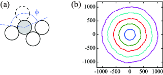
Figure 1: Off-lattice Eden model. (a) Sketch of the model. A new particle (dashed) is being added to its ancestor (shaded). In Alves et al.’s model [25, 27, 30], a random number for the angular position of the new particle is generated within $[\pi/6,\phi-\pi/6]$, where $\phi$ is defined in the sketch and $\pi/6$ is due to the finite radius of the new particle. In contrast, in our model, the random number is always drawn from $[0,2\pi)$ and then the attempt of generating the new particle is accepted with probability $(\phi-\pi/3)/2\pi$. (b) Typical cluster produced by our Eden model. The active particles, or the interface, at $t=405,803,1174,1592,1999$ are shown.

This model resembles the off-lattice Eden model studied by Alves et al. [25] (also described in [27, 30]) except for the criterion of the inner particles and for the way a new particle is added to the randomly chosen ancestor. On the former point, Alves et al. inactivated the particles inside a central core of radius $0.8\bar{r}$ [27, 30], where $\bar{r}$ is the mean distance of the particles on the interface from the origin, whereas in our model it is determined by the purely geometrical consideration, for which there is no risk of false inactivation. The latter point concerns the step (2) in the above procedure. When determining the direction to place a new particle, Alves et al. drew a random number from such angles that correspond to the empty neighborhood of the ancestor, while we always choose an angle within $[0,2\pi)$ and then judge whether the particle can be placed or not [figure 1(a)]. This guarantees local isotropy of the growth process. The author also considers that, in coarse-grained scales, it better corresponds to the growth of topological defects in the liquid-crystal turbulence [5, 6, 7].

The data presented below are obtained from 3000 independent simulations of the above-defined Eden model up to $t=1999$, which roughly corresponds to the final cluster size of $N=2\times 10^{6}$ if one does not discard the inner particles. Figure 1(b) shows a typical growing cluster; it displays the active particles at different times, labeled by $i$ below, which form the interface at each time by construction. The local interface height $h(x,t)$ is then determined from the distance $r_{i}$ between the origin and the active particle $i$ at a given angular position. More specifically, the full azimuthal range $[0,2\pi)$ is divided into $\lfloor 2\pi\langle r_{i}\rangle\rfloor$ bins, where $\langle r_{i}\rangle$ is the ensemble average of $r_{i}$, or the mean radius of the clusters at the given time, and $\lfloor\cdots\rfloor$ represents the integer part; then, for each bin and cluster, a single value of $h(x,t)$ is assigned as the mean of $r_{i}$ within the corresponding range of angular positions. Note that the width of the single bin is then roughly equal to the diameter of the particles. The lateral coordinate $x$ is defined along the mean shape of the clusters, i.e., the circle of circumference $2\pi\langle r_{i}\rangle$.

3 Results

We first check the scaling exponents $\alpha$ and $\beta$ by the usual method based on the Family-Vicsek scaling [31], which describes the spatial and temporal dependence of the roughness growth. To this end, we define the interface width $w(l,t)$ as the standard deviation of the height $h(x,t)$ measured over length $l$, or, more specifically, $w(l,t)\equiv\left\langle\sqrt{\langle\left[h(x,t)-\langle h(x,t)\rangle_{l}\right]^{2}\rangle_{l}}\right\rangle$ with the ensemble average $\langle\cdots\rangle$ and the average $\langle\cdots\rangle_{l}$ taken inside a segment of length $l$ around the position $x$. The Family-Vicsek scaling then reads

$$w(l,t)\sim t^{\beta}F_{w}(lt^{-1/z})\sim\cases{l^{\alpha}&for $l\ll l_{*}$,\\ t^{\beta}&for $l\gg l_{*}$,}$$ (2)

with $z\equiv\alpha/\beta$, a scaling function $F_{w}$ and a crossover length scale $l_{*}\sim t^{1/z}$. This relation is clearly confirmed in our numerical data, together with the KPZ-class exponent values $\alpha=1/2$, $\beta=1/3$ and $z=3/2$ (figure 2). The width $w(l,t)$ at fixed times grows as $w\sim l^{\alpha}$ with $\alpha=1/2$ for short length scales $l$, while it saturates at the value that increases with time [figure 2(a)]. This width at the largest length scale can be accurately measured by the overall width $W(t)\equiv\sqrt{\langle[h(x,t)-\langle h\rangle]^{2}\rangle}$, which indeed shows a clear power law $W\sim t^{\beta}$ with $\beta=1/3$ [figure 2(b)]. Note here that the overall width $W(t)$ should be measured with the ensemble average $\langle\cdots\rangle$ and not the spatial average taken for each interface, which turned out to bias the apparent value of $\beta$ as detailed in [7]. The agreement with the KPZ-class exponents is also checked by data collapse: the data for the width $w(l,t)$ at different times collapse reasonably well onto a single curve $F_{w}$ when $wt^{-\beta}$ is plotted against $lt^{-1/z}$ [insets of figure 2(a)].

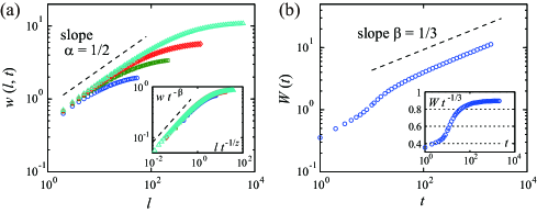
Figure 2: Family-Vicsek scaling. (a) Width $w(l,t)$ against length $l$ at different times $t=24,82,322,1999$ (from bottom to top). The inset shows the same data in the rescaled axes, $wt^{-\beta}$ vs $lt^{-1/z}$, with the KPZ-class exponents $\beta=1/3$ and $z=3/2$. (b) Overall width $W(t)$ against time $t$. The inset confirms the convergence to the asymptotic power law $W\sim t^{\beta}$ with $\beta=1/3$. The dashed lines are guides for the eyes indicating the slopes for the KPZ-class exponents.

The realization of the KPZ-class growth exponent $\beta=1/3$ implies that the local height $h$ of the interfaces can be described with a deterministic linear growth term and a stochastic $t^{1/3}$ term, as follows:

$$h\simeq v_{\infty}t+(\Gamma t)^{1/3}\chi,$$ (3)

where $v_{\infty}$ and $\Gamma$ denote two constant parameters and $\chi$ a random variable that captures the fluctuations of the growing interfaces. Note that we focus for the moment on asymptotic one-point statistics of the interface fluctuations and hence do not consider the dependence of $\chi$ on $x$ and $t$.

First we estimate the values of the two parameters $v_{\infty}$ and $\Gamma$, in the same manner as for the experiment on the liquid-crystal turbulence [5, 6, 7]. The linear growth rate $v_{\infty}$ is obtained as the asymptotic growth speed of the mean height. More specifically, since equation (3) indicates $\mathrm{d}\langle h\rangle/\mathrm{d}t\simeq v_{\infty}+c_{v}t^{-2/3}$ with a constant $c_{v}$, linear regression of the data for $\mathrm{d}\langle h\rangle/\mathrm{d}t$ against $t^{-2/3}$ in the asymptotic regime, here $t\geq 250$, provides a precise estimate of $v_{\infty}$ at $v_{\infty}=0.5139(2)$ [figure 3(a)]. Concerning the amplitude $\Gamma$ for the $t^{1/3}$-fluctuations, we use the relation to the second-order cumulant: ${\langle h^{2}\rangle}_{\rm c}\equiv W(t)^{2}\simeq(\Gamma t)^{2/3}{\langle\chi^{2}\rangle}_{\rm c}$. Setting the arbitrary variance of $\chi$ to that of the compared distribution function, namely the variance of the GUE Tracy-Widom distribution denoted by ${\langle\chi_{\rm GUE}^{2}\rangle}_{\rm c}$, we plot in figure 3(b) $({\langle h^{2}\rangle}_{\rm c}/{\langle\chi_{\rm GUE}^{2}\rangle}_{\rm c})^{3/2}/t$ and read its time asymptotic value. It shows a considerable finite-time effect, which is also visible in the overall width $W(t)$ [figure 2(b)]. Following the method used for the flat interfaces in the liquid-crystal experiment [7], we first fit a power law $a_{1}t^{-\delta}+a_{2}$ to the data for $t\geq 10$ in figure 3(b) and obtain $\delta=0.70(3)$. Since it is closest to $2/3$ among the multiples of $\beta=1/3$, we assume $\delta=2/3$ and fit again the data with a weight proportional to $(y-a_{2})^{-2}$, where $y$ is the ordinate of the data as shown in figure 3(b). This finally provides our estimate at $\Gamma=1.01(2)$. Note that the parameter values obtained here are connected to the three parameters in the KPZ equation (1) by $v_{\infty}=\lambda$ [29, 7] and $\Gamma=A^{2}|\lambda|/2$ with $A\equiv D/2\nu$ [10].

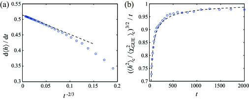
Figure 3: Parameter estimation. (a) Estimation of the linear growth rate $v_{\infty}$. The time derivative of the mean height, $\mathrm{d}\langle h\rangle/\mathrm{d}t$, is plotted against $t^{-2/3}$. The $y$-intercept of the linear regression (dashed line) provides the estimate of $v_{\infty}$. (b) Estimation of the amplitude $\Gamma$ for the $t^{1/3}$-fluctuations. The time-series of the second-order cumulant ${\langle h^{2}\rangle}_{\rm c}$ is displayed in such a way that the value of $\Gamma$ is found in the limit $t\to\infty$. It is obtained by fitting $at^{-2/3}+\Gamma$ (dashed line) to the data for $t\geq 10$ in order to take into account the finite-time effect (see text).

Using the measured parameter values, we rescale the height $h(x,t)$ in such a way to extract the random variable $\chi$:

$$q\equiv\frac{h-v_{\infty}t}{(\Gamma t)^{1/3}}\simeq\chi.$$ (4)

Figure 4(a) displays the histograms of the rescaled height $q$ at different times (symbols) and compare them with the GUE and GOE Tracy-Widom distributions (dashed and dotted lines, respectively). The data at the later time clearly indicate the GUE Tracy-Widom distribution, in agreement with the recent analytical results for the curved interfaces in the solvable models [10, 11, 12]. This is more quantitatively checked by plotting the difference in the $n$th-order cumulant, ${\langle q^{n}\rangle}_{\rm c}-{\langle\chi_{\rm GUE}^{n}\rangle}_{\rm c}$, in figure 4(b). We thereby confirm that the circular interfaces of our off-lattice Eden model indeed belong to the KPZ universality class at the level of the one-point distribution function. Moreover, the differences in the $n$th-order cumulants also measure the finite-time corrections toward this asymptotic distribution, which turn out to decay as $|{\langle q^{n}\rangle}_{\rm c}-{\langle\chi_{\rm GUE}^{n}\rangle}_{\rm c}|\sim t^{-2/3}$ for $n=1$ and $2$ [figure 4(c,d)]. The power-law decay $t^{-2/3}$ for the second-order cumulant has also been reported in all the previously studied systems [32, 33, 13, 14, 7]. In contrast, noteworthy is the decay $t^{-2/3}$ found for the first-order cumulant, or the mean, because the typical leading correction shown by the previous studies is $t^{-1/3}$, both for the solvable models [32, 33, 13, 14] and for the liquid-crystal experiment [5, 6, 7]. On the one hand, one cannot exclude the possibility that the correction in our case shows a crossover from $t^{-2/3}$ to $t^{-1/3}$ at larger times, as reported in simulations of flat interfaces in the discretized KPZ equation [34]. On the other hand, our result may indicate that our Eden model is endowed with some kind of symmetry, for which the leading correction term $t^{-1/3}$ for the mean vanishes. Note also that Alves et al. [25] numerically found the GUE Tracy-Widom distribution in their off-lattice Eden model, as well as in two on-lattice isotropic Eden models, and reported finite-time corrections for the mean proportional to $t^{-1/3}$. This difference should arise from the different definitions of the off-lattice Eden model as described in the previous section.

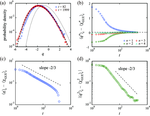
Figure 4: One-point distribution and finite-time corrections. (a) Histogram of the rescaled local height $q\equiv(h-v_{\infty}t)/(\Gamma t)^{1/3}$ for $t=82$ (blue circles) and $t=1999$ (red diamonds). The dashed line indicates the GUE Tracy-Widom distribution expected for the curved interfaces, whereas the dotted line shows the appropriately rescaled GOE Tracy-Widom distribution for the flat interfaces. (b) Finite-time corrections in the $n$th-order cumulants. Shown are the differences between the cumulants of the measured rescaled height $q$ and the theoretical values for the GUE Tracy-Widom distribution. (c,d) Corrections in the first- and second-order cumulants [same data as (b)] shown in the double logarithmic scales. The dashed lines are guides for the eyes, both indicating the slope $-2/3$.

The spatial correlation function

$$C_{\rm s}(l;t)\equiv\langle h(x+l,t)h(x,t)\rangle-\langle h(x+l,t)\rangle\langle h(x,t)\rangle.$$ (5)

is also a quantity of central interest in the recent analytical studies [10, 11, 12]. For the solved cases of the curved interfaces, it has been shown to coincide with the covariance of the stochastic process called the Airy₂ process $\mathcal{A}_{2}(t^{\prime})$ [35], which was noticed to be equivalent to the dynamics of the largest eigenvalue in Dyson’s Brownian motion for GUE random matrices [36]. The prediction reads

$$C_{\rm s}(l;t)\simeq(\Gamma t)^{2/3}g_{2}\left(\frac{Al}{2}(\Gamma t)^{-2/3}\right)$$ (6)

with $g_{2}(\zeta)\equiv\langle\mathcal{A}_{2}(t^{\prime}+\zeta)\mathcal{A}_{2}(t^{\prime})\rangle$, which was indeed substantiated in the liquid-crystal experiment [5, 7]. Our numerical data also confirm this in the time asymptotic limit, as shown in figure 5(a) which displays the rescaled correlation function $C^{\prime}_{\rm s}(\zeta;t)\equiv C_{\rm s}(l;t)/(\Gamma t)^{2/3}$ against $\zeta\equiv(Al/2)(\Gamma t)^{-2/3}$. The finite-time correction is also quantified by measuring the integral $C_{\rm s}^{\rm int}(t)\equiv\int_{0}^{\infty}C^{\prime}_{\rm s}(\zeta;t)\mathrm{d}\zeta$ as a function of time. This indeed approaches the value for the Airy₂ covariance $g_{2}^{\rm int}\equiv\int_{0}^{\infty}g_{2}(\zeta)\mathrm{d}\zeta$ by a power law $g_{2}-C_{\rm s}^{\rm int}(t)\sim t^{-1/3}$ [figure 5(b)], which was also identified in the liquid-crystal experiment [5, 7].

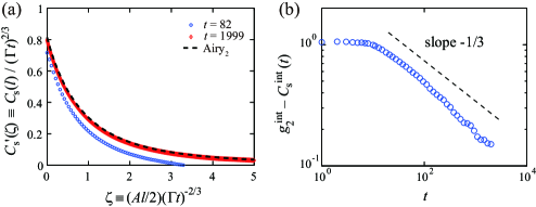
Figure 5: Spatial correlation function $C_{\rm s}(l;t)$. (a) Rescaled correlation function $C^{\prime}_{\rm s}(\zeta;t)\equiv C_{\rm s}(l;t)/(\Gamma t)^{2/3}$ against rescaled length $\zeta\equiv(Al/2)(\Gamma t)^{-2/3}$. The symbols show the results for the Eden model at $t=82$ (blue circles) and $t=1999$ (red diamonds), while the dashed line indicates the Airy₂ covariance $g_{2}(\zeta)$. (b) Finite-time correction in the integral of the rescaled correlation function $C_{\rm s}^{\rm int}(t)\equiv\int_{0}^{\infty}C^{\prime}_{\rm s}(\zeta;t)\mathrm{d}\zeta$. Displayed is the difference from the value for the Airy₂ covariance $g_{2}^{\rm int}\equiv\int_{0}^{\infty}g_{2}(\zeta)\mathrm{d}\zeta$ as a function of time. The dashed line is a guide for the eyes showing the slope $-1/3$.

From now on we study statistical quantities that remain out of reach of rigorous theoretical treatment so far. Among them particularly important are those characterizing the correlation in time, especially the temporal correlation function

$$C_{\rm t}(t,t_{0})\equiv\langle h(x,t)h(x,t_{0})\rangle-\langle h(x,t)\rangle\langle h(x,t_{0})\rangle.$$ (7)

The temporal correlation should be measured along the directions in which fluctuations propagate in space-time, called the characteristic lines [37, 38]. In our case these are simply the radial directions of the circular growth and represented by the fixed $x$ in equation (7).

For the circular case, Singha [39] performed an approximative theoretical calculation based on the assumption of effectively linear evolution of the height fluctuations, and derived

$$\frac{C_{\rm t}(t,t_{0})}{C_{\rm t}(t_{0},t_{0})}\approx F_{\rm Singha}(t/t_{0};b),$$ (8)

$$F_{\rm Singha}(x;b)\equiv\frac{\rme^{b(1-1/\sqrt{x})}\Gamma(2/3,b(1-1/\sqrt{x}))}{\Gamma(2/3)},$$ (9)

with a single unknown parameter $b$, the upper incomplete Gamma function $\Gamma(s,x)\equiv\int_{x}^{\infty}y^{s-1}\rme^{-y}\mathrm{d}y$ and the Gamma function $\Gamma(s)=\Gamma(s,0)$. For the liquid-crystal experiment [7], this functional form works only asymptotically. More specifically, it fits the experimental data for $t>t_{0}$ on condition that the right hand side of equation (8) is multiplied by a time-dependent coefficient $c(t_{0})$, which turned out to satisfy $c(t_{0})\to 1$ with $t_{0}\to\infty$ and is attributed, somewhat speculatively, to microscopic dynamics of the liquid-crystal convection. On the other hand, Singha himself checked his prediction by simulations of the conventional on-lattice Eden model [39]. He then found good agreement if an independent value of $b$ is chosen for each growth direction, without however studying the dependence on $t_{0}$.

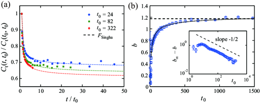
Figure 6: Temporal correlation function $C_{\rm t}(t,t_{0})$. (a) $C_{\rm t}(t,t_{0})/C_{\rm t}(t_{0},t_{0})$ against $t/t_{0}$ with different $t_{0}$ (as shown in the legend). The dashed lines show the results of fitting by Singha’s function (9). Notice that the correlation function remains far above zero. (b) The values of the fitting parameter $b$ in equation (8) as a function of $t_{0}$. The dashed line indicates the mean value of $b$ estimated for $t\geq 500$, while the dotted curve shows the result of a power-law fit $b(t_{0})=at_{0}^{-\delta}+b_{\infty}$. The inset displays the quality of this power-law fit in the axes $b_{\infty}-b$ vs $t_{0}$, with a guide for the eyes indicating the slope for $\delta=1/2$.

The temporal correlation function is measured in our off-lattice Eden model and shown in figure 6(a), together with the results of fitting by Singha’s function (9). As shown in the figure, Singha’s function fits our data reasonably well within the whole time window, or $c(t_{0})=1$ for all $t_{0}$, in agreement with his simulations for the on-lattice Eden model. We however find that the value of the parameter $b$ obtained by the best fitting of the data increases with $t_{0}$ [figure 6(b)]. Assuming the convergence of $b$ at later times such as $t\geq 500$, we estimate the asymptotic value of $b$ at $b=1.18(3)$. On the other hand, attempt of a power-law fit in the form $b(t_{0})=at_{0}^{-\delta}+b_{\infty}$ yields a reasonable result with $b_{\infty}=1.27(3)$ [dotted curve and inset of figure 6(b)]. Given large uncertainties expected in the nonlinear fit of $F_{\rm Singha}$, especially for later times $t_{0}$, here we do not single out either possibility but instead provide a single final estimate $b=1.22(8)$ that covers both confidence intervals. In any case, our results indicate that Singha’s function (9) indeed explains the global form of the temporal correlation function in our Eden model. This implies in particular that positive correlation would remain forever, i.e., $\displaystyle{\lim_{t\to\infty}C_{\rm t}(t,t_{0})\sim t_{0}^{2/3}>0}$, which was also inferred for the circular interfaces in the liquid-crystal experiment [7]. Note that, for the flat interfaces, the temporal correlation was shown to decay to zero as $C_{\rm t}(t,t_{0})\sim t^{-2/3}$ for fixed $t_{0}$, both numerically [40] and experimentally [7]. Concerning the other limit $t\to t_{0}$, equations (8) and (9) with $C_{\rm t}(t_{0},t_{0})=W(t_{0})^{2}\simeq(\Gamma t_{0})^{2/3}{\langle\chi_{\rm GUE}^{2}\rangle}_{\rm c}$ yield

$$C_{\rm t}(t,t_{0})\simeq(\Gamma^{2}t_{0}t)^{1/3}{\langle\chi^{2}\rangle}_{\rm c}\left[1-\frac{R}{2}\left(1-\frac{t_{0}}{t}\right)^{2/3}\right]\quad(t-t_{0}\ll t_{0})$$ (10)

with $R/2\approx 3b^{2/3}/2^{5/3}\Gamma(2/3)$ [39]. Our data indeed confirm this functional form (figure 7), except that they indicate $R/2\approx 0.68$ rather than $R/2\approx 3b^{2/3}/2^{5/3}\Gamma(2/3)=0.80(3)$. This implies that Singha’s function (9) is not quantitatively precise in the short-time regime $t-t_{0}\ll t_{0}$ of the temporal correlation function.

In relation to the liquid-crystal experiment, our data for the Eden model do not require the extra multiplier $c(t_{0})$ in equation (8), which was necessary for the experimental data [7]. This supports the author’s speculation [7] that the need for the coefficient $c(t_{0})$ for the experiment results from microscopic dynamics of the liquid-crystal convection decoupled from the interface growth, which is obviously missing in the Eden model. With this difference in mind, the liquid-crystal experiment gave $b\approx 0.8(1)$ and $R/2\approx 0.6$, to be compared with $b=1.22(8)$ and $R/2\approx 0.68$ in our Eden model. This suggests that the parameter $b$ is not a universal quantity of the KPZ class.

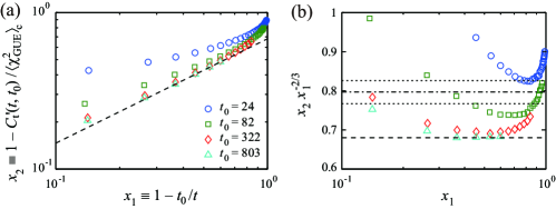
Figure 7: Short-time behavior of the temporal correlation function $C_{\rm t}(t,t_{0})$. (a) $x_{2}\equiv 1-C^{\prime}_{\rm t}(t,t_{0})/{\langle\chi_{\rm GUE}^{2}\rangle}_{\rm c}$ against $x_{1}\equiv 1-t_{0}/t$ with $C^{\prime}_{\rm t}(t,t_{0})\equiv C_{\rm t}(t,t_{0})/(\Gamma^{2}t_{0}t)^{1/3}$ for different reference times $t_{0}$. (b) Same data in the different axes $x_{2}x_{1}^{-2/3}$ vs $x_{1}$. The dashed lines in both panels show the right hand side of equation (10) with $R/2=0.68$. The dashed-dotted and dotted lines in the panel (b) indicate the value and the confidence interval, respectively, of $3b^{2/3}/2^{5/3}\Gamma(2/3)=0.80(3)$.

Next we turn our attention to another aspect of the temporal correlation, namely the first-passage property characterized by the temporal persistence probability $P_{\pm}(t,t_{0})$. For the fluctuating interfaces, $P_{\pm}(t,t_{0})$ is defined as the joint probability that the interface fluctuation $\delta h(x,t)\equiv h(x,t)-\langle h\rangle$ at a fixed location is positive (negative) at time $t_{0}$ and maintains the same sign until time $t$ [40, 39]. Here we distinguish the positive and negative fluctuations denoted by $+$ and $-$, respectively, because Kallabis and Krug numerically found power-law decay $P_{\pm}(t,t_{0})\sim t^{-\theta_{\pm}}$ with different exponent values, $\theta_{+}<\theta_{-}$ if $\lambda>0$ and opposite in the other case, in the case of flat interfaces [40]. This asymmetry was also confirmed in the liquid-crystal experiment for the flat interfaces, while no asymmetry was identified for the circular case [7]. Our numerically produced circular interfaces also support this claim, as summarized in figure 8. In the main panels, we find power-law decay

$$P_{\pm}(t,t_{0})\sim(t/t_{0})^{-\theta_{\pm}}$$ (11)

for sufficiently large $t/t_{0}$. This is further confirmed in the insets, where the running exponents $-\theta_{\pm}(t,t_{0})\equiv\mathrm{d}[\log P_{\pm}(t,t_{0})]/\mathrm{d}[\log(t/t_{0})]$ with different $t_{0}$ overlap reasonably well when plotted against $t/t_{0}$ and converge to constants for large abscissae. Fitting the data within this plateau regime (not only for the three $t_{0}$ in figure 8), we obtain $\theta_{+}=0.81(3)$ and $\theta_{-}=0.77(4)$. This is in good agreement with the experimentally found values of $\theta_{+}=0.81(2)$ and $\theta_{-}=0.80(2)$ for the circular interfaces and significantly different from those for the flat interfaces, $\theta_{+}=1.35(5)$ and $\theta_{-}=1.85(10)$ [7]. Our result confirms in particular the absence of the asymmetry between the positive and negative fluctuations for the circular interfaces, i.e., $\theta_{+}=\theta_{-}$ in our precision. The asymmetry $\theta_{+}\neq\theta_{-}$ present for the flat interfaces has been attributed to the nonlinear term of the KPZ equation (1) [40]; understanding how this effect is cancelled for the circular interfaces is an interesting problem left for future studies.

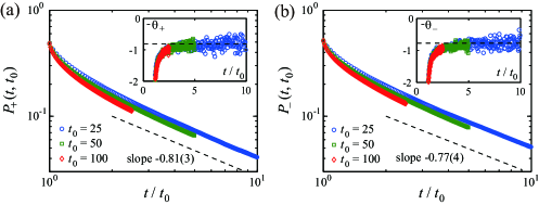
Figure 8: Temporal persistence probability $P_{\pm}(t,t_{0})$ for the positive (a) and negative (b) fluctuations, with different $t_{0}$ as shown in the legends. The insets show the running exponents $-\theta_{\pm}(t,t_{0})\equiv\mathrm{d}[\log P_{\pm}(t,t_{0})]/\mathrm{d}[\log(t/t_{0})]$. The dashed lines show the estimated values of the persistence exponents, $\theta_{+}=0.81(3)$ and $\theta_{-}=0.77(4)$.

The notion of the persistence can also be considered in space [41, 42]. It is then characterized by the spatial persistence probability $P_{\pm}^{\rm(s)}(l;t)$, which is the probability that a fluctuation remains positive or negative over length $l$ in a spatial profile of the interfaces at time $t$. Although a few analytical and numerical studies have shown nontrivial character of the spatial persistence for the stationary interfaces [41, 42], for the growing interfaces it has been studied only experimentally so far, in the liquid-crystal experiment [7] and in an earlier experiment on paper smoldering [43] which also exhibited the KPZ scaling exponents [44]. Interestingly, the two experiments showed different results: exponential decay for the liquid-crystal turbulence and power-law decay $P_{\pm}^{\rm(s)}(l;t)\sim l^{-1/2}$ for the paper smoldering. The spatial persistence is therefore measured in our Eden model and yields the results shown in figure 9. We then find clear exponential decay for both positive and negative fluctuations,

$$P_{\pm}^{\rm(s)}(l;t)\sim\rme^{-\kappa^{\rm(s)}_{\pm}\zeta},$$ (12)

with values of $\kappa^{\rm(s)}_{\pm}$ independent of $t$ when plotted against the dimensionless length scale $\zeta\equiv(Al/2)(\Gamma t)^{-2/3}$. Measuring them at the latest two times at which the interface profiles were recorded, namely $t=1717$ and $1999$, we obtain estimates of $\kappa^{\rm(s)}_{+}=0.90(2)$ and $\kappa^{\rm(s)}_{-}=0.89(4)$ for our Eden model. They are in excellent agreement with the values numerically obtained for the temporal persistence of GUE Dyson’s Brownian motion, $\kappa^{\rm(s)}_{+}=0.90(8)$ and $\kappa^{\rm(s)}_{-}=0.90(6)$ [7], which is expected to be equivalent to the spatial profile of the curved KPZ-class interfaces. This is therefore evidence for universal spatial persistence in the growth regime of the KPZ class, which in fact concerns infinite-point correlation in the spatial profile. It is also noteworthy that the positive and negative fluctuations show no asymmetry in this spatial persistence either. Similar values were also reported in the liquid-crystal experiment, $\kappa^{\rm(s)}_{+}=1.07(8)$ and $\kappa^{\rm(s)}_{-}=0.87(6)$ [7], albeit with a small difference in the former which is probably due to finite-time effect but should be clarified by further study. In passing, for the flat interfaces, the liquid-crystal experiment showed $\kappa^{\rm(s)}_{+}=1.9(3)$ and $\kappa^{\rm(s)}_{-}=2.0(3)$ [7], which are significantly different from the values of the circular case.

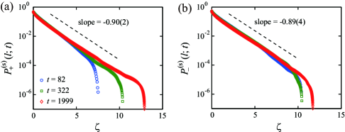
Figure 9: Spatial persistence probability $P_{\pm}^{\rm(s)}(l;t)$ for the positive (a) and negative (b) fluctuations, with different $t$ as shown in the legends. The length $l$ is shown in the rescaled unit $\zeta\equiv(Al/2)(\Gamma t)^{-2/3}$. The dashed lines are guides for the eyes showing the estimated values of $\kappa^{\rm(s)}_{+}$ and $\kappa^{\rm(s)}_{-}$.

We finally study extreme-value statistics for the interface fluctuations with our numerical data. Specifically, we focus on the maximal height $H_{\rm max}$ measured with respect to a fictitious substrate that extends from the origin [figure 10(a)], which is known to obey, asymptotically, the GOE Tracy-Widom distribution by studies of solvable models [36, 45, 46, 47, 48]. This is the same distribution as for the one-point distribution of the flat interfaces and differs from the GUE Tracy-Widom distribution for that of the circular interfaces. For our Eden model, we measure this maximal height directly by $H_{\rm max}=\max y^{\prime}_{i}$, where $i$ denotes the index of the active particles and $(x^{\prime},y^{\prime})$ the coordinates defined with respect to the substrate [figure 10(a)]. Statistics of $H_{\rm max}$ is improved by rotating the substrate, or the frame $(x^{\prime},y^{\prime})$, arbitrarily around the origin. The obtained histograms are shown in figure 10(b) for the rescaled maximal height $q_{\rm max}^{\rm(h)}\equiv(H_{\rm max}-v_{\infty}t)/(\Gamma t)^{1/3}$, which clearly confirm the asymptotic GOE Tracy-Widom distribution for this quantity. Moreover, in figure 10(c,d), we measure the finite-time corrections in the $n$th-order cumulants ${\langle(q_{\rm max}^{\rm(h)})^{n}\rangle}_{\rm c}$ and find ${\langle q_{\rm max}^{\rm(h)}\rangle}_{\rm c}-{\langle\chi_{\rm GOE}\rangle}_{\rm c}\sim t^{-2/3}$ for the mean, in contrast with $t^{-1/3}$ found for the liquid-crystal experiment [7]. Since the same set of the different exponents has been found for the finite-time correction in the one-point distribution, the author believes that the leading correction terms $t^{-1/3}$ for the mean of both distributions vanish for the same reason in our Eden model.

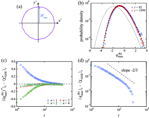
Figure 10: Maximal height distribution. (a) Definition of the maximal height $H_{\rm max}$. The origin of the frame $(x^{\prime},y^{\prime})$ is fixed at the position of the initial seed of the cluster. Shown in purple are the active particles of a cluster at $t=1999$, which is also displayed in figure 1(b). (b) Histogram of the rescaled maximal height $q^{\rm(h)}_{\rm max}\equiv(H_{\rm max}-v_{\infty}t)/(\Gamma t)^{1/3}$ for $t=82$ (blue circles) and $t=1999$ (red diamonds). The dashed and dotted lines indicate the GOE and GUE Tracy-Widom distributions, respectively. Note that the conventional definition of the GOE TW random variable is multiplied by $2^{-2/3}$, in view of the theoretical results for the solvable models [36, 45, 46, 47, 48]. (c) Finite-time corrections in the $n$th-order cumulants. Shown are the differences between the cumulants of the measured $q^{\rm(h)}_{\rm max}$ and the theoretical values for the GOE Tracy-Widom distribution. (d) Correction in the first-order cumulant [same data as (c)] shown in the double logarithmic scales. The dashed line is a guide for the eyes indicating the slope $-2/3$.

4 Summary

In the present paper, we have introduced an off-lattice variant of the Eden model and determined the statistical properties of its circular interfaces, as a numerical case study for the $(1+1)$-dimensional KPZ universality class. Besides confirming the universal distribution function and the spatial correlation function in agreement with the analytical results on the solvable models, namely the GUE Tracy-Widom distribution and the Airy₂ covariance, our particular focus has been put on the unsolved statistical properties such as the temporal correlation function and the persistence probability in space and time. Good agreement is then found with the recent experiment on the growing interfaces in the liquid-crystal turbulence, as far as characteristic quantities are compared such as the temporal persistence exponent $\theta_{\pm}$ and the exponential decay rate $\kappa_{\pm}^{\rm(s)}$ for the spatial persistence. In particular, unlike the flat interfaces, we have demonstrated that $\theta_{+}=\theta_{-}$ holds for the circular case, supporting one of the conclusions reached in the liquid-crystal experiment. The temporal correlation function has also been shown to fit Singha’s approximative functional form (8) and (9) without the small modification required for the liquid-crystal experiment. This indicates that the circular interfaces have long-lasting temporal correlation, i.e., $C_{\rm t}(t,t_{0})>0$ for large $t$, presumably even in the limit $t\to\infty$ unlike the flat interfaces. These agreements with the experimental results for the circular case and the sharp contrast to the flat interfaces (see table 1 of [7] for a summary) further emphasize the geometry-dependent universality of the $(1+1)$-dimensional KPZ class.

In view of these experimental and numerical results for the universality beyond the analytically solved quantities, it would be important to provide firmer theoretical grounds for such unsolved universal statistical properties, especially those related to the temporal correlation. This would call for several complementary approaches: attempts to provide analytical solutions for those quantities in solvable models, refinement of approximative theoretical evaluation performed by Singha [39], and recent developments in the application of renormalization group techniques [49, 50, 51] are also intriguing. Combination of such theoretical approaches as well as further experimental and numerical case studies would surely help understand this prominent out-of-equilibrium universality of the KPZ class, which governs the general phenomenon of the growing interfaces.

References

References

- [1] Barabasi A L and Stanley H E 1995 Fractal Concepts in Surface Growth (Cambridge: Cambridge Univ. Press)
- [2] Kardar M, Parisi G and Zhang Y C 1986 Phys. Rev. Lett. 56 889–892
- [3] Forster D, Nelson D R and Stephen M J 1977 Phys. Rev. A 16 732–749
- [4] van Beijeren H, Kutner R and Spohn H 1985 Phys. Rev. Lett. 54 2026–2029
- [5] Takeuchi K A and Sano M 2010 Phys. Rev. Lett. 104 230601
- [6] Takeuchi K A, Sano M, Sasamoto T and Spohn H 2011 Sci. Rep. 1 34
- [7] Takeuchi K A and Sano M 2012 arXiv 1203.2530
- [8] Johansson K 2000 Commun. Math. Phys. 209 437–476
- [9] Baik J, Deift P and Johansson K 1999 J. Am. Math. Soc. 12 1119–1178
- [10] Kriecherbauer T and Krug J 2010 J. Phys. A 43 403001
- [11] Sasamoto T and Spohn H 2010 J. Stat. Mech. 2010 P11013
- [12] Corwin I 2012 Random Matrices: Theory and Applications 1 1130001
- [13] Sasamoto T and Spohn H 2010 Phys. Rev. Lett. 104 230602
- [14] Sasamoto T and Spohn H 2010 Nucl. Phys. B 834 523–542
- [15] Amir G, Corwin I and Quastel J 2011 Commun. Pure Appl. Math. 64 466–537
- [16] Calabrese P, Le Doussal P and Rosso A 2010 Europhys. Lett. 90 20002
- [17] Dotsenko V 2010 Europhys. Lett. 90 20003
- [18] Calabrese P and Le Doussal P 2011 Phys. Rev. Lett. 106 250603
- [19] Imamura T and Sasamoto T 2011 arXiv 1111.4634
- [20] Prähofer M and Spohn H 2000 Phys. Rev. Lett. 84 4882–4885
- [21] Tracy C A and Widom H 1994 Commun. Math. Phys. 159 151–174
- [22] Eden M 1961 A two-dimensional growth process Proceedings of the Fourth Berkeley Symposium on Mathematical Statistics and Probability, Volume 4: Contributions to Biology and Problems of Medicine (Berkeley: Univ. of California Press) pp 223–239
- [23] Freche P, Stauffer D and Stanley H E 1985 J. Phys. A 18 L1163–L1168
- [24] Paiva L R and Ferreira Jr S C 2007 J. Phys. A 40 F43–F49
- [25] Alves S G, Oliveira T J and Ferreira S C 2011 Europhys. Lett. 96 48003
- [26] Wang C Y, Liu P L and Bassingthwaighte J B 1995 J. Phys. A 28 2141
- [27] Ferreira Jr S C and Alves S G 2006 J. Stat. Mech. 2006 P11007
- [28] Kuennen E W and Wang C Y 2008 J. Stat. Mech. 2008 P05014
- [29] Krug J, Meakin P and Halpin-Healy T 1992 Phys. Rev. A 45 638–653
- [30] Alves S G, Ferreira Jr S C and Martins M L 2008 Braz. J. Phys. 38 81–86
- [31] Family F and Vicsek T 1985 J. Phys. A 18 L75–L81
- [32] Ferrari P L and Frings R 2011 J. Stat. Phys. 144 1123–1150
- [33] Baik J and Jenkins R 2011 arXiv 1111.0269
- [34] Oliveira T J, Ferreira S C and Alves S G 2012 Phys. Rev. E 85 010601
- [35] Prähofer M and Spohn H 2002 J. Stat. Phys. 108 1071–1106
- [36] Johansson K 2003 Commun. Math. Phys. 242 277–329
- [37] Ferrari P L 2008 J. Stat. Mech. 2008 P07022
- [38] Corwin I, Ferrari P L and Péché S 2012 Ann. Inst. H. Poincaré B Probab. Statist. 48 134–150
- [39] Singha S B 2005 J. Stat. Mech. 2005 P08006
- [40] Kallabis H and Krug J 1999 Europhys. Lett. 45 20
- [41] Majumdar S N and Bray A J 2001 Phys. Rev. Lett. 86 3700–3703
- [42] Constantin M, Das Sarma S and Dasgupta C 2004 Phys. Rev. E 69 051603
- [43] Merikoski J, Maunuksela J, Myllys M, Timonen J and Alava M J 2003 Phys. Rev. Lett. 90 024501
- [44] Maunuksela J, Myllys M, Kähkönen O P, Timonen J, Provatas N, Alava M J and Ala-Nissila T 1997 Phys. Rev. Lett. 79 1515–1518
- [45] Forrester P J, Majumdar S N and Schehr G 2011 Nucl. Phys. B 844 500–526
- [46] Corwin I, Quastel J and Remenik D 2011 arXiv 1106.2717
- [47] Liechty K 2011 arXiv 1111.4239
- [48] Schehr G 2012 arXiv 1203.1658
- [49] Canet L, Chaté H, Delamotte B and Wschebor N 2010 Phys. Rev. Lett. 104 150601
- [50] Canet L, Chaté H, Delamotte B and Wschebor N 2011 Phys. Rev. E 84 061128
- [51] Corwin I and Quastel J 2011 arXiv 1103.3422
- [52] Bornemann F 2010 Math. Comput. 79 871–915