Random walks on temporal networks
Abstract
Many natural and artificial networks evolve in time. Nodes and connections appear and disappear at various timescales, and their dynamics has profound consequences for any processes in which they are involved. The first empirical analysis of the temporal patterns characterizing dynamic networks are still recent, so that many questions remain open. Here, we study how random walks, as paradigm of dynamical processes, unfold on temporally evolving networks. To this aim, we use empirical dynamical networks of contacts between individuals, and characterize the fundamental quantities that impact any general process taking place upon them. Furthermore, we introduce different randomizing strategies that allow us to single out the role of the different properties of the empirical networks. We show that the random walk exploration is slower on temporal networks than it is on the aggregate projected network, even when the time is properly rescaled. In particular, we point out that a fundamental role is played by the temporal correlations between consecutive contacts present in the data. Finally, we address the consequences of the intrinsically limited duration of many real world dynamical networks. Considering the fundamental prototypical role of the random walk process, we believe that these results could help to shed light on the behavior of more complex dynamics on temporally evolving networks.
pacs:
05.40.Fb, 89.75.Hc, 89.75.-kI Introduction
Many real networks are dynamic structures in which connections appear, disappear, or are rewired on various timescales Holme and Saramäki (2011). For example, the links representing social relationships in social networks Wasserman and Faust (1994) are a static representation of a succession of contact or communication events, which are constantly created or terminated between pairs of individuals (actors). Such temporal evolution is an intrinsic feature of many natural and artificial networks, and can have profound consequences for the dynamical processes taking place upon them. Until recently however, a large majority of studies about complex networks have focused on a static or aggregated representation, in which all the links that appeared at least once coexist. This is the case, for example, in the seminal works on scientific collaboration networks Newman (2001), or on movie costarring networks Barabási and Albert (1999). In particular, dynamical processes have mainly been studied on static complex networks Barrat et al. (2008).
In recent years, the interest towards the temporal dimension of the network description has blossomed. Empirical analyses have revealed rich and complex patterns of dynamic evolution Hui et al. (2005); Holme (2005); Onnela et al. (2007); Gautreau et al. (2009); Cattuto et al. (2010); Tang et al. (2010a); Bajardi et al. (2011); Stehlé et al. (2011a); Miritello et al. (2011); Karsai et al. (2011); Holme and Saramäki (2011), pointing out the need to characterize and model them Scherrer et al. (2008); Hill and Braha (2010); Gautreau et al. (2009); Stehlé et al. (2010); Zhao et al. (2011). At the same time, researchers have started to study how the temporal evolution of the network substrate impacts the behavior of dynamical processes such as epidemic spreading Rocha et al. (2011); Isella et al. (2011); Stehlé et al. (2011a); Karsai et al. (2011); Miritello et al. (2011); Kivela et al. (2011), synchronization Fujiwara et al. (2011), percolation Parshani et al. (2010); Bajardi et al. (2011) and social consensus Baronchelli and Díaz-Guilera (2012).
Here, we focus on the dynamics of a random walker exploring a temporal network Weiss (1994); Hughes (1995); Lovász (1996). The random walk is indeed the simplest diffusion model, and its dynamics provides fundamental hints to understand the whole class of diffusive processes on networks. Moreover, it has relevant applications in such contexts as spreading dynamics (i.e. virus or opinion spreading) and searching. For instance, assuming that each vertex knows only about the information stored in each of its nearest neighbors, the most naive economical strategy is the random walk search, in which the source vertex sends one message to a randomly selected nearest neighbor Adamic et al. (2001); Lv et al. (2002); Barrat et al. (2008). If that vertex has the information requested, it retrieves it; otherwise, it sends a message to one of its nearest neighbors, until the message arrives to its finally target destination. Thus, the random walk represents a lower bound on the effects of searching in the absence of any information in the network, apart form the purely local information about the contacts at a given instant of time.
In our study, we consider as typical examples of temporal networks the dynamical sequences of contact between individuals in various social contexts, as recorded by the SocioPatterns project Soc ; Cattuto et al. (2010). These datasets contain indeed the time-resolved patterns of face-to-face co-presence of individuals in settings such as conferences, with high temporal resolution: for each contact between individuals, the starting and ending times are registered by the measuring infrastructure, giving access to the timing and duration of contacts.
The paper is structured as follows. In Sec II we review some of the fundamental results for random walks on static networks. In Sec. III we describe the empirical dynamical networks considered: we recall some basic definitions, present an analysis of the datasets, and introduce suitable randomization procedures, which will help later on to pinpoint the role of the correlations in the real data. In Sec. IV we write down mean-field equations for the case of maximally randomized dynamical contact networks, and in Sec. V we investigate the random walk dynamics numerically, focusing on the exploration properties and on the mean first passage times. Sec. VI is devoted to the analysis of the impact of the finite temporal duration of real time series. Finally, we summarize our results and comment on some perspectives in Sec VII.
II A short overview of random walks on static networks
The random walk (RW) process is defined by a walker that, located on a given vertex at time , hops to a nearest neighbor vertex at time .
In binary networks, defined by the adjacency matrix such that is is a neighbor of , and else, the transition probability at each time step from to is
| (1) |
where is the degree of vertex : the walker hops to a nearest neighbor of , chosen uniformly at random among the neighbors, hence with probability (note that we consider here undirected networks with , but the process can be considered as well on directed networks). In weighted networks with a weight matrix , the transition probability takes instead the form
| (2) |
where is the strength of vertex Barrat et al. (2004). Here the walker chooses a nearest neighbor with probability proportional to the weight of the corresponding connecting edge.
The basic quantity characterizing random walks in networks is the occupation probability , defined as the steady state probability (i.e., measured in the infinite time limit) that the walker occupies the vertex , or in other words, the steady state probability that the walker will land on vertex after a jump from any other vertex. Following rigorous master equation arguments, it is possible to show that the occupation probability takes the form Noh and Rieger (2004); Wu et al. (2007)
| (3) |
respectively in binary and weighted networks.
Other characteristic properties of the random walk, relevant to the properties of searching in networks, are the mean first-passage time (MFPT) and the coverage Weiss (1994); Hughes (1995); Lovász (1996). The MFPT of a node is defined as the average time taken by the random walker to arrive for the first time at , starting from a random initial position in the network. This definition gives the number of messages that have to be exchanged, on average, in order to find vertex . The coverage , on the other hand, is defined as the number of different vertices that have been visited by the walker at time , averaged for different random walks starting from different sources. The coverage can thus be interpreted as the searching efficiency of the network, measuring the number of different individuals that can be reached from an arbitrary origin in a given number of time steps.
At a mean-field level, these quantities are computed as follows: let us define as the probability for the walker to arrive for the first time at vertex in time steps. Since in the steady state is reached in a jump with probability , we have . The MFPT to vertex can thus be estimated as the average , leading to
| (4) |
On the other hand, we can define the random walk reachability of vertex , , as the probability that vertex is visited by a random walk starting at an arbitrary origin, at any time less than or equal to . The reachability takes the form
| (5) |
where the last expression is valid in the limit of sufficiently small . The coverage of a random walk at time will thus be given by the sum of these probabilities, i.e.
| (6) |
For sufficiently small , the exponential in Eq. (6) can be expanded to yield , a linear coverage implying that at the initial stages of the walk, a different vertex is visited at each time step, independently of the network properties Stauffer and Sahimi (2005); Almaas et al. (2003).
It is now important to note that the random walk process has been defined here in a way such that the walker performs a move and changes node at each time step, potentially exploring a new node: except in the pathological case of a random walk starting on an isolated node, the walker has always a way to move out of the node it occupies. In the context of temporal networks, on the other hand, the walker might arrive at a node that at the successive time step becomes isolated, and therefore has to remain trapped on that node until a new link involving occurs. In order to compare in a meaningful way random walk processes on static and dynamical networks, and on different dynamical networks, we consider in each dynamical network the average probability that a node has at least one link. The walker is then expected to move on average once every time steps, so that we will consider the properties of the random walk process on dynamical networks as a function of the rescaled time .
III Empirical dynamical networks
III.1 Basics on temporal networks
Dynamical or temporal networks Holme and Saramäki (2011) are properly represented in terms of a contact sequence, representing the contacts (edges) as a function of time: a set of triplets where and are interacting at time , with , where is the total duration of the contact sequence. The contact sequence can thus be expressed in terms of a characteristic function (or temporal adjacency matrix Newman (2010)) , taking the value when actors and are connected at time , and zero otherwise.
Coarse-grained information about the structure of dynamical networks can be obtained by projecting them onto aggregated static networks, either binary or weighted. The binary projected network informs of the total number of contacts of any given actor, while its weighted version carries additional information on the total time spent in interactions by each actor Onnela et al. (2007); Holme and Saramäki (2011); Isella et al. (2011); Stehlé et al. (2011b). The aggregated binary network is defined by an adjacency matrix of the form
| (7) |
where is the Heaviside theta function defined by if and if . In this representation, the degree of vertex , , represents the number of different agents with whom agent has interacted. The associated weighted network, on the other hand, has weights of the form
| (8) |
Here, represents the number of interactions between agents and , normalized by its maximum possible value, i. e. the total duration of the contact sequence . The strength of vertex , , represents the average number of interactions of agent at each time step.
While static projections represent a first step in the understanding of the properties of dynamical networks, they coarse-grain a great deal of information from the empirical time series, a fact that can be particularly relevant when considering dynamical processes running on top of dynamical networks Isella et al. (2011). At a basic topological level, projected networks disregard the fact that dynamics on temporal networks are in general restricted to follow time respecting paths Holme (2005); Kostakos (2009); Isella et al. (2011); Nicosia et al. (2011); Bajardi et al. (2011); Holme and Saramäki (2011), meaning that if a contact between vertices and took place at times , it cannot be used in the course of a dynamical processes at any time . Therefore, not all the network is available for propagating a dynamics that starts at any given node, but only those nodes belonging to its set of influence Holme (2005), defined as the set of nodes that can be reached from a given one, following time respecting paths. Moreover, an important role can also be played by the bursty nature of dynamical and social processes, where the appearance and disappearance of links do not follow a Poisson processes, but show instead long tails in the distribution of link presence and absence durations, as well as long range correlations in the times of successive link occurrences Barabási (2005); Cattuto et al. (2010); Gautreau et al. (2009); Bajardi et al. (2011).
III.2 Empirical contact sequences
The temporal networks used in the present study describe the sequences of face-to-face contact between individuals recorded by the SocioPatterns collaboration Soc ; Cattuto et al. (2010): in the deployments of the SocioPatterns infrastructure, each individual wears a badge equipped with an active radio-frequency identification (RFID) device. These devices engage in bidirectional radio-communication at very low power when they are close enough, and relay the information about the proximity of other devices to RFID readers installed in the environment. The devices properties are tuned so that face-to-face proximity (1-2 meters) of individuals wearing the tags on their chests can be assessed with a temporal resolution of seconds ( seconds represents thus the elementary time interval that can be considered).
We consider here datasets describing the face-to-face proximity of individuals gathered in several different social contexts: the European Semantic Web Conference (“eswc”), the Hypertext conference (“ht”), the 25th Chaos Communication Congress (“25c3”) 111In this particular case, the proximity detection range extended to 4-5 meters and packet exchange between devices was not necessarily linked to face-to-face proximity., and a primary school (“school”). A description of the corresponding contexts and various analyses of the corresponding datasets can be found in Refs Cattuto et al. (2010); den Broeck et al. (2010); Isella et al. (2011); Stehlé et al. (2011b).
In Table 1 we summarize the main average properties of the datasets we are considering, that are of interest in the context of walks on dynamical networks. In particular, we focus on:
-
•
: number of different individuals engaged in interactions;
-
•
: total duration of the contact sequence, in units of the elementary time interval seconds;
-
•
: average degree of nodes in the projected binary network, aggregated over the whole dataset;
-
•
: average number of individuals interacting at each time step;
-
•
: mean frequency of the interactions, defined as the average number of edges of the instantaneous network at time ;
-
•
/2T: average number of new conversations starting at each time step;
-
•
: average duration of a contact.
-
•
: average strength of nodes in the projected weighted network, defined as the mean number of interactions per agent at each time step, averaged over all agents.
| Dataset | ||||||||
|---|---|---|---|---|---|---|---|---|
| 25c3 | 569 | 7450 | 185 | 0.215 | 256 | 91 | 2.82 | 0.90 |
| eswc | 173 | 4703 | 50 | 0.059 | 7 | 2.8 | 2.41 | 0.079 |
| ht | 113 | 5093 | 39 | 0.060 | 4 | 1.9 | 2.13 | 0.072 |
| school | 242 | 3100 | 69 | 0.235 | 41 | 25 | 1.63 | 0.34 |
Table 1 shows the heterogeneity of the considered datasets, in terms of size, overall duration and contact densities. In particular, while the dataset 25c3 shows a high density of interactions (high , and ), and consequently a large average degree and average strength, the others are sparser. Moreover, as also shown in the deployments timelines in Cattuto et al. (2010), some of the datasets show large periods of low activity, followed by bursty peaks with a lot of contacts in few time steps, while others present more regular interactions between elements. In this respect, it is worth noting that we will not consider those portions of the datasets with very low activity, in which only few couples of elements interact, such as the beginning or ending part of conferences or the nocturnal periods.
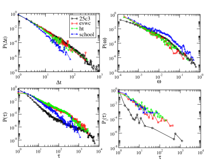
The heterogeneity and burstiness of the contact patterns of the face-to-face interactions Cattuto et al. (2010) are revealed by the study of the distribution of the duration of contacts between pairs of agents, , the distribution of the total time in contact of pairs of agents (the weight distribution ), and the distribution of gap times, , between two consecutive conversations involving a common individual and two other different agents, for a single agent , , or considering all the agents, . All these distributions are heavy-tailed, typically compatible with power-law behaviors (see Fig. 1), corresponding to the burstiness of human interactions Barabási (2005).
As noted above, diffusion processes such as random walks are moreover particularly impacted by the structure of paths between nodes. In this respect, time respecting paths represent a crucial feature of any temporal network, since they determine the set of possible causal interactions between the actors of the graph.
For each (ordered) pair of nodes , time-respecting paths from to can either exist or not; moreover, the concept of shortest path on static networks (i.e., the path with the minimum number of links between two nodes) yields several possible generalizations in a temporal network:
-
•
the fastest path is the one that allows to go from to , starting from the dataset initial time, in the minimum possible time, independently of the number of intermediate steps;
-
•
the shortest time-respecting path between and is the one that corresponds to the smallest number of intermediate steps, independently of the time spent between the start from and the arrival to .
For each node pair , we denote by , , the lengths (in terms of the number of hops) respectively of the fastest path, the shortest time-respecting path, and the shortest path on the aggregated network, and by and the duration of the fastest and shortest time-respecting paths, where we take as initial time the first appearance of in the dataset. As already noted in other works Kossinets et al. (2008); Isella et al. (2011), can be much larger than . Moreover, it is clear that ; from the duration point of view, on the contrary, .
We therefore define the following quantities:
-
•
: fraction of the ordered pairs of nodes for which a time-respecting path exists;
-
•
: average length (in terms of number of hops along network links) of the shortest time-respecting paths;
-
•
: average duration of the shortest time-respecting paths;
-
•
: average length of the fastest time-respecting paths;
-
•
: average duration of the fastest time-respecting paths;
-
•
: average shortest path length in the binary (static) projected network;
| Dataset | ||||||
|---|---|---|---|---|---|---|
| 25c3 | 0.91 | 1.67 | 1607 | 4.7 | 893 | 1.67 |
| eswc | 0.99 | 1.75 | 884 | 4.95 | 287 | 1.73 |
| ht | 0.99 | 1.67 | 1157 | 3.86 | 452 | 1.66 |
| school | 1 | 1.76 | 853 | 8.27 | 349 | 1.73 |
The corresponding empirical values are reported in Table 2. It turns out that the great majority of pairs of nodes are causally connected by at least one path in all datasets. Hence, almost every node can potentially be influenced by any other actor during the time evolution, i.e., the set of sources and the set of influence of the great majority of the elements are almost complete (of size ) in all of the considered datasets.
In Fig. 2 we show the distributions of the lengths, , and durations, , of the shortest time-respecting path for different datasets. In the same Figure we choose one dataset to compare the and the distributions with the distributions of the lengths, , and durations, , of the fastest path. The distribution is short tailed and peaked on , with a small average value , even considering the relatively small sizes of the datasets, and it is very similar to the projected network one (see Table 2). The distribution, on the contrary, shows a smooth behavior, with an average value several times bigger than the shortest path one, , as expected Kossinets et al. (2008); Isella et al. (2011). Note that, despite the important differences in the datasets characteristics, the distributions (as well as , although not shown) collapse, once rescaled. On the other hand, the and distributions show the same broad-tailed behavior, but the average duration of the shortest paths is much longer than the average duration of the fastest paths, and of the same order of magnitude than the total duration of the contact sequence .
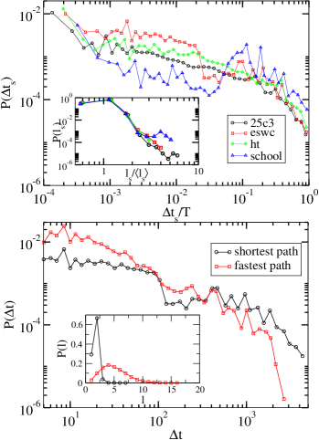
Thus, a temporal network may be topologically well connected and at the same time difficult to navigate or search. Indeed spreading and searching processes need to follow paths whose properties are determined by the temporal dynamics of the network, and that might be either very long or very slow.
III.3 Synthetic extensions of empirical contact sequences
The empirical contact sequences represent the proper dynamical network substrate upon which the properties of any dynamical process should be studied. In many cases however, the finite duration of empirical datasets is not sufficient to allow these processes to reach their asymptotic state Pan and Saramäki (2011); Stehlé et al. (2011a). This issue is particularly important in processes that reach a steady state, such as random walks. As discussed in Sec. II, a walker does not move at every time step, but only with a probability , and the effective number of movements of a walker is of the order . For the considered empirical sequences, this means that the ratio between the number of hops of the walker and the network size, , assumes values between for the school case and for the eswc case. Typically, for a random walk processes such small times permit to observe transient effects only, but not a stationary behavior. Therefore we will first explore the asymptotic properties of random walks in synthetically extended contact sequences, and we will consider the corresponding finite time effects in Sec. VI. The synthetic extensions preserve at different levels the statistical properties observed in the real data, thus providing null models of dynamical networks.
Inspired by previous approaches to the synthetic extension of empirical contact sequences Holme (2005); Pan and Saramäki (2011); Stehlé et al. (2011a); Kivela et al. (2011); Holme and Saramäki (2011), we consider the following procedures:
-
•
SRep: Sequence replication. The contact sequence is repeated periodically, defining a new extended characteristic function such that . This extension preserves all of the statistical properties of the empirical data (obviously, when properly rescaled to take into account the different durations of the extended and empirical time series), introducing only small corrections, at the topological level, on the distribution of time respecting paths and the associated sets of influence of each node. Indeed, a contact present at time will be again available to a dynamical process starting at time after a time .
-
•
SRan: Sequence randomization. The time ordering of the interactions is randomized, by constructing a new characteristic function such that, at each time step , and , where is a time chosen uniformly at random from the set . This form of extension yields at each time step an empirical instantaneous network of interactions, and preserves on average all the characteristics of the projected weighted network, but destroys the temporal correlations of successive contacts, leading to Poisson distributions for and .
-
•
SStat: Statistically extended sequence. An intermediate level of randomization can be achieved by generating a synthetic contact sequence as follows: we consider the set of all conversations in the sequence, defined as a series of consecutive contacts of length between the pair of agents and . The new sequence is generated, at each time step , by choosing conversations ( being the average number of new conversations starting at each time step in the original sequence, see Table 1), randomly selected from the set of conversations, and considering them as starting at time and ending at time , where is the duration of the corresponding conversation. In this procedure we avoid choosing conversations between agents and which are already engaged in a contact started at a previous time . This extension preserves all the statistical properties of the empirical contact sequence, with the exception of the distribution of time gaps between consecutive conversations of a single individual, .
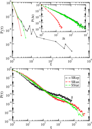
In Fig. 3 we plot the distribution of the duration of contacts, , and the distribution of gap times between two consecutive conversations realized by a single individual, , for the extended contact sequences SRep, SRan and SStat. One can check that the SRep extension preserves all the , and distributions of the original contact sequence, the SRan extension preserves only and the SStat extension preserves both the and the but not the , as summarized in Table 3. Interestingly, we note that the distribution of gap times for all agents, , is also broadly distributed in the SRan and SStat extensions, despite the fact that the respective individual burstiness are bounded, see Fig. 3. This fact can be easily understood by considering that can be written in terms of a convolution of the individual gap distributions times the probability of starting a conversation. In the case of SRan extension, the probability that an agent starts a new conversation is proportional to its strength , i.e. . Therefore, the probability that it starts a conversation time steps after the last one (its gap distribution) is given by , for sufficiently small . The gap distribution for all agents is thus given by the convolution
| (9) |
where is the strength distribution. This distribution has an exponential form, which leads, from Eq. (9), to a total gap distribution , with a heavy tail. Analogous arguments can be used in the case of the SStat extension.
| Extension | |||
|---|---|---|---|
| SRep | ✓ | ✓ | ✓ |
| SRan | ✓ | ✗ | ✗ |
| SStat | ✓ | ✓ | ✗ |
IV Random walks on extended contact sequences
Let us consider a random walk on the sequence of instantaneous networks at discrete time steps, which is equivalent to a message passing strategy in which the message is passed to a randomly chosen neighbor. The walker present at node at time hops to one of its neighbors, randomly chosen from the set of vertices
| (10) |
of which there is a number
| (11) |
If the node is isolated at time , i.e. , the walker remains at node . In any case, time is increased .
Analytical considerations analogous to those in Sec. II for the case of contact sequences are hampered by the presence of time correlations between contacts. In fact, as we have seen, the contacts between a given pair of agents are neither fixed nor completely random, but instead show long range temporal correlations. An exception is represented by the randomized SRan extension, in which successive contacts are by construction uncorrelated. Considering that the random walker is in vertex at time , at a subsequent time step it will be able to jump to a vertex whenever a connection between and is created, and a connection between and will be chosen with probability proportional to the number of connections between and in the original contact sequence, i.e. proportional to . That is, a random walk on the extended SRan sequence behaves essentially as in the corresponding weighted projected network, and therefore the equations obtained in Sec. II, namely
| (12) |
and
| (13) |
apply. In this last expression for the coverage we can approximate the sum by an integral, i.e.
| (14) |
being the distribution of strengths. Giving that has an exponential behavior, we can obtain from the last expression
| (15) |
V Numerical simulations
In this Section we present numerical results from the simulation of random walks on the extended contact sequences described above. Measuring the coverage we set the duration of these sequences to times the duration of the original contact sequence , while to evaluate the MFPT between two nodes and , , we let the RW explore the network up to a maximum time . Each result we report is averaged over at least independent runs.
V.1 Network exploration
The network coverage describes the fraction of nodes that the walker has discovered up to time . Figure 4 shows the normalized coverage as a function of time, averaged for different walks starting from different sources, for the dynamical networks obtained using the SRep, SRan and SStat prescriptions. Time is rescaled as to take into account that the walker can find itself on an isolated vertex, as discussed before. While for SRep and SRan extensions the average number of interacting nodes is by construction the same as in the original contact sequence, for the SStat extension we obtain numerically different values of , which we use when rescaling time in the corresponding simulations.
The coverage corresponding to the SRan extension is very well fitted by a numerical simulation of Eq. (15), which predicts the coverage obtained in the correspondent projected weighted network. Moreover, when using the rescaled time , the SRan coverages for different datasets collapse on top of each other for small times, with a linear time dependence for as expected in static networks, showing a universal behavior (not shown).
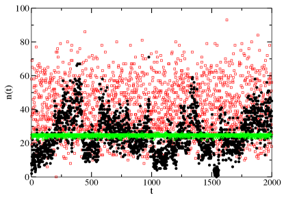
The coverage obtained on the SStat extension is systematically smaller than in the SRan case, but follows a similar evolution. On the other hand, the RW exploration obtained with the SRep prescription is generally slower than the other two, particularly for the 25c3 and ht datasets. As discussed before, the original contact sequence, as well as the SRep extension, are characterized by irregular distributions of the interactions in time, showing periods with few interacting nodes and correspondingly a small number of new started conversations, followed by peaks with many interactions (see Fig. 5). This feature slows down the RW exploration, because the RW may remain trapped for long times on isolated nodes. The SRan and the SStat extensions, on the contrary, both destroy this kind of temporal structure, balancing the periods of low and high activity: the SRan extension randomizes the time order of the contact sequence, and the SStat extension evens the number of interacting nodes, with new conversations starting at each time step.
The similarity between the random walk processes on the SRan and SStat dynamical networks shows that the random walk coverage is not very sensitive to the heterogenous durations of the conversations, as the main difference between these two cases is that is narrow for SRan and broad for SStat. In these cases, the observed behavior is instead well accounted for by Eq. (13), taking into account only the weight distribution of the projected network, i.e., the heterogeneity between aggregated conversation durations. Therefore, the slower exploration properties of the SRep sequences can be mostly attributed to the correlations between consecutive conversations of the single individuals, as given by the individual gap distribution , (see Stehlé et al. (2011a); Karsai et al. (2011); Kivela et al. (2011) for analogous results in the context of epidemic spreading).
A remark is in order for the 25c3 conference. A close inspection of Fig. 4 shows that the RW does not reach the whole network in any of the extensions schemes, with , although the duration of the simulation is quite long . The reason is that this dataset contains a group of nodes (around of the total) with a very low strength , meaning that there are actors who are isolated for most of the time, and whose interactions are reduced to one or two contacts in the whole contact sequence. Given that each extension we use preserves the distribution, the discovery of these nodes is very difficult. The consequence is that we observe an extremely slow approach to the asymptotic value . Indeed, the mean-field calculations presented in Secs. II and III.3 suggest a power-law decay with for the residual coverage .
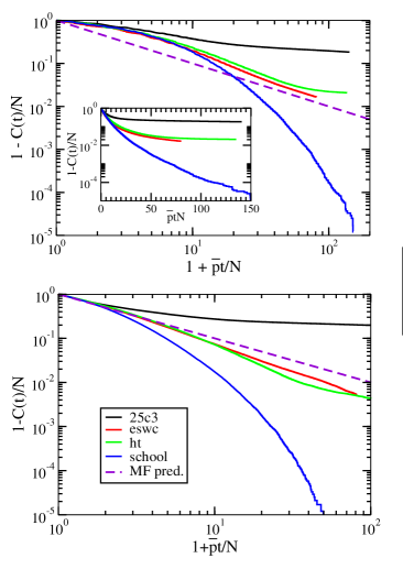
In Fig. 6 we plot the asymptotic coverage for large times in the 4 datasets considered. We can see that RW on the eswc and ht dataset conform at large times quite reasonably to the expected theoretical prediction in Eq. (15), both for the SRep and SRan extensions. The 25c3 dataset shows, as discussed above, a considerable slowing down, with a very slow decay in time. Interestingly, the school dataset is much faster than all the rest, with a decay of the residual coverage exhibiting an approximate exponential decay. It is noteworthy that the plots for the randomized SRan sequence do not always obey the mean-field prediction (see lower plot in Fig. 6). This deviation can be attributed to the fact that SRan extensions preserve the topological structure of the projected weighted network, and it is known that, in some instances, random walks on weighted networks can deviate from the mean-field predictions Baronchelli and Pastor-Satorras (2010). These deviations are particularly strong in the case of the 25c3 dataset, where connections with a very small weight are present.
V.2 Mean first-passage time
Let us now focus on another important characteristic property of random walk processes, namely the MFPT defined in Section II. Figure 7 shows the correlation between the MFPT of each node, measured in units of rescaled time , and its normalized strength .
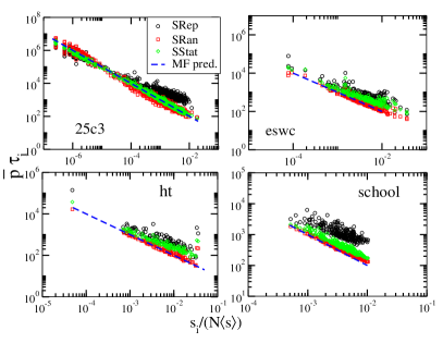
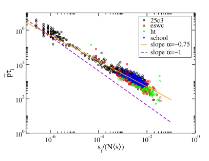
The random walks performed on the SRan and SStat extensions are very well fitted by the mean field theory, i.e. Eq. (12) (predicting that is inversely proportional to ), for every dataset considered; on the other hand, random walks on the extended sequence SRep yield at the same time deviations from the mean-field prediction and much stronger fluctuations around an average behavior. Figure 8 addresses this case in more detail, showing that the data corresponding to RW on different datasets collapse on an average behavior that can be fitted by a scaling function of the form
| (16) |
with an exponent .
These results show that the MFPT, similarly to the coverage, is rather insensitive to the distribution of the contact durations, as long as the distribution of cumulated contact durations between individuals is preserved (the weights of the links in the projected network). Therefore, the deviations of the results obtained with the SRep extension of the empirical sequences have their origin in the burstiness of the contact patterns, as determined by the temporal correlations between consecutive conversations. The exponent means that the searching process in the empirical, correlated, network is slower than in the randomized versions, in agreement with the smaller coverage observed in Fig. 4.
The data collapse observed in Fig. 8 for the SRep case leads to two noticeable conclusions. First, although the various datasets studied correspond to different contexts, with different numbers of individuals and densities of contacts, simple rescaling procedures are enough to compare the processes occurring on the different temporal networks, at least for some given quantities. Second, the MFPT at a node is largely determined by its strength. This can indeed seem counterintuitive as the strength is an aggregated quantity (that may include contact events occurring at late times). However, it can be rationalized by observing that a large strength means a large number of contacts and therefore a large probability to be reached by the random walker. Moreover, the fact that the strength of a node is an aggregate view of contact events that do not occur homogeneously for all nodes but in a bursty fashion leads to strong fluctuations around the average behavior, which implies that nodes with the same strength can also have rather different MFPT (Note the logarithmic scale on the y-axis).
VI Random walks on finite contact sequences
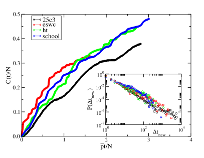
The case of finite sequences is interesting from the point of view of realistic searching processes. The limited duration of a human gathering, for example, imposes a constraint on the length of any searching strategy. Fig. 9 shows the normalized coverage as a function of the rescaled time . The coverage exhibits a considerable variability in the different datasets, which do not obey the rescaling obtained for the extended SRan and SStat sequence. The probability distribution of the time lags between the discovery of two new vertices Baronchelli et al. (2008) provides further evidence of the slowing down of diffusion in temporal networks. The inset of Fig. 9 indeed shows broad tailed distributions for all the dataset considered, differently from the exponential decay observed in binary static networks Baronchelli et al. (2008).
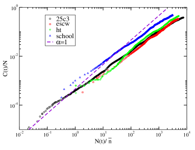
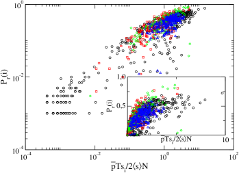
The important differences in the rescaled coverage between the various datasets, shown in Fig. 9, can be attributed to the choice of the time scale, , which corresponds to a temporal rescaling by an average quantity. We can argue, indeed, that the speed with which new nodes are found by the RW is proportional to the number of new conversations started at each time step , thus in the RW exploration of the temporal network the effective time scale is given by the integrated number of new conversations up to time , . In Fig. 10 we display the correlation between the coverage and the number of new conversations realized up to time , , normalized for the mean number of new conversations per unit of time, . While the relation is not strictly linear, a very strong positive correlation appears between the two quantities.
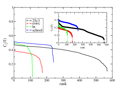
The complex pattern shown by the average coverage originates from the lack of self-averaging in a dynamic network. Figure 11 shows the rank plot of the coverage obtained at the end of a RW process starting from node , and averaged over runs. Clearly, not all vertices are equivalent. A first explanation of the variability in comes from the fact that not all nodes appear simultaneously on the network at time . If denotes the arrival time of node in the system, a random walk starting from is restricted to : nodes arriving at later times have less possibilities to explore their set of influence, even if this set includes all nodes. To put all nodes on equal footing and compensate for this somehow trivial difference between nodes, we consider the coverage of random walkers starting on the different vertices and walking for exactly time steps (we limit of course the study to nodes with ). Differences in the coverage will then depend on the intrinsic properties of the dynamic network. For a static network indeed, either binary or weighted, the coverage would be independent of , as random walkers on static networks lose the memory of their initial position in a few steps, reaching very fast the steady state behavior Eq. (3). As the inset of Fig. 11 shows, important heterogeneities are instead observed in the coverage of random walkers starting from different nodes on the dynamic network, even if the random walk duration is the same.
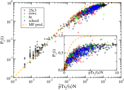
Another interesting quantity is the probability that a vertex is discovered by the random walker. As discussed in Section II, at the mean field level the probability that a node is visited by the RW at any time less than or equal to (the random walk reachability) takes the form . Thus the probability that the node is reached by the RW at any time in the contact sequence is
| (17) |
where the rescaled time is taken into account. In Fig. 12, we plot the probability of node to be reached by the RW during the contact sequence as a function of its strength . exhibits a clear increasing behavior with , larger strength corresponding to larger time in contact and therefore larger probabilities to be reached. Interestingly, the simple rescaling by and leads to an approximate data collapse for the RW processes on the various dynamical networks, showing a very robust behavior. Similarly to the case of the MFPT on extended sequences, the dynamical property can be in part “predicted” by an aggregate quantity such as . Strong deviations from the mean-field prediction of Eq. (17) are however observed, with a tendency of to saturate at large strengths to values much smaller than the ones obtained on a static network. Thus, although the set of sources of almost every node has size , as shown in Sec. III.2 (i.e., there exists a time respecting path between almost every possible starting point of the RW processes and every target node ), the probability for node to be effectively reached by a RW is far from being equal to .
Moreover, rather strong fluctuations of at given are also observed: is indeed an aggregate view of contacts which are typically inhomogeneous in time, with bursty behaviors222When considering RW on a contact sequence of length randomized according to the SRan procedure instead, Eq. (17) is well obeyed and only small fluctuations of are observed at a fixed (not shown). . Figure 13 also shows that the reachability computed at shorter time (here ) displays stronger fluctuations as a function of the strength computed on the whole time sequence: for shorter RW is naturally less correlated with an aggregate view which takes into account a more global behavior of .
VII Discussion and conclusions
In this paper we have investigated the behavior of random walks on temporal networks. In particular, we have focused on real face-to-face contact networks concerning four different datasets. These dynamical networks exhibit heterogeneous and bursty behavior, indicated by the long tailed distributions for the lengths and strength of conversations, as well as for the gaps separating successive interactions. We have underlined the importance of considering not only the existence of time preserving paths between pairs of nodes, but also their temporal duration: shortest paths can take much longer than fastest paths, while fastest paths can correspond to many more hops than shortest paths. Interestingly, the appropriate rescaling of these quantities identifies universal behaviors shared across the four datasets.
Given the finite life-time of each network, we have considered as substrate for the random walk process the replicated sequences in which the same time series of contact patterns is indefinitely repeated. At the same time, we have proposed two different randomization procedures to investigate the effects of correlations in the real dataset. The “sequence randomization” (SRan) destroys any temporal correlation by randomizing the time ordering of the sequence. This allows to write down exact mean-field equations for the random walker exploring these networks, which turn out to be substantially equivalent to the ones describing the exploration of the weighted projected network. The “statistically extended sequence” (SStat), on the other hand, selects random conversations from the original sequence, thus preserving the statistical properties of the original time series, with the exception of the distribution of time gaps between consecutive conversations.
We have performed numerical analysis both for the coverage and the MFPT properties of the random walker. In both cases we have found that the empirical sequences deviate systematically from the mean field prediction, inducing a slowing down of the network exploration and of the MFPT. Remarkably, the analysis of the randomized sequences has allowed us to point out that this is due uniquely to the temporal correlations between consecutive conversations present in the data, and not to the heterogeneity of their lengths. Finally, we have addressed the role of the finite size of the empirical networks, which turns out to prevent a full exploration of the random walker, though differences exist across the four considered cases. In this context, we have also shown that different starting nodes provide on average different coverages of the networks, at odds to what happens in static graphs. In the same way, the probability that the node is reached by the RW at any time in the contact sequence exhibits a common behavior across the different time series, but it is not described by the mean-field predictions for the aggregated network, which predict a faster process.
In conclusion, the contribution of our analysis is two-fold. On the one hand, we have proposed a general way to study dynamical processes on temporally evolving networks, by the introduction of randomized benchmarks and the definition of appropriate quantities that characterize the network dynamics. On the other hand, for the specific, yet fundamental, case of the random walk, we have obtained detailed results that clarify the observed dynamics, and that will represent a reference for the understanding of more complex diffusive dynamics occurring on dynamic networks. Our investigations also open interesting directions for future work. For instance, it would be interesting to investigate how random walks starting from different nodes explore first their own neighborhood Baronchelli and Loreto (2006), which might lead to hints about the definition of “temporal communities” (see e.g. Pons and Latapy (2005) for an algorithm using RW on static networks for the detection of static communities); various measures of nodes centrality have also been defined in temporal networks Braha and Bar-Yam (2009); Tang et al. (2010b); Lerman et al. (2010); Pan and Saramäki (2011); Holme and Saramäki (2011), but their computation is rather heavy, and RW processes might present interesting alternatives, similarly to the case of static networks Newman (2005).
Acknowledgments
We thank the SocioPatterns collaboration (www.sociopatterns.org) for providing privileged access to dynamical network data. M.S., R.P.-S. and A. Baronchelli acknowledge financial support from the Spanish MEC (FEDER), under project FIS2010-21781-C02-01, and the Junta de Andalucía, under project No. P09-FQM4682.. R.P.-S. acknowledges additional support through ICREA Academia, funded by the Generalitat de Catalunya.
References
- Holme and Saramäki (2011) P. Holme and J. Saramäki, “Temporal networks,” (2011), eprint arxiv:1108.1780v1 .
- Wasserman and Faust (1994) S. Wasserman and K. Faust, Social Network Analysis: Methods and Applications (Cambridge University Press, Cambridge, 1994).
- Newman (2001) M. E. J. Newman, Proc. Natl. Acad. Sci. USA 98, 404 (2001).
- Barabási and Albert (1999) A.-L. Barabási and R. Albert, Science 286, 509 (1999).
- Barrat et al. (2008) A. Barrat, M. Barthélemy, and A. Vespignani, Dynamical processes on complex networks (Cambridge, 2008).
- Hui et al. (2005) P. Hui, A. Chaintreau, J. Scott, R. Gass, J. Crowcroft, and C. Diot, in WDTN ’05: Proceedings of the 2005 ACM SIGCOMM workshop on Delay-tolerant networking (ACM, New York, NY, USA, 2005) pp. 244–251.
- Holme (2005) P. Holme, Phys. Rev. E 71, 046119 (2005).
- Onnela et al. (2007) J.-P. Onnela, J. Saramäki, J. Hyvönen, G. Szabó, D. Lazer, K. Kaski, J. Kertész, and A.-L. Barabási, Proceedings of the National Academy of Sciences 104, 7332 (2007).
- Gautreau et al. (2009) A. Gautreau, A. Barrat, and M. Barthélemy, Proceedings of the National Academy of Sciences 106, 8847 (2009).
- Cattuto et al. (2010) C. Cattuto, W. Van den Broeck, A. Barrat, V. Colizza, J.-F. Pinton, and A. Vespignani, PLoS ONE 5, e11596 (2010).
- Tang et al. (2010a) J. Tang, S. Scellato, M. Musolesi, C. Mascolo, and V. Latora, Phys. Rev. E 81, 055101 (2010a).
- Bajardi et al. (2011) P. Bajardi, A. Barrat, F. Natale, L. Savini, and V. Colizza, PLoS ONE 6, e19869 (2011).
- Stehlé et al. (2011a) J. Stehlé, N. Voirin, A. Barrat, C. Cattuto, V. Colizza, L. Isella, C. Régis, J.-F. Pinton, N. Khanafer, W. Van den Broeck, and P. Vanhems, BMC Medicine 9 (2011a).
- Miritello et al. (2011) G. Miritello, E. Moro, and R. Lara, Phys. Rev. E 83, 045102 (2011).
- Karsai et al. (2011) M. Karsai, M. Kivelä, R. K. Pan, K. Kaski, J. Kertész, A.-L. Barabási, and J. Saramäki, Phys. Rev. E 83, 025102 (2011).
- Scherrer et al. (2008) A. Scherrer, P. Borgnat, E. Fleury, J.-L. Guillaume, and C. Robardet, Comp. Net. 52, 2842 (2008).
- Hill and Braha (2010) S. Hill and D. Braha, Phys. Rev. E 82, 046105 (2010).
- Stehlé et al. (2010) J. Stehlé, A. Barrat, and G. Bianconi, Phys. Rev. E 81, 035101 (2010).
- Zhao et al. (2011) K. Zhao, J. Stehlé, G. Bianconi, and A. Barrat, Phys. Rev. E 83, 056109 (2011).
- Rocha et al. (2011) L. E. C. Rocha, F. Liljeros, and P. Holme, PLoS Comput Biol 7, e1001109 (2011).
- Isella et al. (2011) L. Isella, J. Stehlé, A. Barrat, C. Cattuto, J.-F. Pinton, and W. V. den Broeck, J. Theor. Biol 271, 166 (2011).
- Kivela et al. (2011) M. Kivela, R. Kumar Pan, K. Kaski, J. Kertesz, J. Saramaki, and M. Karsai, “Multiscale analysis of spreading in a large communication network,” (2011), arXiv:1112.4312v1.
- Fujiwara et al. (2011) N. Fujiwara, J. Kurths, and A. Díaz-Guilera, Physical Review E 83, 025101 (2011).
- Parshani et al. (2010) R. Parshani, M. Dickison, R. Cohen, H. E. Stanley, and S. Havlin, EPL (Europhysics Letters) 90, 38004 (2010).
- Baronchelli and Díaz-Guilera (2012) A. Baronchelli and A. Díaz-Guilera, Phys. Rev. E 85, 016113 (2012).
- Weiss (1994) G. H. Weiss, Aspects and Applications of the Random Walk (North-Holland Publishing Co., Amsterdam, 1994).
- Hughes (1995) B. Hughes, Random walks and random environments (Clarendon Press, Oxford (UK), 1995).
- Lovász (1996) L. Lovász, in Combinatorics, Paul Erdös is Eighty (János Bolyai Mathematical Society, Budapest, 1996) p. 353.
- Adamic et al. (2001) L. A. Adamic, R. M. Lukose, A. R. Puniyani, and B. A. Huberman, Phys. Rev. E 64, 046135 (2001).
- Lv et al. (2002) Q. Lv, P. Cao, E. Cohen, K. Li, and S. Shenker, in Proceedings of the 16th international conference on Supercomputing (ACM Press, New York, NY, USA, 2002) pp. 84–95.
- (31) http://www.sociopatterns.org/.
- Barrat et al. (2004) A. Barrat, M. Barthélemy, R. Pastor-Satorras, and A. Vespignani, Proc. Natl. Acad. Sci. USA 101, 3747 (2004).
- Noh and Rieger (2004) J. D. Noh and H. Rieger, Phys. Rev. Lett. 92, 118701 (2004).
- Wu et al. (2007) A.-C. Wu, X.-J. Xu, Z.-X. Wu, and Y.-H. Wang, Chin. Phys. Lett. 24, 577 (2007).
- Stauffer and Sahimi (2005) D. Stauffer and M. Sahimi, Phys. Rev. E 72, 46128 (2005).
- Almaas et al. (2003) E. Almaas, R. V. Kulkarni, and Stroud, Phys. Rev. E 68, 056105 (2003).
- Newman (2010) M. E. J. Newman, Networks: An introduction (Oxford University Press, Oxford, 2010).
- Stehlé et al. (2011b) J. Stehlé, N. Voirin, A. Barrat, C. Cattuto, L. Isella, J.-F. Pinton, M. Quaggiotto, W. Van den Broeck, C. Régis, B. Lina, and P. Vanhems, PLoS ONE 6, e23176 (2011b).
- Kostakos (2009) V. Kostakos, Physica A: Statistical Mechanics and its Applications 388, 1007 (2009).
- Nicosia et al. (2011) V. Nicosia, J. Tang, M. Musolesi, G. Russo, C. Mascolo, and V. Latora, arXiv:1106.2134 (2011).
- Barabási (2005) A. Barabási, Nature 435, 207 (2005).
- den Broeck et al. (2010) W. V. den Broeck, C. Cattuto, A. Barrat, M. Szomsor, G. Correndo, and H. Alani, in Proceedings of the 8th Annual IEEE International Conference on Pervasive Computing and Communications (2010) p. 226.
- Kossinets et al. (2008) G. Kossinets, J. Kleinberg, and D. Watts, in Proceedings of the 14 ACM SIGKDD International Conference on Knowledge Discovery and Data Mining (2008).
- Pan and Saramäki (2011) R. K. Pan and J. Saramäki, Phys. Rev. E 84, 016105 (2011).
- Baronchelli and Pastor-Satorras (2010) A. Baronchelli and R. Pastor-Satorras, Phys. Rev. E 82, 011111 (2010).
- Baronchelli et al. (2008) A. Baronchelli, M. Catanzaro, and R. Pastor-Satorras, Phys. Rev. E 78, 011114 (2008).
- Baronchelli and Loreto (2006) A. Baronchelli and V. Loreto, Phys. Rev. E 73, 026103 (2006).
- Pons and Latapy (2005) P. Pons and M. Latapy, in Proceedings of the 20th International Symposium on Computer and Information Sciences (ISCIS’05), Lecture Notes in Computer Science, Vol. 3733 (Springer, Istanbul, Turkey, 2005) pp. 284–293.
- Braha and Bar-Yam (2009) D. Braha and Y. Bar-Yam, in Adaptive Networks, Understanding Complex Systems, Vol. 51, edited by T. Gross and H. Sayama (Springer Berlin / Heidelberg, 2009) pp. 39–50.
- Tang et al. (2010b) J. Tang, M. Musolesi, C. Mascolo, V. Latora, and V. Nicosia, in Proceedings of the 3rd Workshop on Social Network Systems, SNS ’10 (ACM, New York, NY, USA, 2010) pp. 3:1–3:6.
- Lerman et al. (2010) K. Lerman, R. Ghosh, and J. H. Kang, in Proceedings of the Eighth Workshop on Mining and Learning with Graphs, MLG ’10 (ACM, New York, NY, USA, 2010) pp. 70–77.
- Newman (2005) M. J. Newman, Social Networks 27, 39 (2005).