Can quantum mechanics be considered as statistical? an analysis of the PBR theorem

Abstract

The answer to this question is ‘yes it can!’ as we will see in this manuscript. More, precisely after a discussion of M. F. Pusey, J. Barrett and T. Rudolph (PBR) result (arXiv:1111.3328) we will show that contrarily to the PBR claim the epistemic approach is in general not disproved by their ‘no-go’ theorem.

I A $\Psi$-losophical introduction

I.1 Liouville’s realm

Classical physics which is based on physical realism makes the distinction between ontic and epistemic state in a clean way. The ‘ontic’ state are the actual values of the dynamical variables $q(t),p(t)$ defined in the evolution or configuration space and solutions of the Hamilton or Lagrange equations describing the system. They represent the system even if there is not observer at least in a local universe (for a nonlocal universe where correlations can exist between disconnected region of space and time the definition should probably be amended a bit: one could for example states that the absence or presence of the observer should not disturb ‘too much’ the rest of the universe). The inclusion of the observer involves others dynamical variables $Q(t),P(t)$ (therefore the observer is included in the theory). In principle, the coupling between the observer and the system of interest could be reduced at will and therefore the ontic state is also experimentally accessible. The ‘epistemic’ state is the density of probability $\rho(q,p,t)$ defined in the same configuration space and which evolves in time following the Liouville equation $d\rho(q(t),p(t),t)/dt=\partial\rho/\partial t+\{\rho,H\}=0$. It represents the objective-subjective knowledge of the experimenter and is statistic by nature (of course certainty is a particular degenerate case of this general frame). In classical physics the density being given at one time $t_{0}$ one can calculate it at any times (past or future). Additionally, we can arbitrary ‘mathematically’ impose $\rho(t_{0})$ in the equations. Fundamentally, this means that the dynamic is decoupled from the probabilistic evolution: the trajectories in the evolution space are the same whatever the density function $\rho$ chosen. This is an important property which in part explains why the statistical mechanics of Boltzmann-Gibbs requires some additional postulates (based on symmetries or plausible boundary conditions in the remote past) in order to fix the equilibrium states of statistical thermodynamics. The foundations of statistical physics is still a subject of active research (in particular if we consider the subjective-objective dualism concerning interpretation of probability). However, its foundation relying on an ontic state $q(t),p(t)$ is universally accepted by classical physicist and therefore never contradicts realism.

I.2 Heisenberg’s realm

In quantum mechanics the situation is different. Indeed, we start from a statistical theory ‘the epistemic state’ but we don’t have any dynamic or trajectory $q(t),p(t)$. Instead, we have observable $Q,P$ which can not all be measured ‘simultaneously’ for the same individual system. This leads to the principle of complementarity which states that measurement associated with non commuting operator require experimental procedures which mutually exclude each other. In the same vain by a generalization of Heisenberg uncertainty principle we deduce that due to entanglement, i.e. quantum correlation, with the measurement apparatus we cannot define unambiguously et univocally the hypothetical ‘classical’ path followed by a particle in an interferometer. Therefore, the wave-particle dualism cannot be solved experimentally and the concept of trajectories become somehow metaphysical. The introduction of hidden dynamical variables written generically $\lambda(t)$ after Bell is therefore regarded by most orthodox quantum practitioners as a kind of useless superstructure identical by nature to the hypothetical Ether postulated in the XIX^th century. However, postulating the mere existence of such $\lambda(t)$ has at least the advantage to solve the problem of the ‘Heisenberg-cut’ that is the duality classic-quantum or observer-object which is so important in Bohr philosophy. In the Copenhagen interpretation we must indeed accept a form a macro realism (with all what this implies) together with a micro ‘non-realism’ (whatever this can mean). However, since the cut is movable it is difficult to understand how realism can mute into non-realism or reciprocally (the ‘cut’ leads even to uncountable difficulties if we consider seriously Einstein’s relativity and its arbitresses concerning space-time foliations and reference frames). Clearly, if we accept the hidden variable approach the problem is automatically solved in a simple and drastic way since then the paradoxical cut does not exist anymore (I think that it was also the point stressed by Schrodinger in its famous cat example). I am not sure that practitioners of orthodox quantum mechanics would really appreciate this fact. For them the counter intuitive nature of such $\lambda$-theories (in particular after Bell theorem concerning nonlocality in the 1960’s) would make the price too high to pay and they would probably prefer to let the question open or at least not decidable. I would even say than in order to convince quantum mechanics practitioners one or more revolutionary principles are clearly missing to solve the problem of nonlocality in a not ad-hoc way. Additionally, such a model should ultimately make new predictions going beyond current quantum mechanics (again the problem of Ether).
Still, for the present days it is at least on a logical ground remarkable that hidden variable models can be precisely defined. It was indeed in my opinion the clear merit of de Broglie and Bohm to construct such a hidden variable model (the only one which is working fine for all practical purpose i.e. without modifying Schrodinger equation I would even say). The model is classical in the ontic sense discussed before since it introduces trajectories but it is also epistemic since it reproduces every statistical predictions of standard quantum mechanics through a clearly (unfortunately) nonlocal and contextual dynamic. For this last reason it would be better to call the model neo-classic since there is no nonlocal interaction in classical XIX^th century physics.
After Bell’s work people get more interested in this topic and in Bohm’s work since they discovered that they can put some experimental limits on the apriori infinite number of possible $\lambda$-theories by using some ‘simple’ no-go theorems. In particular, local causal models can be eliminated if we reject loopholes, fatalistic and superdeterministic approaches. By the same approach non-contextuality was also eliminated by Bell, Kochen and Specker (BKS).

I.3 New no-go games?

Recently, a new work by M. Pusey, J. Barret and T. Rudolph (PBR in the following) was put on arxiv PBR and submitted for publication claiming a new revolutionary no-go theorem. This of course stirred much debates in blog discussions (see for example the blog of M. Leifer: http://mattleifer.info/ from which I stole the title of the present text) and Nature even posted an article about it. The idea of the PBR theorem will be discussed in details below but shortly its aim can be summarized in a simple way. Indeed, PBR show that if a hidden variable exists it can not be epistemic in a specifical sense of the word epistemic. More precisely, the theorem (which is I think mathematically true) states that the only way to include hidden variable in a description of the quantum world is to suppose that for every pair of quantum states $\Psi_{1}$ and $\Psi_{2}$ the density of probability must satisfy the condition of non intersecting support in the $\lambda$-space:

$$\rho(\lambda,\Psi_{1})\rho(\lambda,\Psi_{2})=0 \forall\lambda.$$ (1)

If this theorem is true it would really make hidden variables redundant (as I perceived it) since it could be possible to define a bijection or relation of equivalence between the lambda space and the Hilbert space: (loosely speaking we could in principle make the correspondence $\lambda\Leftrightarrow\psi$). Therefore it would be as if $\lambda$ is nothing that a new name for $\Psi$ it self (not even an Ether).
Very recently I read the PBR paper with a lot of interest in particular because I had the feeling that they missed something. I will try in the following to show what they missed and what it means really for hidden variable theories. At the end I hope that I will manage to convince you that it is still possible to deny the validity of Eq. 1 for most interesting $\lambda$-models.

II The PBR theorem

II.1 orthogonal states

We consider a simple Q-bit space $\mathbb{E}$ and two states $|\Psi_{1}\rangle$ and $|\Psi_{2}\rangle$ such that in the orthogonal basis $|\pm\rangle$ we have

$$\langle+|\Psi_{1}\rangle=\langle-|\Psi_{2}\rangle=0.$$ (2)

Clearly the states are orthogonal since

$$\langle\Psi_{2}|\Psi_{1}\rangle=\langle\Psi_{2}|[|+\rangle\langle+|+|-\rangle\langle-|]\Psi_{1}\rangle$$

$$=\langle\Psi_{2}|+\rangle\langle+|-\rangle\langle-|\Psi_{1}\rangle=0.$$ (3)

We now consider a hidden variable model and we write the probabilities to find the outcomes $\pm$

$$|\langle+|\Psi_{1}\rangle|^{2}=P(+|\Psi_{1})=\int\xi(+|\lambda)\rho_{1}(\lambda)d\lambda=0$$

$$|\langle-|\Psi_{2}\rangle|^{2}=P(-|\Psi_{2})=\int\xi(-|\lambda)\rho_{2}(\lambda)d\lambda=0.$$ (4)

In these equations we introduced the conditional ‘transition’ probabilities $\xi(\alpha|\lambda)$ for the outcomes $\alpha=\pm 1$ supposing given the hidden state $\lambda$. We have of course $\xi(+|\lambda)+\xi(-|\lambda)=1$. For the case here considered we deduce $\xi(+|\lambda)=0$ if $\rho_{1}(\lambda)\neq 0$ and similarly $\xi(-|\lambda)=0$ if $\rho_{2}(\lambda)\neq 0$.
We then obtain that if $\rho_{2}(\lambda)\cdot\rho_{1}(\lambda)\neq 0$ for some values of $\lambda$ (which means that $\rho_{1}$ and $\rho_{2}$ have intersecting supports in the $\lambda$-space ) then $\xi(+|\lambda)=\xi(-|\lambda)=0$ for such $\lambda$ values. Now this is impossible since we have by definition $\xi(+|\lambda)+\xi(-|\lambda)=1$ for every $\lambda$. We conclude therefore that $\rho_{2}(\lambda)\cdot\rho_{1}(\lambda)=0$ for every $\lambda$ i.e. that $\rho_{1}$ and $\rho_{2}$ have nonintersecting supports in the $\lambda$-space.

II.2 non-orthogonal states

We consider in the same Q-bit space the two states $|\Psi_{1}\rangle$ and $|\Psi_{2}\rangle$ defined by

$$|\Psi_{1}\rangle=|0\rangle, \textrm{and }|\Psi_{2}\rangle=|+\rangle$$ (5)

where $|0\rangle$ and $|1\rangle$ is an orthogonal basis and where $|\pm\rangle=\frac{1}{\sqrt{2}}[|0\rangle\pm|1\rangle]$ is a second orthogonal basis.
Now we introduce the 2 Q-bit Hilbert space $\mathbb{E}\otimes\mathbb{E}$ and the orthogonal basis

$$|\Phi_{1}\rangle=\frac{1}{\sqrt{2}}[|0\rangle\otimes|1\rangle+|1\rangle\otimes|0\rangle]$$

$$|\Phi_{2}\rangle=\frac{1}{\sqrt{2}}[|0\rangle\otimes|-\rangle+|1\rangle\otimes|+\rangle]$$

$$|\Phi_{3}\rangle=\frac{1}{\sqrt{2}}[|+\rangle\otimes|1\rangle+|-\rangle\otimes|0\rangle]$$

$$|\Phi_{4}\rangle=\frac{1}{\sqrt{2}}[|+\rangle\otimes|-\rangle+|-\rangle\otimes|+\rangle]$$ (6)

We are interested in the four states $|\Psi_{1}\rangle\otimes|\Psi_{1}\rangle$, $|\Psi_{1}\rangle\otimes|\Psi_{2}\rangle$, $|\Psi_{2}\rangle\otimes|\Psi_{1}\rangle$, and $|\Psi_{2}\rangle\otimes|\Psi_{2}\rangle$. We get the following coefficient matrix in the $\Phi$ basis:

	$|\Phi_{1}\rangle$	$|\Phi_{2}\rangle$	$|\Phi_{3}\rangle$	$|\Phi_{4}\rangle$
$|\Psi_{1}\rangle\otimes|\Psi_{1}\rangle$	0	$1/2$	$1/2$	$1/\sqrt{2}$
$|\Psi_{1}\rangle\otimes|\Psi_{2}\rangle$	$1/2$	0	$1/\sqrt{2}$	$1/2$
$|\Psi_{2}\rangle\otimes|\Psi_{1}\rangle$	$1/2$	$1/\sqrt{2}$	0	$1/2$
$|\Psi_{2}\rangle\otimes|\Psi_{2}\rangle$	$1/\sqrt{2}$	$1/2$	$1/2$	0

Table 1: Coefficient table in the $\Phi$ basis.

We now introduce a hidden variable model and we write the probabilities $P(\Phi_{i}|\Psi_{j}\otimes\Psi_{k})=|\langle\Phi_{i}|\Psi_{j}\otimes\Psi_{k}\rangle|^{2}$ as

$$P(\Phi_{i}|\Psi_{j}\otimes\Psi_{k})=\int\int\xi(\Phi_{i}|\lambda,\lambda^{\prime})\rho_{j}(\lambda)\rho_{k}(\lambda^{\prime})d\lambda d\lambda^{\prime}$$ (7)

where $i=[1,2,3,4]$ and $j,k=[1,2]$. In this PBR model there is a independence criteria at the preparation since we write $\rho_{j,k}(\lambda,\lambda^{\prime})=\rho_{j}(\lambda)\rho_{k}(\lambda^{\prime})$. The measurement is however obviously non local from the form of $\Phi_{i}$.
Now, clearly from the table we get:

$$P(\Phi_{1}|\Psi_{1}\otimes\Psi_{1})=\int\int\xi(\Phi_{1}|\lambda,\lambda^{\prime})\rho_{1}(\lambda)\rho_{1}(\lambda^{\prime})d\lambda d\lambda^{\prime}=0$$

$$P(\Phi_{2}|\Psi_{1}\otimes\Psi_{2})=\int\int\xi(\Phi_{2}|\lambda,\lambda^{\prime})\rho_{1}(\lambda)\rho_{2}(\lambda^{\prime})d\lambda d\lambda^{\prime}=0$$

$$P(\Phi_{3}|\Psi_{2}\otimes\Psi_{1})=\int\int\xi(\Phi_{3}|\lambda,\lambda^{\prime})\rho_{2}(\lambda)\rho_{1}(\lambda^{\prime})d\lambda d\lambda^{\prime}=0$$

$$P(\Phi_{4}|\Psi_{2}\otimes\Psi_{2})=\int\int\xi(\Phi_{4}|\lambda,\lambda^{\prime})\rho_{2}(\lambda)\rho_{2}(\lambda^{\prime})d\lambda d\lambda^{\prime}=0.$$

The first line implies $\xi(\Phi_{1}|\lambda,\lambda^{\prime})=0$ if $\rho_{1}(\lambda)\rho_{1}(\lambda^{\prime})\neq 0$. This condition is always satisfied if $\lambda$ and $\lambda^{\prime}$ are in the support of $\rho_{1}$ in the $\lambda$-space and $\lambda^{\prime}$-space. Similarly the fourth line implies $\xi(\Phi_{4}|\lambda,\lambda^{\prime})=0$ if $\rho_{2}(\lambda)\rho_{2}(\lambda^{\prime})\neq 0$ which is again always satisfied if $\lambda$ and $\lambda^{\prime}$ are in the support of $\rho_{2}$ in the $\lambda$-space and $\lambda^{\prime}$-space.
Finally the second and third lines imply $\xi(\Phi_{2}|\lambda,\lambda^{\prime})=0$ respectively $\xi(\Phi_{3}|\lambda,\lambda^{\prime})=0$ if $\rho_{1}(\lambda)\rho_{2}(\lambda^{\prime})\neq 0$ respectively $\rho_{1}(\lambda)\rho_{2}(\lambda^{\prime})\neq 0$. Taken separately these four conditions are not problematic. However in order to be true simultaneously and then to have

$$\xi(\Phi_{1}|\lambda,\lambda^{\prime})=\xi(\Phi_{2}|\lambda,\lambda^{\prime})=\xi(\Phi_{3}|\lambda,\lambda^{\prime})=\xi(\Phi_{4}|\lambda,\lambda^{\prime})=0$$

(9)

for a same pair of $\lambda,\lambda^{\prime}$ the conditions require that the supports of $\rho_{1}$ and $\rho_{2}$ intersect. If this is the case Eq. 9 will be true for any pair $\lambda,\lambda^{\prime}$ in the intersection.
However, this is impossible since we must have $\sum_{i=1}^{i=4}\xi(\Phi_{i}|\lambda,\lambda^{\prime})=1$ for every pair $\lambda,\lambda^{\prime}$. We conclude that $\rho_{1}(\lambda)\rho_{2}(\lambda)=0$ i.e. the supports of $\rho_{1}$ and $\rho_{2}$ are disjoints.
The result is not yet completely general since we studied only two particular states of $\mathbb{E}$. In order to generalize this result PBR considered the pair of non orthogonal states $|0\rangle$, $|0\rangle+\tan(\theta)e^{i\chi}|1\rangle$ (with $0<\theta<\pi/2$ and $\chi$ a phase). Using a basis rotation by an angle $\theta/2$ and absorbing the phase $\chi$ in the basis definition this pair of states can be re-parameterized as $|\psi_{0}\rangle=\cos{(\theta/2)}|0\rangle-\sin{(\theta/2)}|1\rangle$, $|\psi_{1}\rangle=\cos{(\theta/2)}|0\rangle+\sin{(\theta/2)}|1\rangle$.
Next PBR considered the n-uplet states $|\Psi(x_{1},...,x_{n})\rangle$ in the nQ-bits space $\mathbb{E}\otimes...\otimes\mathbb{E}$ and defined as

$$|\Psi(x_{1},...,x_{n})\rangle=|\psi_{x_{1}}\rangle\otimes...\otimes|\psi_{x_{n}}\rangle$$ (10)

where $x_{j}=0$ or 1 (the number of such states is obviously $2^{n}$). Finally, by using a clever unitary transformation $U$ (details are given in ref. PBR ) they found a nice way to define an orthogonal measurement basis $|\Phi_{j}\rangle$ (with $j=1,...,2^{n}$) in $\mathbb{E}\otimes...\otimes\mathbb{E}$ obeying to the rule:
For every states $|\Psi(x_{1},...,x_{n})\rangle$ there exists at least one value of $j$ (this value is different from one state $|\Psi(x_{1},...,x_{n})\rangle$ to one other $|\Psi(x^{\prime}_{1},...,x^{\prime}_{n})\rangle$ ) such that

$$|\langle\Phi_{j}|\Psi(x_{1},...,x_{n})\rangle|^{2}=0.$$ (11)

The basis $|\Phi_{j}\rangle$ is actually defined by the complete set $U|x^{\prime}_{1},...,x^{\prime}_{n}\rangle$ and PBR found that for a good choice of $U$ Eq. 11 is satisfied for $x^{\prime}_{1}=x_{1}$,…,$x^{\prime}_{n}=x_{n}$, i.e.,

$$P(\Phi_{j}|\Psi(x_{1},...,x_{n}))=|\langle x_{1},...,x_{n}|U^{\dagger}|\Psi(x_{1},...,x_{n})\rangle|^{2}=0.$$ (12)

We can interpret this result in the context of $\lambda$-probabilities and write

$$P(\Phi_{j}|\Psi(x_{1},...,x_{n}))=\int...\int\xi(\Phi_{j}|\lambda_{1},...,\lambda_{n})\rho_{x_{1}}(\lambda_{1})\cdot...\cdot\rho_{x_{n}}(\lambda_{n})d\lambda_{1}....d\lambda_{n}=0$$

where $\rho_{0}(\lambda)$ and $\rho_{1}(\lambda^{\prime})$ are the density of probability associated with states $|\psi_{0}\rangle$ and $|\psi_{1}\rangle$ respectively. Since these states are independent we introduced $n$ $\lambda$ variables. It is thus trivial to repeat the same reasoning as previously: for $\lambda_{1},...,\lambda_{n}$ belonging to the hypothetical intersecting support of $\rho_{0}$ and $\rho_{1}$ we get $\xi(\Phi_{j}|\lambda_{1},...,\lambda_{n})=0$ for $i=1$ to $2^{n}$. Due to the conservation rule $\sum_{i}\xi(\Phi_{i}|\lambda_{1},...,\lambda_{n})=1$ we obtain the required PBR contradiction.
We finally deduce the general result:
-PBR Theorem:

For any pair of quantum states $\Psi_{A}$ and $\Psi_{B}$ in $\mathbb{E}$ the distributions $\rho(\lambda,\Psi_{A})$ and $\rho(\lambda,\Psi_{B})$ have no common intersecting support. That is we have $\rho(\lambda,\Psi_{A})\cdot\rho(\lambda,\Psi_{B})=0$ $\forall\lambda$ in the hidden variable space.

From this theorem PBR then conclude that the so called $\Psi$-epistemic ontological models with supplemented hidden variable $\lambda$ can not agree with quantum mechanics. Therefore any hidden variable model must be $\Psi$-ontic in the sense given by Harrigan and Spekkensspeckens .

III Bayes Bell Bohm and PBR

I think we can find a simple illustration of what implies the PBR theorem. Consider a 50-50 beam splitter and send a single photon state $|\Psi_{1}\rangle$ through the input gate 1. The wave packet split and we will finish with a probability $P(3|1)=1/2$ to detect the photon in the exit 3 and identically $P(4|1)=1/2$ of recording the photon in exit gate 4. Alternatively, we can consider a single photon wave packet coming from gate 2 and at the end of the photon journey we will still get $P(3|1)=P(4|1)=1/2$. From the point of view of the hidden variable space we can write

$$P(4|1\textrm{ or }2)=\int\xi(3|\lambda)\rho(\lambda|\Psi_{1}\textrm{ or }\Psi_{2})=1/2$$ (14)

with ’or’ meaning exclusiveness. Nothing can be said about the probabilities involved in the integral. Now, if we consider superposed states such as $|\pm\rangle=[|\Psi_{1}\rangle\pm i|\Psi_{2}\rangle]/\sqrt{2}$ the photon will finish either in gate 3 or 4 with probabilities $P(3|+)=P(4|-)=1$ and $P(4|+)=P(3|-)=0$. We here find us in the orthogonal case of PBR theorem (i.e. $\langle+|-\rangle=0$). The deduction is thus straightforward and we get $\rho(\lambda|+)\rho(\lambda|-)=0$ for all possible $\lambda$ which means that the two density of probability for superposed states can not have any common intersecting support in the $\lambda$-space. Nothing to add to this conclusion apparently if we follow PBR.
Still, this is I think a not very intuitive result. Indeed, spatially $\Psi_{1}(\mathbf{x})$ and $\Psi_{2}(\mathbf{x})$ are not intersecting since they are in two different entrance of the beam splitter. Therefore in a hidden variable model like the one proposed by de Broglie-Bohm (more on this topic is given in the appendix) where $\lambda$ is the position of the particle $\mathbf{x}$ in the wave packet we have $\rho(\lambda|\Psi_{1})\rho(\lambda|\Psi_{2})=0$ for all $\lambda$. This apparently fit quite well with the PBR theorem.
However, in this model we don’t have $\rho(\lambda|+/-)\rho(\lambda|\Psi_{2})=0$ neither we have $\rho(\lambda|+/-)\rho(\lambda|\Psi_{1})=0$ for every $\lambda$! Indeed, half of the relevant points of the wave packets $+$ or $-$ are common to $\Psi_{1}$ or $\Psi_{2}$. Actually this is even worst since we also have $\rho(\lambda|+)\rho(\lambda|-)=\rho(\lambda|\pm)^{2}\neq 0$ for every $\lambda$ in the full $\lambda$-support (sum of the two disjoint supports associated with $\Psi_{1}$ and $\Psi_{2}$). This is in complete contradiction with PBR theorem: how could that it be?
I think that PBR, in agreement with Harrigan and Spekkens, would have qualified the model I am using of $\psi$-ontic in the sense they are using this word. It means for them that $\rho(\lambda|+)\rho(\lambda|-)$ should take a null value which is obviously not the case. I will give after a detailed account of what is happening in the de Broglie Bohm model but the main point that I will try to show now is that we should first (axiomatically) ‘reject’ the definitions used by Harrigan and Spekkens as being not general enough (i.e. to make a good classifications of $\lambda$-model) and then stick to the mathematics to see what PBR missed.
In other words in order to understand the origin of the contradiction we should work a bit more with the formalism used by PBR to see what is going on there. For this we go back to the definition of $\xi(\alpha|\lambda)$ introduced before. Applying naively these $\xi$ probabilities to our Bohm de Broglie model of the beam splitter experiment we get $\xi(4|\lambda)=0$, $\xi(3|\lambda)=1$ for every $\lambda$ in the support of $\rho(\lambda|+)$ and $\xi(3|\lambda)=0$, $\xi(4|\lambda)=1$ for every $\lambda$ in the support of $\rho(\lambda|-)$. There is it seems a contradiction because then this implies $\xi(4|\lambda)=0$ $\xi(3|\lambda)=1$ for every points in the support of $\rho(\lambda|\Psi_{1})$ when we use $+$ and $\xi(4|\lambda)=0$ $\xi(3|\lambda)=1$ when we use $-$. Similar contradictions appear on the $\Psi_{2}$ side. Clearly there is a problem when one try to use conditional probabilities such as $\xi(\alpha|\lambda)$ together with the de Broglie Bohm model.
Ok, now lets be a bit more general: we consider the PBR definition of hidden variable probabilities which for a pure quantum state $\psi$ generally reads like that:

$$|\langle\alpha|\Psi\rangle|^{2}=P(\alpha|\Psi)=\int\xi(\alpha|\lambda)\rho(\lambda|\Psi)d\lambda$$ (15)

where $\alpha$ is the observable eigenvalue associated with the operator $\hat{A}$. We have also $\sum_{\alpha}\int\xi(\alpha|\lambda)=1$ by definition of a conditional probability. These definitions are very classical like since as we said in the introduction the dynamic or ontic state should be decoupled from its epistemic counterpart (in agreement with Liouville approach).
Now, I remind you the well known Bayes-Laplace probability rule for two events $\alpha$ and $\beta$:

$$P(\alpha|\beta)P(\beta)=P(\beta|\alpha)P(\alpha)=P(\alpha,\beta).$$ (16)

Of course for three events $\alpha$, $\beta$ and $u$ we deduce

$$P(\alpha,\beta,u)=P(\alpha,\beta|u)P(u)$$

$$=P(\alpha|\beta,u)P(\beta,u)=P(\alpha|\beta,u)P(\beta|u)P(u)$$

which clearly implies

$$P(\alpha,\beta|u)=P(\alpha|\beta,u)P(\beta|u)$$ (18)

Now that I reminded you these obvious points I would say that the most general Bell’s hidden variable probability space should obeys the following rule:

$$P\left(\alpha=\pm 1,\mathbf{a}|\Psi_{0}\right)=\int dP\left(\alpha=\pm 1\mathbf{a},\lambda|\Psi_{0}\right)$$

$$=\int P\left(\alpha=\pm 1|\mathbf{a},\lambda,\Psi_{0}\right)\rho\left(\lambda|\Psi_{0}\right)d\lambda.$$ (19)

We eventually used the Heisenberg picture in order to explicitly show the dependency in the initial quantum state $\Psi_{0}$. If you don’t like conditional probabilities you can alternatively use joint probabilities

$$P\left(\alpha=\pm 1,\mathbf{a},\Psi_{0}\right)=\int dP\left(\alpha=\pm 1\mathbf{a},\lambda,\Psi_{0}\right)$$

$$=\int P\left(\alpha=\pm 1|\mathbf{a},\lambda,\Psi_{0}\right)\rho\left(\lambda,\Psi_{0}\right)d\lambda.$$ (20)

In both case $P\left(\alpha=\pm 1|\mathbf{a},\lambda,\Psi_{0}\right)$ plays the role of the $\xi\left(\alpha=\pm 1|\mathbf{a},\lambda\right)$ used by PBR. However, now we see the problem: the most general dynamics allowed by the rules of logic should depends on the $\Psi_{0}$ state considered!
Now lets go back to the beam splitter example discussed above. As shown on Figure 1 here the particle trajectories in the $\lambda$-space must be fundamentally different depending on the choice made for the initial state. This is because $P\left(\alpha=\pm 1|\mathbf{a},\lambda,\Psi_{0}\right)$ explicitly depends on $\Psi_{0}$. The dynamic appears thus clearly different from the one considered in classical mechanics. Indeed, in a model like the one proposed by de broglie and Bohm $\Psi$ actually defines a guiding wave for the particle and is thus an active partner in the evolution of the $\lambda$-trajectories. Therefore, we should not be surprised that the trajectories are strongly influenced

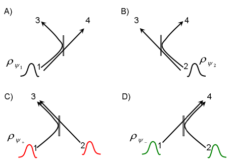
Figure 1:

in spatial regions where wave packets interfere or cross. The beam splitter example is actually reminiscent of the famous two slit interference experiment which was treated in details by Bohm and his followers. The trajectories look sometime ‘surrealistic’ but this is the price to pay to agree with both a wave and a particle in a $\lambda$-world.
Of course, if we throw away the $\xi\left(\alpha=\pm 1|\mathbf{a},\lambda\right)$ and use instead $P\left(\alpha=\pm 1|\mathbf{a},\lambda,\Psi_{0}\right)$ the whole reasoning of PBR collapses since we are not allowed to compare the states as we did in section 2.
Consider for example the orthogonal case. We now have instead of Eq. 4:

$$|\langle+|\Psi_{1}\rangle|^{2}=P(+|\Psi_{1})=\int P(+|\lambda,\Psi_{1})\rho_{1}(\lambda)d\lambda=0$$

$$|\langle-|\Psi_{2}\rangle|^{2}=P(-|\Psi_{2})=\int P(-|\lambda,\Psi_{2})\rho_{2}(\lambda)d\lambda=0.$$ (21)

We deduce of course that $P(+|\lambda,\Psi_{1})=0$ if $\rho_{1}(\lambda)\neq 0$ and $P(-|\lambda,\Psi_{2})=0$ if $\rho_{2}(\lambda)\neq 0$. Now If $\rho_{1}(\lambda)\cdot\rho_{2}(\lambda)\neq 0$ for some values of $\lambda$ (which means once again that $\rho_{1}$ and $\rho_{2}$ have intersecting support) then

$$P(+|\lambda,\Psi_{1})=P(-|\lambda,\Psi_{2})=0$$ (22)

for the $\lambda$s in the intersection of the two supports. What is fundamental here is that contrarily to what occurred for the models considered by PBR here Eq. 22 doesn’t imply any contradiction. Therefore the PBR theorem cannot be proven any more! All cases with either orthogonal or non orthogonal states can always be analyzed and criticized with the same method: If we substitute $\xi(\alpha|\lambda)$ by $P(\alpha|\lambda,\Psi)$ the PBR theorem can not be proven.
The theorem proposed by PBR is thus simply not general enough. It fits well with the XIX^th like hidden variable models but it is not in agreement with neo-classical model such as the one proposed by de Broglie and Bohm: QED reducio ad absurdum. In other words: the class of model PBR consider contradict wave particle duality (see our example with the beam splitter). I think that peoples who apply naively XIX^th century-like epistemic reasoning to quantum mechanics should seriously worry about PBR theorem (the others like Bohmian’s can sleep peacefully). Finally, we point out that since Bohm’s model is deterministic one must have

$$P\left(\alpha=\pm 1|\mathbf{a},\lambda,\Psi_{0}\right)=\delta_{\alpha,A(\lambda,\mathbf{a},\Psi_{0})}=0\textrm{ or }1$$ (23)

(where $\delta$ is the Kronecker symbol) since for one given $\lambda$ only one trajectory is allowed. Equivalently, the actual value $A(\lambda,\mathbf{a},\Psi_{0})=\sum_{\alpha}\alpha P\left(\alpha=\pm 1|\mathbf{a},\lambda,\Psi_{0}\right)$ can only takes one of the allowed eigenvalues $\alpha$ associated with the hermitian operator $A$. We show in the appendix that this is indeed the case for the particular half-spin model described by Bohm theory. However the result is actually very general.

IV Conclusion

Lets be positive: even if PBR theorem is generally wrong it is actually very interesting: it ruins the old fashion hidden variable approach in a nice way and show that there are some fundamental differences between classical $XIX^{th}$ century physics and the neo-classical mechanics proposed by Bohm and others. Both are based on realism. Both are admitting an ontic and epistemic parts. But now the wave function is part of the dynamic all the way along since it gives a contribution to the ontic state which subsequently affects the dynamic of the $\lambda$-particle. The initial Liouville approach separating the epistemic and the ontic part (i.e. $\rho$ and $q(t),p(t)$) appears to be wrong if we forget the wave function (i.e. a same $\lambda$ with different $\Psi_{0}$ will lead to different trajectories and density of probability). I think that PBR managed to do what was the original dream of von Neumann however both approaches are restricted to a very narrow class of hidden variable models (which are not orthogonal to each other by the way).

Appendix A Bohm’s deterministic model for a spin half particle (for those who are not already ‘Bohred’)

We consider the simple Q-Bit space for a single spin-$1/2$ Holland . In this model a neutral single particle with spin $1/2$ and mass $M$, is represented by a wave packet having two components

$$\Psi\left(\mathbf{x},t\right)=\left(\begin{array}[]{l}\psi_{\uparrow}\left(\mathbf{x},t\right)\\ \psi_{\downarrow}\left(\mathbf{x},t\right)\end{array}\right).$$ (26)

In presence of a magnetic field inside a Stern and Gerlach apparatus the two contributions of the wave packet are oriented in one or the other of the exits Scully ; Holland ; Holland2 , separating the trajectories associated with the two states $\uparrow$ and $\downarrow$. Naturally, any modifications of the magnetic field orientation change the analyzed basis $\uparrow,\downarrow$. Consequently in presence of the Stern and Gerlach apparatus analyzing the spin components along $\mathbf{a}$ and $-\mathbf{a}$ the density of probability $\rho\left(\mathbf{x},t\right)=|\psi_{\mathbf{a}}\left(\mathbf{x},t\right)|^{2}+|\psi_{-\mathbf{a}}\left(\mathbf{x},t\right)|^{2}$ depends explicitly on the orientation of the magnetic field and must be written $\rho\left(\mathbf{x},t,\mathbf{a}\right)$. The evolution of the wave function in the Stern and Gerlach apparatus is thus given by the pair of equations:

$$i\hbar\partial_{t}\psi_{\mathbf{a}}\left(\mathbf{x},t\right)=-\frac{\hbar^{2}\nabla^{2}}{2M}\psi_{\mathbf{a}}\left(\mathbf{x},t\right)+\mu(\mathbf{B}(\mathbf{x},t)\cdot\mathbf{a})\psi_{\mathbf{a}}\left(\mathbf{x},t\right)$$

$$i\hbar\partial_{t}\psi_{-\mathbf{a}}\left(\mathbf{x},t\right)=-\frac{\hbar^{2}\nabla^{2}}{2M}\psi_{-\mathbf{a}}\left(\mathbf{x},t\right)-\mu(\mathbf{B}(\mathbf{x},t)\cdot\mathbf{a})\psi_{-\mathbf{a}}\left(\mathbf{x},t\right)$$

($\mu$ is the magnetic dipole moment).
Now, Bohm says that the ontic state can be described dynamically as a point like object moving with the velocity $\mathbf{v}\left(\mathbf{x},t\right)=[\mathbf{J}/\rho]\left(\mathbf{x},t\right)$. Here

$$\mathbf{J}\left(\mathbf{x},t\right)=\hbar[|\psi_{+\mathbf{a}}\left(\mathbf{x},t\right)|^{2}\boldsymbol{\nabla}\phi_{+\mathbf{a}}\left(\mathbf{x},t\right)$$

$$+|\psi_{-\mathbf{a}}\left(\mathbf{x},t\right)|^{2}\boldsymbol{\nabla}\phi_{-\mathbf{a}}\left(\mathbf{x},t\right)]/M$$

and

$$\rho\left(\mathbf{x},t\right)=|\psi_{+\mathbf{a}}\left(\mathbf{x},t\right)|^{2}+|\psi_{-\mathbf{a}}\left(\mathbf{x},t\right)|^{2}$$ (29)

define the probability current and probability density respectively, and $\phi_{+\mathbf{a}},\phi_{-\mathbf{a}}$ are the phases of $\psi_{+\mathbf{a}},\psi_{-\mathbf{a}}$.
To understand some specificities of this theory I remind you that from Eqs A one deduce easily using the polar form of the wave function

$$-\partial_{t}|\psi_{\pm\mathbf{a}}\left(\mathbf{x},t\right)|^{2}=-\boldsymbol{\nabla}[|\psi_{\pm\mathbf{a}}\left(\mathbf{x},t\right)|^{2}\frac{\hbar}{M}\boldsymbol{\nabla}\phi_{\pm\mathbf{a}}\left(\mathbf{x},t\right)]$$

which is the local form of the conservation of probability rule. We also obtain a pair of de Broglie-Bohm version of Hamilton-Jacobi classical equations:

$$-\partial_{t}\hbar\phi_{\pm\mathbf{a}}\left(\mathbf{x},t\right)=\frac{(\boldsymbol{\nabla}\hbar\phi_{\pm\mathbf{a}}\left(\mathbf{x},t\right))^{2}}{2M}\pm\mu(\mathbf{B}(\mathbf{x},t)\cdot\mathbf{a})-\frac{\boldsymbol{\nabla}^{2}|\psi_{\pm\mathbf{a}}\left(\mathbf{x},t\right)|}{2M|\psi_{\pm\mathbf{a}}\left(\mathbf{x},t\right)|}$$ (31)

the quantum potential $\frac{\boldsymbol{\nabla}^{2}|\psi_{\pm\mathbf{a}}|}{2M|\psi_{\pm\mathbf{a}}|}$ is a specific feature of this theory which allows us to describe the quantum statistical properties of the half spin using a classical-like stochastic dynamic. Importantly this quantum potential depends on the absolute value of the wave function (up to an arbitrary constant) therefore the dynamical evolution will also depends on the wave function. This feature is completely different from what occurs in classical physics where the dynamic and the probability are respectively associated with a pure ontic an epistemic feature. In classical physics one is free to change the initial density of state without modifying the dynamic. However here the two features are unseparable since the wave function is part of the ontic and epistemic state at the same time. This feature has a strong consequence on the dynamical evolution which can also be seen more directly from the equation of motion

$$\frac{d}{dt}\mathbf{x}(t)=\frac{\hbar[|\psi_{+\mathbf{a}}\left(\mathbf{x},t\right)|^{2}\boldsymbol{\nabla}\phi_{+\mathbf{a}}\left(\mathbf{x},t\right)+|\psi_{-\mathbf{a}}\left(\mathbf{x},t\right)|^{2}\boldsymbol{\nabla}\phi_{-\mathbf{a}}\left(\mathbf{x},t\right)]}{M(|\psi_{+\mathbf{a}}\left(\mathbf{x},t\right)|^{2}+|\psi_{-\mathbf{a}}\left(\mathbf{x},t\right)|^{2})}=\frac{\hbar}{2M}\frac{\textrm{Im}[\Psi^{\dagger}\boldsymbol{\nabla}\Psi]}{\Psi^{\dagger}\Psi}\left(\mathbf{x},t\right).$$ (32)

In order to integrate even formally this equation we first have to integrate the Schrodinger equation and we will obtain solution of the form $\psi_{\pm\mathbf{a}}\left(\mathbf{x},t\right)=\int d^{3}\mathbf{x}^{\prime}K_{\pm\mathbf{a}}\left(\mathbf{x},t,\mathbf{x}^{\prime},t_{0}\right)\psi_{\pm\mathbf{a}}\left(\mathbf{x}^{\prime},t_{0}\right)$ where the kernel $K_{\pm\mathbf{a}}\left(\mathbf{x},t,\mathbf{x}^{\prime},t_{0}\right)$ can be evaluated from the Green function. Inserting these solutions in Eq. 32 leads to a new differential equation for $\mathbf{x}(t)$ which reads formally as:

$$\frac{d}{dt}\mathbf{x}(t)=\mathbf{G}_{\mathbf{a}}(\mathbf{x}(t),t,\{\Psi^{\dagger}(\mathbf{x}^{\prime},t_{0}),\Psi(\mathbf{x}^{\prime},t_{0})\}_{\mathbf{x}^{\prime}}\forall\mathbf{x}^{\prime}).$$ (33)

This is a first order equation which not only depends on $\mathbf{x}(t)$ at the same given time $t$ (i.e. when the derivative is evaluated) but also require the knowledge of the wave function and its complex conjugate evaluated for every position $\mathbf{x}^{\prime}$ of the evolution space at the initial time $t_{0}$. This set of initial values $\{\Psi^{\dagger}(\mathbf{x}^{\prime},t_{0}),\Psi(\mathbf{x}^{\prime},t_{0})\}_{\mathbf{x}^{\prime}}$ plays therefore the role of additional constants of motion. Therefore the complete trajectory wil be given by a functional having the general form

$$\mathbf{x}(t)=\mathbf{F}_{\mathbf{a}}(t;\mathbf{x}_{0}(t),t_{0},\{\Psi^{\dagger}(\mathbf{x}^{\prime},t_{0}),\Psi(\mathbf{x}^{\prime},t_{0})\}_{\mathbf{x}^{\prime}}\forall\mathbf{x}^{\prime}).$$ (34)

Now, in Bohm’s model we can define an instantaneous spin vector

$$\mathbf{S}\left(\mathbf{x},t,\mathbf{a}\right)=\frac{\Psi^{\dagger}\boldsymbol{\sigma}\Psi}{\rho\left(\mathbf{x},t,\mathbf{a}\right)}.$$ (35)

The projection $\Sigma\left(\mathbf{x},t,\mathbf{a}\right)=\mathbf{S}\left(\mathbf{x},t,\mathbf{a}\right)\cdot\mathbf{a}$ spans a continuum of values during the interaction with the magnetic field but at end of the measure (i. e. at $t=\infty$) we have $\Sigma=\pm 1$ corresponding to the spin observable $A=\pm 1$. We can naturally define the mean value of the spin projection $\Sigma$ by

$$E_{\Psi}\left(\sigma\right)=\langle\Psi|\boldsymbol{\sigma}\cdot\mathbf{a}|\Psi\rangle=\int\Sigma\left(\mathbf{x},t,\mathbf{a}\right)\rho\left(\mathbf{x},t,\mathbf{a}\right)d^{3}\mathbf{x}.$$

We can always define univocally the actual position $\mathbf{x}\left(t\right)$ measured for example at $t=+\infty$ by a function of the initial coordinate $\mathbf{x}_{0}=\lambda$ of the particle at a time $t_{0}\rightarrow-\infty$, i. e. a long time before that the particle enters in the Stern and Gerlach apparatus. Due to the conservation of probability requirement the number of states defined by $\rho\left(\mathbf{x}_{0},t_{0}\right)\delta^{3}\mathbf{x}_{0}$ in the elementary volume $\delta^{3}\mathbf{x}_{0}$ is naturally identical to $\rho\left(\mathbf{x}\left(t\right),t,\mathbf{a}\right)\delta^{3}\mathbf{x}\left(t\right)$ i. e. :

$$\rho\left(\mathbf{x}\left(t\right),t,\mathbf{a}\right)\delta^{3}\mathbf{x}\left(t\right)=\rho\left(\mathbf{x}_{0}(t_{0}),t_{0}\right)\delta^{3}\mathbf{x}_{0}\left(t_{0}\right).$$ (37)

This result is of course well known in fluid dynamics where it is associated to the names of Euler and Lagrange (the so called Euler-Lagrange coordinates). This law can also be written

$$\int_{\delta V}\rho\left(\mathbf{x}^{\prime},t,\mathbf{a}\right)d^{3}\mathbf{x}^{\prime}=\int[\int_{\delta V}\delta^{3}(\mathbf{x}^{\prime}-\mathbf{x}(t))d^{3}\mathbf{x}^{\prime}]\rho\left(\mathbf{x}(t),t,\mathbf{a}\right)d^{3}\mathbf{x}(t)$$

$$=\int[\int_{\delta V}\delta^{3}(\mathbf{x}^{\prime}-\mathbf{F}_{\mathbf{a}}(t;\mathbf{x}_{0}(t),t_{0},\{\Psi^{\dagger}(\mathbf{x}^{\prime},t_{0}),\Psi(\mathbf{x}^{\prime},t_{0})\}_{\mathbf{x}^{\prime}}\forall\mathbf{x}^{\prime}))d^{3}\mathbf{x}^{\prime}]\rho\left(\mathbf{x}_{0}(t_{0}),t_{0}\right)d^{3}\mathbf{x}_{0}(t_{0})$$ (38)

The second line in this equation is deduced from Eq. 34. This expression is therefore a generalization for the continuous observable $\mathbf{x}$ of Eq. 18 which is valid only for dichotomic observable. Similarly $\Sigma\left(\mathbf{x}\left(t\right),t,\mathbf{a}\right)$ can be expressed as a function of the initial coordinates of the particle and can be written $A\left(\mathbf{x}_{0}(t_{0}),t_{0},\{\Psi^{\dagger}(\mathbf{x}^{\prime},t_{0}),\Psi(\mathbf{x}^{\prime},t_{0})\}_{\mathbf{x}^{\prime}}\forall\mathbf{x}^{\prime},t,\mathbf{a},\right)$. If we consider now the expectation value $\langle\Psi|\boldsymbol{\sigma}\cdot\mathbf{a}|\Psi\rangle$, we can write

$$E_{\Psi}\left(\sigma\right)=\langle\Psi|\boldsymbol{\sigma}\cdot\mathbf{a}|\Psi\rangle=\int\Sigma\left(\mathbf{x},t,\mathbf{a}\right)\rho\left(\mathbf{x},t,\mathbf{a}\right)d^{3}\mathbf{x}$$

$$=\int A\left(\mathbf{x}_{0}(t_{0}),t_{0},\{\Psi^{\dagger}(\mathbf{x}^{\prime},t_{0}),\Psi(\mathbf{x}^{\prime},t_{0})\}_{\mathbf{x}^{\prime}}\forall\mathbf{x}^{\prime},t,\mathbf{a}\right)\rho\left(\mathbf{x}_{0},t_{0}\right)d^{3}\mathbf{x}_{0}(t_{0}).$$ (39)

If we choose $t=+\infty$ then $A=\pm 1$ and we have the complete definition of Bell (with now $\rho(\lambda)$ independent of $\mathbf{a}$ as desired).
One can also define

$$\mathcal{P}(\alpha=\pm 1,\mathbf{a})=\frac{1\pm\langle\Psi|\boldsymbol{\sigma}\cdot\mathbf{a}|\Psi\rangle}{2}=\int\frac{(1\mp\Sigma\left(\mathbf{x},t,\mathbf{a}\right))}{2}\rho\left(\mathbf{x},t,\mathbf{a}\right)d^{3}\mathbf{x}$$

$$=\int\frac{(1\pm A\left(\mathbf{x}_{0}(t_{0}),t_{0},\{\Psi^{\dagger}(\mathbf{x}^{\prime},t_{0}),\Psi(\mathbf{x}^{\prime},t_{0})\}_{\mathbf{x}^{\prime}}\forall\mathbf{x}^{\prime},t,\mathbf{a}\right))}{2}\rho\left(\mathbf{x}_{0},t_{0}\right)d^{3}\mathbf{x}_{0}(t_{0}).$$ (40)

This quantity approaches asymptotically the definition of the projector operator on the $\pm\mathbf{a}$ direction and therefore gives us the probability for the dichotomic spin projection observable. The quantity

$$\frac{(1\pm A)}{2}=\delta_{\alpha=\pm 1,A}=0\textrm{ or }1$$ (41)

is indeed the conditional probability $P_{1}\left(\alpha=\pm 1|\mathbf{a},\lambda,\Psi\right)$ discussed in the manuscript (see Eq. 18).

References

• (1) M. F. Pusey, J. Barrett and T. Rudolph, “The quantum state cannot be interpreted statistically”, arXiv:1111.3328.
• (2) N. Harrigan andR. W. Spekkens, Found. Phys. 40, 125 (2010),
• (3) P. R. Holland, The Quantum Theory of Motion, Cambridge University Press, Cambridge, 1993.
• (4) D. Bohm, B. J. Hiley and P. N. Kaloyerou, Phys. Rep. 144 (1987) 321.
• (5) M. O. Scully, W. E. Lamb, and A. O. Barut, Found. Phys. 17, 575 (1987).
• (6) C. Dewdney, P. R. Holland and A. Kyprianidis Phys. Lett. A119, 259 (1986).