Recent results of Milagro, Tibet, ARGO-YBJ and IceCube experiments on the small-scale anisotropy of Galactic cosmic rays (CRs) with energies from units up to a few hundred TeV arise a question on a possible nature of the observed phenomenon, as well as on the anisotropy of CRs at higher energies. An analysis of a small-scale anisotropy of CRs with energies at around PeV registered with the EAS MSU array presented in the article, reveals a number of regions with an excessive flux. A typical size of the regions varies from $3^{\circ}$ up to $12^{\circ}$. We study correlation of these regions with positions of potential astrophysical sources of CRs and discuss a possible origin of the observed anisotropy.

Introduction

In the last few years, a big interest was attracted to results of Milagro (Atkins et al., 2004; Saz Parkinson, 2005; Abdo et al., 2007, 2008), Tibet AS$\gamma$ (Amenomori et al., 2005, 2006, 2009), Super-Kamiokande (Oyama, 2006; Guillian et al., 2007) and ARGO-YBJ (Di Sciascio, Iuppa, 2011) experiments on the anisotropy of cosmic rays (CRs) with energies from units up to a few tens TeV at scales up to $30^{\circ}$. As is witnessed by the results published, a number of regions with either an excess or deficit of the CR flux of the above energies is observed in the Northern hemisphere, and the shape, location and the degree of magnitude depend on the energy of CRs. Recent observations held with IceCube demonstrate that the small-scale anisotropy takes place in the Southern hemisphere either, and that the observed sky map for cosmic rays with the median energy 20 TeV differs significantly from that at 400 TeV (Abbasi et al., 2011a,b).

The above results have attracted considerable attention because, on the one hand, they shed additional light on the structure of the interstellar magnetic field, and on the other hand, they provide information to solve the problem of the origin of cosmic rays, which remains open for many years. Recall that the most widely spread model is the model of diffusive acceleration of charged particles on shock fronts generated by explosions of supernovae, see, e.g., the review by Hillas (2005). It is thought that CRs can be accelerated in supernova remnants (SNRs) up to energies of the order of 1 PeV and even higher energies under certain circumstances (Ptuskin et al., 2011). Still, experimental data that prove that TeV–PeV CRs are accelerated in SNRs are rather poor and are mostly confined to observations of SNRs W44 and G120.1+1.4 (SN 1572, Tycho SNR) in gamma rays (Giuliani et al., 2011; Morlino, Caprioli, 2011). Even in these cases, one can only speak about acceleration of hadrons up to energies of about 0.5 PeV. The situation with the majority of known Galactic SNRs remains unclear. In any case, a proof of the fact that CRs are accelerated in supernova remnants up to energies of the order of PeV will not imply that these are supernovae that are the main or the only source of Galactic CRs of these energies. By this reason, other possible astrophysical sources of CRs but not only isolated SNRs are considered.

Models most close to SNRs in the sense of particle acceleration are those that employ OB-associations, i.e., clusters of the most massive and hot stars of spectral classes O and B (see the works by Bykov et al., (1995), Parizot et al., (2004), Binns et al., (2008)), and superbubbles formed by them (see, e.g., Higdon and Lingenfelter, 2005). There are some facts that witness in favour of CR acceleration in superbubbles. For example, recent observations performed with the orbital gamma-ray telescope Fermi-LAT have demonstrated that a region located approximately between OB-association Cyg OB2 and SNR $\gamma$-Cygni is a place of effective CR acceleration (Ackermann et al., 2011). On the other hand, data on the composition of CRs show that most likely, superbubbles are not the main source of Galactic cosmic rays (Prantzos, 2011).

Another possible source of CRs are pulsars. Shortly after pulsars were discovered and identified with neutron stars, it was demonstrated they can be effective accelerators of CRs (Gunn, Ostriker, 1969). This has attracted interest immediately, and there appeared a number of works that analysed a possible correlation between arrival directions of CRs and coordinates of pulsars known at that time (Andrews et al., 1970; Suga et al., 1971). Interest to pulsars as possible sources of CRs with energies $\gtrsim 10^{14}$ eV did not vanish subsequently, see, e.g, works by Blasi et al. (2000), Giller and Lipski (2002), Bhadra (2003, 2006), Erlykin and Wolfendale (2004). Models considered included acceleration both in pulsars surrounded by wind nebulae (e.g., the Crab nebula) and by isolated pulsars. In particular, Bhadra (2003) considered the Geminga pulsar as a possible candidate for being the single source of the knee at 3 PeV. Other authors argue that the presence of a pulsar is essential for an effective acceleration of CRs in a supernova remnant (e.g., Neronov, Semikoz, 2012).

The aforementioned results on the small-scale anisotropy of TeV CRs appeared to be rather unexpected because trajectories of charged particles of cosmic rays of these energies are entangled in interstellar magnetic fields so that their arrival directions to Earth are expected to be isotropic. Still, a comparison of arrival directions of CRs with location of their possible astrophysical sources can help to reveal their origin in case of certain configurations of magnetic fields as well as in case when a considerable part of CRs consists of neutral particles. There is also a point of view that the Galactic magnetic field can be uniform at scales of the order $\gtrsim 300$ pc, so that charged particles can keep directions of their movement within this scale (Oyama, 2006). All this motivated us to perform a new analysis of the complete data set of the EAS MSU array. In our previous works dedicated to examination of arrival directions of CRs with energies in the PeV range registered with the EAS MSU array (Zotov, Kulikov, 2009, 2010, 2011) and the EAS–1000 Prototype array (Kulikov, Zotov, 2004; Zotov, Kulikov, 2004, 2007) we presented a whole number of small-scale regions of excessive flux (REFs) of CRs. In the present work, we confirm the existence of such regions in the experimental data of the EAS MSU array with the statistical significance from $3\sigma$ up to $4.95\sigma$ and analyse their correlation with location of Galactic SNRs, pulsars, OB-associations and open clusters. It happens that the majority of regions found can be matched to astrophysical objects of at least one of the above types. Possible nature of the observed anisotropy is discussed in conclusion.

1 Experimental Data and Method of The Investigation

The analysed data set consists of 513,602 showers registered with the EAS MSU array in 1984–1990. A description of the array can be found in the paper by Vernov et al. (1979). All EAS selected for the analysis satisfy a number of quality criteria and have zenith angles $\theta\leq 45^{\circ}$. The median number of the full number of charged particles at the level of observation equals approximately $1.6\times 10^{5}$. According to the modern models of hadron interactions and data on mass composition of primary cosmic rays, this value corresponds to the energy of primary protons $E_{0}\approx 1.7\times 10^{15}$ eV with an accuracy of the order of 10%–20%. An error in determination of arrival directions is estimated to be of the order of $3^{\circ}$.

The investigation is based on the method by Alexandreas et al. (1991), which was developed for the analysis of arrival directions of EAS registered with the CYGNUS array, and since then has been used multiple times for the analysis of data of other experiments. The idea of the method is as follows. To every shower in the experimental data set, an arrival time of another shower is assigned in a pseudo-random way. After this, new equatorial coordinates $(\alpha,~{}\delta)$ are calculated for the whole data set basing on the original zenith and azimuthal angles $(\theta,\phi)$ and assigned arrival times. This results in a “mixed” map of arrival directions that differs from the original one but has the same distribution in declination $\delta$. The mixing of the real map is performed multiple times, and the mixed maps are averaged in order to reduce the dependence of the result on the choice of arrival times. The method is based on an assumption that the resulting mean “background” map has most of the properties of an isotropic background, and presents the distribution of arrival directions of cosmic rays that would be registered with the array in case there is no anisotropy. A measure of difference between any two regions of the two maps located within the same boundaries is defined as $S=(N_{\mathrm{real}}-N_{\mathrm{bg}})/\sqrt{N_{\mathrm{bg}}}$, where $N_{\mathrm{real}}$ and $N_{\mathrm{bg}}$ are the number of EAS inside the same region in the real and background maps respectively. As a rule, selection of regions of excessive flux is performed basing on the condition $S>3$.

To search for REFs, we divided both maps into “basic” cells with the size $0.5^{\circ}\times 0.5^{\circ}$, which were used then to form larger rectangular regions with the size $\Delta\delta=3^{\circ}\dots 15^{\circ}$. The width of these regions was chosen so that for a given $\Delta\delta$ and $\delta=0^{\circ}$ the area of the region differed from the area of a square with the same height by at most 1/6, and was kept approximately constant for growing $\delta$. A detailed description of the method can be found in the paper by Zotov, Kulikov (2010).

The method of Alexandreas et al. does not provide a direct answer to the question about the chance probability of appearance of an REF. It can be calculated basing on the value of $S$, which is an estimate of the standard deviation of a sample and thus acts as a statistical significance. By this, it is implicitly assumed that the deviation of $N_{\mathrm{real}}$ from $N_{\mathrm{bg}}$ has a Gaussian distribution. Hence, it is assumed the chance probability of an REF to appear is less than $1-0.9973$ providing it was selected at $S>3$.

One can also estimate the chance probability of an appearance of an REF from the number of EAS inside, as is suggested by the following simple method based on the binomial distribution (Zotov, Kulikov, 2009). Let a shower axis getting inside a region be a success. The number of trials equals the number of showers $N$ in the given data set, and an estimate of success for a fixed region equals $\tilde{p}=N_{\mathrm{bg}}/N$, where $N_{\mathrm{bg}}$ is the number of showers in the region of the background map. The assumption is based on the fact that in the method of Alexandreas et al., $N_{\mathrm{bg}}$ is considered to be an expected number of showers in a cell. Obviously, the chance probability of finding exactly $N_{\mathrm{real}}$ EAS in a region equals

$$P(\nu=N_{\mathrm{real}})=C(N,N_{\mathrm{real}})\tilde{p}^{N_{\mathrm{real}}}(1-\tilde{p})^{N-N_{\mathrm{real}}},$$

where $\nu$ is a random variable equal to the number of successes in the binomial model, and $C(N,N_{\mathrm{real}})$ is the corresponding binomial coefficient. It is more interesting to consider a probability that there are at most $N_{\mathrm{real}}$ showers in the region $P_{\mathrm{r}}=P(\nu\leq N_{\mathrm{real}})$. The analysis performed and the data presented below demonstrate that values of $P_{\mathrm{r}}$ correlate well with the values of chance probabilities calculated on the basis of the significance $S$.

The regions of excessive flux of CRs found in the data set of the EAS MSU array do not solely consist of basic cells with an excess of registered EAS over the background flux with a significance $S>3$. In a typical REF, there are basic cells with an excess as well as a deficit of EAS with respect to the background level. Employment of the pure criterion $S>3$ can result in a region selected as an REF solely due to a huge irregularity of the distribution of arrival directions in declination $\delta$. In order to improve the robustness of selection of REFs, we tried a number of additional quantities. The most productive of them is the probability $P_{\mathrm{bc}}=P(\xi<N_{\mathrm{bc}}^{+})$, calculated from the following binomial model. Let $\xi$ be a random variable equal to the number of basic cells of the given region with an excess of EAS over the background values, and $N_{\mathrm{bc}}^{+}$ is the corresponding experimental value. The number of trials equals the number of basic cells in the REF. It is natural to assume the probability of success to be equal to 1/2. In the results presented below, all REFs satisfy a condition $P_{\mathrm{bc}}>0.9545$, which corresponds to the significance $>2\sigma$ for the Gaussian distribution. We thus reduced the chance that an REF is selected solely due to the non-uniformity of the EAS distribution with respect to $\delta$.

2 The Main Results

In what follows, we consider REFs found in the experimental data of the EAS MSU array under the following conditions:

$$N_{\mathrm{real}}>100,\quad S>3,\quad P_{\mathrm{bc}}>0.9545.$$

These conditions are satisfied for 1073 cells with $\Delta\delta=3^{\circ}\dots 11.5^{\circ}$ that form 41 non-overlapping regions, see Fig. 1. All the REFs are located in the strip with declination $\delta=14.5^{\circ}\dots 81^{\circ}$ and have an area in the range from 7.5 to 128 square degrees. The number of EAS inside selected cells varies from 101 up to 5552, while background values vary from 67 to 5326. Some parameters of the REFs are presented in Table 1. We remark that regions that consist of a single cell satisfying the above conditions (REFs 3, 7, 27, 31, 34 and 36) are not “outbursts” but parts of larger regions with $S$ slightly less than 3.

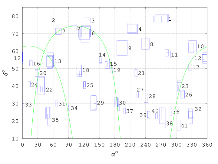
Figure 1: The regions of excessive flux of cosmic rays according to the data of the EAS MSU array, in equatorial coordinates. The curves at the left and right sides of the Figure show the Galactic plane, the $\cap$-like curve shows the Supergalactic plane.

It is interesting that regions 5, 6, 9, 13, 20, 21, 25, as well as adjacent regions 23 and 26 are mainly made up of showers with the particle number above the median value, while regions 8, 10, 12, 19, 22, 29, 32 and 38 with those below the median.

As is clear from Table 1, regions 40 and 41 are excluded from the selection if one replaces the condition $N_{\mathrm{real}}>100$ with $N_{\mathrm{bg}}>100$.

Table 1: Some parameters of the REFs of CRs according to the data of the EAS MSU array. Notation: $\alpha$ and $\delta$ are the ranges of the corresponding equatorial coordinates; $N_{\mathrm{real}}$, $N_{\mathrm{bg}}$ are the ranges of the experimental and background flux of EAS in rectangular regions with excessive flux of CRs that constitute the REF respectively; $\max S$, $\max P_{\mathrm{r}}$, $\max P_{\mathrm{bc}}$ are the maximum values of the respective variables for the rectangular regions with $\Delta\delta\geq 3^{\circ}$ that constitute the REFs.

REF	$\alpha,\,^{\circ}$	$\delta,\,^{\circ}$	$N_{\mathrm{real}}$	$N_{\mathrm{bg}}$	$\max S$	$\max P_{\mathrm{r}}$	$\max P_{\mathrm{bc}}$
1	256.0…284.5	76.5…81.0	442…1042	375.2…942.8	3.93	0.999939	0.988350
2	42.0…56.0	76.0…79.5	454…598	393.3…528.9	3.16	0.999081	0.995984
3	120.0…133.0	76.0…79.0	503	438.8	3.07	0.998763	0.990027
4	204.0…224.5	70.0…76.0	550…1852	480.2…1726.0	3.51	0.999741	0.996050
5	93.0…105.0	71.5…75.5	576…861	507.0…776.1	3.10	0.998903	0.996077
6	109.5…133.0	65.0…74.5	537…2727	470.0…2573.8	4.23	0.999985	0.999596
7	64.5…76.0	69.5…73.0	853	768.3	3.06	0.998774	0.986488
8	232.0…247.5	61.0…67.0	654…2722	579.7…2565.9	3.47	0.999717	0.984226
9	184.0…204.5	57.5…66.0	4093…5552	3904.6…5326.2	3.09	0.999026	0.981344
10	324.0…339.0	59.0…66.0	1418…2957	1309.0…2788.4	3.29	0.999453	0.993782
11	278.0…288.5	55.5…61.0	518…1146	449.6…1025.1	4.48	0.999994	0.996891
12	350.0…361.0	53.0…59.5	624…1820	549.6…1692.3	3.46	0.999684	0.989870
13	47.0…61.0	50.0…59.0	1607…3421	1481.8…3242.5	3.59	0.999817	0.991294
14	150.0…155.5	53.0…56.5	511…610	441.3…539.5	3.32	0.999454	0.982209
15	161.0…169.5	50.0…55.5	548…1464	476.8…1352.8	3.26	0.999344	0.995273
16	14.0…19.5	51.5…54.5	574…627	504.7…555.1	3.09	0.998853	0.974053
17	324.0…330.0	49.0…52.5	735…797	655.1…714.6	3.12	0.998992	0.968514
18	106.0…115.5	45.5…52.0	478…2200	415.8…2063.0	3.13	0.999061	0.993752
19	171.0…176.0	47.5…51.0	647…717	574.8…638.8	3.09	0.998898	0.988769
20	24.5…32.0	45.5…49.5	479…991	409.5…897.6	3.88	0.999926	0.993358
21	219.0…224.0	45.5…49.5	478…767	416.2…687.0	3.31	0.999439	0.997242
22	30.0…44.5	35.0…45.5	332…3905	279.0…3703.6	3.76	0.999884	0.985960
23	301.5…309.0	37.0…43.0	425…1253	366.5…1148.0	3.28	0.999389	0.985377
24	11.0…15.5	39.5…42.5	373…484	314.4…404.1	3.97	0.999949	0.979888
25	119.0…123.5	38.5…42.5	424…618	366.2…539.6	3.38	0.999564	0.999641
26	308.0…316.0	33.0…37.5	294…605	245.7…533.9	3.63	0.999812	0.987770
27	223.0…226.5	33.5…36.5	278	231.6	3.05	0.998636	0.978221
28	237.0…245.0	30.5…36.0	256…875	210.7…789.1	3.35	0.999492	0.999657
29	133.0…144.0	26.0…34.5	159…1613	121.6…1494.8	3.39	0.999508	0.994773
30	180.0…189.5	26.0…33.5	162…570	126.5…501.8	3.55	0.999747	0.996845
31	65.0…69.0	28.0…32.0	292	241.4	3.26	0.999298	0.970029
32	323.5…334.5	18.5…32.0	101…1148	67.3…1049.3	4.95	0.999998	0.999844
33	0.0…3.5	27.5…31.5	190…221	150.6…180.0	3.21	0.999141	0.990240
34	90.0…93.0	26.0…29.0	144	105.3	3.77	0.999858	0.967377
35	45.0…56.0	17.5…28.0	103…481	75.4…418.0	3.55	0.999716	0.999530
36	286.0…291.0	23.0…28.0	264	218.1	3.11	0.998857	0.971556
37	197.5…201.0	24.0…27.5	137…155	103.6…117.8	3.42	0.999551	0.957283
38	266.5…278.5	16.0…27.5	144…874	111.6…789.3	3.20	0.999180	0.994773
39	243.0…248.5	21.5…25.5	101…160	72.9…126.0	3.37	0.999451	0.990240
40	259.5…263.5	21.0…24.5	106…118	77.1…88.1	3.30	0.999283	0.959287
41	301.5…307.5	14.5…20.5	107…131	78.6…98.7	3.25	0.999199	0.977557

2.1 Supernova Remnants

As it was already discussed above, supernova remnants are the main candidates for being the sources of Galactic CRs with energies $\lesssim 1$ PeV. In Fig. 2, coordinates of Galactic SNRs located in the field of observation are shown according to the catalogue by Green (2009). Numbers denote REFs that have at least one SNR at the angular distance $\leq 3^{\circ}$.

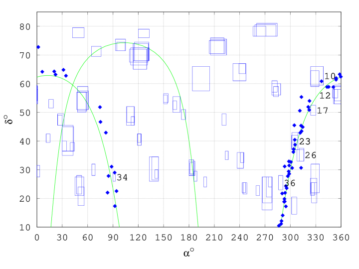
Figure 2: Coordinates of Galactic SNRs located in the field of observation, according to the catalogue by Green (2009). The numbers are shown for REFs that have at least one SNR in their 3-degree neighbourhood.

There are seven such regions. All of them are located near the Galactic plane. Twenty-one of 58 SNRs in the field of observation belong to the 3-degree neighbourhoods of the regions of excessive flux. Five SNRs lie inside REFs. One of the SNRs (G76.9+1.0) is located in the vicinity of two REFs. It lies inside REF 23 and, simultaneously, at the angular distance $\rho\approx 2.6^{\circ}$ from the adjacent REF 26.

Some parameters of the selected SNRs are presented in Table 2.

Table 2: Some parameters of SNRs in the 3-degree neighbourhood of the REFs. Notation: $\alpha,^{\circ}$, $\delta,^{\circ}$ are the equatorial coordinates of an object; $\rho,^{\circ}$ is the angular distance from an SNR to the given REF (0 means the object is within the boundaries of the REF); $d$ is the distance from the REF to the Solar system, kpc; Size,^′ is the angular size of the remnant, in arcminutes; Type of the SNR: “S” or “F” if the remnant shows a “shell” or “filled-centre” structure, or “C” if it shows “composite” radio structure with a combination of shell and filled-centre characteristics; the question sign (?) after S, F, C denotes some uncertainty in the type of an SNR; a single ? denotes objects that are regarded to be supernova remnants though their nature is not well-understood (Green, 2009).

REF	Name	$\alpha,^{\circ}$	$\delta,^{\circ}$	$\rho,^{\circ}$	$d$, kpc	Size,′	Type
10	G106.3+2.7	336.87	60.83	0		60x24	C?
	G108.2-0.6	343.42	58.83	2.36	3.2	70x54	S
12	G109.1-1.0 (CTB 109)	345.40	58.88	2.56	3	28	S
	G111.7-2.1 (Cas A, 3C461)	350.86	58.80	0.59	3.4	5	S
	G113.0+0.2	354.15	61.37	1.87	3.1	40x17?	?
	G114.3+0.3	354.25	61.92	2.42	0.7	90x55	S
	G116.9+0.2 (CTB 1)	359.79	62.43	2.93	1.6	34	S
17	G93.7-0.2 (CTB 104A)	322.33	50.83	1.05	1.5	80	S
	G94.0+1.0	321.21	51.88	1.72	5.2	30x25	S
	G96.0+2.0	322.62	53.98	1.69	4	26	S
23	G73.9+0.9	303.56	36.20	0.80		27	S?
	G74.9+1.2 (CTB 87)	304.01	37.20	0	6.1–12	8x6	F
	G76.9+1.0	305.58	38.72	0		9	?
	G78.2+2.1 ($\gamma$-Cygni)	305.21	40.43	0		60	S
	G82.2+5.3 (CTB 88)	304.75	45.50	2.50		95x65	S
	G83.0-0.3	311.73	42.87	2.00		9x7	S
26	G74.0-8.5 (Cygnus Loop)	312.75	30.67	2.33	0.44	230x160	S
	G76.9+1.0	305.58	38.72	2.57		9	?
34	G179.0+2.6	88.42	31.08	2.49		70	S?
	G182.4+4.3	92.04	29.00	0		50	S
36	G55.7+3.4	290.33	21.73	1.27		23	S
	G57.2+0.8	293.75	21.95	2.75		12?	S?

The biggest number of SNRs is “collected” by REF 23, which is located in the Galactic plane in the direction to a region in constellation Cygnus with well-known X-ray binaries Cygnus X-1 and Cygnus X-3, about 800 regions of ionized hydrogen HII, a big number of Wolf–Rayet stars and a number of OB-associations. Three supernova remnants lie inside this REF, three other are located at angular distances from 0.8^∘ to 2.5^∘. The most well-studied of them is $\gamma$-Cygni (G78.2+2.1), inside which sources of X-ray and gamma-ray emission were registered. A considerable attention is also attracted by SNR G76.9+1.0, which contains a high-energy pulsar discovered recently (Arzoumanian et al., 2011), see below. It is interesting that Cygnus X-3 lies within the boundaries of REF 23, and a well-known X-ray source Cygnus X-1, which is likely to consist of a massive black hole and a giant companion star, is only at $2.4^{\circ}$ to the south, and is situated comparatively close to the Solar system. The latest estimates give a distance of the order of 1.86 kpc (Reid et al., 2011).

REF 23 adjoins REF 26, which has another SNR located at $\rho\approx 2.3^{\circ}$ to the south, namely, Cygnus Loop (G74.0-8.5), that is a subject of numerous investigations. Cygnus Loop contains a number of X-ray and radio sources, and its distance to the Solar system is estimated to be as small as 0.44 kpc.

The second in the number of neighbouring SNRs is region 12. The closest remnant, located at only $\rho=0.6^{\circ}$, is Cassiopeia A, one of the most widely discussed candidates for being a source of Galactic cosmic rays. SNR G114.3+0.3, situated at 0.7 kpc from the Solar system, is also worth mentioning. It is interesting that all SNRs in the neighbourhood of this region but Cassiopeia A have pulsars within or close to their boundaries. This is not true for the majority of SNRs located in the neighbourhood of the other REFs. Besides the SNRs in the vicinity of REF 12 and the aforementioned SNR G76.9+1.0, only SNRs G106.3+2.7 (REF 10) and G55.7+3.4 (REF 36) are associated with pulsars.

An extension of the analysed neighbourhood of the REFs up to $4^{\circ}$ leads to selecting seven more SNRs. Among them, there is a well-known remnant IC443 (G189.1+3.0), which contains an X-ray binary as a compact central object. SNR IC443 is located at the angular distance $\rho\approx 3.6^{\circ}$ to the south from REF 34, and its distance from the Solar system is estimated to be from 0.7 kpc to 2 kpc. SNR S147, which is comparatively close to the Solar system, lies at the angular distance $\rho\approx 4.6^{\circ}$ to the west from REF 34. The estimates of the distance to S147 vary from 0.36 kpc to 0.88 kpc. It is interesting to mention that SNRs G106.3+2.7 (REF 10), G109.1-1.0, G111.7-2.1 (Cas A) (REF 12), G94.0+1.0 (REF 17), G74.9+1.2, G78.2+2.1 ($\gamma$-Cygni) (REF 23), G74.0-8.5 (Cygnus Loop) (REF 26) and IC443 have molecular clouds in their vicinity (Jiang et al., 2010).

2.2 Pulsars

There were 355 Galactic pulsars known in the field $\delta>10^{\circ}$ at the time of the investigation (Manchester et al., 2005), and 115 of them were found to belong to the 3-degree neighbourhoods of 28 of the REFs. Fifty of them lie within the boundaries of 15 REFs, eight pulsars are common for several regions, see Fig. 3. The number of selected pulsars grows up to 155 if one extends the size of the studied neighbourhoods to $4^{\circ}$. Remark that regions 6, 11 and 32 contain sub-regions selected with a statistical significance $>4\sigma$, see our previous work (Zotov, Kulikov, 2011).

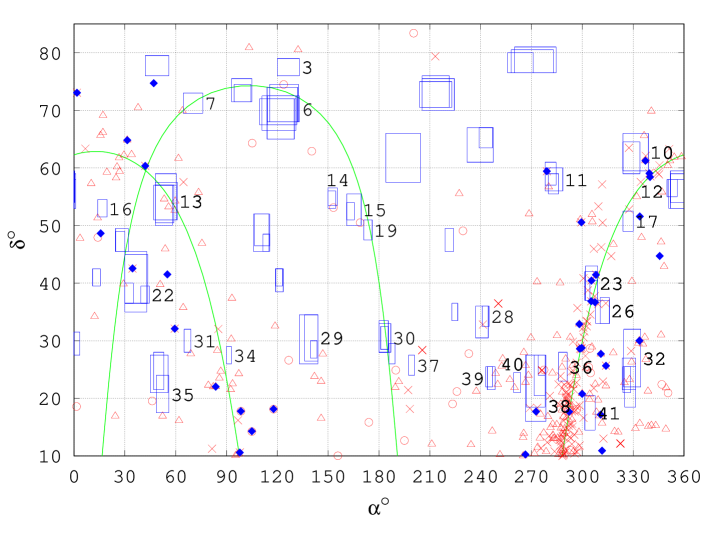
Figure 3: The REFs and Galactic pulsars (Manchester et al., 2005). The numbers are shown for the REFs that have pulsars in their 3-degree neighbourhood. Different symbols are used for pulsars located at different distances $d$ from the Solar system: $\circ$ for $d\leq 1$ kpc, $\triangle$ for $1<d\leq 5$ kpc, $\times$ for pulsars at $d>5$ or at unknown distance. Dark diamonds denote coordinates of gamma-ray pulsars according to the Fermi LAT second source catalog (Abdo et al., 2011).

Though pulsars are considered as possible sources of CRs since late 1960s, there is still no generally accepted model of acceleration of charged particles in the vicinity of isolated pulsars. To estimate the maximum energy of a particle accelerated near the light cylinder of a pulsar, we employed an expression by Blasi et al. (2000) that can be written as follows: $E_{\max}=0.34\,Z\,B\,\Omega^{2}$ eV, where $Z$ is the charge number of the particle; $B$ is the strength of the surface magnetic field: $B=3.2\times 10^{19}\sqrt{P\dot{P}}$, G; $P$ is the barycentric period of rotation of the pulsar, s; $\Omega$ is the angular velocity of the pulsar, rad s^-1, and the radius of the pulsar equals $10^{6}$ cm. The expression was obtained under the assumption that most of the magnetic field energy in the pulsar wind zone is transformed into the kinetic energy of the particles, and the density of electron-positron pairs does not exceed $10^{-5}$ of that of ions of iron.

The maximum energy of protons accelerated in the selected 115 pulsars varies from $2.2\times 10^{12}$ to $1.0\times 10^{16}$ eV. For iron nuclei, the maximum energy varies from $5.6\times 10^{13}$ to $2.7\times 10^{17}$ eV. Parameters of some of the pulsars located in the 3-degree neighbourhoods of the REFs are presented in Table 3. They include approximate values of the maximum energy of protons and iron nuclei accelerated by these pulsars. As can be seen from the data, in some cases (REFs 10, 22, 23, 36), pulsars that lie in the vicinity of the REFs are able to accelerate protons up to energies close to the knee. Almost all such pulsars were registered not only in the radio but also in the gamma-ray band. In three of the above four cases, the regions of the excessive flux are located near the Galactic plane. Notice though that the majority of pulsars found in the vicinity of the REFs are not able to accelerate protons up to energies of the order of PeV.

The situation changes for iron nuclei. For only nine of 28 REFs with pulsars in their 3-degree neighbourhood, the respective pulsars are not able to accelerate iron nuclei up to PeV energies (there are no data to make estimates for pulsars in the vicinity of REFs 28, 29, 31 and 34). Pulsars located in the vicinity of REFs 3, 6, 7, 15, 16, 19, 30, 35 and 37 (this is the same pulsar for REFs 15 and 19) have insufficient energy. Pulsar B0053+47 (J0056+4756), which lies at 1 kpc from the Solar system, is located at the angular distance $\rho\approx 3.6^{\circ}$ from REF 16. For this pulsar, $\max E_{\mathrm{Fe}}\approx 2\times 10^{15}$ eV. Notice that all REFs with insufficiently energetic pulsars nearby are located far from the Galactic plane. The majority of them lie in the Supergalactic plane or its vicinity.

Let us mention a number of interesting pulsars located near the REFs. Pulsar B2224+65 (J2225+6535, REF 10) is known to be associated with the Guitar Nebula. The pulsar is moving fast relative to the surrounding nebula and generates a bow shock. Pulsars B2334+61 and J2021+4026 are associated with supernova remnants G114.3+0.3 and G78.2+2.1 respectively, and young energetic pulsar J2229+6114 (REF 10) is associated with SNR G106.3+2.7 and the “Boomerang” pulsar wind nebula (G106.6+2.9). The pulsar and the nebula are sources of TeV gamma-ray emission (Abdo et al., 2009). Pulsar B0355+54 (REF 13) is also associated with a nebula. Note that acceleration of particles can involve other processes than acceleration on the light cone if a pulsar is surrounded by a nebula. In this case, processes typical for supernova remnants can play their role.

We also remark the recently discovered pulsar J2022+3842 (Arzoumanian et al., 2011), not included in the ATNF catalogue yet. The pulsar lies inside REF 23. It is located in supernova remnant G76.9+1.0 and is observed both in radio and X-ray ranges. It is the second after the pulsar in the Crab nebula most energetic pulsar known in the Galaxy. The ATNF catalogue does not yet contain gamma-ray pulsar J0308+7442 from the Fermi LAT second source catalog (Abdo et al., 2011) either. The pulsar is located at the angular distance $\approx 1^{\circ}$ from REF 2, see Fig. 3.

Table 3: Some parameters of the pulsars located in 3-degree neighbourhoods of the REFs (Manchester et al., 2005). Notation: $N_{\mathrm{PSR}}$ is the number of pulsars in the neighbourhood of the given REF; $\rho,^{\circ}$ is the angular distance from a pulsar to the REF; $d$ is the distance from a pulsar to the Solar system, kpc; $P$ is the barycentric period of rotation of a pulsar, s; $\max E_{\mathrm{p}}$ and $\max E_{\mathrm{Fe}}$ are the maximum energies of a proton and an iron nucleus accelerated near the light cylinder of a pulsar, eV. In the “Notes” column: $\gamma$ denotes a pulsar with gamma-ray emission, X is an isolated neutron star with X-ray emission but no detectable radio emission, HE is a pulsar with pulsed emission from radio to infrared or higher energies, NR is a pulsar with pulsed emission only at infrared or higher energies.

REF	$N_{\mathrm{PSR}}$	Name	$\rho,^{\circ}$	$d$,	$P$, s	Age,	$\max E_{\mathrm{p}}$,	$\max E_{\mathrm{Fe}}$,	Notes
				kpc		years	eV	eV
3	2	B0841+80	1.48	3.38	1.602	5.69$\times 10^{7}$	4.48$\times 10^{12}$	1.16$\times 10^{14}$
6	1	B0809+74	0	0.43	1.292	1.22$\times 10^{8}$	3.79$\times 10^{12}$	9.86$\times 10^{13}$
7	1	B0410+69	0.18	1.57	0.391	8.08$\times 10^{7}$	1.54$\times 10^{13}$	4.00$\times 10^{14}$
10	8	B2224+65	0	2.00	0.683	1.12$\times 10^{6}$	7.49$\times 10^{13}$	1.95$\times 10^{15}$
		J2229+6114	0	0.8–3.0	0.052	1.05$\times 10^{4}$	1.02$\times 10^{16}$	2.66$\times 10^{17}$	$\gamma$,HE
		J2238+59	0.51	—	0.163	2.62$\times 10^{4}$	2.05$\times 10^{15}$	5.34$\times 10^{16}$	$\gamma$,NR
11	2	J1836+5925	0	—	0.173	1.84$\times 10^{6}$	2.30$\times 10^{14}$	5.99$\times 10^{15}$	$\gamma$,X,NR
12	6	B2334+61	2.35	2.47	0.495	4.09$\times 10^{4}$	5.39$\times 10^{14}$	1.40$\times 10^{16}$
		B2319+60	1.19	3.21	2.256	5.08$\times 10^{6}$	1.06$\times 10^{13}$	2.76$\times 10^{14}$
13	5	B0355+54	0	1.10	0.156	5.64$\times 10^{5}$	4.60$\times 10^{14}$	1.20$\times 10^{16}$	HE
14	1	J1012+5307	0	0.52	0.005	4.86$\times 10^{9}$	1.48$\times 10^{14}$	3.84$\times 10^{15}$	HE
15	1	B1112+50	0	0.54	1.656	1.05$\times 10^{7}$	1.01$\times 10^{13}$	2.62$\times 10^{14}$
16	1	B0052+51	0.21	2.40	2.115	3.51$\times 10^{6}$	1.37$\times 10^{13}$	3.55$\times 10^{14}$
17	2	B2148+52	0.30	5.67	0.332	5.21$\times 10^{5}$	2.25$\times 10^{14}$	5.85$\times 10^{15}$
22	2	J0218+4232	0	5.85	0.002	4.76$\times 10^{8}$	1.07$\times 10^{15}$	2.77$\times 10^{16}$	$\gamma$,HE
23	9	J2032+4127	0	5.15	0.143	1.13$\times 10^{5}$	1.13$\times 10^{15}$	2.93$\times 10^{16}$	$\gamma$,HE
		J2021+4026	0	—	0.265	7.68$\times 10^{4}$	7.36$\times 10^{14}$	1.91$\times 10^{16}$	$\gamma$,NR
		J2021+3651	0.15	18.88	0.104	1.72$\times 10^{4}$	3.98$\times 10^{15}$	1.03$\times 10^{17}$	$\gamma$,HE
26	5	B2053+36	0	5.88	0.222	9.51$\times 10^{6}$	7.91$\times 10^{13}$	2.06$\times 10^{15}$
28	1	J1605+3249	0	—	6.880	—	—	—	X,NR
29	2	J0927+23	2.22	2.52	0.762	—	—	—
30	1	B1237+25	1.17	0.86	1.382	2.28$\times 10^{7}$	8.22$\times 10^{12}$	2.14$\times 10^{14}$
31	1	J0435+27	0.27	3.43	0.326	—	—	—
32	8	J2229+2643	2.65	1.43	0.003	3.23$\times 10^{10}$	1.01$\times 10^{14}$	2.62$\times 10^{15}$
		J2151+2315	0	1.42	0.594	1.33$\times 10^{7}$	2.50$\times 10^{13}$	6.50$\times 10^{14}$
34	1	J0611+30	1.27	3.55	1.412	—	—	—
35	2	B0301+19	1.45	0.95	1.388	1.70$\times 10^{7}$	9.48$\times 10^{12}$	2.47$\times 10^{14}$
36	16	B1935+25	2.93	2.76	0.201	4.95$\times 10^{6}$	1.21$\times 10^{14}$	3.14$\times 10^{15}$
		J1912+2525	0	2.02	0.622	4.38$\times 10^{7}$	1.32$\times 10^{13}$	3.42$\times 10^{14}$
		B1930+22	2.04	9.80	0.144	3.98$\times 10^{4}$	1.88$\times 10^{15}$	4.88$\times 10^{16}$
37	1	J1308+2127	2.56	—	10.313	1.46$\times 10^{6}$	4.34$\times 10^{12}$	1.13$\times 10^{14}$	X,NR
38	14	J1829+2456	0	0.75	0.041	1.24$\times 10^{10}$	1.18$\times 10^{13}$	3.07$\times 10^{14}$
		J1752+2359	0	2.70	0.409	1.01$\times 10^{7}$	4.16$\times 10^{13}$	1.08$\times 10^{15}$
39	2	B1633+24	0.33	2.27	0.491	6.51$\times 10^{7}$	1.37$\times 10^{13}$	3.55$\times 10^{14}$
		J1640+2224	1.45	1.19	0.003	1.77$\times 10^{10}$	1.28$\times 10^{14}$	3.34$\times 10^{15}$
40	4	J1709+2313	2.05	1.83	0.005	2.02$\times 10^{10}$	8.20$\times 10^{13}$	2.13$\times 10^{15}$
		J1720+2150	0	3.59	1.616	3.46$\times 10^{7}$	5.71$\times 10^{12}$	1.48$\times 10^{14}$
41	10	B1957+20	1.52	1.53	0.002	1.51$\times 10^{9}$	8.68$\times 10^{14}$	2.26$\times 10^{16}$	$\gamma$,HE

Three more regions (4, 20 and 21) obtain nearby pulsars if the size of the considered neighbourhoods of the REFs is extended up to $4^{\circ}$. Pulsar J1412+7922 (Calvera), the nature of which is not completely clear (Halpern, 2011), lies at $3.4^{\circ}$ from region 4. The data available allow one to obtain the following estimate: $\max E_{\mathrm{Fe}}\approx 5\times 10^{14}$ eV. Gamma-ray pulsar J0218+4232, located inside REF 22, becomes a neighbour of REF 20 with the angular distance $\rho=3.5^{\circ}$. Finally, region 21 “obtains” pulsar J1518+4904, situated at only 0.7 kpc from the Solar system. It is necessary to note though that this is an old pulsar with the age estimated to be $2.4\times 10^{10}$ years. For it, $\max E_{\mathrm{Fe}}\approx 2\times 10^{14}$ eV.

2.3 Open Clusters, OB-associations

The location of Galactic open clusters (Dias et al., 2002) and OB-associations out to a distance of 1 kpc from the Solar system (de Zeeuw et al., 1999) is shown in Fig. 4. There are 343 open clusters in the 3-degree neighbourhood of the REFs with 23 of them being common for two regions. As is clear from the Figure, the majority of the open clusters lie in the Galactic plane and due to this get in the vicinity of all the REFs located in this part of the celestial sphere. A comparison with Fig. 2 and Fig. 3 reveals though that all these REFs have not only open clusters nearby but also Galactic pulsars and part of them have SNRs. Still, let us again attract attention to REF 23 and its companion REF 26, which are located in the direction to an active star-forming region in constellation Cygnus that contains a big number of OB-associations, Cyg OB2 in particular. This is the part of the sky where observations from the Fermi LAT orbital gamma-ray telescope have recently revealed an extended cocoon of CRs freshly accelerated up to energies 80–300 TeV for protons (Ackermann et al., 2011).

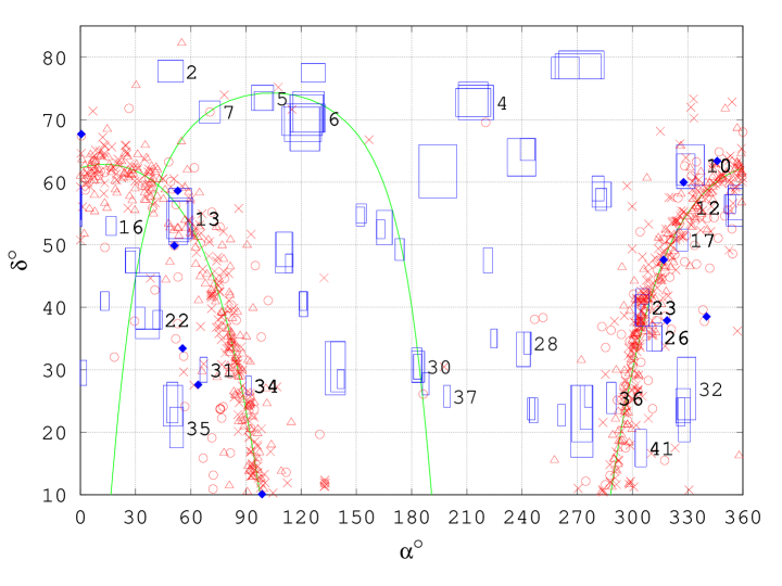
Figure 4: Galactic open clusters and nearby OB-associations. The numbers are shown for the REFs that have open clusters in their 3-degree neighbourhood. Different symbols are used for open clusters located at different distances $d$ from the Solar system: $\circ$ for $d\leq 1$ kpc, $\triangle$ for $1<d\leq 5$ kpc, $\times$ for open clusters at $d>5$ or at unknown distance. Dark diamonds show coordinates of OB-associations out to a distance of 1 kpc from the Solar system.

Notice a number of interesting coincidences. REF 2, which has neither pulsars nor supernova remnants in its vicinity, has two open clusters nearby, namely, Berkeley 8 and SAI 30. They lie far away from the Solar system at the distance $d\approx 3.1$ kpc. Open cluster Collinder 285, which is only out at the distance of 25 pc from the Solar system, is located practically at the southern boundary of REF 4 ($\rho=0.4^{\circ}$). REF 5 also obtains a neighbour with open cluster OCl 374 located at the angular distance $0.65^{\circ}$.

Three REFs have nearby open clusters that are located close to the Solar system. These are Melotte 111 ($d=96$ pc, REF 30), M45 (Pleiades, $d=133$ pc, REF 35) and Melotte 20 ($d=185$ pc, REF 13). Open cluster Platais 3, which lies at the distance of 200 pc from the Solar system, gets almost in the center of REF 7. On the whole, there are open clusters located at distances less than 1 kpc from the Solar system inside or in the close vicinity of 15 regions. Among them, notice a well-known cluster Berkeley 87, located in the Cygnus arm at a distance of 633 pc from the Solar system.

In the vicinity of the REFs, there are a number of OB-associations located close to the Solar system. We mention Cas-Tau association at the distance of 140 pc (REF 31) and $\alpha$ Persei (Per OB3) at the distance of 170 pc (de Zeeuw et al., 1999).

Remark finally that there are no known astrophysical objects of the types considered above in the neighbourhood of REFs 1, 8, 9, 18, 24, 25, 27 and 33.

3 Discussion and Conclusions

We begin the discussion of the presented results with a comparison with results of other experiments. After the first analysis of the data of the EAS MSU array, we pointed out that REFs 4, 5, 6, 10, 11, 12, 16, 17, 22, 30 and 33 practically coincide or have intersecting boundaries with the regions found in the data of the EAS–1000 Prototype array (Zotov, Kulikov, 2009). A small overlapping of the boundaries also had place for REF 8. All these results are confirmed.

There are a number of coincidences with regions of excessive flux of CRs, found in the data obtained with the “Klara-Chronotron” station located in Tian-Shan and aimed to study anisotropy of the cosmic rays at energies $10^{14}$–$10^{15}$ eV (Nesterova et al., 2011). In particular, four regions were found with the statistical significance $>3\sigma$ for a data set that corresponds to the primary energy of protons at around $6\times 10^{14}$ eV. Two of them partially overlap with REFs 6 and 8. Two other are located just near REFs 22 and 39. It is surprising that in the case of REF 8 the overlapping is observed for a region that does not have known possible Galactic sources of PeV CRs nearby. There are also a few coincidences with regions selected with the statistical significance (2.1–3)$\sigma$. REFs 13, 14, 15, 17, 28, 30 and 34 can be listed among them.

As it was already discussed above, a special interest to a search of a small-scale anisotropy of PeV cosmic rays is caused by the recent discoveries of the anisotropy of gamma-rays and CRs with energies in the range from a few units up to several hundred TeV obtained by the Milagro, Tibet AS$\gamma$ and ARGO-YBJ collaborations. It is remarkable that five of eight gamma-ray point sources registered with the Milagro experiment with the statistical significance $>4\sigma$ and located in the part of the celestial sphere considered in the present article (Atkins et al., 2004) are situated in the vicinity of the REFs. Both REFs 23 and 35 have a source inside, one source lies at the angular distance $0.7^{\circ}$ to the south from REF 26, two sources are located at the angular distance $\approx 3^{\circ}$ from (empty!) REF 33. An extended region of TeV gamma-ray emission found later in the Cygnus arm with the statistical significance of $5.5\sigma$ (Saz Parkinson, 2005) also lies inside REF 23. The second after the Crab pulsar brightest Galactic source of TeV gamma-ray emission MGRO J2019+37 (Abdo et al., 2007) is located at the boundary of REF 23.

In addition to the extended region in the Cygnus arm, two other large regions of excessive flux (“Region A” and “Region B”) dubbed as “Milagro hot spots” were found in the Milagro experiment (Abdo et al., 2007, 2008). The regions have an angular size $\gtrsim 10^{\circ}$ and are selected with the statistical significance greater than $12\sigma$. An analysis performed by the Milagro collaboration demonstrated that the source of these regions is an excessive flux of hadrons with energies that correspond to the energy of 10 TeV of a proton. One of the regions is located to the south-west from REF 35. Another one occupies a region approximately between REFs 25 and 29. Similar regions in the energy range from a few TeV up to a few dozen TeV were found in the Tibet AS$\gamma$ (Amenomori et al., 2005, 2006, 2009) and ARGO-YBJ (Di Sciascio, Iuppa, 2011) experiments. In particular, the ARGO-YBJ results show an excessive flux of CRs near REFs 4, 22 and 25. It is interesting that one of the regions of excessive flux of TeV gamma-ray emission registered with the Tibet AS$\gamma$ array with the statistical significance $>4.5\sigma$ is located near empty REF 27.

There are no extended regions of excessive flux in the Tibet AS$\gamma$ data at energies of the order of 300 TeV pronounced as clearly as at lower energies (Amenomori et al., 2006). Still, an analysis of the presented intensity maps reveals a few interesting details. In particular, it happens there is an extended region near the Supergalactic plane around $\alpha\sim 120^{\circ}$, $\delta\sim 70^{\circ}$, i.e., at the place of location of REF 6, which includes subregions with an excess $>4\sigma$.

Up to now, there is no satisfactory model that could explain the origin of the small-scale anisotropy of TeV CRs. The Milagro collaboration and a number of other authors tend to a point of view that the regions found appeared due to a special configuration of magnetic fields and related effects in the heliosphere and at its boundary, or at the adjacent region of the Galaxy at distances within a few dozen parsecs (Drury, Aharonian, 2008; Battaner et al., 2009; Malkov et al., 2010; Amenomori et al., 2010; Giacinti, Sigl, 2011). It is also possible that the anisotropy is caused by the distribution of CRs sources or by propagation effects through the regions of local turbulence generated by the interaction of heliospheric and interstellar magnetic fields (Desiati, Lazarian, 2011). A question whether the models suggested in these works can be extended from TeV energies up to the knee remains open.

If one assumes there are Galactic magnetic fields of the necessary configuration, then there arises a question of their own origin. Another question is why regions of excessive flux are found in the vicinity of some of the possible sources of PeV CRs and are not near the other. Is this due to the properties of these astrophysical objects and the surrounding media or to the properties of the magnetic fields? The questions stated need a special consideration. Since the distances to the pulsars given in Table 3 are much greater than the mean free path of neutrons of PeV energies, and the amount of electro-magnetic showers is not enough to form REFs, there appears a question of how to keep the direction of charged CRs moving through the Galactic magnetic field. One of the possible explanations possibly relates to magnetic lenses.

A classical question of the cosmic ray physics, besides the question of their origin, is their mass composition. In connection with the regions found and the fact that the majority of pulsars in their vicinity can only accelerate sufficiently heavy nuclei to PeV energies, it is interesting to note that the analysis of the Tibet AS$\gamma$ data lead to a conclusion that these are not protons that dominate in the region of the knee but nuclei heavier than helium (Amenomori, 2006b, 2008). A similar conclusion was made basing on the data obtained at mount Chacaltaya (Tokuno et al., 2008).

We believe the results of the present research together with our earlier works allow us to make a conclusion that there exists a small-scale anisotropy of cosmic rays with energies at around PeV and a typical angular size from $3^{\circ}$ up to $12^{\circ}$. Location of a considerable number of the regions of excessive flux on the celestial sphere correlates with coordinates of the Galactic SNRs, pulsars, OB-associations and open clusters. In our opinion, the correlation of REFs with multiple potential sources of PeV CRs can witness that Galactic cosmic rays registered on Earth were not born in a single source but in many astrophysical sources of different nature. Questions of how to preserve a direction of movement of CRs from their sources to Earth in case these astrophysical objects give birth to the REFs, and how to explain the regions without any known possible sources of CRs in their neighbourhood, remain open and their solution probably needs more detailed information on the structure of the interstellar magnetic field in the vicinity of the Solar system.

Only free, open source software was used for the investigation. In particular, all calculations were performed with GNU Octave running in Linux. The research has made use of the SIMBAD database, operated at CDS, Strasbourg, France (http://simbad.u-strasbg.fr/simbad).

The research was partially supported by the Russian Foundation for Fundamental Research grant No. 11-02-00544 and Federal contract No. 16.518.11.7051.

References

- [1] R. Abbasi, Y. Abdou, T. Abu-Zayyad, et al., Astrophys. J. 740, 16 (2011); arXiv:1105.2326v4.
- [2] R. Abbasi, Y. Abdou, T. Abu-Zayyad, et al., Observation of an Anisotropy in the Galactic Cosmic Ray arrival direction at 400 TeV with IceCube, arXiv:1109.1017v1.
- [3] A.A. Abdo, B. Allen, D. Berley, et al., Astrophys. J. 658, L33 (2007); arXiv:astro-ph/0611691v1.
- [4] A.A. Abdo, B. Allen, T. Aune, et al., Phys. Rev. Lett. 101, 221101 (2008); arXiv:0801.3827v3.
- [5] A.A. Abdo, B.T. Allen, T. Aune, et al., Astrophys. J. Lett. 700, L127 (2009); arXiv:0904.1018.
- [6] A.A. Abdo, M. Ackermann, M. Ajello, et al., Fermi Large Area Telescope Second Source Catalog, arXiv:1108.1435v1.;
- [7] M. Ackermann, M. Ajello, A. Allafort, et al., Science 334, 1103 (2011).
- [8] D.E. Alexandreas, D. Berley, S. Biller, et al., Astrophys. J. 383, L53 (1991).
- [9] M. Amenomori, S. Ayabe, D. Chen, et al., Astrophys. J. 633, 1005 (2005).
- [10] M. Amenomori, S. Ayabe, X.J. Bi, et al., Science 314, 439 (2006); arXiv:astro-ph/0610671.
- [11] M. Amenomori, S. Ayabe, D. Chen, et al., Phys. Lett. B 632, 58 (2006); arXiv:astro-ph/0511469.
- [12] M. Amenomori, S. Ayabe S., X.J. Bi, et al., Nucl. Phys. B (Proc. Suppl.) 175–176, 318 (2008).
- [13] M. Amenomori, X.J. Bi, D. Chen, Large-scale sidereal anisotropy of multi-TeV galactic cosmic rays and the heliosphere, arXiv:0909.1026.
- [14] M. Amenomori and The Tibet AS Collaboration, Astrophys. Space Sci. Trans. 6, 49 (2010).
- [15] D. Andrews, A.C. Evans, R.J.O. Reid, et al., Proc. 11th ICRC, Budapest, Hungary, 1969 (Acta Physica 29, Suppl. 3, (1970)), p. 343.
- [16] Z. Arzoumanian, E.V. Gotthelf, S.M. Ransom, et al., Discovery of an Energetic Pulsar Associated With SNR G76.9+1.0, arXiv:11053185v1.
- [17] R. Atkins, W. Benbow, D. Berley, et al., Astrophys. J. 608, 680 (2004); arXiv:atsro-ph/0403097.
- [18] E. Battaner, E. Castellano, M. Masip, Astrophys. J. Lett. 703, L90 (2009); arXiv:0907.2889v2.
- [19] A. Bhadra, Proc. 28th ICRC. Tsukuba, Japan (Ed. T. Kajita, Y. Asaoka, A. Kawachi, Y. Matsubara and M. Sasaki, 2003), p. 303.
- [20] A. Bhadra, Astropart. Phys. 25, 226 (2006); arXiv:astro-ph/0602301.
- [21] W.R. Binns, M.E. Wiedenbeck, M. Arnould, et al., New Astronomy Reviews 52, 427 (2008).
- [22] P. Blasi, R.I. Epstein, A.V. Olinto, Astrophys. J. 533, L123 (2000); arXiv:astro-ph/9912240.
- [23] A.M. Bykov, V.S. Ptuskin, I.N. Toptygin, Proc. 24th ICRC, Rome, Italy (Ed. N. Iucci, E. Lamanna, 1995, vol. 3), p. 337.
- [24] P. Desiati and A. Lazarian, Anisotropy of TeV Cosmic Rays and the Outer Heliospheric Boundaries, arXiv:1111.3075v1.
- [25] W.S. Dias, B.S. Alessi, A. Moitinho, et al., Astron. Astrophys. 389, 871 (2002). http://www.astro.iag.usp.br/~wilton/; updated Nov. 24, 2010.
- [26] G. Di Sciascio and R. Iuppa, Proc. 32nd ICRC, Beijing, China (2011, vol. 1), p. 74.
- [27] L.O’C. Drury and F.A. Aharonian, Astropart. Phys. 29, 420 (2008); arXiv:0802.4403v2.
- [28] A.D. Erlykin and A.W. Wolfendale, Are there pulsars in the knee?, arXiv:astro-ph/0408225.
- [29] G. Giacinti and G. Sigl, Local Magnetic Turbulence and TeV-PeV Cosmic Ray Anisotropies, arXiv:1111.2536v1.
- [30] M. Giller and M. Lipski, J. Phys. G 28, 1275 (2002).
- [31] A. Giuliani, M. Cardillo, M. Tavani, et al., Astrophys. J. 742, L30 (2011); arXiv:1111.4868v1.
- [32] D.A. Green, Bull. of the Astron. Soc. of India 37, 45 (2009); arXiv:0905.3699. http://www.mrao.cam.ac.uk/surveys/snrs/
- [33] G. Guillian, J. Hosaka, K. Isihara, et al., Phys. Rev. D 75, 062003 (2007); arXiv:astro-ph/0508468v4.
- [34] J.E. Gunn and J.P. Ostriker, Phys. Rev. Lett. 22, 728 (1969).
- [35] J.P. Halpern, Is Calvera a Gamma-Ray Pulsar?, arXiv:1106.2140v1.
- [36] J.C. Higdon and R.E. Lingenfelter, Astrophys. J. 628, 738 (2005).
- [37] A.M. Hillas, J. Phys. G 31, R95 (2005).
- [38] B. Jiang, Y. Chen, J. Wang, et al., ApJ 712, 1147 (2010).
- [39] G.V. Kulikov and M.Yu. Zotov, A search for outstanding sources of PeV cosmic rays: Cassiopeia A, the Crab Nebula, the Monogem Ring–But how about M33 and the Virgo cluster?, arXiv:astro-ph/0407138.
- [40] M.A. Malkov, P.H. Diamond, L.O’C. Drury, et al., Astrophys. J. 721, 750 (2010); arXiv:1005.1312v2.
- [41] R.N. Manchester, G.B. Hobbs, A. Teoh, et al., Astrophys. J. 129, 1993 (2005). The ATNF Pulsar Database, http://www.atnf.csiro.au/research/pulsar/psrcat/
- [42] G. Morlino and D. Caprioli, Strong evidences of hadron acceleration in Tycho’s Supernova Remnant, arXiv:1105.6342v2.
- [43] A. Neronov and D. V. Semikoz, Origin of TeV Galactic Cosmic Rays, arXiv:1201.1660v1.
- [44] N.M. Nesterova, A. Varga, E.N. Gudkova, et al., Izvestiya RAN, ser. fiz. 75, 368 (2011).
- [45] Y. Oyama, Anisotropy of the primary cosmic-ray flux in Super-Kamiokande, arXiv:astro-ph/0605020v2.
- [46] E. Parizot, A. Marcowith, E. van der Swaluw, et al., Astron. Astrophys. 424, 747 (2004); arXiv:astro-ph/0405531.
- [47] N. Prantzos, On the origin and composition of Galactic cosmic rays, arXiv:1112.4343v1.
- [48] V. Ptuskin, V. Zirakazhvili, E.-S. Seo, Astrophys. J. 718, 31 (2010); arXiv:1006.0034.
- [49] M.J. Reid, J.E. McClintock, R. Narayan, et al., The Trigonometric Parallax of Cygnus X-1, arXiv:1106.3688v1.
- [50] P.M. Saz Parkinson, Recent results from the Milagro TeV gamma-ray observatory, arXiv:astro-ph/0505335v1.
- [51] K. Suga, H. Sakuyama, S. Kawaguchi, et al., Phys. Rev. Lett. 27, 1604 (1971).
- [52] H. Tokuno, F. Kakimoto, S. Ogio, et al., Astropart. Phys. 29, 453 (2008).
- [53] S.N. Vernov, G.B. Khristiansen, V.B. Atrashkevich, et al., Proc. 16th ICRC. V. 8. Kyoto (Ed. Saburo Miyake, Institute for Cosmic Ray Research, University of Tokyo, 1979), p. 129.
- [54] P.T. de Zeeuw, R. Hoogerwerf, J.H.J. de Bruijne, et al., Astron. J. 117, 354 (1999); arXiv:astro-ph/9809227.
- [55] M.Yu. Zotov and G.V. Kulikov, Izvestiya RAN, ser. fiz. 68, 1602 (2004).
- [56] M.Yu. Zotov and G.V. Kulikov, Bull. Russ. Acad. Sci.: Physics 71, 483 (2007); arXiv:astro-ph/0610944.
- [57] M.Yu. Zotov and G.V. Kulikov, Izvestiya RAN, ser. fiz. 73, 612 (2009); arXiv:0902.1637.
- [58] M.Yu. Zotov and G.V. Kulikov, Astron. Lett. 36, 645 (2010); arXiv:0907.3192.
- [59] M.Yu. Zotov and G.V. Kulikov, Bull. Rus. Acad. Sci., Physics 75, 342–346 (2011); arXiv:1107.2784.