Jaynes-Cummings model: What emerges first beyond the rotating-wave approximation?

Abstract

The Jaynes-Cummings model without the rotating-wave approximation can be solved exactly by extended Swain’s ansatz with the conserved parity. The analytical approximations are then performed at different levels. The well-known rotating-wave approximation is naturally covered in the present zero and first approximations. The effect of the counter rotating-wave term emerges clearly in the second order approximation. The concise analytical expressions are given explicitly and can be applicable up to the ultra-strong coupling regime. The preliminary application to the vacuum Rabi splitting is shown to be very successful.

I introduction

The interaction of light with matter is a fundamental one in optical physics. The simplest paradigm is a two-level atom coupled to the electromagnetic mode of a cavity. In the strong coupling regime where the coupling strength $g/\omega$ ($\omega$ is the cavity frequency) between the atom and the cavity mode exceeds the loss rates, the atom and the cavity can repeatedly exchange excitations before coherence is lost. The Rabi oscillations can be observed in this strong coupling atom-cavity system, which is usually called as cavity quantum electrodynamics (QED) CQED . Typically, the coupling strength in cavity QED reaches $g/\omega\thicksim 10^{-6}$. It can be described by the well-known Jaynes-Cummings (JC) modelJC .

Recently, for superconducting qubits, a one-dimensional (1D) transmission line resonatorWallraff or a LC circuitChiorescu ; Wang ; Deppe can play a role of the cavity, which is known today as circuit QED. More recently, LC resonator inductively coupled to a superconducting qubitNiemczyk ; exp ; Mooij has been realized experimentally. The qubit-resonator coupling has been strengthened from $g/\omega\thicksim 10^{-3}$ in the earlier realizationWallraff , a few percentage later Fink ; Deppe , to most recent ten percentagesNiemczyk ; exp ; Mooij . In cavity QED system, the rotating-wave approximation (RWA) is usually made, however, in the circuit QED, due to the ultra-strong coupling strength $g/\omega\thicksim 0.1$ Niemczyk ; exp ; Mooij , evidence for the breakdown of the RWA has been providedNiemczyk . Therefore, counter rotating-wave terms (CRTs) in the JC model should be included. Recently, many works have been devoted to this qubit-oscillator system in the ultra-strong coupling regimeWerlang ; Hanggi ; Nori ; Hwang; Hausinger ; chen10b .

Actually, the JC model without the RWA has been studied extensively for more than 40 years. A incomplete list is given by Refs. Swain ; Kus ; Durstt ; Tur ; Bishop ; Feranchuk ; Liu1 ; Irish ; chenqh ; liu ; chen10 ; Pan ; Casanova ; QingHu1 . Two main schemes are employed. One is based on the photonic Fock statesSwain ; Kus ; Durstt ; Tur ; Feranchuk ; Bishop with the pioneer work by SwainSwain . The continued fractions are present and the solution ten becomes very intricate. The other is on the basis of various polaron-like transformations or shifted operators, which are basically photonic coherent states approachesLiu1 ; Irish ; chenqh ; liu ; chen10 ; Pan ; Casanova ; QingHu1 . The very accurate solution can be obtained readily, but the infinite photonic Fock states should be involved.

The RWA eigenstates only include two bare states, which have facilitated earlier clean investigations on various quantum phenomena in quantum optics. Surprisingly, one or a few dominant terms in the eigenstates of the JC Hamiltonian beyond the RWA ones are still lacking or not given explicitly until now, to the best of our knowledge. What emerges first beyond the RWA results may be very useful to analyze the effect of CRTs on various phenomena at the microscopic level. In this sense, a few dominant terms are more helpful than the exact solution including infinite bare states.

In this paper, by using the conserved parity, we extend Swain’s wavefunction to the JC model without the RWA. We will not follow the usual exact diagonalization routine. Alternatively, we derive a polynomial equation with only single variable, just the eigenvalue that we seek. The solutions to this polynomial equation can give exactly all eigenfunctions and eigenvalues for arbitrary parameters. Moveover, we can perform approximations step by step with the help of these exact solutions. The zero and first order approximations will exactly recover the RWA results. The dominant effect of the CRTs emerges in the second order approximation.

Without the RWA, the Hamiltonian of a two-level atom (qubit) with transition frequency $\Delta$ interacting with a single-mode quantized cavity of frequency $\omega$ is

$$H=\frac{\Delta}{2}\sigma_{z}+\omega a^{\dagger}a+g\left(a^{\dagger}+a\right)\sigma_{x},$$ (1)

where $g$ is coupling strength. $\sigma_{x}$ and $\sigma_{z}$ are Pauli spin-$1/2$ operators, $a^{\dagger}$ and $a$ are the creation and annihilation operators for the quantized field. Here, $\delta=\Delta-\omega$ is defined as the dimensionless detuning parameter. The energy scale is set $\omega=1\;$here.

The RWA is made by neglecting the CRTs, $a^{\dagger}\sigma_{+}+a\sigma_{-}$, then one can easily diagonalize the Hamiltonian and obtain the eigenfunctions asScully

$$\left|{}\right\rangle^{RWA}=\left(\ \begin{array}[]{l}c_{n}\left|n\right\rangle\\ d_{n}\left|n+1\right\rangle\end{array}\right),n=0,1,2,...$$ (2)

For later use, we also list the relevant eigenvalues

$$E_{1n}^{RWA} = n+\frac{1}{2}-\frac{1}{2}R_{n},$$ (3)

$$E_{2n}^{RWA} = n+\frac{1}{2}+\frac{1}{2}R_{n},$$ (4)

where $R_{n}=\sqrt{\delta^{2}+4g^{2}\left(n+1\right)}$. In the ground state (GS), the qubit is in GS and the photon is in a vacuum state. The GS energy is $E^{0}=-\frac{\Delta}{2}$.

Associated with JC Hamiltonian with and without the RWA is a conserved parity $\Pi$, such that $\left[H,\Pi\right]=0$, which is given by

$$\Pi=\sigma_{x}\exp\left(i\pi\widehat{N}\right),$$ (5)

where $\widehat{N}=$ $a^{+}a$ is the bosonic number operator. $\Pi$ has two eigenvalues $\pm 1$, depending on whether the excitation number is even or odd. The above two states (6) and (7) with even $n$ are of odd parity and with odd $n$ even parity. The ground state is of even parity. The RWA results for the first $8$ energy levels at resonance, $E_{1(2)n}=n+\frac{1}{2}\pm g\sqrt{n+1)}$, are given in Fig. 1 (a) for later comparisons.

II Exact solution without the RWA

First we introduce a scheme to obtain the exact solutions to the JC model without the RWA. For convenience, we can write a transformed Hamiltonian with a rotation around an $y$ axis by an angle $\frac{\pi}{2}$. In the Matrix form it takes

$$H=\left(\begin{array}[]{ll}a^{\dagger}a+g(a^{\dagger}+a)-\alpha&-\frac{\Delta}{2}\\ -\frac{\Delta}{2}&a^{\dagger}a-g(a^{\dagger}+a)\end{array}\right).$$ (6)

About 40 years ago, Swain first proposed an ansatz for the wavefunction in the photonic Fock statesSwain , which is also a starting point of the standard numerically exact diagonalization (ED) scheme. Since then, various methods have been developed along this line Kus ; Durstt ; Tur ; Bishop , but the conserved parity has not been considered, to our knowledge. Therefore continued fractions are unavoidably presented in the expressions for the eigensolutions.

We also proceed along this line, but the parity is incorporated in the Swain’s ansatz, which is given by

$$\left|{}\right\rangle=\left(\ \begin{array}[]{l}\sum_{n=0}^{M}c_{n}\left|n\right\rangle\\ \pm\sum_{n=0}^{M}(-1)^{n}c_{n}\left|n\right\rangle\end{array}\right)$$ (7)

with $+(-)$ stands for even (odd) parity, M is the truncated number. The Schr$\stackrel{{\scriptstyle..}}{{o}}$dinger equation gives

$$\sum_{n=0}a^{\dagger}ac_{n}\left|n\right\rangle+g\sum_{n=0} c_{n} \left(\sqrt{n}\left|n-1\right\rangle+\sqrt{n+1}\left|n+1\right\rangle\right)$$

$$\mp\frac{\Delta}{2}\sum_{n=0}(-1)^{n}c_{n}\left|n\right\rangle = Ec_{n}\left|n\right\rangle.$$ (8)

Left multiplying the photonic states $\left\langle m\right|$ gives

$$mc_{m}+g\sqrt{m+1}c_{m+1}+g\sqrt{m}c_{m-1}\mp\frac{\Delta}{2}(-1)^{m}c_{m}=Ec_{m},$$

then we have a recurrence relation

$$c_{m+1}=\frac{1}{g\sqrt{m+1}}\left[E-m\pm\frac{\Delta}{2}(-1)^{m}\right]c_{m}-\sqrt{\frac{m}{m+1}}c_{m-1}.$$ (9)

By careful inspection of Eq. (7), one can find that $c_{0}$ is flexible in the Schr$\stackrel{{\scriptstyle..}}{{o}}$dinger equation where the normalization for the eigenfunction is not necessary, so we select $c_{0}=1.0$. Then we have

$$c_{1}=\frac{1}{g}\left[E\pm\frac{\Delta}{2}\right].$$

Once the first two terms are fixed, the coefficients of the other terms higher than $a^{+}$ should be determined by the recurrence relation Eq. (9)

For $m=M$, the terms higher then $\left(a^{+}\right)^{M}$ are neglected, we may set $c_{M+1}=0$, then we have

$$\left[E-M\pm\frac{\Delta}{2}(-1)^{M}\right]c_{M}-g\sqrt{M}c_{M-1}=0.$$ (10)

Note that this is actually a one-variable polynomial equation of degree $M$. The variable is just the eigenvalue we want to obtain. It is expected that the roots of Eq. (10) would give the exact solutions to the JC model without the RWA if M is large enough.

To obtain the true exact results, in principle, the truncated number $M$ should be taken to infinity. Fortunately, it is not necessary. It is found that finite terms in state (7) are sufficient to give exact results in the whole coupling range. The usual numerical exact diagonalization can readily give the energy levels and their wavefunctions in the JC model, which can be regarded as a benchmark. We will increase the truncated number $M$ until the relative difference of the energies obtained from the roots and the standard value is just less than $10^{-7}$, which sets the criterion for the convergence achieved. Interestingly, for coupling constant $g\leq 0.1$ for three typical atom frequency $\Delta=0.1,1$, and $1.5$, the truncated number $M=15$ in the polynomial equation can give exactly $20$ energy levels by the above criterion for convergence. For $g=1.0$ and $2.0$, the polynomial equations with $M=25$ and $40$ can yield about $20$ energy levels exactly. In fact, all above calculations can be immediately done in an ordinary PC.

Figure 1: The first 8 energy levels as a function of coupling constant $g$ at resonance. The exact results without the RWA are presented by black solid line. (a) The RWA results (red dashed line) and (b) The analytical results in Eqs. (26), (27), (34), and (36) of the second-order approximation (red dashed line).

For late use, the first 8 exact energy levels as a function of the coupling constant $g$ obtained by the above polynomial equations with $M=25$ at resonate case ($\Delta=1$) are presented in Fig. 1(a) and (b) by black solid lines. The parity is not changed after the level crossing.

We then try to follow the energy curves to get some analytical approximate results in the next section.

III Analytical results without RWA

The recurrence relation Eq. (9) can be simplified to a tridiagonal form

$$\left(\begin{array}[]{lllll}\Omega_{0}(E)&1&0&...&0\\ 1&\Omega_{1}(E)&\sqrt{2}&...&0\\ 0&\sqrt{2}&\Omega_{2}(E)&...&0\\ \ ...&\ ...&...&...&...\\ 0&0&0&\sqrt{M}&\Omega_{M}(E)\end{array}\right)\left(\begin{array}[]{l}c_{0}\\ c_{1}\\ c_{2}\\ ...\\ c_{M}\end{array}\right)=0,$$

where

$$\Omega_{m}(E)=\frac{1}{g}\left[m-E\mp\frac{\Delta}{2}(-1)^{m}\right].$$ (11)

The eigensolutions can be obtained from the zeros of the determinant of the Matrix,

The zero-order approximation $\Omega_{m}(E)=0\;$gives

$$E^{m}=m\mp(-1)^{m}\frac{\Delta}{2}.$$

The lowest energy is

$$E^{0}=-\frac{\Delta}{2}.$$

The ground-state is of even parity, so the state is

$$\left|0\right\rangle^{{}^{\prime}}=\left(\ \begin{array}[]{l}c_{0}\left|0\right\rangle\\ c_{0}\left|0\right\rangle\end{array}\right).$$ (12)

Transforming back to the original frame gives

$$\left|0\right\rangle=\frac{1}{\sqrt{2}}\left(\begin{array}[]{ll}1&-1\\ 1&1\end{array}\right)\left(\ \begin{array}[]{l}c_{0}\left|0\right\rangle\\ c_{0}\left|0\right\rangle\end{array}\right)\varpropto\left|g,0\right\rangle,$$

Interestingly, the first element in the zero-order approximation actually gives exactly the ground-state in the RWA. The other solutions are $g$ irrelevant and therefore omitted.

III.1 The first approximation

The first approximation is made by selecting the matrices with two order along the diagonal line

$$\left(\begin{array}[]{ll}\Omega_{m}(E)&\sqrt{m+1}\\ \sqrt{m+1}&\Omega_{m}(E)\end{array}\right)\left(\begin{array}[]{l}c_{m}\\ c_{m+1}\end{array}\right)=0.$$ (13)

It is expected that the $m-th$ two order determinant would contain the information of the two levels with same parity. Comparing with the RWA results, it can be inferred that even $m$ is corresponding to odd parity and odd $m$  to the even parity. Fortunately, we have the same $\Omega(E)$ for any value of $m$

$$\Omega_{m}(E)=\frac{1}{g}\left[m-E+\frac{\Delta}{2}\right].$$

Then we have following quadratic equation

$$\left(m-E+\frac{\Delta}{2}\right)\left(m+1-E-\frac{\Delta}{2}\right)-\left(m+1\right)g^{2}=0,$$

which yields the eigenvalues

$$E=m+\frac{1}{2}\pm\frac{1}{2}\sqrt{\left(1-\Delta\right)^{2}+4g^{2}\left(m+1\right)}.$$ (14)

They are just the RWA ones in Eqs. (3) and (4) .

According to the wavefunction Eq. (7), the eigenstate is then obtained as

$$\left|m\right\rangle^{\prime}=\left(\ \begin{array}[]{l}c_{m}\left|m\right\rangle+c_{m+1}\left|m+1\right\rangle\\ \pm(-1)^{m}\left[c_{m}\left|m\right\rangle-c_{m+1}\left|m+1\right\rangle\right]\end{array}\right).$$ (15)

By the above relation between $m\;$and parity, we always have $\pm(-1)^{m}=-1.$ Transforming back to the original frame gives

$$\left|m\right\rangle=\frac{1}{\sqrt{2}}\left(\begin{array}[]{ll}1&-1\\ 1&1\end{array}\right)\left|m\right\rangle^{\prime}\varpropto\left(\ \begin{array}[]{l}c_{m}\left|m\right\rangle\\ c_{m+1}\left|m+1\right\rangle\end{array}\right),$$ (16)

which are just the eigenstates under the RWA in Eq. (2) for excited states.

So in the first approximation, we can not obtained results more than the RWA ones for all excited states. The effect of the CRTS should only emerges beyond the first approximation.

III.2 The second order approximation

Naturally, the second order approximation is performed by reducing to the $m-th$ three order determinant as

$$\left|\begin{array}[]{lll}\Omega_{m}(E)&\sqrt{m+1}&0\\ \sqrt{m+1}&\Omega_{m+1}(E)&\sqrt{m+2}\\ 0&\sqrt{m+2}&\Omega_{m+2}(E)\end{array}\right|=0.$$ (17)

For more concise, we only consider the resonant case $\delta=0$. It is straightforward to extend to finite detunings.

Two univariate cubic equations for even and odd parity can be explicitly derived for any $m-th$ three order determinant. Three roots $y_{1}<y_{2}<y_{3}$ for each univariate cubic equation can be obtained easily by the formula presented in the Appendix A. Comparing with the exact ones obtained above, one can find that the second roots $y_{2}$ are the true solutions. Especially, the first root $y_{1}$ for $m=0$ with even (odd) parity gives the energy in the GS (the first excited state). With these results in mind, the general solutions can be grouped as the following two cases, and all eigenvalues and eigenfunctions can be given analytically in the unified way.

III.2.1 $m=2k$ with even parity and $m=2k+1$ with odd parity

For both $m=2k$ with even parity and $m=2k+1$ with odd parity ($k=0,1,2,...$ ), we have the same univariate cubic equation in the following form

$$E^{3}-\left(3m+\frac{5}{2}\right)E^{2}$$

$$+\left[\left(m+\frac{3}{2}\right)\left(3m+\frac{1}{2}\right)-\left(2m+3\right)g^{2}\right]E$$

$$-\allowbreak\left(m-\frac{1}{2}\right)\left(m+\frac{3}{2}\right)^{2}+\left[2m^{2}+4m+\frac{1}{2}\right]g^{2}=0.$$ (18)

According to the Appendix A, we have

$$A = 4+\allowbreak\left(6m+9\right)g^{2},$$

$$B = -8m-12-\allowbreak\left(12m^{2}+22m-3\right)g^{2},$$

$$C = \allowbreak\left(2m+3\right)^{2}g^{4}+\left(6m^{3}+13m^{2}+\frac{3}{2}m-\frac{3}{4}\right)g^{2}$$

$$+\allowbreak 4m^{2}+12m+9.$$

It can be readily proven $\Gamma=B^{2}-4AC<0\;$in this case, so there are three different real roots. Note above that the energy level is given by the second root $y_{2}$, so

$$E=\frac{\left(3m+\frac{5}{2}\right)+\sqrt{4+\allowbreak\left(6m+9\right)g^{2}}\left[\cos\theta-\sqrt{3}\sin\theta\right]}{3},$$ (19)

with

$$\theta=\frac{1}{3}\arccos\left(\frac{\allowbreak 8-\left(9m+27\right)g^{2}}{\sqrt{\left[4+\allowbreak\left(6m+9\right)g^{2}\right]^{3}}}\right).$$

Especially, $m=0$ with even parity will give the GS additionally. The GS energy is given by the first root $y_{1}$

$$E_{GS}=\frac{\frac{5}{2}+\sqrt{4+\allowbreak 9g^{2}}\left[\cos\theta+\sqrt{3}\sin\theta\right]}{3},$$ (20)

with

$$\theta=\frac{1}{3}\arccos\left(\frac{\allowbreak 8-27g^{2}}{\sqrt{\left(4+\allowbreak 9g^{2}\right)^{3}}}\right).$$

The states in this case all takes the form

$$\left|{}\right\rangle\varpropto\left(\ \begin{array}[]{l}c_{m+1}\left|m+1\right\rangle\\ c_{m}\left|m\right\rangle+c_{m+1}\left|m+2\right\rangle\end{array}\right).$$ (21)

III.2.2 $m=2k+1$ with even parity and $m=2k\$ with odd parity

For both $m=2k+1$ with even parity and $m=2k\$ with odd parity, we have the same univariate cubic equation in the other form

$$E^{3}-\left(3m+\frac{7}{2}\right)E^{2}$$

$$+\left[\left(m+\frac{1}{2}\right)\left(3m+\frac{11}{2}\right)-\left(2m+3\right)g^{2}\right]E$$

$$-\left(m+\frac{1}{2}\right)^{2}\left(m+\frac{5}{2}\right)+\left(2m^{2}+6m+\frac{7}{2}\right)g^{2}=0.$$ (22)

Similarly, we have

$$A = \left(6m+9\right)g^{2}+4,$$

$$B = \allowbreak\left(-12m^{2}-38m-21\right)g^{2}+\allowbreak\left(-8m-4\right),$$

$$C = \allowbreak\left(-2m-3\right)^{2}g^{4}+\left(6m^{3}+29m^{2}+\frac{83}{2}m+\frac{81}{4}\right)g^{2}$$

$$+4m^{2}+4m+1.$$

One can also readily prove $\Gamma=B^{2}-4AC<0$, So there are also three different real roots. The energy level is given by the second root$\;y_{2}$,

$$E=\frac{\left(3m+\frac{7}{2}\right)+\sqrt{\left(6m+9\right)g^{2}+4}\left[\cos\theta-\sqrt{3}\sin\theta\right]}{3},$$ (23)

with

$$\theta=\frac{1}{3}\arccos\left(\frac{-8+9mg^{2}}{\sqrt{\left[4+\left(6m+9\right)g^{2}\right]^{3}}}\right).$$

Especially, $m=0$ with odd parity will yield the first excited state additionally. The corresponding eigenenergy is given by the first root $y_{1}$

$$E_{1}=y_{1}=\frac{\frac{7}{2}+\sqrt{9g^{2}+4}\left[\cos\theta+\sqrt{3}\sin\theta\right]}{3},$$ (24)

with

$$\theta=\frac{1}{3}\arccos\left(\frac{-8}{\sqrt{\left(4+9g^{2}\right)^{3}}}\right).$$

The states in this case all takes the form

$$\left|{}\right\rangle\varpropto\left(\ \begin{array}[]{l}c_{m}\left|m\right\rangle+c_{m+2}\left|m+2\right\rangle\\ c_{m+1}\left|m+1\right\rangle\end{array}\right).$$ (25)

III.2.3 Unified expressions

For the future use, we will give the unified expression of the eigenvalues and eigenfucntions, which are corresponding to those in the RWA one by one in the following.

Set $m=n-1$ in II B(1) and $m=n$ in II B(2), the eigenvalues in Eqs. (19) and (23) can be expanded in terms of $g$ as

$$E_{1n} = n+\frac{1}{2}-g\sqrt{n+1}$$ (26)

$$+\frac{n}{4}g^{2}+\frac{1}{32}\frac{\left(3n+4\right)n}{\sqrt{n+1}}g^{3}+...$$

$$E_{2n} = n+\frac{1}{2}+g\sqrt{n+1}$$ (27)

$$-\frac{\left(n+2\right)}{4}g^{2}-\frac{1}{32}\frac{\left(n+2\right)\left(3n+2\right)}{\sqrt{n+1}}g^{3}+...$$

The corresponding eigenstates take the form

$$\left|1n\right\rangle \varpropto \left(\ \begin{array}[]{l}c_{n}\left|n\right\rangle\\ \left(c_{n-1}\left|n-1\right\rangle+c_{n+1}\left|n+1\right\rangle\right)\end{array}\right),$$ (30)

$$\left|2n\right\rangle \varpropto \left(\ \begin{array}[]{l}c_{n}\left|n\right\rangle+c_{n+2}\left|n+2\right\rangle\\ c_{n+1}\left|n+1\right\rangle\end{array}\right).$$ (33)

It should be pointed out that the GS state and the first excited state can not be brought into the above general expression for $n=0$. The GS energy and the GS state with even parity are

$$E_{GS}=-\frac{1}{2}-\frac{1}{2}g^{2}-\frac{1}{8}g^{4}+...$$ (34)

$$\left|GS\right\rangle\varpropto\left(\ \begin{array}[]{l}c_{1}\left|1\right\rangle\\ \left(c_{0}\left|0\right\rangle+c_{2}\left|2\right\rangle\right)\end{array}\right),$$ (35)

and the first excited state with odd parity are

$$E_{1}=\frac{1}{2}-g-\frac{1}{2}g^{2}+\frac{1}{8}g^{3}+...$$ (36)

$$\left|1EX\right\rangle\varpropto\left(\ \begin{array}[]{l}c_{0}\left|0\right\rangle+c_{2}\left|2\right\rangle\\ c_{1}\left|1\right\rangle\end{array}\right).$$ (37)

In any case, the ratios of coefficients in the second approximation are

$$c_{m}:c_{m+1}:c_{m+2}=\left[-\frac{\sqrt{m+1}}{\Omega_{m}(E)}\right]:1:\left[-\frac{\sqrt{m+2}}{\Omega_{m+2}(E)}\right],$$ (38)

where the sign $\mp\;$in Eq. (11) for $\Omega_{m}(E)\;$ for any eigenstates is only parity dependent.

It is interesting to note that the first two terms in Eqs. (26), (27) are no other than the RWA results by Eqs. (3) and (4) at resonance. The additional terms appear just because of the presence of the CRTs. Also the eigenfunctions in Eqs. (30) and (33) contain the components of the RWA ones in Eq. (2). The other bare state which can not be generated by the rotating-wave terms also emerges. This is just our answer to the question presented in the title of this paper.

The analytical results for the energy levels in the second order approximation are collected in Fig. 1(b) with red lines. It is shown that for $g\leq 0.4$, the present second order approximation can give reasonable good results. More over, it should be deeply impressed that analytical expressions are almost exact for remarkable wide coupling regime $g\leq$ 0.2. So it could become a solid and concise platform to discuss the effect of CRTs on various physical phenomena in the present experimentally accessible systems. Note that the present maximum value for the coupling strength in the superconducting qubit coupled to a circuit resonant Niemczyk has reached $g=0.12$, to our knowledge. The application to the Vacuum Rabi splitting is performed in the next section as a first example.

IV Vacuum Rabi splicings

If we pump the dressed atom from its ground to an excited state, it will decay to the dressed ground state through spontaneous emissions. Under the RWA, when the atom is excited by the operator, $V=|e\rangle\langle g|+|g\rangle\langle e|$, from the ground state $|g,0>$ , the emission spectrum has two peaks with equal height. The distance of the two peaks, $2g$, is just the vacuum Rabi splitting  agarwal ; Thompson .

Without the RWA, we have two choices for the initial states. When the CRTs are included, the photon in the ground state are no longer a vacuum state, as shown in Eq. (35). In the framework of the second order approximation, we first use $V$ to excite the atom from the ground state at resonance

$$\left|VRS\right\rangle^{(1)}=V\left|GS\right\rangle\varpropto\left(\ \begin{array}[]{l}c_{0}\left|0\right\rangle+c_{2}\left|2\right\rangle\\ c_{1}\left|1\right\rangle\end{array}\right),$$

which can be expanded in terms of the eigenstates with odd parity. Note that only the following 4 excited states are included

$$\left|VRS\right\rangle^{(1)}=v_{1}\left|1EX\right\rangle+v_{2}\left|2EX\right\rangle+v_{5}\left|5EX\right\rangle+v_{6}\left|6EX\right\rangle.$$ (39)

The probabilities $h_{i}=\left|\nu_{i}\right|^{2}$ can be expressed in $g\;$as

$$h_{1} = \frac{1}{2}+\frac{1}{4}g+\frac{11}{32}g^{3}-\frac{1}{16}g^{4}+...$$

$$h_{2} = \frac{1}{2}-\frac{1}{4}g-\frac{11}{32}g^{3}-\frac{1}{16}g^{4}+...$$

$$h_{3} = \frac{3}{64}g^{6}+...$$

$$h_{4} = \frac{1}{16}g^{4}+\frac{\sqrt{3}}{48}g^{5}+...$$

The atom will decay from the initial state to the dressed ground state with an emission spectrum. The heights of the peaks in the spectrum are proportional to the square of the probability of the corresponding eigenstates. Therefore one may find two main peaks, and the other two peaks are too small to be visible, by the above $4$ probabilities.

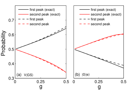
Figure 2: (Color online) The peak heights (dashed lines) in emission spectrum as a function of coupling constant at resonance for the initial states (a) $V\left|GS\right\rangle^{\prime}$ and (b)$|e,0>$. The exact results are marked by black line, the present analytical results by dashed lines.

In Fig. 2 (a), we plot the peak heights from the first two excited states $h_{1}$ and $h_{2}$ with dashed lines. The exact numerical results for the heights are also list with the solid lines. It is interesting to note that the present analytical results for the main peak height agree excellently with the exact ones in a wide coupling regime ($0<g<0.2$).

With the increase of the coupling strength, the third peak from the sixth excited state ($h_{4}$) becomes visible. Recent full numerically exact study Zhang showed three peaks (not four peaks) at $g=0.8$ in their Fig. 2(b). Our analytical results are consistent with this exact study qualitatively. If the third peak is visible, the coupling constant should exceed $0.5$, the present second order approximation can only describe it qualitatively.

The other initial states is usual one $|e,0>$ which only include the first and second excited states in the framework of the second-order approximation

$$\left|VRS\right\rangle^{(2)}=|e,0>=v_{1}\left|1EX\right\rangle+v_{2}\left|2EX\right\rangle.$$ (40)

We can derive the two peaks up to $o(g^{6})$

$$h_{1} = \frac{1}{2}-\frac{1}{4}g+\frac{5}{32}g^{3}-\frac{1}{16}g^{4}+...$$

$$h_{2} = \frac{1}{2}+\frac{1}{4}g-\frac{5}{32}g^{3}-\frac{1}{16}g^{4}+...$$

Those peak heights are also list in Fig. 2(b) with red lines. It is also shown that the analytical results in this case is consistent perfectly with the exact ones in a wide coupling regime ($0<g<0.2$).

In both initial states, the level difference for the first two excited states will give the vacuum Rabi splitting

$$E_{2EX}-E_{1EX}=2g-\frac{1}{4}g^{3}+O(g^{4}).$$

which is smaller than the RWA one by a small amount $\frac{1}{4}g^{3}$

For the recent experimentally accessible ultra-strong coupling constant $g=0.1$, the effect of CRTs on the vacuum Rabi splitting only results in a tiny shift around $0.0025(\omega)$, which is too small to be distinguished in the experimental data. While the ratios of the two heights $h_{1}/h_{2}$ for the first and the second initial states can be evaluated as $1.107$ and $0.905$ respectively, which are however large enough to be seen experimentally.

Finally, we would like to give some remarks. As shown in Fig. 1, in a wide coupling regime ($0<g<0.2$), the difference between the RWA energy and the present second-order approximate energy is very subtle, but the states are essentially different. Some bare states in the latter are absent in the former. This is also the reason that the difference in vacuum Rabi splitting is invisible, but in the peak heights is evident. In the JC system, the accuracy of the eigenenergy is easy to ensure within various approaches, but it is not so crucial, in our opinion. The components in the eigenstates are very important, and play the dominate role in many physics processes.

V summary

In this paper, the JC model without the RWA is mapped to a polynomial equation with a single variable, the eigenvalue, by the bosonic Fock space and parity symmetry. The solutions to this polynomial equation recover exactly all eigenvalues and eigenfunctions of the model for all coupling strengths and detunings. Furthermore, the analytical results are presented at different stages. The first approximation in the present formalism reproduces exactly the RWA results. The effect of the CRT emerges clearly just in the second order approximation. All eigenvalues and eigenfunctions are derived analytically. It is shown that they play dominant role up to the remarkable coupling strength $g=0.2$, suggesting that they could be convincingly applied to recent circuit quantum electrodynamic systems operating in the ultra-strong coupling regime up to $g=0.12$. Applications of analytical results to the vacuum Rabi splitting are performed. Different heights of the two main peaks are given explicitly, which agree well with the exact ones in a wide coupling regime. The concise analytical results only including three bare states will be very useful for the exploration of effects of CRTs on various phenomena in the ultra-strong coupling regime.

VI Acknowledgement

This work was supported by National Natural Science Foundation of China under Grant No. 11174254, National Basic Research Program of China (Grants No. 2011CBA00103 and No. 2009CB929104), and the Fundamental Research Funds for the Central Universities.

Appendix A Solutions to univariate cubic equation

The univariate cubic equation can be generally expressed as

$$x^{3}+bx^{2}+cx+d=0.$$

Its solutions can be found in any Mathematics manual. If

$$\Gamma=B^{2}-4AC<0,$$

with

$$A=b^{2}-3c,B=bc-9d,C=c^{2}-3bd,$$

there are three different real roots with $y_{1}<y_{2}<y_{3}$

$$y_{1} = \frac{-b+\sqrt{A}\left[\cos\theta+\sqrt{3}\sin\theta\right]}{3},$$ (41)

$$y_{2} = \frac{-b+\sqrt{A}\left[\cos\theta-\sqrt{3}\sin\theta\right]}{3},$$ (42)

$$y_{3} = \frac{-b-2\sqrt{A}\cos\theta}{3},$$ (43)

with

$$\theta=\frac{1}{3}\arccos\left(\frac{2Ab-3B}{2\sqrt{A^{3}}}\right).$$ (44)

References

- (1) J. M. Raimond, M. Brune, and S. Haroche, Rev. Mod. Phys. 73, 565 (2001); H. Mabuchi and A. C. Doherty, Science 298, 1372 (2002).
- (2) Jaynes E. T. and Cummings F. W., Proc. IEEE, 51, 89 (1963).
- (3) A. Wallraff et al., Nature (London) 431, 162 (2004).
- (4) I. Chiorescu et al., Nature 431, 159 (2004). J. Johansson et al., Phys. Rev. Lett. 96, 127006 (2006).
- (5) H. Wang et al., Phys. Rev. Lett. 101, 240401 (2008); M. Hofheinz et al., Nature 459, 546 (2009).
- (6) F. Deppe et al., Nature Physics 4, 686(2008).
- (7) J. Fink et al., Nature 454, 315 (2008).
- (8) T. Niemczyk et al., Nature Physics 6, 772(2010).
- (9) P. Forn-Díaz et al., Phys. Rev. Lett. 105, 237001(2010).
- (10) A. Fedorov et al., Phys. Rev. Lett. 105, 060503 (2010).
- (11) T. Werlanget al., Phys. Rev. A 78, 053805(2008).
- (12) D. Zueco et al., Phys. Rev. A 80, 033846(2009).
- (13) S. Ashhab and F. Nori, Phys. Rev. A 81, 042311 (2010).
- (14) J. Hausinger and M. Grifoni, Phys. Rev. A 82, 062320 (2010).
- (15) Q. H. Chen, L. Li, T. Liu, and K. L. Wang, Chin. Phys. Lett. 29, 014208 (2012); see also arXiv: 1007.1747.
- (16) S. Swain, J. Math. Phys. 6, 1919 (1973).
- (17) M. Kus, J. Math. Phys. 26, 2792(1985); M. Kus and M. Lewenstein, J. Phys. A: Math. Gen. 19, 305(1986).
- (18) C Durstt, E Sigmundt, P ReinekerS and A Scheuing, J. Phys. C: Solid State Phys. 19, 2701(1986).
- (19) E. A. Tur, Physical and Quantum Optics 89, 628(2000).
- (20) R. F. Bishop et al., Phys. Rev. A 54, R4657 (1996); R. F. Bishop and C. Emary, J. Phys. A: Math. Gen. 34, 5635(2001).
- (21) I. D. Feranchuk, L. I. Komarov and A. P. Ulyanenkov, J. Phys. A: Math. Gen. 29, 4035(1996).
- (22) T. Liu, K. L. Wang, and M. Feng, J. Phys. B, 40, 1967 (2007).
- (23) E. K. Irish, Phys. Rev. Lett. 99, 173601 (2007).
- (24) Q. H. Chen, Y. Y. Zhang, T. Liu, and K. L. Wang, Phys. Rev. A 78, 051801(R) (2008).
- (25) T. Liu, K. L. Wang, and M. Feng, EPL 86, 54003(2009).
- (26) Q. H. Chen, Y. Yang, T. Liu, and K. L. Wang, Phys. Rev. A 82, 052306(2010).
- (27) F. Pan, X. Guan, Y. Wang, and J. P. Draayer, J. Phys. B: At. Mol. Opt. Phys. 43, 175501 (2010).
- (28) J. Casanova et al., Phys. Rev. Lett. 105, 263603 (2010).
- (29) Q. H. Chen, T. Liu, Y. Y. Zhang, and K. L. Wang, EPL96, 14003 (2011)
- (30) M. O. Scully and M. S. Zubairy, Quantum Optics, Cambridge University Press, Cambridge, 1997; M. Orszag, Quantum Optics Including Noise Reduction,Trapped Ions, Quantum Trajectories, and Decoherence, Science publish, (2007).
- (31) J. J. Sanchez-Mondragon et al., Phys. Rev. Lett. 51, 550(1983); S. Agarwal, Phys. Rev. Lett. 53, 1732(1984).
- (32) R. J.Thompson, G. Rempe, and H.J. Kimble, Phys. Rev. Lett. 68, 1132(1992); A. Boca et al., Phys. Rev. Lett. 93, 233603(2004); A. Fedorov, et al., Phys. Rev. Lett. 105, 060503(2010).
- (33) Y. Y. Zhang, Q. H. Chen, and S. Y. Zhu, arXiv: 1106.2191.