Maximum penalized likelihood estimation
for skew-normal and skew-$t$ distributions

Abstract

The skew-normal and the skew-$t$ distributions are parametric families which are currently under intense investigation since they provide a more flexible formulation compared to the classical normal and $t$ distributions by introducing a parameter which regulates their skewness. While these families enjoy attractive formal properties from the probability viewpoint, a practical problem with their usage in applications is the possibility that the maximum likelihood estimate of the parameter which regulates skewness diverges. This situation has vanishing probability for increasing sample size, but for finite samples it occurs with non-negligible probability, and its occurrence has unpleasant effects on the inferential process. Methods for overcoming this problem have been put forward both in the classical and in the Bayesian formulation, but their applicability is restricted to simple situations. We formulate a proposal based on the idea of penalized likelihood, which has connections with some of the existing methods, but it applies more generally, including in the multivariate case.

Some key-words: anomalies of maximum likelihood estimation, boundary estimates, penalized likelihood, skew-elliptical distributions.

1 Skew-normal distribution: inferential issues

1.1 Background

A currently active stream of literature deals with a set of probability distributions whose most prominent representative is the skew-normal distribution, whose density function in the scalar case is

$$\frac{2}{\omega}\>\phi\left(\frac{x-\xi}{\omega}\right)\>\Phi\left(\alpha\>\frac{x-\xi}{\omega}\right),\qquad x\in\mathbb{R},$$ (1)

where $\phi$ and $\Phi$ denote the $\mathrm{N}{}(0,1)$ density and distribution function, respectively. The skew-normal density depends on parameters $\xi$, $\omega$ (with $\omega>0$) and $\alpha$, which regulate location, scale and shape, respectively. If $Y$ is a random variable with density function 1, we shall write $Y\sim\mathrm{SN}{}(\xi,\omega^{2},\alpha)$. When $\alpha=0$, we return to the regular normal distribution $\mathrm{N}{}(\xi,\omega^{2})$; otherwise the distribution is positively or negatively asymmetric, in agreement with the sign of $\alpha$.

The basic construction 1 can be extended in several directions, to various levels of generality, leading to a much broader set of distributions; the terms skew-elliptical and skew-symmetric distributions are usually adopted in this context. We shall introduce some of these other constructions in the course of the paper where appropriate, specifically its multivariate version and the closely-related skew-$t$ distribution. For a general overview of the subject, we refer the readers to the book edited by Genton, (2004) and the review paper of Azzalini, (2005); a concise account on the skew-normal distribution, including its multivariate version, is given by Azzalini, (2011).

Much of the appeal of distribution 1 comes from its mathematical tractability and from a number of formal properties which either replicate or at least resemble those of the normal distribution, so that they support the adoption of the name ‘skew-normal’. These properties are discussed at length in the above-quoted references and we do not dwell into this aspect which is outside the scope of the present paper.

The statistical side of the treatment of 1 shows instead two peculiar features which call for special treatment if one wants to use this distribution in data analysis. Given a random sample with components independently drawn from 1, the first of these problematic aspects refers to the specific value $\alpha=0$, and it shows up in a few intimately related manifestations, all originated by the proportionality of the score functions for $\xi$ and $\alpha$ to each other. The main implications of this fact are that, at $\alpha=0$, (i) for any sample, the profile log-likelihood function for $\alpha$ has an inflection point, (ii) the expected information matrix is singular, even if the distribution is identifiable.

This singularity issue has given rise to much concern, being often perceived as a major structural problem of the skew-normal family of distributions, while it is only a problem of the adopted parameterization. Moving from $(\xi,\omega,\alpha)$ to the ‘centred parameterization’ proposed by Azzalini, (1985), essentially the cumulants up to the third order with the third one in standardized form, removes all these issues. For a more extended discussion of this point and for other relevant references, see § 2.4 of Azzalini, (2005). For a multivariate version of the centred parameterization, see Arellano-Valle & Azzalini, (2008).

1.2 MLE boundary values

The present paper deals instead with the second one of the two peculiar aspects mentioned above, represented by the fact that, with non-zero probability, the maximum likelihood estimate (MLE) of $\alpha$ diverges. The problem is easily examined in the one-parameter case $\mathrm{SN}{}(0,1,\alpha)$ where the log-likelihood based on a random sample $z=(z_{1},\ldots,z_{n})$ is

$$\ell(\alpha)=\mathrm{constant}+\sum_{i=1}^{n}\zeta_{0}(\alpha\,z_{i})$$ (2)

where $\zeta_{0}(x)=\log\{2\>\Phi(x)\}$. Since $\zeta_{0}$ is a monotonically increasing function, it is then immediate that the maximum of $\ell$ is at $\alpha=\infty$ when all $z_{i}>0$, and it is at $\alpha=-\infty$ if all $z_{i}<0$, as noted by Liseo, (1990). Therefore, if the data have all equal sign, their actual location is irrelevant. The value $\alpha=\infty$ corresponds to the half-normal or $\chi$ distribution; if $\alpha=-\infty$ the $\chi$ distribution is mirrored on the negative axis.

Further, it is only when all sample values have the same sign that we get a divergent MLE, since it can be shown that, when there are observations with opposite sign, the MLE is finite (Martínez et al.,, 2008).

Taking into account the known fact $\mathbb{P}\!\left\{\displaystyle{Z<0}\right\}=\mbox{$\textstyle\frac{1}{2}$}+\pi^{-1}\arctan\alpha$, when $Z\sim\mathrm{SN}{}(0,1,\alpha)$, the probability of a divergent MLE is immediately written as

$$p_{n,\alpha}=\left(\frac{1}{2}-\frac{\arctan\alpha}{\pi}\right)^{n}+\left(\frac{1}{2}+\frac{\arctan\alpha}{\pi}\right)^{n}\,.$$

This probability goes rapidly to $0$ as $n\to\infty$, provided $|\alpha|<\infty$, but for small or moderate sample size it can be non-negligible, especially if $\alpha$ is far from 0. To get an idea, consider that $p_{25,5}\approx 0.197$ and $p_{50,5}\approx 0.039$.

In the three-parameter case $\mathrm{SN}{}(\xi,\omega^{2},\alpha)$, infinite values of the MLE can occur as well, but a characterization of the samples leading to such estimates has not been obtained, as far as we know. It is convenient to illustrate this case with the aid of a numerical example, and we make use the so-called ‘frontier data’, presented by Azzalini & Capitanio, (1999), which is a set of $n=50$ values sampled from $\mathrm{SN}{}(0,1,5)$. For these data, the MLE $\hat{\alpha}$ of $\alpha$ diverges when one assumes a three-parameter $\mathrm{SN}{}(\xi,\omega^{2},\alpha)$ family of distributions.

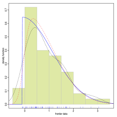
The left panel of Figure 1 displays these data together with their histogram and two fitted curves: one corresponds to the MLE, another one is a non-parametric kernel-type estimate, using a Gaussian kernel with bandwidth chosen by cross-validation, and the third curve will be described later on. Since $\hat{\alpha}=\infty$, the latter curve is a shifted and scaled $\chi$ distribution, with origin just below the smallest sample value. The right-side panel of this figure displays the deviance function

$$D(\alpha)=2\>\{\log L^{*}(\hat{\alpha})-\log L^{*}(\alpha)\}$$

where $L^{*}(\alpha)$ denotes the profile likelihood for $\alpha$. The curve, which appears to be monotonically decreasing, becomes flat for large $\alpha$.

Figure 1: Frontier data. Left panel: rug-plot and histogram with superimposed MLE fit (continuous line), non-parametric fit (dashed line) and MPLE fit (dot-dashed line). Right panel: deviance function of $\alpha$.

As mentioned earlier, the inclusion of the limiting points $\alpha=\pm\infty$ in the parameter space is admissible for distribution 1. However, $\alpha=\pm\infty$ represent a peculiar situation, not only because we are at the boundary of the parameter space, but in addition the support of the distribution collapses to the half-line, instead of the complete real line as for any finite $\alpha$.

When an unbounded estimate, $\hat{\alpha}=\pm\infty$, occurs there are two alternative aptitudes of a statistician. One is to say: if the MLE is $\hat{\alpha}=\infty$, we still take it; after all, this is an admissible value of the parameter. Notice however that, on the boundary on the parameter space, standard asymptotic distribution theory of MLE does not hold, and a special theory must be developed to obtain standard errors of the estimates. The other aptitude is to disregard $\hat{\alpha}=\infty$ as an anomaly of MLE. Not only this parameter point is peculiar for the general reasons indicated earlier, but in addition it often does not appear to actually describe the data in a satisfactory way. For instance, in the case of Figure 1, neither the histogram nor the non-parametric density estimate exhibit the extreme pattern in the data which are implied by the MLE value. Furthermore, as remarked by Azzalini & Capitanio, (1999), the sample index of skewness of the data, $0.902$, is well inside the admissible range of $\gamma_{1}$, about $\pm 0.99527$, whose extremal values correspond to $\alpha=\pm\infty$.

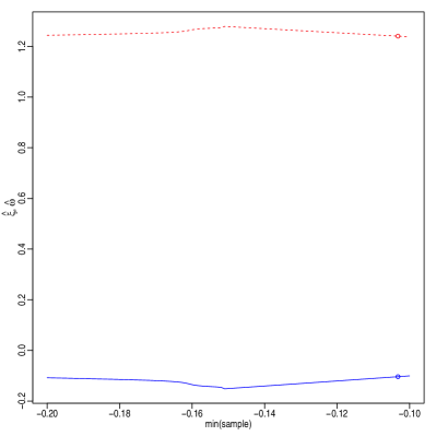
Yet another argument against the MLE choice is provided by the plots in Figure 2, which displays the behaviour of the three MLE components when the minimum sample value, $-0.1032$, is replaced by another value, $m$ say, which ranges from $-0.20$ to $-0.10$. While in the left panel $\hat{\xi}$ and $\hat{\omega}$ are very stable as $m$ moves along the range, the evolution of $\hat{\alpha}$ in the right panel has a dramatic discontinuity. When $m$ varies from $-0.2$ to $-0.152$, $\hat{\alpha}$ increases gradually from about $12$ to about $40$, but at $m=-0.151$ it jumps above $7200$. This value is however only where the numerical optimization procedure was stopped searching, but the search would lead to increasingly large values if it was left running, although the divergence of $\hat{\alpha}$ corresponds to a negligible increase of the log-likelihood function, as indicated by the right panel of Figure 1. Such a severe instability of an estimator in reaction to this minute variation of a single sample value is unacceptable on general grounds.

Figure 2: Frontier data: evolution of the MLE components when the minimum sample value ranges $-0.20$ to $-0.10$. The left panel refers to $\hat{\xi}$ (bottom curve) and $\hat{\omega}$ (top curve); the right panel refers to $\hat{\alpha}$. The bullets denote the estimates using the original sample minimum.

1.3 Alternative options

There appear to exist both general arguments and numerical evidence against the MLE solution, at least when it leads to boundary values of $\hat{\alpha}$. Notice that the problem cannot be cured by reparameterization, like for the singular information matrix, since any regular transformation maps boundary points of the parameter space $(\xi,\omega,\alpha)$ into boundary points of the new parameter space. In addition, if $\hat{\alpha}=\pm\infty$, the equivariance property of MLE would lead to take the transformed boundary point as the new MLE. Therefore a different estimation method need to be considered.

A number of alternative proposals have been put forward, adopting a range of different approaches. A preliminary solution to the problem has been put forward by Azzalini & Capitanio, (1999) in the discussion following the presentation of the frontier data. This is based on the consideration that the log-likelihood function varies little over a large span of the $\alpha$ axis; see the right panel of Figure 1 for a visual perception at leas of the profile version of the log-likelihood. It is then reasonable to take a value whose log-likelihood is below the maximum by a non-significant amount. While this technique works well in practice and it can applied also to a variety of similar problems, it leaves some arbitrary margin on the choice of the acceptable amount of drop from the maximum.

Sartori, (2006) has specialized the general bias-reduction method of Firth, (1993) to the present context. This technique replaces the usual likelihood equation $\ell^{\prime}(\alpha)=0$ by the modified form

$$\ell^{\prime}(\alpha)+M(\alpha)=0$$ (3)

and the correction term $M(\alpha)$ in the case $Z\sim\mathrm{SN}{}(0,1,\alpha)$ takes the form

$$M(\alpha)=-\frac{\alpha}{2}\>\frac{a_{4}(\alpha)}{a_{2}(\alpha)},\qquad a_{p}(\alpha)=\mathbb{E}\!\left\{\displaystyle{Z^{p}\>\zeta_{1}(\alpha\,Z)^{2}}\right\}$$ (4)

where $\zeta_{1}(x)=\zeta_{0}^{\prime}(x)$ is the inverse Mills ratio. Sartori shows that, for any sample, the modified likelihood equation has at least one finite solution. An interesting feature is the close similarity of the shape of $M(\alpha)$ with the derivative of the logarithm of Jeffreys’ uninformative prior. Since the three-parameter case $\mathrm{SN}{}(\xi,\omega^{2},\alpha)$ is hard to tackle via the general Firth’s method, Sartori introduces a specifically constructed two-step scheme.

In a Bayesian framework, Liseo & Loperfido, (2006) adopt the Jeffreys prior for $\alpha$, which they prove to be a proper distribution over the real line. For the thee-parameter case, an expression of the reference-integrated likelihood is obtained, although this is difficult to use for $n$ not small. Follow-up work has been done by Bayes & Branco, (2007) whose development includes a closed-form approximation

$$M(\alpha)\approx-\frac{3\,\alpha}{2}\left(1+\frac{8\,\alpha^{2}}{\pi^{2}}\right)^{-1}\,.$$ (5)

which is based on replacing the normal distribution function entering in the expression of $a_{p}(\alpha)$ by a rescaled logistic distribution. The subsequent simulation study confirms the closeness of the Sartori-Firth estimate to the Jeffreys’ posterior mode.

An alternative route has been taken by Greco, (2011) using a minimum Hellinger distance criterion, which also leads to finite estimates of $\alpha$ for the case $\mathrm{SN}{}(0,1,\alpha)$. This approach works for the three-parameter case as well, without introducing special adaptation. However it involves the choice of a specific density estimate and of the connected smoothing parameter, which influences the final outcome.

The above-recalled constructions lead to elegant results for the basic case $\mathrm{SN}{}(0,1,\alpha)$, but the three-parameter case $\mathrm{SN}{}(\xi,\omega^{2},\alpha)$ already poses non-trivial additional difficulties for the first two of them. The multivariate case has not been tackled at all, as far as we know, except for a very brief mention of Greco, (2011). The analogous problem with the skew-normal distribution replaced by the skew-$t$ distribution is inevitably more complex, because of one additional parameter involved and the diminished mathematical tractability; we shall review the existing results for the univariate case in Section 3.

The aim of the rest of the paper is to develop a procedure which can be applied to a range of situations, including the multivariate case, with the requirement that its behaviour is largely the same of the MLE, with only a minor modification to prevent boundary estimates. We first develop our proposal for the skew-normal distribution, and later extend it to the skew-$t$ distribution.

2 Penalization of the log-likelihood function

2.1 General remarks

Penalization of the log-likelihood function is a device which has been adopted in a number of problems to correct some undesirable behaviour of the regular MLE. Sartori, (2006, p. 4262) has remarked that 3 can be viewed in this light.

Our aim is to avoid divergent estimates of $\alpha$, in a formulation applicable to a wide range of situations of the context described earlier. To this end, consider a function of the form

$$\ell_{p}(\theta)=\ell(\theta)-Q$$ (6)

where $\ell(\theta)$ denotes the log-likelihood function for $\theta$ which denotes the whole set of parameters associated to the chosen parametric family, and $Q$ represents a non-negative quantity which penalizes the divergence of $\alpha$ and it remains $O_{p}(1)$ as $n$ increases. A value $\tilde{\theta}$ which maximizes $\ell_{p}(\theta)$ will be called a Maximum Penalized Likelihood Estimate (MPLE).

The log-likelihood functions which we have in mind are primarily of skew-normal type, and related ones discussed in Section 3, but part of the development can potentially be of interest also in other settings. It is assumed that $\ell(\theta)$ satisfies the standard conditions for consistency and asymptotic normality of the regular MLE, $\hat{\theta}$, as set for instance in Theorem 5.2.2 of Sen & Singer, (1993).

Besides the univariate distributions $\mathrm{SN}{}(0,1,\alpha)$ and $\mathrm{SN}{}(\xi,\omega^{2},\alpha)$, we consider also the multivariate skew-normal distribution $\mathrm{SN}{}_{d}(\xi,\Omega,\alpha)$ whose density function is

$$2\>\phi_{d}(x-\xi;\Omega)\>\Phi\left(\alpha^{\top}\omega^{-1}(x-\xi)\right),\qquad x\in\mathbb{R}^{d}\,,$$ (7)

where $\phi_{d}(x;\Omega)$ denotes the $\mathrm{N}{}_{d}(0,\Omega)$ density function and $\omega$ is a diagonal matrix formed by the standard deviations of $\Omega$; in this case $\alpha$ and $\xi$ are $d$-dimensional parameters. For these three parametric families, the parameter $\theta$ in 6 has $1$ or $3$ or $d(d+5)/2$ components, respectively.

The translation into mathematical notation of the above-indicated requirements for $Q$ is that

$$Q\geq 0\,,\qquad Q\big{|}_{\alpha=0}=0\,,\qquad\lim_{\alpha_{j}\to\pm\infty}Q=\infty$$ (8)

where $\alpha_{j}$ is the $j$-th component of $\alpha$, for $j=1,\dots,d$. For the SN distribution, and the ST distribution to be discussed later, $\log\,L$ does not diverge to $+\infty$ even when the MLE of $\alpha$ diverges; combining this fact with the third requirement in 8 we are ensured that 6 has a finite maximum in the interior of the parameter space. In a different context where some components of the MLE can diverge but the log-likelihood itself is bounded from above, the same argument applies provided the third condition in 8 is suitably adapted to the different parameter set.

In the next sections $Q$ will be a function of the parameters only, not depending on the data. This condition could be removed as long as $Q$ is $O_{p}(1)$; however, the mathematical treatment would be more elaborate and for simplicity we do not consider this case in detail. For the subsequent development we also require that $Q$ is twice differentiable with respect to $\theta$, and that $Q^{\prime\prime}(\theta)$ is a uniformly continuous mapping in a neighbourhood of the true parameter point. An additional sensible requirement, although not necessary for our construction, is that $Q$ increases monotonically with each $|\alpha_{j}|$.

Besides existence of $\tilde{\theta}$, another implication of this formulation concerns the first-order asymptotic distribution of $\tilde{\theta}$ when a random sample of size $n$ is available: as $n\to\infty$, this asymptotic distribution coincides with the one $\hat{\theta}$. This fact is intuitive on noticing that both $\ell(\theta)$ and $\ell_{p}(\theta)$ are $O_{p}(n)$ and they differ by $Q$, which is $O_{p}(1)$, but it can also easily be proved formally, under the above regularity conditions, following essentially an argument similar to Theorem 5.2.2 of Sen & Singer, (1993). We then conclude that $\tilde{\theta}$ is consistent with asymptotic distribution

$$\sqrt{n}(\tilde{\theta}-\theta)\hbox{$\leavevmode\nobreak\ \stackrel{{\scriptstyle d}}{{\longrightarrow}}\leavevmode\nobreak\ $}\mathrm{N}{}\left(0,i_{E}(\theta)^{-1}\right),\quad\mathrm{when\leavevmode\nobreak\ }n\to\infty\,,$$ (9)

where $i_{E}(\theta)$ denotes the expected Fisher information for a single observation. A more informative expression can be obtained by expanding $\ell^{\prime}_{p}(\tilde{\theta})$ from the point $\hat{\theta}$ as follows:

$$0 = \ell^{\prime}_{p}(\tilde{\theta})$$

$$= \ell_{p}^{\prime}(\hat{\theta})+\ell_{p}^{\prime\prime}(\hat{\theta})\,(\tilde{\theta}-\hat{\theta})+o(\|\tilde{\theta}-\hat{\theta}\|)$$

$$= -Q^{\prime}(\hat{\theta})+\ell_{p}^{\prime\prime}(\hat{\theta})\,(\tilde{\theta}-\hat{\theta})+o(\|\tilde{\theta}-\hat{\theta}\|)$$

where $\ell^{\prime\prime}_{p}$ denotes the matrix of second order derivatives of $\ell_{p}$. We can then write

$$\tilde{\theta}-\hat{\theta}=\ell_{p}^{\prime\prime}(\hat{\theta})^{-1}Q^{\prime}(\hat{\theta})+R$$ (10)

where the remainder $R$ is of smaller order in probability than the leading term under the assumption of uniform local continuity of $Q^{\prime\prime}$. Therefore $\tilde{\theta}$ and $\hat{\theta}$ differ by $O_{p}(n^{-1})$.

It is common practice to obtain standard errors for $\hat{\theta}$ via an approximation of its covariance matrix with the inverse of the observed information matrix $-\ell^{\prime\prime}(\hat{\theta})^{-1}=I_{O}(\hat{\theta})^{-1}$, say. Combining the fact $\tilde{\theta}-\hat{\theta}=O_{p}(n^{-1})$ with local continuity of $Q^{\prime\prime}(\theta)$, we obtain the matching approximation

$$\textrm{var}\!\left\{\displaystyle{\tilde{\theta}}\right\}\approx-\ell^{\prime\prime}_{p}(\tilde{\theta})^{-1}\,.$$ (11)

2.2 On the choice of $Q$

The above formulation leaves an extremely wide set of options as for choice of the penalty function. One way for selecting $Q$, or nearly equivalently for selecting $M(\theta)=-Q^{\prime}(\theta)$, is to require that the first order term of the bias is eliminated. This is the route taken Firth, (1993) where the requirement of bias reduction is adopted at the onset of the construction; see also further work by Kosmidis & Firth, (2009). If we insert $\pm\theta$ on the left-hand side of 10 and compute expected values, then the leading terms are

$$\mathrm{bias}(\tilde{\theta})\approx\mathrm{bias}(\hat{\theta})+I_{E}(\theta)^{-1}\>\mathbb{E}\!\left\{\displaystyle{M(\theta)}\right\}$$

where $I_{E}(\theta)=n\,i_{E}(\theta)$ is the expected information matrix and of course computation of the expected value of $M(\theta)$ is void when $Q$ does not depend on the data. On equating the left side of this expression to $0$, we obtain the condition

$$\mathbb{E}\!\left\{\displaystyle{M(\theta)}\right\}=-I_{E}(\theta)\,\mathrm{bias}(\hat{\theta})$$

which must be completed by substitution of $\mathrm{bias}(\hat{\theta})$ with the first-order term of the MLE bias, given by Cox & Snell, (1968). When $M(\theta)$ does not depend on the data, we arrive at an estimating equation of type 3.

One difficulty with the bias reduction criterion for selecting $M$ is the technical difficulty of working out the explicit expression of $\mathrm{bias}(\hat{\theta})$. In the skew-normal case, only the one-parameter case leads to the relatively simple form 4, where however the coefficients $a_{p}(\alpha)$ do not have an explicit expression.

Moreover, as reminded by Kosmidis & Firth, (2009), “Point estimation and unbiasedness are, of course, not strong statistical principles. The notion of bias, in particular, relates to a specific parameterization of a model: for example, the unbiasedness of the familiar sample variance $S^{2}$ as an estimator of $\sigma^{2}$ does not deliver an unbiased estimator of $\sigma$ itself”. We agree with this view, and in the development to follow the requirement of unbiasedness will be taken into account but not in a prescriptive form.

We conclude this section with a qualitatively motivated choice for $Q$ in the case of a multivariate skew-normal distribution. It has repeatedly emerged that many salient features of the family 7 depend on the parameters via only the scalar quantity

$$\alpha_{*}^{2}=\alpha^{\top}\bar{\Omega}\alpha$$

where $\bar{\Omega}=\omega^{-1}\,\Omega\,\omega^{-1}$ is the correlation matrix associated to $\Omega$. The prominent role of $\alpha_{*}^{2}$ appears in a number of results of Azzalini & Capitanio, (1999) and of Arellano-Valle & Azzalini, (2008); in the latter paper the dependence is expressed indirectly via the monotonically related quantity $\beta_{0}^{2}=2\,\alpha_{*}^{2}/\{\pi+(\pi-2)\alpha_{*}^{2}\}$.

It is then natural to introduce a function $Q$ in 6 which depends on $\theta$ only via $\alpha_{*}^{2}$. Combining this choice with the requirements 8 and the consideration that a logarithmic form of dependence would keep the modification of the original log-likelihood to a minimum also for diverging $\alpha_{*}$, we arrive at the formulation

$$Q=c_{1}\,\log(1+c_{2}\,\alpha_{*}^{2})$$ (12)

where $c_{1}$ and $c_{2}$ are positive constants. This is not yet a fully specified penalty function, but the set on alternative options is now greatly reduced.

2.3 On the choice of $Q$ in the skew-normal case

We focus initially on the scalar skew-normal distribution. In this case $Q$ and its first derivative take the form

$$Q(\alpha)=c_{1}\,\log(1+c_{2}\alpha^{2})\,,\qquad Q^{\prime}(\alpha)=2\,c_{1}\,c_{2}\frac{\alpha}{1+c_{2}\alpha^{2}}\,.$$ (13)

Note that approximation 5 of $M(\alpha)$ is of type $-Q^{\prime}(\alpha)$ with $c_{1}=3\,\pi^{2}/32$, $c_{2}=8/\pi^{2}$, but the intended use of $Q(\alpha)$ is not only for the one-parameter case to which 5 applies.

We want to develop an alternative approximation to $M(\alpha)$ defined by 4. The reason for this search is partly to obtain an approximation with stronger theoretical support and, more importantly, to explore a direction which can extended to the skew-$t$ case which will be considered later.

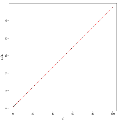
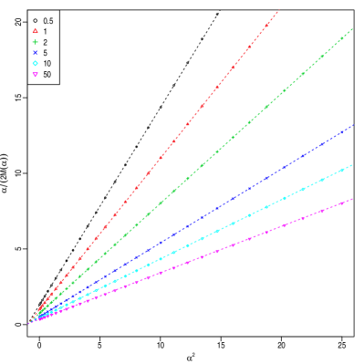
First, note that $a_{2}(\alpha)$ and $a_{4}(\alpha)$ are even functions of $\alpha$. This fact has been proved for $a_{2}(\alpha)$ by Liseo & Loperfido, (2006) but the proof extends immediately to any $a_{p}(\alpha)$ with even $p$. Hence $a_{2}/a_{4}$ depends on $\alpha$ only via $\alpha^{2}$. Next we observe that the numerical behaviour of $a_{2}/a_{4}$ is remarkably linear with respect to $\alpha^{2}$ as shown by the left panel of Figure 3 which displays the value of $a_{2}/a_{4}$ at 31 equally spaced points of $\alpha$ between 0 and 10; the interpolating line will be described shortly.

Figure 3: Left panel: values of $a_{2}(\alpha)/a_{4}(\alpha)$ for SN distributions, numerically evaluated at a grid of points, plotted versus $\alpha^{2}$ and superimposed approximating line. Right panel: $Q$ function obtained by numerical integration of $-M(\alpha)$ (continuous line), by integration of its approximation 5 (dashed line) and by $Q$ described in the text (dot-dashed line)

Therefore we approximate $a_{2}/a_{4}$ by a function of the form $e_{1}+e_{2}\alpha^{2}$ and we select $e_{1}$ and $e_{2}$ by matching $a_{2}/a_{4}$ and $e_{1}+e_{2}\alpha^{2}$ at $\alpha^{2}=0$ and $\alpha^{2}\to\infty$. To this end, re-write $a_{p}(\alpha)$ as

$$a_{p}(\alpha)=\sqrt{\frac{2}{\pi}}\>\frac{1}{(1+\alpha^{2})^{p+1/2}}\>\mathbb{E}\!\left\{\displaystyle{X^{p}\,\zeta_{1}(\delta\,X)}\right\}$$

where $X\sim\mathrm{N}{}(0,1)$ and $\delta=\delta(\alpha)=\alpha/\sqrt{1+\alpha^{2}}$. Hence

$$\frac{a_{2}(\alpha)}{a_{4}(\alpha)}=(1+\alpha^{2})\frac{\mathbb{E}\!\left\{\displaystyle{X^{2}\,\zeta_{1}(\delta\,X)}\right\}}{\mathbb{E}\!\left\{\displaystyle{X^{4}\,\zeta_{1}(\delta\,X)}\right\}}\approx e_{1}+e_{2}\,\alpha^{2}$$

leading to

$$e_{1} = \frac{a_{2}(0)}{a_{4}(0)}=\frac{\mathbb{E}\!\left\{\displaystyle{X^{2}}\right\}}{\mathbb{E}\!\left\{\displaystyle{X^{4}}\right\}}=\frac{1}{3}\,,$$

$$e_{2} = \lim_{\alpha^{2}\to\infty}\left\{\frac{1+\alpha^{2}}{\alpha^{2}}\,\frac{\mathbb{E}\!\left\{\displaystyle{X^{2}\,\zeta_{1}(\delta\,X)}\right\}}{\mathbb{E}\!\left\{\displaystyle{X^{4}\,\zeta_{1}(\delta\,X)}\right\}}-\frac{e_{1}}{\alpha^{2}}\right\}=\frac{\mathbb{E}\!\left\{\displaystyle{X^{2}\,\zeta_{1}(X)}\right\}}{\mathbb{E}\!\left\{\displaystyle{X^{4}\,\zeta_{1}(X)}\right\}}\approx 0.2854166$$ (14)

where the final coefficient was obtained by numerical integration. The line plotted in the left panel of Figure 3 has intercept $e_{1}$ and slope $e_{2}$.

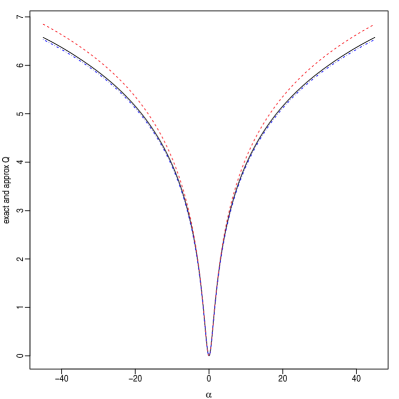
The right panel of Figure 3 displays three curves: the continuous line is the curve obtained by numerical integration of $-M(\alpha)$ defined by 4, and it coincides up to the change of sign with the continuous curve in Figure 1(b) of Sartori, (2006); the dashed line is the $Q$ function in 13 with $c_{1}=3\,\pi^{2}/32$, $c_{2}=8/\pi^{2}$, corresponding to the integral of approximation 5; the dot-dashed line is the curve $Q$ with coefficients

$$c_{1}=1/(4\,e_{2})\approx 0.875913,\qquad c_{2}=e_{2}/e_{1}\approx 0.856250\,,$$ (15)

whose graph is barely distinguishable from the essentially exact continuous curve.

This choice of $Q$ with coefficients 15 is motivated by the Sartori-Firth formulation for the case $\mathrm{SN}{}(0,1,\alpha)$. However, we adopt the same penalty function more generally, to the three-parameter case $\mathrm{SN}{}(\xi,\omega^{2},\alpha)$, since the motivation for introducing a penalization of the log-likelihood function came solely from its behaviour with respect to $\alpha$. When this procedure is applied to the frontier data, the estimates of $(\xi,\omega,\alpha)$ are $(-0.034,1.165,6.256)$, quite close to the true parameters $(0,1,5)$ and also close to the Sartori values $(-0.106,1.234,6.243)$, whose first two components coincide with the MLE. The graphical outcome of the MPLE is represented by the dot-dashed curve in the left panel of Figure 1. It is also worth mentioning that a shape parameter $\alpha=6.256$ corresponds to an index of skewness $\gamma_{1}=0.899$, very close to the sample index of skewness, $0.902$.

Consider now a $d$-dimensional skew-normal distribution 7, initially in the case of a location- and scale-free variable $Z\sim\mathrm{SN}{}_{d}(0,\bar{\Omega},\alpha)$ where $\bar{\Omega}$ is a correlation matrix. Recall the canonical transformation $Z^{*}=A^{*}\,Z$ introduced in Proposition 4 of Azzalini & Capitanio, (1999), such that $Z^{*}$ has $d$ independent components of which one (the first one, say) has distribution

$$\mathrm{SN}{}(0,1,\alpha_{*}),\qquad\alpha_{*}=\left(\alpha^{\top}\bar{\Omega}\alpha\right)^{1/2}\,,$$

and the other $d-1$ components are $\mathrm{N}{}(0,1)$. More specifically, an explicit expression of the transformation, given in the proof available in the full version of the paper, is

$$Z^{*}=(C^{-1}P)^{\top}\>Z$$ (16)

where $C$ is such that

$$\bar{\Omega}=C\>C^{\top}$$

and $P$ is an orthogonal matrix whose first column is proportional to $C\alpha$. We can then write

$$Z^{*}\sim\mathrm{SN}{}_{d}(0,I_{d},\alpha_{Z^{*}}),\qquad\alpha_{Z^{*}}=(\alpha_{*},0,\dots,0)^{\top}\,.$$

Assume now that a random sample $z=(z_{1},\dots,z_{n})$ is drawn from $Z\sim\mathrm{SN}{}_{d}(0,\bar{\Omega},\alpha)$. To estimate its parameters, we can proceed as follows.

• The sample $z$ can be converted into an equivalent sample $z^{*}=(z_{1}^{*},\dots,z_{n}^{*})$ drawn from $Z^{*}\sim\mathrm{SN}{}_{d}(0,I_{d},\alpha_{Z^{*}})$ on setting

  $$z_{i}^{*}=(C^{-1}P)^{\top}\>z_{i}\qquad(i=1,\dots,n).$$

  The determinant of the Jacobian is $\det(C^{\top}\>P)=\det(C)=\det(\bar{\Omega})^{1/2}\,.$

• We now have a sample of size $n$ from $\mathrm{SN}{}(0,1,\alpha_{*})$ and $d-1$ samples of size $n$ from $\mathrm{N}{}(0,1)$. For the first sample, we adopt the above-described scheme, hence the log-likelihood function is as on 2 with $\alpha$ replaced by $\alpha_{*}$ and the penalty function is 12 with coefficients which can be taken as in 15.

• Now we can revert back the $z^{*}$ sample to the original $z$, for which we write the usual log-likelihood, except that in this process we have introduced the penalty factor for $\alpha$. In conclusion the penalized log-likelihood is

  $$\ell_{p}(\theta) = \ell(\theta)-c_{1}\,\log(1+c_{2}\alpha_{*}^{2})$$ (17)

  $$= \sum_{i=1}^{n}\left(\log\phi_{d}(z_{i};\bar{\Omega})+\zeta_{0}(\alpha^{\top}z_{i})\right)-c_{1}\,\log(1+c_{2}\alpha_{*}^{2})\,.$$

The following remarks apply. First, the transformations from $z$ to $z^{*}$ and then back to $z$ are conceptual steps which serve only as an argument to introduce the penalty factor, and support its present form, and they do not need to be actually performed. Second, note that, although $d$ does not appear explicitly in the penalty factor, it does have an effect since $\alpha_{*}^{2}$ reflects $d$ indirectly, via the increase of the number of summands in its expression. As a simple example, take the case where $\alpha$ is a vector with $d$ identical components $\alpha_{0}$ and $\bar{\Omega}=I_{d}$, then $\alpha_{*}^{2}=d\,\alpha_{0}^{2}$.

Now move to the general case of 7 and consider a random sample $y=(y_{1},\dots,y_{n})$ from $Y\sim\mathrm{SN}{}_{d}(\xi,\Omega,\alpha)$. By adapting the $\ell(\theta)$ term in 17 for the presence of location and scale parameters, we arrive at

$$\ell_{p}(\theta) = \sum_{i=1}^{n}\left[\log\phi_{d}(y_{i}-\xi_{i};\Omega)+\zeta_{0}(\alpha^{\top}\omega^{-1}(y_{i}-\xi_{i}))\right]-c_{1}\,\log(1+c_{2}\alpha_{*}^{2})$$ (18)

where $\theta^{\top}=(\xi^{\top},(\mathop{\mathrm{vech}}\nolimits\Omega)^{\top},\alpha^{\top})$; here $\mathop{\mathrm{vech}}\nolimits$ is the operator which stacks the lower triangle of a matrix in a vector.

2.4 LRT-type statistic and another estimate

Consider now the likelihood-ratio test (LRT) statistics in its standard version and the analogous one for the penalized log-likelihood 6, that is

$$W=W(\theta)=2\{\ell(\hat{\theta})-\ell(\theta)\},\qquad W_{p}=W_{p}(\theta)=2\{\ell_{p}(\tilde{\theta})-\ell_{p}(\theta)\}\,.$$

From the results of Section 2.1, we can say that the null distribution of $W_{p}$ is of $\chi^{2}$ type, similarly to $W$.

Both intuition and the results of Section 2.1 suggest that $W$ and $W_{p}$ must be strongly associated. Some numerical exploration confirms this idea but it also exhibits that the type of dependence is quite peculiar. This is illustrated in the left plot of Figure 4 which refers to a set of 5000 samples of size $n=1000$ from the distribution $\mathrm{SN}{}(0,1,\alpha)$ with $\alpha=3$; hence in this case $\theta$ is $\alpha$. To increase readability, the right plot of the same figure displays a subset of the earlier points over a reduced plotting area. The obvious feature of this figure is that the joint distribution of $(W,W_{p})$ is strongly concentrated along two branches. A closer inspection indicates that the top branch is made of points where both $\hat{\alpha}$ and $\tilde{\alpha}$ underestimate the true $\alpha=3$, the bottom branch is composed by points where both $\hat{\alpha}$ and $\tilde{\alpha}$ overestimate, and the darker points around in the bottom left corner are those where $\hat{\alpha}-\alpha$ and $\tilde{\alpha}-\alpha$ take opposite signs. Note that the points with opposite signs of the estimation error are whose with smaller values of both $W$ and $W_{p}$, hence those where the estimation error is smaller is size.

Figure 4: Scatter plot of simulated values of $W(\alpha)$ and $W_{p}(\alpha)$ for samples of size $n=100$ from $\mathrm{SN}{}(0,1,\alpha)$ when $\alpha=3$. Samples where both $\hat{\theta}$ and $\tilde{\theta}$ overestimate $\alpha$ are marked by grey diamonds, those where both underestimate are denoted by grey triangles, those with mixed signs are denoted by black circles. The right-side plot refers a subset of the sampled values and it shows the enlarged picture of a smaller area. The dashed line is the identity.

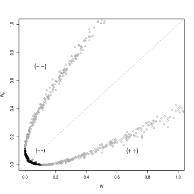
The pattern displayed in Figure 4 appears also in other simulation experiments. This behaviour, combined with the final remark of the previous paragraph, suggests an alternative estimate $\bar{\theta}$ defined as a solution of $W=W_{p}$, written more explicitly as

$$\bar{\theta}=\{\theta:W(\theta)-W_{p}(\theta)=0\}$$ (19)

or equivalently

$$\bar{\theta}=\{\theta:Q(\theta)=q(y)\},\qquad q(y)=\ell(\hat{\theta})-\ell(\tilde{\theta})+Q(\tilde{\theta})\,.$$ (20)

Note that $q(y)\geq 0$, with strict inequality if we exclude limiting cases. For the existence of this solution we need that (i) $W_{p}$ and $W$ are finite, and (ii) there exist points of the parameter space with opposite signs of $W_{p}-W$. In the context of skew-normal distribution, $\ell(\hat{\theta})$ and $\ell_{p}(\tilde{\theta})$ are bounded, so condition (i) holds. As for condition (ii), it holds because of the following facts:

$$W(\tilde{\theta})>0, W_{p}(\hat{\theta})>0,$$

$$W_{p}(\tilde{\theta})=0, W(\hat{\theta})=0,$$

$$W_{p}(\tilde{\theta})-W(\tilde{\theta})<0, W_{p}(\hat{\theta})-W(\hat{\theta})>0\,.$$ (21)

In the multiparameter case, 19 defines a surface in the parameter space, not a single point. In this case we complement 19 with the condition that $\bar{\theta}$ must lie on the segment joining $\hat{\theta}$ and $\tilde{\theta}$. Since inequalities 21 ensure that $\hat{\theta}$ and $\tilde{\theta}$ lie on opposite sides of the surface, this intersection point exists. From the computational viewpoint, $\bar{\theta}$ can be located efficiently, via a one-dimensional search along this segment, irrespectively of the dimension of $\theta$.

When $Q$ is chosen of the form 12, 20 takes a simple form, since the solution of $c_{1}\log(1+c_{2}\alpha_{*}^{2})=q(y)$ corresponds to the equation of an ellipsoid, that is $\alpha^{\top}\bar{\Omega}\alpha=r(y)$, where $r(y)=[e^{q(y)/c_{1}}-1]/c_{2}$.

2.5 Simulation study

The above estimation methods have been studied via numerical simulations. The first study has considered samples from $\mathrm{SN}{}(0,1,\alpha)$ where $\alpha$ was the only parameter to be estimated, and the true value was $\alpha=5$. For each generated sample, four estimators have been computed: classical MLE, MPLE with penalty 13 and coefficients 15, the Sartori–Firth estimator defined by 3-4, the estimator defined by the condition $W_{p}=W$ in 19. These estimates have been computer for $10^{6}$ replicated samples, for each of sample sizes $n=50,100,250,350,500,1000$.

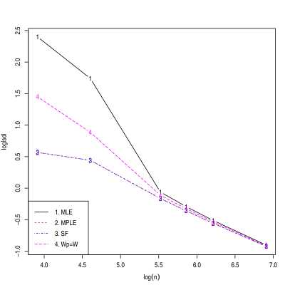
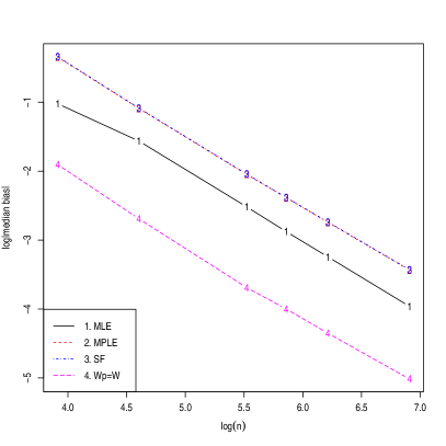
The final outcome is summarized graphically in the four panels of Figure 5, where the curves associated to the estimators are numbered $1$ to $4$. Four log-transformed summary quantities are plotted versus $\log n$; they are: absolute bias (top left), standard deviation (top right), absolute median bias (bottom left), inter-quartile range (bottom right). The cases where $\hat{\alpha}$ diverged have been excluded from the computation of these summaries, in agreement with Sartori, (2006) and Bayes & Branco, (2007).

Figure 5: Simulation study of the distributions of four estimators for samples of size $n=50,100,250,350,500,1000$ from $\mathrm{SN}{}(0,1,\alpha)$ when $\alpha$ only is estimated and the true value is $\alpha=5$; for each sample size $10^{6}$ replicates have been generated. The four estimators are 1:MLE, 2:MPLE, 3:SF, 4:$W_{p}=W$, but on three of the four panels MPLE and SF are graphically coincident. Top left panel: $\log|\mathrm{bias}|$, top right: log standard deviation, bottom left: $\log|\mathrm{median\leavevmode\nobreak\ bias}|$, bottom right: log IQR; in all case the horizontal axis represents $\log n$.

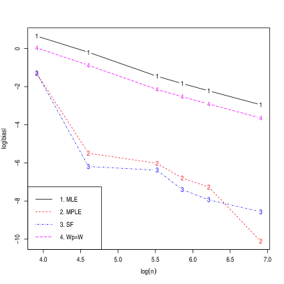
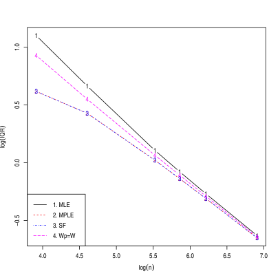
The doubly logarithmic scale has been adopted for simplifying interpretation of the curves. This is especially so for the top left panel, since the bias is expected to decrease at rate $n^{-1}$ for the MLE, and at rate $n^{-2}$ for the Sartori-Firth method and its close approximation MPLE. We do in fact observe that the slopes of these curves are close to $-1$ and $-2$ respectively. The top left panel confirms the theoretical expectations, displaying a clear improvement of SF and MPLE over MLE; the estimator 19 has a bias somewhat lower than MLE but decreasing at the same rate. MPLE and SF are very similar to each other, with only some discrepancy at the right end, with $n=1000$, where the bias is very small indeed and the numerical approximation involved in evaluating the coefficients $a_{p}(\alpha)$ in 4 may have perturbed slightly the exact implementation of the SF method.

The message emerging from the bottom left panel, which plots the logarithm of the median bias, is radically different. Estimator 19 is markedly preferable to the others, MLE is second best, and the other two are equivalent up to the point that their curves are superimposed. For all the curves the slope is near to $-1$, which means ad the rate of decrease $n^{-1}$ for the median bias, and the differences are only in the intercepts. Median unbiasedness is not often considered in theoretical work, presumably because it is a more difficult aspect to evaluate compared to mean unbiasedness; it has however the important advantage over mean unbiasedness that it is preserved under monotone parameter transformation.

The two right-side panels convey very similar messages as for variability of the four contenders: SF and MPLE have the smallest variability, both on the scale of standard deviation and of the inter-quartile range, and they are essentially equivalent to each other with superimposed curves; MLE has the largest variability and estimator 19 sits in between the others. Differently from the left-side plots, however, here the differences vanish as $n$ diverges, and they are effectively almost negligible from $n=250$ onwards.

The usual combination of bias and variance is given by the mean square error, or by its square root. If the logarithm of either of them is plotted versus $\log n$, the graphical appearance is virtually identical to the top right panel of Figure 5. If comparisons are based on moment-based quantities, the overall indications are then that (i) MPLE and SF are preferable to the others, at least for small and moderate $n$, (ii) MPLE and SF are effectively equivalent. It is less clear how to combine the two bottom panels into a single summary plot, but we note that also here the vertical scale of right-side panel has a larger order of magnitude than the left-side panel; hence its behaviour would dominate in any reasonable combination of the two.

In a second set of simulations, the data have still been sampled from a skew-normal distribution but now all three parameters are regarded as unknown, so that the reference set of distributions is of type $\mathrm{SN}{}(\xi,\omega^{2},\alpha)$. To ease comparisons, the parameter values and the sample sizes have been taken to be the same of Table 2 of Sartori, (2006), that is $\xi=0$, $\omega=1$, $\alpha=5,10$, with sample sizes $n=50,100,200$, but here a substantially larger number of replicates has been generated for each sample size, namely $10^{5}$. In all cases the location and scale parameters were $\xi=0$ and $\omega=1$. Table 1 reports the summary values for three estimators, that is MLE, MPLE and 19; for the last one, only the estimate of $\alpha$ is given, since the first two components of the estimate coincide with those of MPLE.

Inspection of the Table 1 confirms the improvement of $\tilde{\alpha}$ over $\hat{\alpha}$ and its overall similarity of the bias of $\tilde{\alpha}$ with the analogous entry in Table 2 of Sartori, (2006). Notice that, $\hat{\alpha}$ and $\tilde{\alpha}$ are now no longer essentially coincident as they were in the one-parameter case. In interpreting the bias and standard deviation of $\hat{\alpha}$ one must bear in mind that this have been computed excluding the case with diverging estimates; in practical term, we have taken $|\hat{\alpha}|>100$ as an indication of a diverging estimate. The exclusion of the diverging estimates has a relevant effect especially in the present setting where the probability of this event appears to be appreciably higher than in the one-parameter case; for instance with $n=50$ and $\alpha=5$ this probability is now about $0.139$, while it is only $0.039$ in the one-parameter case examined earlier. Bias and variability of $\tilde{\xi}$ and $\tilde{\omega}$ are somewhat higher than those of the MLE’s, $\hat{\xi}$ and $\hat{\omega}$, at least for $n=50$ and to some extent for $n=100$. It is then conceivable to adopt $\hat{\xi}$ and $\hat{\omega}$ as estimates of location and scale, and $\tilde{\alpha}$ for estimating shape, similarly to the strategy of Sartori. This choice is advantageous as for formal properties, but it has the logical drawback of the lack of a unique estimation criterion. Also in this setting, the estimate $\bar{\alpha}$ has low median bias, but this is paid by a substantial increase in variability.

Table 1: Summary quantities of the distribution of MLE, MPLE and 19 estimating the parameters $(\xi,\omega,\alpha)$ of a distribution $\mathrm{SN}{}(0,1,\alpha)$ when $\alpha=5,10$, based on a sample of size $n=50,100,200$. All entries are based on $10^{5}$ replicated samples.

$\alpha$	$n$		$\hat{\xi}$	$\hat{\omega}$	$\hat{\alpha}$	$\tilde{\xi}$	$\tilde{\omega}$	$\tilde{\alpha}$	$\bar{\alpha}$
5	50	mean bias	$0.0235$	$-0.0209$	$1.472$	$0.1740$	$-0.1252$	$-1.411$	$1.808$
		median bias	$0.0028$	$-0.0160$	$0.124$	$0.0884$	$-0.1023$	$-1.726$	$-0.610$
		std. dev.	$0.1502$	$0.1411$	$4.974$	$0.2661$	$0.1677$	$2.600$	$7.641$
		$\mathbb{P}\!\left\{\displaystyle{\hat{\alpha}=\infty}\right\}$			$0.139$
	100	mean bias	$0.0060$	$-0.0075$	$1.442$	$0.0534$	$-0.0499$	$-0.456$	$0.866$
		median bias	$0.0002$	$-0.0066$	$0.263$	$0.0379$	$-0.0456$	$-0.872$	$-0.306$
		std. dev.	$0.0839$	$0.0959$	$4.896$	$0.1118$	$0.1011$	$2.320$	$5.615$
		$\mathbb{P}\!\left\{\displaystyle{\hat{\alpha}=\infty}\right\}$			$0.023$
	200	mean bias	$0.0029$	$-0.0036$	$0.592$	$0.0216$	$-0.0222$	$-0.195$	$0.197$
		median bias	$0.0005$	$-0.0035$	$0.150$	$0.0181$	$-0.0216$	$-0.410$	$-0.152$
		std. dev.	$0.0544$	$0.0656$	$2.508$	$0.0558$	$0.0655$	$1.540$	$2.254$
		$\mathbb{P}\!\left\{\displaystyle{\hat{\alpha}=\infty}\right\}$			$0.001$
10	50	mean bias	$0.0225$	$-0.0235$	$0.788$	$0.1249$	$-0.1049$	$-3.992$	$3.497$
		median bias	$0.0076$	$-0.0210$	$-1.001$	$0.0685$	$-0.0898$	$-4.586$	$-1.070$
		std. dev.	$0.0910$	$0.1213$	$6.874$	$0.2038$	$0.1461$	$3.769$	$11.775$
		$\mathbb{P}\!\left\{\displaystyle{\hat{\alpha}=\infty}\right\}$			$0.345$
	100	mean bias	$0.0047$	$-0.0069$	$3.274$	$0.0393$	$-0.0418$	$-1.462$	$3.591$
		median bias	$-0.0004$	$-0.0067$	$0.527$	$0.0299$	$-0.0404$	$-2.481$	$-0.638$
		std. dev.	$0.0560$	$0.0830$	$9.399$	$0.0677$	$0.0845$	$4.580$	$12.840$
		$\mathbb{P}\!\left\{\displaystyle{\hat{\alpha}=\infty}\right\}$			$0.129$
	200	mean bias	$0.0015$	$-0.0025$	$2.575$	$0.0170$	$-0.0190$	$-0.422$	$1.583$
		median bias	$-0.0026$	$-0.0026$	$0.563$	$0.0140$	$-0.0188$	$-1.275$	$-0.360$
		std. dev.	$0.0374$	$0.0581$	$8.072$	$0.0375$	$0.0574$	$4.160$	$8.738$
		$\mathbb{P}\!\left\{\displaystyle{\hat{\alpha}=\infty}\right\}$			$0.021$

3 Extension to the skew-$t$ distribution

A distribution closely related to the skew-normal is the skew-$t$ whose density in the scalar case is

$$\frac{2}{\omega}\,t\left(\frac{x-\xi}{\omega};\nu\right)\>T\left(\alpha\>\frac{x-\xi}{\omega}\>\sqrt{\frac{\nu+1}{\nu+Q_{x}}};\nu+1\right),\qquad x\in\mathbb{R},$$ (22)

where $t(\cdot;\nu)$ is the Student’s $t$ density with $\nu>0$ degrees of freedom, $T(\cdot;\nu+1)$ is the $t$ distribution function for $\nu+1$ degrees of freedom and $Q_{x}=\omega^{-2}(x-\xi)^{2}$; here $\nu$ is a positive value which can be non-integer. This distribution allows regulation of the tail thickness via the additional parameter $\nu$. If a continuous random variable $Y$ has density function 22, we write $Y\sim\mathrm{ST}{}(\xi,\omega^{2},\alpha,\nu)$.

Initial work for applying the method of Firth to the case of a skew-$t$ distribution has been done by Sartori, (2006), who has considered estimation of $\alpha$ when the other parameters are known. For the three-parameter case ($\xi,\omega,\alpha$) with known $\nu$, Sartori has proposed a two-step procedure, similarly to the skew-normal case. This direction has been explored further by Lagos Álvarez & Jiménez Gamero, (2012) who have shown that the corresponding estimating equation is of the same form $M(\alpha)=0$ as in 4, with $a_{2}$ and $a_{4}$ replaced by suitably modified expressions which depend on $\nu$ besides $\alpha$. Moreover, they prove that $M(\alpha)=0$ always admits a finite solution when $\nu>2$.

In the ST case, we proceed similarly to the SN case to obtain a close approximation of the $M(\alpha)$ function. The plot on the left panel of Figure 6 plays a similar role of the left plot in Figure 3, except that we now have a sequence of points for each chosen values of $\nu$, specifically $\nu=\mbox{$\textstyle\frac{1}{2}$},1,2,5,10,50$, with different plotting symbols for each value of $\nu$. Also in this case there is a striking alignment of the points referring to the same $\nu$, particularly so if we consider the wide range of $\nu$ values considered.

Figure 6: Left panel: values of $\alpha/[-2\,M(\alpha)]$ for ST distributions, for $\nu=\mbox{$\textstyle\frac{1}{2}$},1,2,5,10,50$, numerically evaluated at a grid of points, plotted versus $\alpha^{2}$ and superimposed approximating line for each selected $\nu$. Right panel: $Q$ function obtained by numerical integration of $-M(\alpha)$ (continuous lines), and by $Q$ described in the text (dot-dashed lines).

For any fixed value of $\nu$, we approximate $\alpha/[-2\,M(\alpha)]$ by a function of the form

$$\frac{\alpha}{-2\,M(\alpha)}\approx e_{1\nu}+e_{2\nu}\,\alpha^{2}$$

whose coefficients $e_{1\nu}$ and $e_{2\nu}$ are obtained by matching the behaviour of the two sides at $\alpha^{2}=0$ and $\alpha^{2}\to\infty$. After some algebraic work summarized in an appendix, we arrive at the expressions

$$\begin{array}[]{rcl}e_{1\nu}&=&\displaystyle{\frac{g_{\nu}}{3}}\,,\\ e_{2\nu}&=&g_{\nu}^{2}\>\displaystyle{\frac{\mathbb{E}\!\left\{\displaystyle{X_{1}^{2}\zeta_{1}(X_{1};\nu+1)}\right\}}{\mathbb{E}\!\left\{\displaystyle{X_{3}^{4}\,\zeta_{1}\left(X_{3}\sqrt{(\nu+1)/(\nu+3)};\nu+1\right)}\right\}}}\end{array}$$ (23)

where

$$g_{\nu}=\displaystyle{\frac{(\nu+2)\,(\nu+3)}{(\nu+1)^{2}}}\,,\qquad\zeta_{1}(x;\nu)=\frac{t(x;\nu)}{T(x;\nu)}\,.$$ (24)

and $X_{k}\sim t_{\nu+k}$. The two expected values involved by $e_{2\nu}$ must be evaluated numerically. The dashed lines in the left panel of Figure 6 have intercepts and slopes given by 23; it is apparent that the lines interpolate the points described earlier almost exactly.

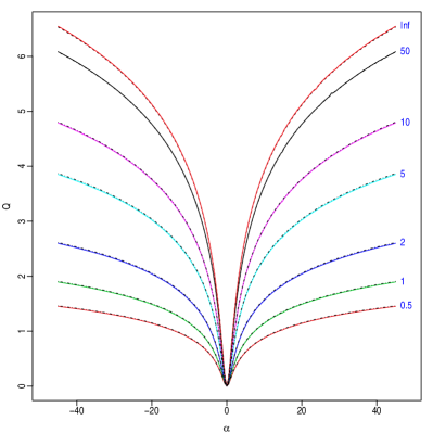
Again, the integral of $-M(\alpha)$ is then closely approximated by 13 with coefficients $c_{1}=1/(4\,e_{2\nu})$ and $c_{2}=e_{2\nu}/e_{1\nu}$. The right panel of Figure 6 displays the $Q$ function obtained by numerical integration of $-M(\alpha)$ as continuous lines, and their approximation of the form 13 as dot-dashed lines. The two set of lines are in fact virtually indistinguishable. Therefore this choice of $Q$ is essentially equivalent to the one of Sartori, (2006) and Lagos Álvarez & Jiménez Gamero, (2012) in the case $\mathrm{ST}{}(0,1,\alpha,\nu)$ when $\nu$ is regarded as known and only $\alpha$ is estimated, but it has the computational advantage of avoiding the numerical evaluation of a very large number of integrals, which are required when the numerical algorithm for solving $M(\alpha)=0$ searches over a range of $\alpha$ values.

At variance from the above-quoted authors, we adopt the penalty function just described also in the four parameter case $\mathrm{ST}{}(\xi,\omega^{2},\alpha,\nu)$, analogously to what we did for the three-parameter SN case. A point of practical concern in this process is that, when $\nu$ is not fixed, the algorithm for numerical optimization of $\ell_{p}(\theta)$ visits many candidate values of $\nu$, and each of them involves numerical evaluation of the two integrals involved by $e_{2\nu}$ in 23. To avoid these extensive integrations, we have explored a simple empirical approximation of $e_{2\nu}$.

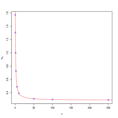
Some numerical exploration has show that $\log(e_{2\nu}/e_{2}-1)$ is very nearly a linear function of $\log(\nu+\gamma)$ where $\gamma=0.57721\dots$ is the Euler’s constant, and $e_{2}$ is the limiting value 14. This near linearity is visible in the left plot of Figure 7 which displays a set of numerically evaluated values $e_{2\nu}$, for a range of degrees of freedom from $\nu=0.25$ to $\nu=250$, transformed to $\log(e_{2\nu}/e_{2}-1)$ and plotted versus $\log(\nu+\gamma)$. The interpolating line fitted by least squares has intercept $1.37$ and slope $-1.00$ when rounded to two decimal places; these are the coefficients of the plotted line. In the right-side plot of the figure, the interpolation has been transformed back on the original scale, so that the continuous line superimposed to the points $(\nu,e_{2\nu})$ is the approximation

$$e_{2\nu}\approx e_{2}\left(1+\frac{4}{\nu+\gamma}\right)$$

which appears to work well. Clearly the other coefficient, $e_{1\nu}=g_{\nu}/3$, poses no problem.

Figure 7: Exact values of $e_{2\nu}$ and their approximating function on the transformed scale (left side plot) and on the original scale (right side plot).

In the multivariate case we proceed similarly to the skew-normal case, and consider a penalized log-likelihood function similar to 18, but the coefficients $c_{1}$ and $c_{2}$ now depend on $\nu$, and the summands of the first term are replaced by the logarithm of the multivariate skew-$t$ density function. This density is given by

$$2\,t_{d}(x-\xi;\Omega,\nu)\>T\left(\sqrt{\frac{d+\nu}{Q_{x}+\nu}}\,\alpha^{\top}\omega^{-1}(x-\xi);\,\nu+d\right),\qquad x\in\mathbb{R}^{d},$$ (25)

where $t_{d}(x;\Omega)$ denotes the $d$-dimensional Student’s $t$ density function with location $0$, scale matrix $\Omega$ and $\nu$ degrees of freedom; the earlier definition of $Q_{x}$ is now replaced by $Q_{x}=(x-\xi)^{\top}\Omega^{-1}(x-\xi)$.

4 Discussion

For the SN and ST distributions in the univariate and multivariate cases, we have examined a methodology which avoids the problem of estimates on the frontier of the parameter space which can occur with maximum likelihood estimation. The problem of estimates on the frontier is vanishing when the sample size diverges, but in practice, for small to moderate sample sizes, it arises with non-negligible probability and it has disturbing effects on the inferential process.

The present proposal is, in a way, closely connected with existing results, but there are differences. One is that the focus here is shifted from unbiasedness to the use of a penalty function $Q$ which can be chosen quite freely once a few requirements are satisfied. This is the basis of another difference from existing work: we have adopted the $Q$ function arising from the one-parameter cases, $\mathrm{SN}{}(0,1,\alpha)$ and $\mathrm{ST}{}(0,1,\alpha,\nu)$ with fixed $\nu$, as the starting point for the choice of $Q$ in more complex situations, that is multiparameter and multivariate settings.

There are various directions in which the present work can be extended, of which we mention a few.

• As it stands, the methodology presented here is applicable to the skew-normal and the skew-$t$ distributions, which are the two most commonly employed families from the broader set of skew-elliptical distributions. However the formulation could be adapted to other skew-elliptical families.

• The asymptotic results of Section 2.1 are all of first-order type. There is wide room for higher asymptotic theory; accuracy of approximation 11 is of special interest.

• Alternative choices of the penalty $Q$ could be considered provided the new function satisfies conditions 8 and those indicated shortly thereafter.

While these developments are interesting, the proposal at its present stage provides an already workable and quite general way to overcome what appears to us as the last obstacle to the systematic use of skew-normal and skew-$t$ distributions in routine statistical work.

Before closing, it is perhaps useful to point up that the adoption of the penalized likelihood formulation is compatible with the adoption of the centred parameterization mentioned in the introductory section as a tool to overcome the singularity of the information in the skew-normal case. The two mechanisms are conceptually distinct and they can coexist. Once the MPLE of the direct parameters have been obtained, they can be transformed into the centred parameter space, and the variance matrix of the MPLE estimates can be converted via the known Jacobian matrix of the transformation (Arellano-Valle & Azzalini,, 2008). For the skew-$t$ distribution the problem of singular information matrix at $\alpha=0$ does not arise for any $0<\nu<\infty$, as proved in Proposition 1 of Arellano-Valle, (2010).

Acknowledgement

This work was initiated while the first author was visiting the Departamento de Estadística, Pontificia Universidad Católica de Chile, whose generous hospitality is gratefully acknowledged. The research work of the second author was partially supported by grant FONDECYT 1085241, Chile

Appendix: Limiting behaviour of $M(\alpha)$ in the ST case

Consider a random variable $Z\sim\mathrm{ST}{}(0,1,\alpha,\nu)$ and its transformation $W=v(Z)\,Z$ where

$$v(z)=\sqrt{\frac{\nu+1}{\nu+z^{2}}}\,.$$

From Sartori, (2006), we write

$$l^{\prime}(\alpha) = \zeta_{1}(\alpha W;\nu+1)\,W,$$

$$l^{\prime\prime}(\alpha) = -\frac{\nu+1}{\nu+2}\left(1+\frac{\alpha^{2}W^{2}}{\nu+1}\right)^{-1}\zeta_{1}(\alpha W;\nu+1)\,W^{3}-\zeta_{1}(\alpha W;\nu+1)^{2}\,W^{2},$$

$$l^{\prime}(\alpha)^{3}+l^{\prime}(\alpha)\,l^{\prime\prime}(\alpha) = -\frac{\nu+1}{\nu+2}\left(1+\frac{\alpha^{2}W^{2}}{\nu+1}\right)^{-1}\alpha\,\zeta_{1}(\alpha W;\nu+1)^{2}\,W^{4}.$$

where $\zeta_{1}(x;\nu)$ is the function defined by 24. Let now $X_{k}\sim t(0,1;\nu+k)$, and define the random variables

$$V_{k\delta}=\sqrt{\frac{\nu+1}{\nu+k+(1-\delta^{2})\,X_{k}^{2}}}.$$

After some simple algebraic manipulations, where we use the relation

$$t(z;\nu)t\left(\alpha z\sqrt{\frac{\nu+1}{\nu+z^{2}}};\nu+1\right) = t(0;\nu)\sqrt{\frac{\nu+1}{\nu}}\,\left(\frac{\nu+1}{\nu+z^{2}}\right)^{-1/2}t\left(\sqrt{\frac{\nu+1}{\nu}}\,\sqrt{1+\alpha^{2}}\,z;\nu+1\right),$$

we obtain

$$\mathbb{E}\!\left\{\displaystyle{l^{\prime\prime}(\alpha)}\right\} = -\mathbb{E}\!\left\{\displaystyle{\zeta_{1}(\alpha W;\nu+1)^{2}\,W^{2}}\right\}$$

$$= -(1+\alpha^{2})^{-3/2}b_{\nu}\sqrt{\frac{\nu+1}{\nu}}\,\mathbb{E}\!\left\{\displaystyle{X_{1}^{2}\,V_{1\delta}\zeta_{1}(\delta X_{1}\,V_{1\delta};\nu+1)}\right\},$$

$$\mathbb{E}\!\left\{\displaystyle{l^{\prime}(\alpha)^{3}}\right\}+\mathbb{E}\!\left\{\displaystyle{l^{\prime}(\alpha)\,l^{\prime\prime}(\alpha)}\right\} = -\alpha\left(\frac{\nu+1}{\nu+2}\right)\mathbb{E}\!\left\{\displaystyle{\zeta_{1}(\alpha W;\nu+1)^{2}\left(1+\frac{\alpha^{2}W^{2}}{\nu+1}\right)^{-1}\,W^{4}}\right\}$$

$$= -\alpha(1+\alpha^{2})^{-5/2}b_{\nu}\sqrt{\frac{\nu}{\nu+3}}\left(\frac{\nu+1}{\nu+2}\right)^{2}\left(\frac{\nu+1}{\nu+3}\right)\>\times$$

$$\qquad\mathbb{E}\!\left\{\displaystyle{X_{3}^{4}\,V_{3\delta}\,\zeta_{1}(\delta X_{3}\,V_{3\delta};\nu+1)}\right\}$$

where $b_{\nu}=2t(0;\nu)$. Thus, using the Sartori–Firth formulae for $M(\alpha)$, we write

$$M(\alpha) = \frac{\mathbb{E}\!\left\{\displaystyle{l^{\prime}(\alpha)^{3}}\right\}+\mathbb{E}\!\left\{\displaystyle{l^{\prime}(\alpha)\,l^{\prime\prime}(\alpha)}\right\}}{-2\mathbb{E}\!\left\{\displaystyle{l^{\prime\prime}(\alpha)}\right\}}$$

$$= -\frac{\alpha}{2}\,\frac{\left(\frac{\nu+1}{\nu+2}\right){\small\mathbb{E}\!\left\{\displaystyle{\zeta_{1}(\alpha W;\nu+1)^{2}\left(1+\frac{\alpha^{2}\,W^{2}}{\nu+1}\right)^{-1}W^{4}}\right\}}}{\mathbb{E}\!\left\{\displaystyle{\zeta_{1}(\alpha W;\nu+1)^{2}\,W^{2}}\right\}}$$

$$= -\frac{\alpha(1+\alpha^{2})^{-5/2}b_{\nu}\sqrt{\frac{\nu}{\nu+3}}\left(\frac{\nu+1}{\nu+2}\right)^{2}\left(\frac{\nu+1}{\nu+3}\right)\,\mathbb{E}\!\left\{\displaystyle{X_{3}^{4}\,V_{3\delta}\,\zeta_{1}(\delta X_{3}\,V_{3\delta};\nu+1)}\right\}}{2(1+\alpha^{2})^{-3/2}b_{\nu}\sqrt{\frac{\nu}{\nu+1}}\,\mathbb{E}\!\left\{\displaystyle{X_{1}^{2}\,V_{1\delta}\,\zeta_{1}(\delta X_{1}\,V_{1\delta};\nu+1)}\right\}}.$$

Note that the second expression agrees with a matching one of Lagos Álvarez & Jiménez Gamero, (2012). From the last expression, we obtain

$$-\frac{\alpha}{2\,M(\alpha)} = (1+\alpha^{2})\left(\frac{\nu+2}{\nu+1}\right)^{2}\left(\frac{\nu+3}{\nu+1}\right)^{3/2}\frac{\mathbb{E}\!\left\{\displaystyle{X_{1}^{2}\,V_{1\delta}\,\zeta_{1}\left(\delta X_{1}\,V_{3\delta};\nu+1\right)}\right\}}{\mathbb{E}\!\left\{\displaystyle{X_{3}^{4}\,V_{3\delta}\,\zeta_{1}\left(\delta X_{3}\,V_{3\delta};\nu+1\right)}\right\}}$$

$$\approx e_{1\nu}+e_{2\nu}\alpha^{2}.$$

Thus, by noting that for $\alpha^{2}=0$

$$\mathbb{E}\!\left\{\displaystyle{X_{k}^{2r}\,V_{k0}}\right\} = \frac{b_{\nu+k}}{b_{\nu+k+1}}\sqrt{\frac{\nu+1}{\nu+k}}\left(\frac{\nu+k}{\nu+k+1}\right)^{(2r+1)/2}\mathbb{E}\!\left\{\displaystyle{X_{k+1}^{2r}}\right\}$$

$$= \left(\frac{b_{\nu+k}}{b}\right)^{2}\sqrt{\frac{\nu+1}{\nu+k}}\left(\frac{\nu+k}{2}\right)^{r}\frac{\Gamma[(\nu+k+1-2r)/2]}{\Gamma[(\nu+k+1)/2]}\frac{(2r)!}{2^{r}r!},$$

we arrive at

$$e_{1\nu} = \left(\frac{\nu+2}{\nu+1}\right)^{2}\left(\frac{\nu+3}{\nu+1}\right)^{3/2}\frac{\mathbb{E}\!\left\{\displaystyle{X_{1}^{2}V_{10}}\right\}}{\mathbb{E}\!\left\{\displaystyle{X_{3}^{4}V_{30}}\right\}}$$

$$= \frac{1}{3}\left(\frac{b_{\nu+1}}{b_{\nu+3}}\right)^{2}\left(\frac{\nu+2}{\nu+1}\right)^{3},$$

while

$$e_{2\nu} = \lim_{\alpha^{2}\to\infty}\left\{\frac{1+\alpha^{2}}{\alpha^{2}}\left(\frac{\nu+2}{\nu+1}\right)^{2}\left(\frac{\nu+3}{\nu+1}\right)^{3/2}\,\frac{\mathbb{E}\!\left\{\displaystyle{X_{1}^{2}V_{1\delta}\zeta_{1}\left(\delta X_{1}V_{1\delta};\nu+1\right)}\right\}}{\mathbb{E}\!\left\{\displaystyle{X_{3}^{4}V_{3\delta}\zeta_{1}\left(\delta X_{3}V_{3\delta};\nu+1\right)}\right\}}-\frac{e_{1\nu}}{\alpha^{2}}\right\}$$

$$= \left(\frac{\nu+2}{\nu+1}\right)^{2}\left(\frac{\nu+3}{\nu+1}\right)^{2}\,\frac{\mathbb{E}\!\left\{\displaystyle{X_{1}^{2}\,\zeta_{1}(X_{1};\nu+1)}\right\}}{\mathbb{E}\!\left\{\displaystyle{X_{3}^{4}\,\zeta_{1}\left(\sqrt{\nu+1}\,X_{3}/\sqrt{\nu+3};\nu+1\right)}\right\}}.$$

References

- Arellano-Valle, (2010) Arellano-Valle, R. B. (2010). The information matrix of the multivariate skew- distribution. Metron, LXVIII, 371–386. Special issue on Skew-symmetric and flexible distributions.
- Arellano-Valle & Azzalini, (2008) Arellano-Valle, R. B. & Azzalini, A. (2008). The centred parametrization for the multivariate skew-normal distribution. J. Multivariate Anal., 99, 1362–1382. Corrigendum: vol. 100 (2009), p. 816.
- Azzalini, (1985) Azzalini, A. (1985). A class of distributions which includes the normal ones. Scand. J. Statist., 12, 171–178.
- Azzalini, (2005) Azzalini, A. (2005). The skew-normal distribution and related multivariate families (with discussion). Scand. J. Statist., 32, 159–188 (C/R 189–200).
- Azzalini, (2011) Azzalini, A. (2011). Skew-normal distribution. In M. Lovric (Ed.), International Encyclopedia of Statistical Sciences, volume 19 (pp. 1342–1344). New York: Springer.
- Azzalini & Capitanio, (1999) Azzalini, A. & Capitanio, A. (1999). Statistical applications of the multivariate skew normal distribution. J. R. Statist. Soc., ser. B, 61(3), 579–602. Full version of the paper at arXiv.org:0911.2093.
- Bayes & Branco, (2007) Bayes, C. L. & Branco, M. D. (2007). Bayesian inference for the skewness parameter of the scalar skew-normal distribution. REBRAPE: Brazilian Journal of Probability and Statistics, 21(2), 141–163.
- Cox & Snell, (1968) Cox, D. R. & Snell, E. J. (1968). A general definition of residuals. J. R. Statist. Soc., ser. B, 30(2), 248–275.
- Firth, (1993) Firth, D. (1993). Bias reduction of maximum likelihood estimates. Biometrika, 80, 27–38. Amendment: vol. 82, 667.
- Genton, (2004) Genton, M. G., Ed. (2004). Skew-elliptical Distributions and Their Applications: a Journey Beyond Normality. Boca Raton, FL, USA: Chapman & Hall/CRC.
- Greco, (2011) Greco, L. (2011). Minimum Hellinger distance based inference for scalar skew-normal and skew- distributions. Test, 20(1), 120–137.
- Kosmidis & Firth, (2009) Kosmidis, I. & Firth, D. (2009). Bias reduction in exponential family nonlinear models. Biometrika, 96, 793–904.
- Lagos Álvarez & Jiménez Gamero, (2012) Lagos Álvarez, B. & Jiménez Gamero, M. D. (2012). A note on bias reduction of maximum likelihood estimates for the scalar skew distribution. J. Statist. Plann. Inference, 142(2), 608–612.
- Liseo, (1990) Liseo, B. (1990). La classe delle densità normali sghembe: aspetti inferenziali da un punto di vista bayesiano. Statistica, L, 59–70.
- Liseo & Loperfido, (2006) Liseo, B. & Loperfido, N. (2006). A note on reference priors for the scalar skew-normal distribution. J. Statist. Plann. Inference, 136(2), 373–389.
- Martínez et al., (2008) Martínez, E. H., Varela, H., Gómez, H. W., & Bolfarine, H. (2008). A note on the likelihood and moments of the skew-normal distribution. SORT, 32(1), 57–66.
- Sartori, (2006) Sartori, N. (2006). Bias prevention of maximum likelihood estimates for scalar skew normal and skew distributions. J. Statist. Plann. Inference, 136, 4259–4275.
- Sen & Singer, (1993) Sen, P. K. & Singer, J. M. (1993). Large sample methods in statistics: an introduction with applications. Chapman & Hall.
Appendix: Limiting behaviour of in the ST case
Consider a random variable and its transformation where