Parareal in time intermediate targets methods for optimal control problem

Abstract.

In this paper, we present a method that enables solving in parallel the Euler-Lagrange system associated with the optimal control of a parabolic equation. Our approach is based on an iterative update of a sequence of intermediate targets that gives rise to independent sub-problems that can be solved in parallel. This method can be coupled with the parareal in time algorithm. Numerical experiments show the efficiency of our method.

1. Introduction

In the last decade, parallelism across the time [3], based on the decomposition of the time domain has been exploited to accelerate the simulation of systems governed by time dependent partial differential equations [4]. Among others, the parareal algorithm [5] or multi-shooting schemes [2] have shown excellent results. In the framework of optimal control, this approach has been used to control parabolic systems [7, 8].

In this paper, we introduce a new approach to tackle such problems. The strategy we follow is based on the concept of target trajectory that has been introduced in the case of hyperbolic systems in [6]. Because of the irreversibility of parabolic equations, a new definition of this trajectory is considered. It enables us to define at each end point of the time sub-domains relevant initial conditions and intermediate targets, so that the initial problem is split up into independent optimization problems.

The paper is organized as follows: the optimal control problem is introduced in Section 2 and the parallelization setting is described in Section 3. The properties of the cost functionals involved in the control problem are studied in Section 4. The general structure of our algorithm is given in Section 5 and its convergences is proven in Section 6. In Section 7, we propose a fully parallelized version of our algorithm. Some numerical tests showing the efficiency of our approach are presented in Section 8.

In the sequel, we consider the optimal control problem associated with the heat equation on a compact set $\Omega$ and a time interval $[0,T]$, with $T>0$. We denote by $\|.\|_{\Omega}$ the space norm associated with $L^{2}(\Omega)$, and by $\|.\|_{\Omega_{c}}$ the $L^{2}$-norm corresponding to a sub-domain $\Omega_{c}\subset\Omega$. Also, we use the notations $\|.\|_{v}$ (resp. $\|.\|_{v_{n}}$) and $\langle.,.\rangle_{v}$ (resp. $\langle.,.\rangle_{v_{n}}$) to represent the norm and the scalar product of the Hilbert space $L^{2}(0,T;\Omega_{c})$ (resp. $L^{2}(I^{\prime};\Omega_{c})$), with $I^{\prime}$ a sub-interval of $[0,T]$ ). Given a function $y$ defined on the time interval $[0,T]$, we denote by $y_{|I^{\prime}}$ the restriction of $y$ to $I^{\prime}$.

2. Optimal control problem

Given $\alpha>0$, consider the optimal control problem defined by:

$$\min_{v\in L^{2}([0,T];L^{2}(\Omega_{c}))}J(v),$$

with

$$J(v)=\frac{1}{2}\|y(T)-y_{target}\|_{\Omega}^{2}+\dfrac{\alpha}{2}\int_{0}^{T}\|v(t)\|_{\Omega_{c}}^{2}dt,$$

where $y_{target}$ is a given state in $L^{2}(\Omega)$. The state $y$ evolves from $y_{0}$ on $[0,T]$ according to

$$\partial_{t}{y}-\nu\Delta y=\cal Bv.$$

In this equation, $\Delta$ denotes the Laplace operator, $v$ is the control term, applied on $\Omega_{c}$ and $\cal B$ is the natural injection from $\Omega_{c}$ into $\Omega$. We assume Dirichlet conditions for $y$ on the boundary of $\Omega$.
The corresponding optimality system reads as

$$\left\{\begin{array}[]{ccl}\partial_{t}{y}-\nu\Delta y&=&\cal Bv\qquad\hbox{on}\ [0,T]\times\Omega\\ y(0)&=&y_{0},\end{array}\right.$$ (2.1)

$$\left\{\begin{array}[]{ccl}\partial_{t}{p}+\nu\Delta p&=&0\qquad\hbox{on}\ [0,T]\times\Omega\\ p(T)&=&y(T)-y_{target},\end{array}\right.$$ (2.2)

$$\alpha v+\cal B^{*}p=0,$$ (2.3)

where $\cal B^{*}$ is the adjoint operator of $\cal B$.

Note that for any $\alpha>0$, the functional $J$ is continuous, $\alpha$-convex in $L^{2}(\Omega_{c})$ and consequently the system (2.1–2.3) has a unique solution by $v^{\star}$. We denote by $y^{\star}$, $p^{\star}$ the associated state and adjoint state.

3. Time parallelization setting

In this section, we describe the relevant setting for a time parallelized resolution of the optimality system.
Consider $N\geq 1$ and a subdivision of $[0,T]$ of the form:

$$[0,T]=\cup_{n=0}^{N-1}I_{n},$$

with $I_{n}=[t_{n},t_{n+1}]$, $t_{0}=0<t_{1}<...<t_{N-1}<t_{N}=T$. For the sake on simplicity, we assume here that the subdivision is uniform, i.e. for $n=0,\dots,N-1$ we assume that $t_{n+1}-t_{n}=T/N$ ; we denote $\Delta T=T/N$. Given a control $v$ and its corresponding state $y$ and adjoint state $p$, we define the target trajectory by:

$$\chi=y-p\qquad\hbox{on}\ [0,T]\times\Omega.$$ (3.1)

The trajectory $\chi$ is not governed by a partial differential equation, but reaches $\chi(T)=y_{target}$ at time $T$ from (2.2_b), hence its denomination.

For $n=0,\dots,N-1$, consider the sub-problems

$$\min_{v_{n}\in L^{2}(I_{n};L^{2}(\Omega_{c}))}J_{n}(v_{n}),$$ (3.2)

with

$$J_{n}(v_{n})=\frac{1}{2}\|y_{n}(t_{n+1})-\chi(t_{n+1})\|_{\Omega}^{2}+\dfrac{\alpha}{2}\int_{I_{n}}\|v_{n}(t)\|_{\Omega_{c}}^{2}dt,$$ (3.3)

where the function $y_{n}$ is defined by

$$\left\{\begin{array}[]{ccl}\partial_{t}{y_{n}}-\nu\Delta y_{n}&=&\cal Bv_{n}\qquad\hbox{on}\ I_{n}\times\Omega\\ y_{n}(t_{n})&=&y(t_{n}).\end{array}\right.$$ (3.4)

Recall that this optimal control problem is parameterized by $v$ (and $y$ and $p$) through the local target $\chi(t_{n+1})$, we note that this sub-problem has the same structure as the original one, and is also strictly convex. The optimality system associated with this optimization problem is given by (3.4) and the equations

$$\left\{\begin{array}[]{ccl}\partial_{t}{p_{n}}+\nu\Delta p_{n}&=&0\qquad\hbox{on}\ I_{n}\times\Omega\\ p_{n}(t_{n+1})&=&y(t_{n+1})-\chi(t_{n+1}),\end{array}\right.$$ (3.5)

$$\alpha v_{n}+\cal B^{*}p_{n}=0,$$ (3.6)

we denote by $v_{n}^{\star}$ its solution.

4. Some properties of $J$ and $J_{n}$

The introduction of the target trajectory in the last section is motivated by the following result.

Lemma 1.

Denote by $\chi^{\star}$ the target trajectory defined by (3.1) with $y=y^{\star}$ and $p=p^{\star}$ and by $y_{n}^{\star},p_{n}^{\star},v_{n}^{\star}$ the solutions of (3.4–3.6) with $y=y^{\star}$ and $\chi=\chi^{\star}$. One has:

$$v_{n}^{\star}=v^{\star}_{|I_{n}}.$$

Proof.

Thanks to the uniqueness of the solution of the sub-problem, it is enough to show that $v^{\star}_{|I_{n}}$ satisfies the optimality system (3.4–3.6).
First, note that $y_{|I_{n}}^{\star}$ obviously satisfies (3.4) with $v_{n}=v^{\star}_{|I_{n}}$. It directly follows from the definition of $\chi^{\star}$ (see (3.1)), that:

$$p^{\star}(t_{n+1})=y^{\star}(t_{n+1})-\chi^{\star}(t_{n+1}),$$

so that $p^{\star}_{|I_{n}}$ satisfies (3.5). Finally, Equation (3.6) is a consequence of (2.3). The result follows. $\hfill\square$

Let $HJ$ denote the hessian operator associated with $J$; there exists a strong connection between the hessian operators $HJ$ and $HJ_{n}$ of $J$ and $J_{n}$, as indicated in the next lemma.

Lemma 2.

The hessian operator $HJ_{n}$ coincides with the restriction of $HJ$ to controls whose time supports are included in $[t_{N-1},T]$.

Proof.

First note that $J$ is quadratic so that $HJ$ is a constant operator. Given an increase $\delta v\in L^{2}([0,T];L^{2}(\Omega_{c}))$, we have:

$$\langle HJ(\delta v),\delta v\rangle_{v}=\|\delta y(T)\|_{\Omega}^{2}+\alpha\int_{0}^{T}\|\delta v(t)\|_{\Omega_{c}}^{2}dt,$$

where $\delta y$ is the solution of

$$\left\{\begin{array}[]{ccl}\partial_{t}{\delta y}-\nu\Delta\delta y&=&\cal B\delta v\qquad\hbox{on}\ [0,T]\times\Omega\\ \delta y(0)&=&0.\end{array}\right.$$ (4.1)

Given $1\leq n\leq N$, consider now an increase $\delta v_{n}\in L^{2}(I_{n};L^{2}(\Omega_{c}))$. One finds in the same way that:

$$\langle HJ_{n}(\delta v_{n}),\delta v_{n}\rangle_{v_{n}}=\|\delta y_{n}(t_{n+1})\|_{\Omega}^{2}+\alpha\int_{t_{n}}^{t_{n+1}}\|\delta v_{n}(t)\|^{2}_{\Omega_{c}}dt,$$

where $\delta y_{n}$ is the solution of

$$\left\{\begin{array}[]{ccl}\partial_{t}{\delta y_{n}}-\nu\Delta\delta y_{n}&=&\cal B\delta v_{n}\qquad\hbox{on}\ [t_{n},t_{n+1}]\times\Omega\\ \delta y_{n}(t_{n})&=&0.\end{array}\right.$$ (4.2)

Suppose now that $\delta v=0$ on $[0,t_{N-1}]$, it is a simple matter to check that $\delta y\equiv 0$ over $[0,t_{N-1}]$. The restriction of $\delta y$ on the interval $[t_{N-1},T]$ thus satisfies $\delta y(t_{N-1})=0$ and is consequently (up to a time translation) the solution of (4.2). $\hfill\square$

We end this section with an estimate on these hessian operators.

Lemma 3.

Given $\delta v\in L^{2}([0,T];L^{2}(\Omega_{c}))$, one has:

$$\alpha\int_{0}^{T}\|\delta v(t)\|^{2}_{\Omega_{c}}dt\leq\langle HJ(\delta v),\delta v\rangle_{v}\leq\beta\int_{0}^{T}\|\delta v(t)\|^{2}_{\Omega_{c}}dt,$$ (4.3)

where $\beta=\alpha+C/\sqrt{2},$ with $C$ the Poincaré’s constant associated with $L^{2}(\Omega)$.

The proof of this result is standard and given in Appendix for the sake of completeness. Because of Lemma 2, the hessian operator $HJ_{n}$ also satisfies (4.3).

5. Algorithm

We are now in a position to propose a time parallelized procedure to solve (2.1–2.3). In what follows we describe the principal steps of a parallel algorithm named “sitpoc” ( serial intermediate targets for parallel optimal control).

Algorithm 4 (sitpoc).

Consider an initial control $v^{0}$ and suppose that, at step $k$ one knows $v^{k}$. The computation of $v^{k+1}$ is achieved as follows:

1. Compute $y^{k}$, $p^{k}$ and the associated target trajectory $\chi^{k}$ according to (2.1), (2.2) and (3.1) respectively.

2. Solve approximately the $N$ sub-problems (3.2) in parallel. For $n=0,\dots,N-1$, denote by $\tilde{v}_{n}^{k+1}$ the corresponding solutions and by $\tilde{v}^{k+1}$ the concatenation of $(\tilde{v}_{n}^{k+1})_{n=0,\dots,N-1}$.

3. Define $v^{k+1}$ by $v^{k+1}=(1-\theta^{k})v^{k}+\theta^{k}\tilde{v}^{k+1}$, where $\theta^{k}$ is defined to minimize $J((1-\theta^{k})v^{k}+\theta^{k}\tilde{v}^{k+1})$.

Note that we do not explain in detail here the optimization step (Step II) and rather present a general structure of our algorithm. Because of the strictly convex setting, some steps of, e.g., a gradient method or a small number of conjugate gradient method step can be used.

6. Convergence

The convergence of Algorithm 4 can be guaranteed under some assumptions. In what follows, we denote by $\nabla J$ the gradient of $J$.

Theorem 6.1.

Suppose that the sequence $(v^{k})_{k\in\mathbb{N}}$ defined in Algorithm 4 satisfies, for all $k\geq 0$:

$$J(v^{k})\neq J(v^{\infty}),$$ (6.1)

$$\langle\nabla J(v^{k}),v^{k+1}-v^{k}\rangle_{v}\leq 0,$$ (6.2)

and

$$\|\nabla J(v^{k})\|_{v}\leq\eta\|v^{k+1}-v^{k}\|_{v},$$ (6.3)

for a given $\eta>0$. Then $(v^{k})_{k\in\mathbb{N}}$ converges linearly with a rate $(1-\frac{2\alpha^{2}}{\eta^{2}})\in[0,1)$ to the solution of (2.1–2.3)

Note that in the case (6.1) is not satisfied, there exists $k_{0}\in\mathbb{N}$ such that $v^{k_{0}}=v^{\infty}$ and the optimum is reached in a finite number of steps.

Proof.

Define the shifted functional

$$\widetilde{J}(v)=J(v)-J(v^{\star}),$$

and note that because of the definition of $v^{\star}$, one has

$$\widetilde{J}(v)=\frac{1}{2}\langle HJ(v-v^{\star}),v-v^{\star}\rangle_{v}\leq\dfrac{\beta}{2}\|v-v^{\star}\|_{v}^{2}.$$ (6.4)

Since $J$ is quadratic, for any $v\in L^{2}(\Omega_{c})$

$$\nabla J(v)=HJ(v-v^{\star}),$$

and consequently

$$\langle\nabla J(v),v-v^{\star}\rangle_{v}=\langle HJ(v-v^{\star}),v-v^{\star}\rangle_{v}\geq\alpha\|v-v^{\star}\|_{v}^{2},$$

so that

$$\|v-v^{\star}\|_{v}\leq\frac{1}{\alpha}\|\nabla J(v)\|_{v}.$$ (6.5)

Combining (6.4) and (6.5), one gets

$$\forall v\in L^{2}(\Omega_{c}),\qquad\sqrt{\widetilde{J}(v)}\leq\gamma\|\nabla J(v)\|_{v},$$ (6.6)

with $\gamma=\frac{1}{2\sqrt{\alpha}}$.
On the other hand, the variations in the functional between two iterations of our algorithm reads as

$$J(v^{k})-J(v^{k+1}) = \langle\nabla J(v^{k}),v^{k}-v^{k+1}\rangle_{v}+\frac{1}{2}\langle HJ(v^{k}-v^{k+1}),v^{k}-v^{k+1}\rangle_{v}$$

$$\geq \langle\nabla J(v^{k}),v^{k}-v^{k+1}\rangle_{v}+\frac{\alpha}{2}\|v^{k}-v^{k+1}\|^{2}_{v}.$$

Combining this last inequality with (6.2), one finds that :

$$J(v^{k})-J(v^{k+1})\geq\dfrac{\alpha}{2}\|v^{k}-v^{k+1}\|^{2}_{v}.$$ (6.7)

Since $\widetilde{J}(v^{k})-\widetilde{J}(v^{k+1})=J(v^{k})-J(v^{k+1})\geq 0$, we have:

$$\sqrt{\widetilde{J}(v^{k})}-\sqrt{\widetilde{J}(v^{k+1})} \geq \dfrac{1}{2\sqrt{\widetilde{J}(v^{k})}}\left(J(v^{k})-J(v^{k+1})\right)$$ (6.8)

$$\geq \dfrac{\alpha}{4\sqrt{\widetilde{J}(v^{k})}}\|v^{k}-v^{k+1}\|^{2}_{v}$$

$$\geq \dfrac{\alpha}{4\gamma\|\nabla J(v)\|_{v}}\|v^{k}-v^{k+1}\|^{2}_{v}$$ (6.9)

$$\geq \dfrac{\alpha}{4\gamma\eta\|v^{k}-v^{k+1}\|_{v}}\|v^{k}-v^{k+1}\|^{2}_{v}$$ (6.10)

$$\geq c\|v^{k}-v^{k+1}\|_{v},$$ (6.11)

where $c=\frac{\alpha}{2\gamma\eta}=\frac{\alpha^{\frac{3}{2}}}{\eta}$. Indeed (6.8) follows from (6.7), (6.9) from (6.6) and (6.10) from (6.3). It follows from the monotonic convergence of $\sqrt{\widetilde{J}}(v^{k})$ that the sequence $v^{k}$ is Cauchy, thus its convergence.
Let us now study the convergence rate. Define $r^{k}=\sum_{\ell=k}^{+\infty}\|v^{\ell+1}-v^{\ell}\|_{v}$. Summing (6.11) between $k$ and $+\infty$, we obtain:

$$\sqrt{\widetilde{J}(v^{k})}\geq cr^{k}.$$

Using again (6.6) and (6.3), one finds that:

$$\eta\gamma(r^{k}-r^{k+1})\geq cr^{k}.$$ (6.12)

Note that this inequality implies that $1-\frac{c}{\eta\gamma}\geq 0$. Define $C:=\frac{2\alpha^{2}}{\eta^{2}}=\frac{c}{\eta\gamma}$, we have $0<C\leq 1$. Because of (6.12):

$$(1-C)^{-k}r^{k}\geq(1-C)^{-(k+1)}r^{k+1},$$

and the result follows. $\hfill\square$

We now give an example where hypothesis (6.2–6.3) are satisfied.

Corollary 6.2.

Assume that Step II of Algorithm 4 is achieved using only one step of a locally optimal step gradient method and that at step $k$, the algorithm is initialized with $v^{k}_{n}:=v^{k}_{|I_{n}}$, then (6.2–6.3) are satisfied hence the algorithm converges to the solution of (2.1–2.3).

Proof.

Because of the assumptions, the optimization step (Step. II) reads:

$$\tilde{v}_{n}^{k+1}=v_{n}^{k}-\rho_{n}^{k}\nabla J_{n}(v_{n}^{k}).$$

Since the functionals $J_{n}$ are quadratic, one has:

$$\rho_{n}^{k}=\frac{\|\nabla J_{n}(v_{n}^{k})\|^{2}_{v_{n}}}{\langle HJ_{n}(\nabla J_{n}(v_{n}^{k})),\nabla J_{n}(v_{n}^{k})\rangle_{v_{n}}},$$

A first consequence of these equalities is that:

$$\langle\nabla J_{n}(v_{n}^{k}),\tilde{v}_{n}^{k+1}-v_{n}^{k}\rangle_{v_{n}}=-\rho_{n}^{k}\|\nabla J_{n}(v_{n}^{k})\|_{v_{n}}^{2}\leq 0.$$ (6.13)

Moreover Lemmas 2 and 3 imply:

$$\frac{1}{\beta}\leq\rho_{n}^{k}\leq\frac{1}{\alpha}.$$ (6.14)

One can also obtain similar estimates of $\theta^{k}$. In this view, note first that since the only iteration which is considered uses as directions of descent $\nabla J_{n}(v^{k}_{n})=\nabla J(v^{k})_{|I_{n}}$. Then:

$$\theta^{k} = -\frac{\langle\nabla J(v^{k}),\tilde{v}^{k+1}-v^{k}\rangle_{v}}{\langle HJ(\tilde{v}^{k+1}-v^{k}),\tilde{v}^{k+1}-v^{k}\rangle_{v}},$$

$$= -\frac{1}{\langle HJ(\tilde{v}^{k+1}-v^{k}),\tilde{v}^{k+1}-v^{k}\rangle_{v}}\sum_{n=1}^{N}\frac{1}{\rho^{k}_{n}}\|\tilde{v}_{n}^{k+1}-v_{n}^{k}\|^{2}_{v_{n}}.$$

Using (6.14), one deduces:

$$\frac{\alpha}{\beta}\leq\theta^{k}\leq\frac{\beta}{\alpha}.$$ (6.15)

This preliminary results will now be used to prove the theorem. The proof of (6.2), follows from (6.13):

$$\langle\nabla J(v^{k}),v^{k+1}-v^{k}\rangle_{v} = \theta^{k}\langle\nabla J(v^{k}),\tilde{v}^{k+1}-v^{k}\rangle_{v},$$

$$= \theta^{k}\sum_{n=1}^{N}\langle\nabla J_{n}(v_{n}^{k}),\tilde{v}_{n}^{k+1}-v_{n}^{k}\rangle_{v_{n}}\leq 0.$$

This last estimate is a consequence of (6.13). It remains to prove (6.3). We have:

$$\|v^{k+1}-v^{k}\|_{v} = \theta^{k}\|\tilde{v}^{k+1}-v^{k}\|_{v}$$

$$= \theta^{k}\sqrt{\sum_{n=1}^{N}\|\tilde{v}_{n}^{k+1}-v_{n}^{k}\|^{2}_{v_{n}}}$$

$$= \theta^{k}\sqrt{\sum_{n=1}^{N}\left(\rho_{n}^{k}\right)^{2}\|\nabla J_{n}(v_{n}^{k})\|^{2}_{v_{n}}}$$

$$\leq \frac{\alpha}{\beta}\sqrt{\sum_{n=1}^{N}\frac{1}{\beta^{2}}\|\nabla J_{n}(v_{n}^{k})\|^{2}_{v_{n}}}$$

$$= \frac{\alpha}{\beta^{2}}\|\nabla J(v^{k})\|_{v},$$

and the result follows.

$\hfill\square$

7. Parareal acceleration

The method we have presented with algorithm 4 requires in Step I two sequential resolutions of the evolution Equation (2.1) on the whole interval $[0,T]$, which does not fit with the parallel setting. In this section, we make use of the parareal algorithm to parallelize the corresponding computations.

7.1. Setting

Let us first recall the main features of the parareal algorithm. We consider the example of Equation (2.1). In order to solve in parallel an evolution equation, for the parareal scheme [4] we introduce intermediate initial conditions at times $(t_{n})_{n=0,...,N-1}$ that are updated iteratively. Suppose that these values $(\lambda_{n}^{k})$ are known at step $k$. Denote by $\cal G_{n}(\lambda_{n})$ and $\cal F_{n}(\lambda_{n})$ coarse and fine solutions of (3.4) at time $t_{n+1}$ with $\lambda_{n}$ as initial value. The update is done according to the following iteration:

$$\lambda_{n+1}^{k+1}=\cal G_{n}(\lambda_{n}^{k+1})+\cal F_{n}(\lambda_{n}^{k})-\cal G_{n}(\lambda_{n}^{k}).$$

We use this procedure in Step I of Algorithm 4. The idea we follow consists in merging the two procedures, i.e. doing one parareal iteration at each iteration of our algorithm.

7.2. Algorithm

We now give details on the resulting procedure. Since the evolution equations depend on the control, we replace the notations $\cal G_{n}(\lambda_{n})$ and $\cal F_{n}(\lambda_{n})$ by $\cal G_{n}(\lambda_{n},v_{n})$ and $\cal F_{n}(\lambda_{n},v_{n})$ respectively. As we need backward solvers to compute $p$, see (2.2), we also introduce $\widetilde{\cal G}_{n}(\mu_{n+1})$ and $\widetilde{\cal F}_{n}(\mu_{n+1})$ to denote coarse and fine solutions of (3.5) at time $t_{n}$ with $\mu_{n+1}$ as “initial” value (given at time $t_{n+1}$). Note that these bakward solvers $\widetilde{\cal F_{n}}$ (resp: $\widetilde{\cal G_{n}}$) do not depend on the control.

We describe in the following the principal steps of an enhanced version of the sitpoc algorithm which we give the name “pitpoc” as parareal intermediate targets for optimal control.

Algorithm 5 (pitpoc).

Denote by $v_{n}^{k}=v^{k}_{|I_{n}}$. Consider a control $(v_{n}^{0})_{n=0,...,N-1}$, initial values $(\lambda^{0}_{n})_{n=0,...,N}$ (through forward scheme $\lambda_{n+1}^{0}=\cal G_{n}(\lambda_{n}^{0},v_{n}^{0})$), final values $(\mu^{0}_{n})_{n=1,\dots,N}$ (through backward scheme $\mu_{n}^{0}=\widetilde{\cal G}_{n}(\mu_{n+1}^{0})$.
Suppose that, at step $k$ one knows $v^{k}$, $(\lambda^{k}_{n})_{n=0,...,N}$ and $(\mu^{k}_{n})_{n=1,\dots,N}$. The computation of $v^{k+1}$, $(\lambda^{k+1}_{n})_{n=0,...,N}$ and $(\mu^{k+1}_{n})_{n=1,\dots,N}$ is achieved as follows:

1. Build the target trajectory $(\chi^{k}_{n})_{n=1,...,N}$ according to a definition similar to (3.1):

   $$\chi_{n}^{k}=\lambda_{n}^{k}-\mu_{n}^{k}.$$

2. Solve approximately the $N$ sub-problems (3.2) in parallel. For $n=0,\dots,N-1$, denote by $\tilde{v}_{n}^{k+1}$ the corresponding solutions.

3. Define $\tilde{v}^{k+1}$ as the concatenation of the sequence $(\tilde{v}_{n}^{k+1})_{n=0,\dots,N-1}$.

4. Compute $(\tilde{\lambda}^{k+1}_{n})_{n=0,...,N}$, $(\mu^{k+1}_{n})_{n=1,\dots,N}$ by:

   $$\tilde{\lambda}_{n+1}^{k+1} = \cal G_{n}(\tilde{\lambda}_{n}^{k+1},\tilde{v}_{n}^{k+1})+\cal F_{n}(\lambda_{n}^{k},\tilde{v}_{n}^{k+1})-\cal G_{n}(\lambda_{n}^{k},v_{n}^{k}),$$

   $$\mu_{n}^{k+1} = \widetilde{\cal G}_{n}(\mu_{n+1}^{k+1})+\widetilde{\cal F}_{n}(\mu_{n+1}^{k})-\widetilde{\cal G}_{n}(\mu_{n+1}^{k}),$$

5. Define $v^{k+1}$ and $(\lambda^{k+1}_{n})_{n=0,...,N}$

   $$v^{k+1} = (1-\theta^{k})v^{k}+\theta^{k}\tilde{v}^{k+1},$$

   $$\lambda_{n}^{k+1} = (1-\theta^{k})\lambda_{n}^{k}+\theta^{k}\tilde{\lambda}_{n}^{k+1}$$

   where $\theta^{k}$ is defined to minimize

   $$\frac{1}{2}\|(1-\theta^{k})\lambda_{N}^{k}+\theta^{k}\tilde{\lambda}_{N}^{k+1}-y_{target}\|_{\Omega}^{2}+\dfrac{\alpha}{2}\int_{0}^{T}\|(1-\theta^{k})v^{k}(t)+\theta^{k}\tilde{v}^{k+1}(t)\|_{\Omega_{c}}^{2}dt.$$

6. $k=k+1$ and return to I.

8. Numerical Results

In this section, we test the efficiency of our method and show how robust the approach is. We consider two independent parts describing numerical results of the selected algorithm.

8.1. Setting

We consider a 2D example, where $\Omega=[0,1]\times[0,1]$ and $\Omega_{c}=[\frac{1}{3},\frac{2}{3}]\times[\frac{1}{3},\frac{2}{3}]$. The parameters related to our control problem are $T=6.4$, $\alpha=10^{-2}$ and $\nu=10^{-2}$. The time interval is discretized using a uniform step $\delta t=10^{-2}$, and an Implicit-Euler solver is used to approximate the solution of Equations (2.1–2.2). For the space discretization, we use $\mathbb{P}_{1}$ finite elements. Our implementation makes use of the freeware FreeFem [9] and the parallelization is achieved thanks to the Message Passing Interface library. The independent optimization procedures required in Step II are simply carried out using one step of an optimal gradient method.

8.2. Influence of the number of sub-intervals

In this section, Step II of Algorithm 4 and Algorithm 5 are achieved by using one step of an optimal step gradient method. We first test our algorithm by varying the number of sub-intervals. The evolution of the cost functional values are plotted with respect to the number of iteration (Figure 1), the number of matrix multiplication (Figure 2) and the number of wall-clock time of computation (Figure 3).

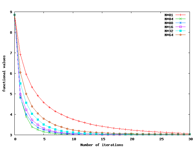
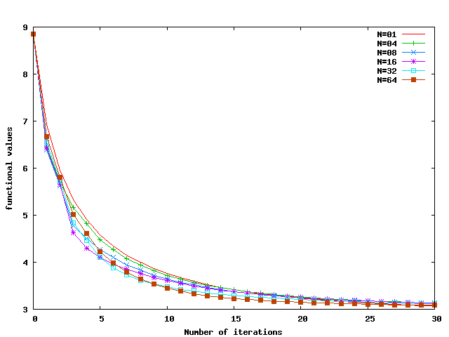
Figure 1. Decaying cost functional values according to the iterations count with respect to sitpoc algorithm (left) and pitpoc algorithm (right).

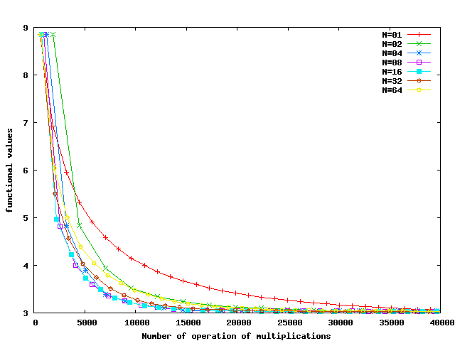
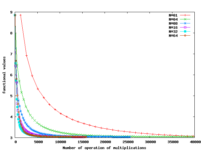
Figure 2. Decaying cost functional values according to the multiplication operations count with respect to sitpoc algorithm (left) and pitpoc algorithm (right).

We first note that Algorithm 4 actually acts as a preconditioner, since it improves the convergence rate of the optimization process. The introduceion of the intermediates targets allows to accelerate the decrease of the functional values, as shown in Figure 2 (left). Note that this property holds mostly for small numbers of sub-intervals, and disapears when dealing with large subdivisions. This feature is lost when considering Algorithm 5, whose convergence does not significantly depend on the number of sub-intervals that is considered, see Figure 2 (right).

On the contrary, Algorithm 5 achieves a good acceleration when considering the number of mutliplications involved in the computations. The corresponding results are shown in Figure 2, where the parallel operations have been counted only once. We see that Algorithm is close to the full efficiency, since the number of multiplications required to obtain a given value for the cost functional is roughly proportional to $\frac{1}{N}$.

We finally consider the wall-clock time required to carry out our algorithms. As the main part of the operations involved in the computation consists in matrix multiplications, the results we present in Figure 3 are close to the ones of Figure 2.

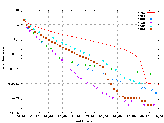
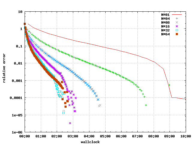
Figure 3. Decaying cost functional values according to elapsed real time with respect to sitpoc algorithm (left) and pitpoc algorithm (right).

8.3. Influence of the number of steps in the optimization method

We now vary the number of steps of the gradient method used in Step II of our algorithm. The results are presented in Figure 4. Subdivisions of $N=4$ and $N=16$ intervals are considered. In both cases, we see that an increase in the number of gradient steps improves the preconditionning feature of our algorithm. However, we also observe that this strategy saturates for large numbers of gradient steps which probably reveals that the sub-problems considered in Step II are practically solved after 5 sub-iterations.

More results can be found in [10].

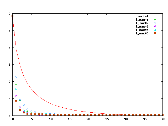
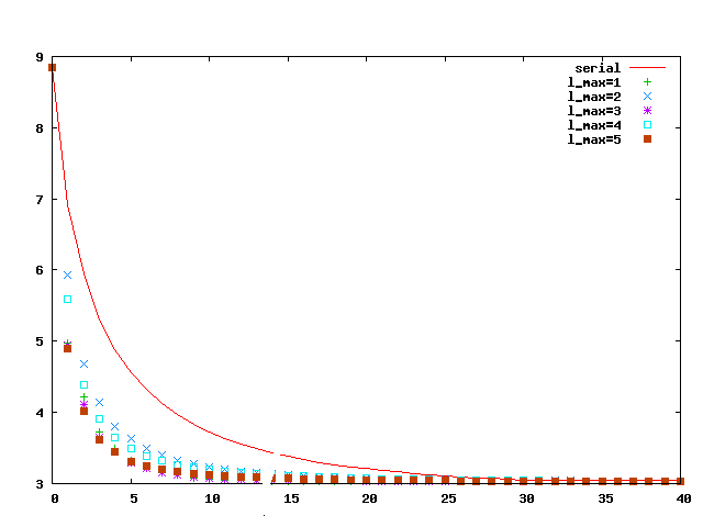
Figure 4. sitpoc algorithm with 4 subdivisions (left) and $16$ subdivision (right): variation of the number of (lower/local)inner-iterations $\ell_{\text{max}}$.

Appendix

For the sake of completeness, we recall here the proof of Lemma 3.
Because of (4.1) and thanks to Young’s inequality, one has for all $t\in[0,T]$ and all $\varepsilon>0$:

$$\frac{1}{2}\frac{d}{dt}\|\delta y(t)\|_{\Omega}^{2}+\nu\|\nabla_{x}\delta y(t)\|_{\Omega}^{2} = \int_{\Omega}\delta y(t)\cal B\delta v(t)dt$$ (8.1)

$$\leq \frac{1}{2}\left(\varepsilon\|\delta y(t)\|_{\Omega}^{2}+\frac{1}{\varepsilon}\|\cal B\delta v(t)\|_{v}^{2}\right),$$

where $\nabla_{x}$ denotes the gradient with respect to the space variable. As $\delta y$ is supposed to satisfies Dirichlet conditions, one can apply Poincaré’s inequality to obtain:

$$\|\delta y(t)\|_{\Omega}\leq C\|\nabla_{x}\delta y(t)\|_{\Omega},$$

for a given $C>0$. Combining this last estimate with (8.1), one gets:

$$\frac{1}{2}\frac{d}{dt}\|\delta y(t)\|_{\Omega}^{2}\leq\left(\frac{\varepsilon}{2}-\frac{\nu}{C^{2}}\right)\|\delta y(t)\|_{\Omega}^{2}+\frac{1}{2\varepsilon}\|\cal B\delta v(t)\|_{v}^{2}.$$

Now, setting $\varepsilon=\frac{2\nu}{C^{2}}$ gives:

$$\frac{d}{dt}\|\delta y(t)\|_{\Omega}^{2}\leq\frac{1}{\varepsilon}\|\cal B\delta v(t)\|_{v}^{2}.$$

Since $\|\delta y(0)\|_{\Omega}^{2}=0$, the result follows with the fact that $\|\cal B\|_{2}\leq 1$.

References

• [1] G. Bal and Y. Maday A parareal time discretization for non-linear PDEs with application to the pricing of an american put, Springer,Lect Notes Comput. Sci. Eng. , 189-202, 2002.
• [2] A. Bellen and M. Zennaro Parallel algorithms for initial value problems for nonlinear vector difference and differential equations, J. Comput. Appl. Math., 25, 341-350, 1989.
• [3] K. Burrage, Parallel and sequential methods for ordinary differential equations, Numerical Mathematics and Scientific Computation, Oxford Science Publications, The Clarendon Press, Oxford University Press, New York, 1995.
• [4] J.-L. Lions, Virtual and effective control for distributed systems and decomposition of everything, J. Anal. Math. 80, 257-297 , 2000.
• [5] J.-L. Lions, Y. Maday and G Turinici, Résolution d’EDP par un shéma pararréel, C. R. Acad. Sci. Paris, I 332 , 661-668, 2001.
• [6] Y. Maday, J. Salomon and G. Turinici, Parareal in time control for quantum systems, SIAM J. Num. Anal., 45 (6), 2468-2482, 2007.
• [7] Y. Maday and G. Turinici, A parareal in time procedure for the control of partial differential equations, C. R. Math. Acad. Sci. Paris 335, 4, 387-392, 2002.
• [8] T. P. Mathew, M. Sarkis and C. E. Schaerer, Analysis of block parareal preconditioners for parabolic optimal control problems, SIAM J. Sci. Comp., 32 (3), 1180-1200, 2010.
• [9] O. Pironneau, F. Hecht and K. Ohtsuka, Free soft : FreeFem++-mpi , http://www.freefem.org.
• [10] M.-K. Riahi, Thèse de doctorat de l’université Pierre et Marie Curie, Paris6, Submitted in december 06, 2011.