Critical slowing down exponents in quenched disordered spin models for structural glasses: Random Orthogonal and related models

Abstract

An important prediction of Mode-Coupling-Theory (MCT) is the relationship between the power-law decay exponents in the $\beta$ regime. In the original structural glass context this relationship follows from the MCT equations that are obtained making rather uncontrolled approximations and $\lambda$ has to be treated like a tunable parameter. It is known that a certain class of mean-field spin-glass models is exactly described by MCT equations. In this context, the physical meaning of the so called parameter exponent $\lambda$ has recently been unveiled, giving a method to compute it exactly in a static framework. In this paper we exploit this new technique to compute the critical slowing down exponents in a class of mean-field Ising spin-glass models including, as special cases, the Sherrington-Kirkpatrick model, the $p$-spin model and the Random Orthogonal model.

I Introduction and framework

It is well known that mean-field spin-glass models have a low temperature phase in which the Replica Symmetry is broken, with a breaking pattern that depends on the specific model. The models displaying a static discontinuous transition which are consistently described by a finite number of breakings are characterized by critical slowing down and a dynamical transition at a temperature higher than the static one.

They share some relevant properties of structural glasses Kirkpatrick and Wolynes (1987a); Kirkpatrick and Thirumalai (1987a, b); Kirkpatrick and Wolynes (1987b), more specifically, the dynamical equations are exactly equivalent to those predicted by the Mode Coupling Theory (MCT) above the mode coupling temperature $T_{mct}$ where ergodicity breaking occurs.
The time autocorrelation function in the high temperature phase displays a fast decay to a plateau and then a second relaxation to equilibrium. Approaching the dynamical transition temperature (called $T_{d}$ in the spin-glass context) the length of the plateau grows progressively until it diverges exactly at $T_{d}$, where the system remains stuck forever in one of the most excited metastable states in a complex free energy landscape. According to MCT the approach to the plateau and the decay from it are both characterized by a power-law behaviour, respectively

$$C(t)\simeq q_{d}+ct^{-a}$$ (1)

$$C(t)\simeq q_{d}-c^{\prime}t^{b}$$ (2)

where $q_{d}$ is the height of the plateau and the two exponents satisfy the following relation that is exact in the framework of MCT (see for example Gotze (2009))

$$\frac{\Gamma^{2}(1-a)}{\Gamma(1-2a)}=\frac{\Gamma^{2}(1+b)}{\Gamma(1+2b)}=\lambda$$ (3)

This relation has been proven to be robust under higher order corrections to standard MCT Andreanov et al. (2009). The exponent parameter $\lambda$ and, consequently, the exponents $a$ and $b$ have been computed exactly only for the spherical $p$-spin model Crisanti et al. (1993) since the dynamical equations are particularly simple and correspond to the so called schematic MCT models.
In most of the cases it is, instead, simply considered a tunable parameter, generically connected to the static structure function at $T_{d}$ through an often explicitly unknown functional Weysser et al. (2010). In the case of continuous transitions, instead, there is no dynamic arrest preceeding the static transition, the time correlation function does not display the two step relaxation and, consequently, no exponent $b$ is defined. At the thermodynamic transition, for long times, the correlation decays to the equilibrium value $q_{EA}$ with a power-law of the kind $C(t)\simeq q_{EA}+ct^{-a}$. The equilibrium order parameter $q_{EA}$ is zero at the transition in absence of magnetic field.
It has been recently pointed out Caltagirone et al. (2012) that there exists a connection between the exponent parameter and the static Gibbs free energy, which allows to compute $\lambda$ in a completely thermodynamic framework, even in cases which go beyond schematic MCT. In the following we will briefly summarize the method.

Given a fully-connected model it is possible to compute the Gibbs free energy $\Gamma(Q)$ as a function of the order parameter that, in the case of a spin-glass transition is the well known overlap matrix $Q$. The value of the order parameter can be determined through a saddle point calculation and $\Gamma(Q)$ can then be expanded around this solution. For our “dynamic” purposes, the expansion has to be performed around a replica symmetric saddle point solution $Q^{SP}_{ab}=q^{SP}$. This gives raise to eight different kinds of third order terms, but only two of them will be relevant, namely:

$$w_{1}\text{Tr}(\delta Q^{3})=w_{1}\sum_{a,b,c}\delta Q_{ab}\delta Q_{bc}\delta Q_{ca}$$ (4)

and

$$w_{2}\sum_{a,b}\delta Q_{ab}^{3}$$ (5)

In the case of discontinuous transitions it can be shown Caltagirone et al. (2012) that the following relation holds at the dynamical transition, giving the connection between the dynamical exponents $a$ and $b$ and the static coefficients, namely

$$\lambda=\frac{w_{2}(T_{d})}{w_{1}(T_{d})}$$ (6)

where $\lambda$ is given in Eq. (3) the expansion of the Gibbs free energy has to be performed around the value of the overlap yelding the height of the plateau at the dynamical transition, $q_{d}$.

Since the coefficients have to be computed at the dynamical transition, where quantities at infinite time do not relax to their equilibrium (thermodynamic) value but remain stuck at their value inside the most excited metastable states, the averages should then be computed inside a single state. This corresponds to taking a 1-RSB Ansatz with breaking parameter $m\rightarrow 1$ or, equivalently, a RS Ansatz with the number of replicas $n\rightarrow 1$ Crisanti (2008); Monasson (1995); Franz and Parisi (1995); Franz et al. (2011).
In this paper we will use the second strategy which is technically much simpler than the first one, therefore we cannot treat the case of a dynamical transition in presence of a magnetic field, since the mutual overlap ($q_{0}$) between states is non-zero and the 1-RSB ($m\rightarrow 1$)/RS ($n\rightarrow 1$) equivalence does not hold.

On the other hand, for continuous transitions a relation between the exponent $a$ and the two coefficients $w_{1}$ and $w_{2}$ analogous to Eq. (6) holds at the static point:

$$\lambda=\frac{w_{2}(T_{s})}{w_{1}(T_{s})}$$ (7)

In this case, since the continuous static transition coincides with the dynamical one (e.g. in the SK model), the dynamical quantities at infinite time relax to their static value Sompolinsky and Zippelius (1982) and the averages can be computed in a replica symmetric Ansatz taking finally the limit $n\rightarrow 0$. For this reason, if the transition is continuous, the RS Ansatz will be sufficient to treat the case in presence of a magnetic field.

In order to compute the two coefficients $w_{1}$ and $w_{2}$ one must determine the expression of the Gibbs free energy as a function of the overlap and then expand it to third order around the RS thermodynamic value $q$. In fully connected models, introducing a replicated external field $\varepsilon$, the free energy reads

$$\begin{split}f(\varepsilon)=-\frac{1}{\beta nN}\ln\int dQ\exp N\left(\SS[Q]+\text{Tr}\,\varepsilon Q\right)\end{split}$$ (8)

which, for $N\rightarrow\infty$, can be evaluated at the saddle point

$$\begin{split}f(\varepsilon)=-\frac{1}{\beta n}\mathrm{extr}_{Q}\left(\SS[Q]+\text{Tr}\,\varepsilon Q\right)\end{split}$$ (9)

We can immediately notice that the equation above exactly defines $f(\varepsilon)$ as the Anti Legendre Transform of the effective action

$$\begin{split}f(\varepsilon)=\mathrm{ALT}\,\SS[Q]\end{split}$$ (10)

and, again, by definition the Gibbs free energy $\Gamma(Q)$ is the Legendre Transform of $f(\varepsilon)$, yelding

$$\begin{split}\Gamma(Q)\equiv\mathrm{LT}\,f(\varepsilon)=\mathrm{LT}\,\left(\mathrm{ALT}\,\SS[Q]\right)=\SS[Q]\end{split}$$ (11)

This implies that the functional form of the Gibbs free energy is equal to the one of the effective action. In fully connected models, we can then directly expand the latter. The general form of the third order term in the free energy is

$$\SS^{(3)}=\sum_{(ab)(cd)(ef)}W_{ab,cd,ef}\,\delta Q_{ab}\delta Q_{cd}\delta Q_{ef}$$ (12)

with

$$W_{ab,cd,ef}=\frac{\partial^{3}\SS(Q)}{\partial Q_{ab}\partial Q_{cd}\partial Q_{ef}}$$ (13)

Since $a\neq b$, $c\neq d$ and $e\neq f$ and the coefficients $W$ are computed in RS Ansatz, we can have eight different vertices. It can be shown Temesvári et al. (2002); Ferrari et al. (2012) that, restricting the variations to the replicon subspace, i.e. the subspace where $\sum_{b}\delta Q^{R}_{ab}=0$, one obtains the following expression containing only the two interesting coefficients $w_{1}$ and $w_{2}$:

$$\begin{split}&\SS^{(3)}_{R}=\sum_{(ab)(cd)(ef)}W_{ab,cd,ef}\,\delta Q^{R}_{ab}\delta Q^{R}_{cd}\delta Q^{R}_{ef}=\\ &=w_{1}\sum_{abc}\delta Q^{R}_{ab}\delta Q^{R}_{bc}\delta Q^{R}_{ca}+w_{2}\sum_{ab}(\delta Q^{R}_{ab})^{3}\end{split}$$ (14)

that follows quite straightforwardly from equation (12) applying the replicon constraint to the variations.
In this paper we apply this technique to study the critical slowing down of a general model of mean-field Ising sping-glass which includes, as particular cases, the SK model, the $p$-spin model and the Random Orthogonal model (ROM). The outline of the paper is the following: in section II we introduce the general model, in section III we give the details of the computation of the parameter exponent $\lambda$ for the general case and briefly present the result for the SK model and $p$-spin model. In section IV we compute $\lambda$ for the ROM model and compare our exact result with numerical simulations. Finally, in section V we give our conclusions and remarks.

II The general model

In this section we will consider a class of mean-field models with Hamiltonian

$${\cal H}=-\sum_{i<j}J_{ij}\sigma_{i}\sigma_{j}-\sum_{p}\sqrt{\frac{R^{(p)}}{p!}}\sum_{i_{1}<\dots<i_{p}}K^{p}_{i_{1},\dots,i_{p}}\sigma_{i_{1}}\cdots\sigma_{i_{p}}$$ (15)

where $\sigma_{i}$ are $N$ Ising spins. The $2$-body interaction matrix is constructed in the following way Cherrier et al. (2003):

$$J={\cal O}^{T}\Xi{\cal O},$$ (16)

where ${\cal O}$ is a random $O(N)$ matrix chosen with the Haar measure. On the other hand, $\Xi$ is a diagonal matrix with elements independently chosen from a distribution $\rho(\xi)$. In order to ensure the existence of the thermodynamic limit, the support of $\rho(\xi)$ must be finite and independent of $N$. The $p$-body interactions $K^{p}$ are i.i.d. gaussian variables with variance

$$\frac{p!}{N^{p-1}}$$ (17)

and

$$R^{(p)}=\frac{d^{p}R}{dx^{p}}(x)\Big{|}_{x=0}$$ (18)

for some real valued function $R$. As shown in Marinari et al. (1994); Cherrier et al. (2003); Crisanti and Sommers (1992) for this class of mean field spin-glasses, the general form of the replicated free energy is:

$$-n\beta f=\mathrm{extr}_{Q,\Lambda}\SS[Q,\Lambda]$$ (19)

with

$$\begin{split}&\SS[Q,\Lambda]=\frac{1}{2}\text{Tr}\,G(\beta Q)+\frac{\beta^{2}}{2}\sum_{ab}\,R(Q_{ab})\\ &-\frac{1}{2}\text{Tr}\,Q\Lambda+\ln\left[\text{Tr}_{\sigma_{a}}\,\exp\left(\frac{1}{2}\sum_{a,b}\Lambda_{ab}\,\,\sigma_{a}\sigma_{b}\right)\right]\end{split}$$ (20)

where $G:\,M_{n\times n}\rightarrow M_{n\times n}$ is a (in general rather complicated) function in the space of $n\times n$ matrices, formally defined through its power series around zero. The particular form of $G$ depends on the choice of the eigenvalue distribution $\rho(\xi)$. In the following we will consider mainly two cases: Wigner law and bimodal.
Given this effective action, the saddle point equations in $\Lambda$ and $Q$ respectively read

$$\begin{split}Q_{ab}&=\langle\langle\sigma_{a}\sigma_{b}\rangle\rangle\\ \Lambda_{ab}&=\beta[G^{\prime}(\beta Q)]_{ab}+\beta^{2}R^{\prime}(Q_{ab})\end{split}$$ (21)

where the average $\langle\langle\cdot\rangle\rangle$ is computed with the measure

$${\cal W}(\Lambda,\sigma)=\frac{e^{\frac{1}{2}\sum_{a,b}\Lambda_{a,b}\sigma_{a}\sigma_{b}}}{\text{Tr}_{\sigma}\,e^{\frac{1}{2}\sum_{a,b}\Lambda_{a,b}\sigma_{a}\sigma_{b}}}$$ (22)

In Replica Symmetric Ansatz ($Q_{ab}=q\,\,,\,\Lambda_{ab}=\hat{\lambda}$ for $a\neq b$ and $Q_{aa}=q_{d}\,\,,\,\Lambda_{aa}=\hat{\lambda}_{d}$), Eq.s (21) become

$$q = \langle m^{2}\rangle$$ (23)

$$\hat{\lambda} = \frac{\beta}{n}[G^{\prime}(\beta(1+(n-1)q))-G^{\prime}(\beta(1-q))]+\beta^{2}R^{\prime}(q)$$

where $m=\tanh(z)$ and the average $\langle\cdot\rangle$ is computed with the measure

$$\mu(\hat{\lambda})=e^{-\frac{z^{2}}{2\hat{\lambda}}}\cosh^{n}(z)\frac{e^{-n\hat{\lambda}/2}}{(2\pi\hat{\lambda})^{1/2}}$$ (24)

In the next section we study in detail the (dynamical) critical behaviour of this class of models and we show how to compute the critical slowing down exponents.

III Computation of the MCT exponents

As explained in the Introduction, in order to compute the parameter exponent $\lambda$ we have to expand the effective action to third order in $Q$ and then restrict the variations to the replicon subspace, obtaining straightforwardly the two coefficients $w_{1}$ and $w_{2}$.

In the present case, the effective action contains the auxiliary field $\Lambda$ which will be eliminated making use of the saddle point equation (21). The expansion of Eq. (20) to third order gives:

$$\begin{split}\delta\SS[Q,\Lambda]\simeq&\frac{1}{2}\text{Tr}[\beta G^{\prime}(\beta Q^{SP})\delta Q+\frac{1}{2}\beta^{2}G^{(2)}(\beta Q^{SP})\delta Q\delta Q+\frac{1}{3!}\beta^{3}G^{(3)}(\beta Q^{SP})\delta Q\delta Q\delta Q]+\\ &+\frac{\beta^{2}}{2}\sum_{ab}[R^{\prime}(Q^{SP}_{ab})\delta Q_{ab}+\frac{1}{2}R^{(2)}(Q^{SP}_{ab})\delta Q_{ab}^{2}+\frac{1}{3!}R^{(3)}(Q^{SP}_{ab})\delta Q_{ab}^{3}]-\\ &-\frac{1}{2}\text{Tr}[Q^{SP}\delta\Lambda+\Lambda^{SP}\delta Q+\delta\Lambda\delta Q]+\frac{1}{2}\sum_{ab}\langle\langle\sigma^{a}\sigma^{b}\rangle\rangle\delta\Lambda_{ab}+\\ &+\frac{1}{2\cdot 4}\sum_{ab,cd}\langle\langle\sigma^{a}\sigma^{b}\sigma^{c}\sigma^{d}\rangle\rangle_{C}\delta\Lambda_{ab}\delta\Lambda_{cd}+\frac{1}{3!\cdot 8}\sum_{ab,cd,ef}\langle\langle\sigma^{a}\sigma^{b}\sigma^{c}\sigma^{d}\sigma^{e}\sigma^{f}\rangle\rangle_{C}\delta\Lambda_{ab}\delta\Lambda_{cd}d\Lambda_{ef}\end{split}$$ (25)

A comment is needed for the first line of eq. (25): the “scalar like” Taylor expansion of a matrix functional $f(M)$, $f:\,\,M_{n\times n}\rightarrow M_{n\times n}$ around some $M_{0}$ (different from the null matrix), is correct only if $[M_{0},\delta M]=0$.

In the present case $Q^{SP}$ is replica symmetric while $\delta Q$ is, in principle, simply symmetric. The commutation condition for a RS matrix with a symmetric matrix reads:

$$\sum_{c}\delta Q_{cb}=\sum_{c}\delta Q_{ac}\,\,\,\,\forall\,a,b$$ (26)

that is satisfied in any subspace orthogonal to the anomalous one (see Temesvári et al. (2002)), i.e. both in the longitudinal and in the replicon sector . Equating to zero the first order of Eq. (25) we obtain the saddle point equations (23).

Considering that the variations $\delta Q$ and $\delta\Lambda$ are in the replicon subspace the second order term simplifies as follows

$$\begin{split}&[\beta^{2}(g^{(2)}_{d}-g^{(2)})+\beta^{2}r^{(2)}]\sum_{ab}\delta Q_{ab}^{2}\\ &-2\sum_{ab}\delta\Lambda_{ab}\delta Q_{ab}+\langle(1-m^{2})^{2}\rangle\sum_{ab}\delta\Lambda_{ab}^{2}\end{split}$$ (27)

where, here and in the following formulas we define the four constants (two diagonal and two off-diagonal):

$$g^{(k)}_{d} = \frac{(n-1)G^{(k)}\left(\beta(1-q)\right)+G^{(k)}\left(\beta(1+(n-1)q)\right)}{n}$$

$$g^{(k)} = \frac{G^{(k)}\left(\beta(1+(n-1)q)\right)-G^{(k)}\left(\beta(1-q)\right)}{n}$$ (28)

$$r^{(k)}_{d} = R^{(k)}(1)$$

$$r^{(k)} = R^{(k)}(q)$$

and

$$\begin{split}G^{(k)}(x)&=\frac{d^{k}G(x)}{dx^{k}}\\ R^{(k)}(x)&=\frac{d^{k}R(x)}{dx^{k}}\end{split}$$ (29)

For the system to be critical, the replicon eigenvalue must vanish and, consequently, the Hessian determinant must be zero.

Imposing this condition we get the following equality

$$\begin{split}\langle(1-m^{2})^{2}\rangle=\frac{1}{[\beta^{2}(g^{(2)}_{d}-g^{(2)})+\beta^{2}r^{(2)}]}\end{split}$$ (30)

Eq. (30) together with Eq.s (23) gives the criticality condition, which locates the dynamical or static transition point depending on the value ($n=1,0$) of the replica number.

Now we want to eliminate the auxiliary field. The $\Lambda$ - saddle point equation (21) reads (up to second order)

$$\begin{split}\delta Q_{ab}&=\frac{1}{2}\sum_{cd}\langle\langle\sigma^{a}\sigma^{b}\sigma^{c}\sigma^{d}\rangle\rangle_{C}\delta\Lambda_{cd}\\ &+\frac{1}{4}\sum_{cd,ef}\langle\langle\sigma^{a}\sigma^{b}\sigma^{c}\sigma^{d}\sigma^{e}\sigma^{f}\rangle\rangle_{C}\delta\Lambda_{cd}d\Lambda_{ef}\end{split}$$ (31)

Exploiting the property of the replicon subspace and the criticality condition we can write the variation in the following way:

$$\begin{split}\delta Q_{ab}&=\langle(1-m^{2})^{2}\rangle\delta\Lambda_{ab}\\ &+\langle(1-m^{2})^{3}\rangle\sum_{c}\delta\Lambda_{ac}\delta\Lambda_{cb}\\ &+2\langle m^{2}(1-m^{2})^{2}\rangle\delta\Lambda_{ab}^{2}\end{split}$$ (32)

Inverting the equation we obtain

$$\begin{split}\delta\Lambda_{ab}&=[\beta^{2}(g^{(2)}_{d}-g^{(2)})+\beta^{2}r^{(2)}]\delta Q_{ab}\\ &-[\beta^{2}(g^{(2)}_{d}-g^{(2)})+\beta^{2}r^{(2)}]^{3}\times\\ &\Bigl{(}\langle(1-m^{2})^{3}\rangle\sum_{c}\delta Q_{ac}\delta Q_{cb}+\\ &2\langle m^{2}(1-m^{2})^{2}\rangle\delta Q_{ab}^{2}\Bigr{)}\end{split}$$ (33)

Now we define

$$\begin{split}&{\cal C}_{1}\equiv\langle(1-m^{2})^{3}\rangle\\ &{\cal C}_{2}\equiv 2\langle m^{2}(1-m^{2})^{2}\rangle\end{split}$$ (34)

and plug the constraint (33) into (25), obtaining three different contributions to the third order in $\delta Q$, namely

$$\begin{split}&-\frac{1}{2}\text{Tr}[\delta\Lambda\delta Q]\rightarrow\\ &\qquad\qquad\frac{1}{2}[\beta^{2}(g^{(2)}_{d}-g^{(2)})+\beta^{2}r^{(2)}]^{3}\times\\ &\qquad\qquad\Big{(}{\cal C}_{1}\delta Q_{ab}\sum_{c}\delta Q_{bc}\delta Q_{ca}+{\cal C}_{2}\delta Q_{ab}^{3}\Big{)}\\ \end{split}$$ (35)

$$\begin{split}&\frac{1}{2\cdot 4}(2M_{1}-4M_{2}+2M_{3})\sum_{ab}\delta\Lambda_{ab}^{2}\rightarrow\\ &\qquad\qquad-\frac{1}{2}[\beta^{2}(g^{(2)}_{d}-g^{(2)})+\beta^{2}r^{(2)}]^{3}\times\\ &\qquad\qquad\Big{(}{\cal C}_{1}\delta Q_{ab}\sum_{c}\delta Q_{bc}\delta Q_{ca}+{\cal C}_{2}\delta Q_{ab}^{3}\Big{)}\\ \end{split}$$ (36)

$$\begin{split}&\frac{1}{3!\cdot 8}\sum_{ab,cd,ef}\langle\langle\sigma^{a}\sigma^{b}\sigma^{c}\sigma^{d}\sigma^{e}\sigma^{f}\rangle\rangle_{C}\delta\Lambda_{ab}\delta\Lambda_{cd}d\Lambda_{ef}\rightarrow\\ &\qquad\qquad\frac{1}{3!}[\beta^{2}(g^{(2)}_{d}-g^{(2)})+\beta^{2}r^{(2)}]^{3}\times\\ &\qquad\qquad\Big{(}{\cal C}_{1}\sum_{abc}\delta Q_{ab}\delta Q_{bc}\delta Q_{ca}+{\cal C}_{2}\sum_{ab}\delta Q_{ab}^{3}\Big{)}\end{split}$$ (37)

Summing all the third order contributions in Eq. (25), we eventually find

$$\begin{split}w_{1}&=\frac{1}{2}\frac{\beta^{3}}{3!}(g^{(3)}_{d}-g^{(3)})+\frac{1}{3!}[\beta^{2}(g^{(2)}_{d}-g^{(2)})+\beta^{2}r^{(2)}]^{3}{\cal C}_{1}\\ w_{2}&=\frac{1}{2}\frac{\beta^{2}}{3!}r^{(3)}+\frac{1}{3!}[\beta^{2}(g^{(2)}_{d}-g^{(2)})+\beta^{2}r^{(2)}]^{3}{\cal C}_{2}\end{split}$$ (38)

Substituting Eq. (III) one immediately obtains a general expression for the exponent parameter, that is the main result of this paper:

$$\begin{split}&\lambda=\frac{w_{2}}{w_{1}}=\frac{R^{(3)}(q)+2\beta^{4}\mathcal{D}(\beta,q)^{3}\,{\cal C}_{2}}{\beta G^{(3)}(\beta(1-q))+2\beta^{4}\mathcal{D}(\beta,q)^{3}\,{\cal C}_{1}}\end{split}$$ (39)

where

$$\mathcal{D}(\beta,q)\equiv G^{(2)}(\beta(1-q))+R^{(2)}(q)$$ (40)

III.1 SK model on the dAT line

The Sherrington - Kirkpatrick model Sherrington and Kirkpatrick (1975) is described by the Hamiltonian

$${\cal H}=-\frac{1}{2}\sum_{ij}J_{ij}\sigma_{i}\sigma_{j}-H\sum_{i}\sigma_{i}$$ (41)

where the couplings are i.i.d. random variables distributed according to a gaussian with zero mean and variance $1/N$. This model belongs to the class defined above, with $R=x^{2}/2$ and $G=0$ or, conversely, $R=0$ and $G=x^{2}/2$ Sherrington and Kirkpatrick (1975), except for the presence of the magnetic field term. We will see in a while that this affects the result in a very simple way.
It is well known that in the SK model there exists a line of instability of the replica symmetric solution in the $\beta-H$ plane, the de Almeida - Thouless (dAT) line de Almeida and Thouless (1978), where the so called replicon eigenvalue of the stability matrix vanishes. In this section we want to compute the decay exponent of the time correlation function along this line. In order to get the result we first have to find solutions which satisfy simultaneously the saddle point and the dAT equations, respectively

$$q=\int d\mu(z)\tanh^{2}(\beta\sqrt{q}z+\beta H)$$ (42)

$$\begin{split}&1=\beta^{2}\int d\mu(z)\,\mathrm{sech}^{4}(\beta\sqrt{q}z+\beta H)\\ &d\mu(z)=\frac{1}{\sqrt{2\pi}}e^{-\frac{z^{2}}{2}}\end{split}$$ (43)

Notice that the expression (39) is completely general and holds for every model belonging to this class, while the details of the model enter in the specific form of the functions $G$ and $R$. In the case of continuous transitions, the presence of the magnetic field, only modifies the definition of the parameter $m$ in equation (39) which becomes:

$$m=\tanh(z+\beta H)$$ (44)

without changing the formal expression for the coefficients. Therefore, plugging into the effective action (20) $R(x)=\frac{1}{2}x^{2}$ so that $R^{(2)}(x)=1$ and $R^{(3)}(x)=0$. Then we get immediately the expression for the exponent parameter:

$$\lambda=\frac{{\cal C}_{2}}{{\cal C}_{1}}\equiv\frac{2\left\langle m^{2}(1-m^{2})^{2}\right\rangle}{\langle(1-m^{2})^{3}\rangle}$$ (45)

Our result exactly coincides with the one obtained by Sompolinsky and Zippelius Sompolinsky and Zippelius (1982) in a purely dynamical framework.

III.2 Multi p-spin Ising model

Starting from an Hamiltonian of the kind of Eq. (15) without the first term, leads to a generalized version of the $p$-spin model Gardner (1985), in wich many multibody interaction terms are considered, depending on the actual form of the function $R$. As shown in refs Crisanti and Leuzzi (2004, 2007); Crisanti et al. (2011), in these models, the thermodynamic properties, the critical dynamics and replica symmetry breaking structure depend on the relative strength of the coupling terms (the coefficients of the expansion of $R$). Indeed, in order to treat a particular case, before applying our technique, one should understand the behavior of the corresponding model.

The simple $p$-spin Ising model is characterized by $R(x)=ax^{p}$, where a $a\neq 1$ affects only the variance of the couplings distribution and indeed rescales the temperature. For $p>2$, in absence of any external magnetic field, the model displays a standard RFOT transition from the paramagnetic RS phase to the 1-RSB spin-glass and, at a lower temperature, a second transition to a FRSB spin-glass Gardner (1985). Focusing on the first transition, we can compute the critical dynamic exponents in the present general framework while a specific analysis was presented by some of us in Ferrari et al. (2012). In order to recover the exact same model, we have to set $R(x)=x^{p}/2$, which reduces Eq.(23) and (30) to:

$$\begin{split}q&=\langle m^{2}\rangle\\ \hat{\lambda}&=\frac{p\beta^{2}}{2}q^{p-1}\\ 1&=\frac{p(p-1)\beta^{2}q^{p-2}}{2}\langle(1-m^{2})^{2}\rangle\end{split}$$ (46)

and Eq. (39) to:

$$\begin{split}\lambda=\frac{2\left\langle m^{2}(1-m^{2})^{2}\right\rangle+\frac{2(p-2)q^{3-2p}}{\beta^{4}p^{2}(p-1)^{2}}}{\left\langle(1-m^{2})^{3}\right\rangle}\end{split}$$ (47)

as it was found in Ferrari et al. (2012).

IV Random Orthogonal Model

The Random Orthogonal Model (ROM) Marinari et al. (1994); Cherrier et al. (2003) is obtained with the choice $R=0$ and

$$\rho(\xi)=\alpha\,\delta(\xi-1)+(1-\alpha)\,\delta(\xi+1)$$ (48)

It displays a random first order transition regardless of the value of the tunable parameter $\alpha$. The case with $\alpha=1/2$ has been extensively sudied in Marinari et al. (1994) while the general case was treated in Cherrier et al. (2003).
They show that, as a consequence of the choice of the eigenvalue distribution (48), the function $G$ appearing in the effective action reads :

$$\begin{split}2G(x)&=[1+4x(2\alpha-1+x)]^{1/2}\\ &+(2\alpha-1)\ln\{[1+4x(2\alpha-1+x)]^{1/2}+2x+2\alpha-1\}\\ &-\ln\{[1+4x(2\alpha-1+x)]^{1/2}+1+2(2\alpha-1)x\}\\ &-(2\alpha-1)\ln(2\alpha)-1+\ln(2)\end{split}$$ (49)

Using Eq.s (21) we can determine the transition temperature $T_{d}$ and the dynamical overlap $q_{d}$ which are shown in Figs. 1 and 2 and coincide with those found in Ref. Cherrier et al. (2003).

Once the critical point is obtained as a function of $\alpha$, using formula (39) specialized to the ROM case, we obtain the value of the exponent parameter $\lambda(\alpha)$ and of the critical slowing down exponents $a(\alpha)$ and $b(\alpha)$ which are shown in Fig. 3. We find numerically that for $\alpha\rightarrow 1$ the exponent parameter goes to $\lambda=\frac{2}{3}$ as in the Ising $p$-spin model for $p\rightarrow\infty$ Ferrari et al. (2012). On the other hand for $\alpha\rightarrow 0$ we find $\lambda=\frac{1}{2}$ as in the Ising $p$-spin model for $p\rightarrow 2$.

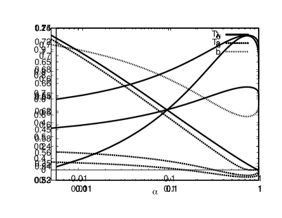
Figure 1: The static and dynamical critical temperature as a function of the parameter $\alpha$.
They both diverge for $\alpha\rightarrow 0$ and are zero at $\alpha=1$.

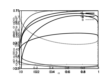
Figure 2: The static and dynamical critical overlap as a function of the parameter $\alpha$.

Figure 3: Solid line: the exponent parameter $\lambda$. Dashed line: the exponent $a$. Dot-dashed line: the exponent $b$.

In particular, for $\alpha=13/32$ we have $b=0.628$. We now use this value to compare with numerical simulations.

IV.1 Comparison with Monte Carlo data

There are recent numerical simulations by Sarlat et al. Sarlat et al. (2009) on the fully connected ROM which give an estimate for the MCT exponents $a$, $b$ and $\gamma$. They choose $\alpha=\frac{13}{32}\simeq 0.4$ in order to have higher transition temperatures and a good separation between the static and dynamical critical temperature.
Their direct estimate of the exponent $b$ is $0.62$, while their direct estimate of $\gamma$ is $2.1$ which, through the exact MCT relations:

$$\begin{split}&\frac{\Gamma^{2}(1+b)}{\Gamma(1+2b)}=\frac{\Gamma^{2}(1-a)}{\Gamma(1-2a)}\\ &\gamma=\frac{1}{2a}+\frac{1}{2b}\end{split}$$ (50)

yields $b_{MCT}\simeq 0.75$.
Our exact computation yields instead $b_{th}\simeq 0.628$, which suggests that the best estimate of the exponent $b$ in Sarlat et al. (2009) is the direct one, that is very close to the actual value.

V Summary and conclusions

In the present work we have introduced a general fully-connected model for Ising spins, which combines an orthogonal two body interaction with a set of $p$-body interactions.

Exploiting a technique that has been recently introduced Caltagirone et al. (2012), based on the equivalence between statics and long time dynamics, we have been able to find an analytic expression for the exponent parameter $\lambda$, in a purely static framework. As particular cases of the general model we have studied the Sherrington-Kirkpatrick model along the de Almeida-Thouless line, the $p$-spin model and the Random Orthogonal model.
For the SK model we find the same result found by Sompolinsky and Zippelius in Ref. Sompolinsky and Zippelius (1982).
For the $p$-spin we recover, as a byproduct of the general model, the results given in detail in ref. Ferrari et al. (2012).
We have studied the critical behaviour of the parameteric class of Random Orthogonal models at arbitrary values of the constant $\alpha\in[0,1]$, that determines the distribution of the eigenvalues of the interaction matrix. The exponent parameter and the two MCT exponents have been determined analitically for any $\alpha$ and in particular we have looked at $\alpha=13/32$ in order to make a comparison with existing numerical simulations Sarlat et al. (2009). Our exact result is in very good agreement with the one obtained in the Monte Carlo study, through a direct estimate of $b$ (late $\beta$ regime).
On the other hand, a direct estimate of the exponent $\gamma$ gives a result that is quite far from what we found here, suggesting that the strong finite-size corrections affect the value of $\gamma$ much more than $b$. Numerical interpolations at criticality are very sensitive for glassy models and the corresponding estimates can strongly suffer of this drawback.

References

- Kirkpatrick and Wolynes (1987a) T. Kirkpatrick and P. Wolynes, Phys. Rev. B 36, 8552 (1987a).
- Kirkpatrick and Thirumalai (1987a) T. Kirkpatrick and D. Thirumalai, Phys. Rev. B 36, 5388 (1987a).
- Kirkpatrick and Thirumalai (1987b) T. Kirkpatrick and D. Thirumalai, Phys. Rev. Lett. 58, 2091 (1987b).
- Kirkpatrick and Wolynes (1987b) T. R. Kirkpatrick and P. G. Wolynes, Phys. Rev. A 35, 3072 (1987b).
- Gotze (2009) W. Gotze, Complex Dynamics of Glass-Forming Liquids: A Mode-Coupling Theory (Oxford University Press, 2009).
- Andreanov et al. (2009) A. Andreanov, B. G., and B. J.-P., EPL 88, 16001 (2009).
- Crisanti et al. (1993) A. Crisanti, H. Horner, and H. Sommers, Z. Phys. B 92, 257 (1993).
- Weysser et al. (2010) F. Weysser, A. M. Puertas, M. Fuchs, and T. Voigtmann, Phys. Rev. E 82, 011504 (2010).
- Caltagirone et al. (2012) F. Caltagirone, U. Ferrari, L. Leuzzi, G. Parisi, F. Ricci-Tersenghi, and T. Rizzo, Phys. Rev. Lett. 108, 085702 (2012).
- Crisanti (2008) A. Crisanti, Nucl. Phys. B 796, 425 (2008).
- Monasson (1995) R. Monasson, Phys. Rev. Lett. 75, 2847 (1995).
- Franz and Parisi (1995) S. Franz and G. Parisi, J. Phys. I (France) 5, 1401 (1995).
- Franz et al. (2011) S. Franz, G. Parisi, F. Ricci-Tersenghi, and T. Rizzo, European Physical Journal E 34, 1 (2011).
- Sompolinsky and Zippelius (1982) H. Sompolinsky and A. Zippelius, Phys. Rev. B 25, 6860 (1982).
- Temesvári et al. (2002) T. Temesvári, C. De Dominicis, and I. Pimentel, The European Physical Journal B 25, 361 (2002).
- Ferrari et al. (2012) U. Ferrari, L. Leuzzi, G. Parisi, and T. Rizzo, arXiv:1202.4168v1 (2012).
- Cherrier et al. (2003) R. Cherrier, D. S. Dean, and A. Lefèvre, Phys. Rev. E 67, 046112 (2003).
- Marinari et al. (1994) E. Marinari, G. Parisi, and F. Ritort, Journal of Physics A: Mathematical and General 27, 7647 (1994).
- Crisanti and Sommers (1992) A. Crisanti and H. Sommers, Z. Phys. B 87, 341 (1992).
- Sherrington and Kirkpatrick (1975) D. Sherrington and T. Kirkpatrick, Phys. Rev. Lett 35, 1792 (1975).
- de Almeida and Thouless (1978) J. R. L. de Almeida and D. J. Thouless, J. Phys. A 11, 983 (1978).
- Gardner (1985) E. Gardner, Nucl. Phys. B 257, 747 (1985).
- Crisanti and Leuzzi (2004) A. Crisanti and L. Leuzzi, Phys. Rev. Lett. 93, 217203 (2004).
- Crisanti and Leuzzi (2007) A. Crisanti and L. Leuzzi, Phys. Rev. B 76, 184417 (2007).
- Crisanti et al. (2011) A. Crisanti, L. Leuzzi, and M. Paoluzzi, Eur. Phys. J. E 34, 98 (2011).
- Sarlat et al. (2009) T. Sarlat, A. Billoire, G. Biroli, and J. P. Bouchaud, J. Stat. Mech. (2009).