Unstable $m=1$ modes of counter–rotating Keplerian discs

Abstract

We study the linear $m=1$ counter-rotating instability in a two–component, nearly Keplerian disc. Our goal is to understand these slow modes in discs orbiting massive black holes in galactic nuclei. They are of interest not only because they are of large spatial scale—and can hence dominate observations—but also because they can be growing modes that are readily excited by accretion events. Self–gravity being nonlocal, the eigenvalue problem results in a pair of coupled integral equations, which we derive for a two-component softened gravity disc. We solve this integral eigenvalue problem numerically for various values of mass fraction in the counter-rotating component. The eigenvalues are in general complex, being real only in the absence of the counter–rotating component, or imaginary when both components have identical surface density profiles. Our main results are as follows: (i) the pattern speed appears to be non negative, with the growth (or damping) rate being larger for larger values of the pattern speed; (ii) for a given value of the pattern speed, the growth (or damping) rate increases as the mass in the counter–rotating component increases; (iii) the number of nodes of the eigenfunctions decreases with increasing pattern speed and growth rate. Observations of lopsided brightness distributions would then be dominated by modes with the least number of nodes, which also possess the largest pattern speeds and growth rates.

1 Introduction

Most galactic nuclei are thought to host massive black holes and dense clusters of stars whose structure and kinematics are correlated with global galaxy properties (Gebhardt et al., 1996; Ferrarese & Merritt, 2000; Gebhardt et al., 2000). Such correlations raise questions of great interest related to galaxy formation and the growth of nuclear black holes. The nearby large spiral galaxy M31 has an off–centered peak in a double–peaked brightness distribution around its nuclear black hole (Light et al., 1974; Lauer et al., 1993, 1998; Kormendy & Bender, 1999). This lopsided brightness distribution could arise naturally if the apoapses of many stellar orbits, orbiting the black hole, happened to be clustered together (Tremaine, 1995). Since then, kinematic and dynamical models of such an eccentric disc have been constructed by several authors (Bacon et al., 2001; Salow & Statler, 2001; Sambhus & Sridhar, 2002; Peiris & Tremaine, 2003). Of particular interest to this work is the model of Sambhus & Sridhar (2002), which included a few per cent of stars on retrograde (i.e. counter–rotating) orbits. They proposed that these stars could have been accreted to the centre of M31 in the form of a globular cluster that spiraled in due to dynamical friction. This proposal was motivated by the work of Touma (2002), who demonstrated that a Keplerian axisymmetric disc is susceptible to a linear lopsided instability in the $m=1$ mode, even when a small fraction of the disc mass is in retrograde motion.

Touma (2002) considered the linearized secular dynamics of particles orbiting a point mass, wherein particle orbits may be thought of as slowly deforming elliptical rings of small eccentricities. The $m=1$ counter–rotating instability was studied analytically for a two–ring system, and numerically for a many–ring system. The corresponding problem for continuous discs was then studied by Sridhar & Saini (2010), who proposed a simple model with dynamics that could be studied largely analytically in the Wentzel–Kramers–Brillouin (WKB) approximation. Their model consisted of a two–component softened gravity disc, orbiting a massive central black hole. Softened gravity was introduced by Miller (1971) to simplify the analysis of the dynamics of stellar systems. In this form of interaction, the Newtonian $1/d$ gravitational potential is replaced by $1/\sqrt{d^{2}+b^{2}}$, where $b>0$ is called the softening length. In the context of waves in discs, it is well known that the softening length mimics the epicyclic radius of stars on nearly circular orbits (Binney & Tremaine, 2008). Therefore, a disc composed of cold collisionless matter, interacting via softened gravity, provides a surrogate for a hot collisionless disc.

Sridhar & Saini (2010) used a short–wavelength (WKB) approximation, derived analytical expressions for the dispersion relation and showed that the frequency $\omega$ is smaller than the Keplerian orbital frequency by a factor proportional to the small quantity $\varepsilon=M_{d}/M\,$ (which is the ratio of the disc mass to mass of the central object); in other words, the modes are slow. The WKB dispersion relation was used to argue that equal mass counter–rotating discs with the same surface density profiles (i.e. when there is not net rotation) could have unstable modes. They also argued that, for an arbitrary mass ratio, the discs must be unrealistically hot to avoid an instability. Sridhar & Saini (2010) then used Bohr–Sommerfeld quantization to construct global modes, within the WKB approximation. A matter of concern is that the wavelengths of the modes could be of order the scale length of the discs; the modes being large–scale it is possible that the WKB approximation itself is invalid. Another limitation is that Sridhar & Saini (2010) could construct (WKB) global modes only for the case of equal mass discs. Therefore it is necessary to address the full eigenvalue problem to understand the systematic behaviour of eigenvalues and eigenfunctions. To this end, we formulate the eigenvalue problem for the linear, slow, $m=1$ modes in a two–component, softened gravity, counter–rotating disc. Due to the long–range nature of gravitational interactions, we have to deal with a pair of coupled integral equations defining the eigenvalue problem. We draw some general conclusions and then proceed to solve the equations numerically for eigenvalues and eigenfunctions.

In § 2 we introduce the unperturbed two–component nearly Keplerian disc, define the apse precession rates, discuss the potential theory for softened gravity, and derive the coupled, linear integral equations that determine the eigenvalue problems for slow $m=1$ modes. A derivation of the relationship between the softened Laplace coefficients (used in the potential theory of § 2 and § 3) and the usual (unsoftened) Laplace coefficients is given in the Appendix. We specialize to discs with similar surface density profiles in § 3, when the two coupled equations can be cast as a single integral equation in a new mode variable; this allows us to draw some general conclusions about the eigenvalue problem. We also discuss in detail the numerical method to be employed. Our results are presented in § 4, where the properties of the stable, unstable and overstable modes are discussed. Conclusions are offered in § 5, where we seek to provide a global perspective on the correlations that occur between the pattern speeds, growth rates and eigenfunctions, as well as the variations of these quantities on the mass fraction in retrograde orbits.

2 Formulation of the linear eigenvalue problem

We consider linear non–axisymmetric perturbations in two counter–rotating discs orbiting a central point mass $M$. The discs are assumed to be coplanar and consist of cold collisionless particles which attract each other through softened gravity. However, the central mass and the disc particles interact via the usual (unsoftened) Newtonian gravity. Softened gravity is known to mimic the effects of velocity dispersion, so our discs are surrogates for hot stellar discs. We assume that the total mass in the discs, $M_{d}$, is small in comparison to the central mass. Since $\varepsilon\equiv M_{d}/M\ll 1$, the dynamics is dominated by the Keplerian attraction of the central mass, and the self–gravity of the discs is a small perturbation which enables slow modes. Below we formulate the linear eigenvalue problem of slow modes.

2.1 Unperturbed discs

We use polar-coordinates $\mathbf{r}\equiv(R\,,\phi)$ in the plane of the discs, with the origin at the location of the central mass. Throughout this paper the superscripts ‘$+$’ and ‘$-$’ refer to the prograde and retrograde components, respectively. The unperturbed discs are assumed to be axisymmetric with surface densities $\Sigma_{d}^{\pm}(R)$. The disc particles orbit in circles with velocities, ${\mathbf{v}}_{d}^{\pm}=\pm\,R\Omega(R){\mathbf{e}}_{\phi}$, where $\Omega(R)>0$ is the angular speed determined by the unperturbed gravitational potential,

$$\Phi(R)\;=\;-\,\frac{GM}{R}\;+\;\Phi_{d}(R)\,.$$ (1)

The first term on the right side is the Keplerian potential due to the central mass, and $\Phi_{d}(R)$ is the softened gravitational potential due to the combined self-gravities of both the discs:

$$\Phi_{d}(\mathbf{r})\;=\;-\,G\int\,\frac{\Sigma_{d}^{+}({\mathbf{r}}^{\prime})+\Sigma_{d}^{-}({\mathbf{r}}^{\prime})}{\sqrt{\left|{\mathbf{r}}\,-\,{\mathbf{r}}^{\prime}\right|^{2}+b^{2}}}\;{\mathrm{d}}^{2}r^{\prime}\,,$$ (2)

where $b$ is the Miller softening length; the potential $\Phi_{d}(R)$ is $O(\epsilon)$ compared to $GM/R$. Test particles for nearly circular prograde orbits have azimuthal and radial frequencies, $\Omega$ and $\kappa$, given by

$$\Omega^{2}(R) \;=\;\frac{GM}{R^{3}}\;+\;\frac{1}{R}\frac{\mbox{${\mathrm{d}}$}{\Phi_{d}}}{\mbox{${\mathrm{d}}$}{R}},$$ (3)

$$\kappa^{2}(R) \;=\;\frac{GM}{R^{3}}\;+\;\frac{3}{R}\frac{\mbox{${\mathrm{d}}$}{\Phi_{d}}}{\mbox{${\mathrm{d}}$}{R}}\;+\;\frac{\mbox{${\mathrm{d}}$}^{2}{\Phi_{d}}}{\mbox{${\mathrm{d}}$}{R}^{2}}\,.$$ (4)

The line of apsides of a nearly circular eccentric particle orbit of angular frequency $\pm\Omega(R)$, subjected only to gravity, precesses at a rate given by $\pm\dot{\varpi}(R)$, where

$$\dot{\varpi}(R) \;=\;\Omega(R)\;-\;\kappa(R)$$

$$\;=\;-\frac{1}{2\Omega(R)}\left(\frac{2}{R}\frac{\mbox{${\mathrm{d}}$}}{\mbox{${\mathrm{d}}$}R}+\frac{\mbox{${\mathrm{d}}$}^{2}{}}{\mbox{${\mathrm{d}}$}{R}^{2}}\right)\Phi_{d}(R)\;+\;O(\varepsilon^{2})\,.$$ (5)

The cancellation of the $O(1)$ term, $(GM/R^{3})$, which is common to both $\Omega^{2}$ and $\kappa^{2}$ makes $\dot{\varpi}\sim O(\varepsilon)$. This is the special feature of nearly Keplerian discs which is responsible for the existence of (slow) modes whose eigenfrequencies are $\sim O(\varepsilon)$ when compared with orbital frequencies.

2.2 Perturbed discs

Let ${\bf{v}}_{a}^{\pm}({\mathbf{r}},t)=u_{a}^{\pm}(\mathbf{r}{}{},t){\mathbf{e}_{R}}+v_{a}^{\pm}(\mathbf{r}{}{},t){\mathbf{e}_{\phi}}$ and $\Sigma_{a}^{\pm}({\mathbf{r}},t)$ be infinitesimal perturbations to the velocity fields and surface densities of the $\pm$ discs, respectively. These satisfy the following linearized Euler and continuity equations:

$$\frac{\partial{{\bf{v}}_{a}^{\pm}}}{\partial{t}}\;+\; ({\bf{v}}_{d}^{\pm}\cdot\nabla){\bf{v}}_{a}^{\pm}\;+\;({\bf{v}}_{a}^{\pm}\cdot\nabla){\bf{v}}_{d}^{\pm}\;=\;-\nabla\Phi_{a}\,,$$ (6)

$$\frac{\partial{\Sigma_{a}^{\pm}}}{\partial{t}}\;+\; \nabla\cdot(\Sigma_{d}^{\pm}{\bf{v}}_{a}^{\pm}\;+\;\Sigma_{a}^{\pm}{\bf{v}}_{d}^{\pm})\;=\;0,$$ (7)

where $\Phi_{a}({\bf{r}},t)$ is the perturbing potential. Fourier analyzing the perturbations in $t$ and $\phi$, we seek solutions of the form, $X_{a}({\mathbf{r}},t)=\sum_{m}X_{a}^{m}(R)\exp[{\rm i}(m\phi-\omega t)]\,$. Then

$$u_{a}^{m\pm}\;=\; -\frac{\rm i}{D_{m}^{\pm}}\left[(\pm m\Omega-\omega)\frac{\mbox{${\mathrm{d}}$}}{\mbox{${\mathrm{d}}$}R}\;\pm\;\frac{2m\Omega}{R}\right]\Phi_{a}^{m}\,,$$ (8)

$$v_{a}^{m\pm}\;=\; \frac{1}{D_{m}^{\pm}}\left[\pm\frac{\kappa^{2}}{2\Omega}\frac{\mbox{${\mathrm{d}}$}}{\mbox{${\mathrm{d}}$}R}\;+\;\frac{m}{R}(\pm m\Omega-\omega)\right]\Phi_{a}^{m}\,,$$ (9)

$${\rm i}(\pm m\Omega- \omega)\Sigma_{a}^{m\pm}\;+\;\frac{1}{R}\frac{\mbox{${\mathrm{d}}$}}{\mbox{${\mathrm{d}}$}R}(R\Sigma_{d}^{\pm}u_{a}^{m\pm})\;+\;\frac{{\rm i}m}{R}\Sigma_{d}^{\pm}v_{a}^{m\pm}=0\,,$$ (10)

where

$$D_{m}^{\pm}\;=\; \kappa^{2}\;-\;(\pm m\Omega-\omega)^{2}\,.$$ (11)

The above equations determine $u_{a}^{m\pm}$, $v_{a}^{m\pm}$ and $\Sigma_{a}^{m\pm}$ in terms of the perturbing potential $\Phi_{a}^{m}\,$; this would be the solution were $\Phi_{a}^{m}$ due to an external source.

We are interested in modes for which $\Phi_{a}^{m}$ arises from self gravity. In this case it depends on the total perturbed surface density, $\left[\Sigma_{a}^{m+}(R)+\Sigma_{a}^{m-}(R)\right]\,$. Manipulating the Poisson integral given in Eq. 2, we obtain

$$\Phi_{a}^{m}(R)\;=\; \int_{0}^{\infty}R^{\prime}{\mathrm{dR^{\prime}}}\,P_{m}(R,R^{\prime})\,[\Sigma_{a}^{m+}(R^{\prime})+\Sigma_{a}^{m-}(R^{\prime})]\,,$$ (12)

where the kernel

$$P_{m}(R,R^{\prime})\;=\; -\frac{\pi G}{R_{>}}B_{1}^{(m)}(\alpha,\beta)\;+\;\frac{\pi GR}{R^{\prime 2}}(\delta_{m,1}+\delta_{m,-1})\,.$$ (13)

The second term on the right side is the indirect term arising from the fact that our coordinate system can be a non–inertial frame, because its origin is located on the central mass. The first term is the direct term coming from the perturbed self–gravity. Here $R_{<}=\min(R,R^{\prime})\,$, $R_{>}=\max(R,R^{\prime})\,$, $\alpha=R_{<}/R_{>}$ and $\beta=b/R_{>}\,$. The functions,

$$B_{s}^{(m)}(\alpha,\beta)\;=\; \frac{2}{\pi}\int_{0}^{\pi}{\mathrm{d\theta}}\,\frac{\cos m\theta}{(1-2\alpha\cos\theta+\alpha^{2}+\beta^{2})^{s/2}}\,,$$ (14)

are “softened Laplace coefficients”, introduced in Touma (2002). They can be expressed in terms of the usual (unsoftened) Laplace coefficients, as shown in Appendix A. We note that the unperturbed disc potential $\Phi_{d}$ can be obtained from the unperturbed disc density, $\Sigma_{d}^{+}(R)+\Sigma_{d}^{-}(R)\,$, by using Eq. (12) with $m=0\,$.

2.3 Slow $m=1$ modes

Modes with azimuthal wavenumber $m=\pm 1$ are slow in the sense that their eigenfrequencies, $\omega$, are smaller than the orbital frequency, $\Omega$, by a factor $\sim O(\varepsilon)\,$. Without loss of generality we may choose $m=1$. In the slow mode approximation (Tremaine, 2001), we use the fact that $\Omega\gg\omega$ in Eqs. (8)—(11), and write

$$u_{a}^{1\pm}\;=\; \mp\,\frac{\rm i}{D_{1}^{\pm}}\left[\Omega\frac{\mbox{${\mathrm{d}}$}}{\mbox{${\mathrm{d}}$}R}\;+\;\frac{2\Omega}{R}\right]\Phi_{a}^{1}\,,$$ (15)

$$v_{a}^{1\pm}\;=\; \pm\,\frac{1}{D_{1}^{\pm}}\left[\frac{\Omega}{2}\frac{\mbox{${\mathrm{d}}$}}{\mbox{${\mathrm{d}}$}R}\;+\;\frac{\Omega}{R}\right]\Phi_{a}^{1}\,,$$ (16)

$$\pm\,{\rm i}\,\Omega\Sigma_{a}^{1\pm}\;+\; \frac{1}{R}\frac{\mbox{${\mathrm{d}}$}}{\mbox{${\mathrm{d}}$}R}(R\Sigma_{d}^{\pm}u_{a}^{1\pm})\;+\;\frac{\rm i}{R}\Sigma_{d}^{\pm}v_{a}^{1\pm}\;=\;0\,,$$ (17)

where

$$D_{1}^{\pm}\;=\; \pm 2\Omega(\omega\;\mp\;\dot{\varpi}).$$ (18)

Eqs. (15) and (16) imply the following relations between the perturbed velocity amplitudes:

$$u_{a}^{1\pm}\;=\; -2{\rm i}v_{a}^{1\pm}\,,$$

$$D_{1}^{-}u_{a}^{1-}\;=\; -D_{1}^{+}u_{a}^{1+}\,,$$

$$D_{1}^{-}v_{a}^{1-}\;=\; -D_{1}^{+}v_{a}^{1+}\,.$$ (19)

We use Eqs. (19) in the continuity equation (17) to eliminate $u_{a}^{1\pm}$ and write,

$$\pm\,\Omega\Sigma_{a}^{1\pm}\;=\;\frac{2}{R^{1/2}}\frac{\mbox{${\mathrm{d}}$}}{\mbox{${\mathrm{d}}$}R}(R^{1/2}\Sigma_{d}^{\pm}{v}_{a}^{1{\pm}})\,.$$ (20)

Combining Eqs. (12), (16) and (18)—(20) we obtain

$$\left[\omega\;\mp\;\dot{\varpi}(R)\right]{v}_{a}^{1{\pm}}(R)\;=\; \int_{0}^{\infty}\frac{{\mathrm{d}R^{\prime}}\,R^{\prime 1/2}}{2R^{2}\Omega(R^{\prime})}\,\left\{\frac{\partial{}}{\partial{R}}\left[R^{2}P_{1}(R,R^{\prime})\right]\right\}\times$$

$$\quad\left\{\frac{\mbox{${\mathrm{d}}$}{}}{\mbox{${\mathrm{d}}$}{{R^{\prime}}}}\left[R^{\prime 1/2}\Sigma_{d}^{+}(R^{\prime}){v}_{a}^{1{+}}(R^{\prime})\;-\;R^{\prime 1/2}\Sigma_{d}^{-}(R^{\prime}){v}_{a}^{1{-}}(R^{\prime})\right]\right\}\,.$$ (21)

We rewrite this by defining

$$z^{\pm}(R)\;=\;\left[\frac{R^{2}\Sigma_{d}^{\pm}(R)}{\Omega(R)}\right]^{1/2}\,{v}_{a}^{1{\pm}}\,,$$ (22)

use the fact that $\Omega(R)\propto R^{-3/2}$ for a Keplerian flow, and integrate by parts to obtain,

$$\left[\omega\;\mp\;\dot{\varpi}(R)\right]z^{\pm}(R)\;=\; -\int_{0}^{\infty}\frac{{\mathrm{d}}R^{\prime}}{R^{\prime}}\,2\mathcal{F}(R,R^{\prime})\left[\frac{\Sigma_{d}^{+}(R^{\prime})\Sigma_{d}^{\pm}(R)}{\Omega(R^{\prime})\Omega(R)}\right]^{1/2}z^{+}(R^{\prime})$$

$$+\,\,\int_{0}^{\infty}\frac{{\mathrm{d}}R^{\prime}}{R^{\prime}}\,2\mathcal{F}(R,R^{\prime})\left[\frac{\Sigma_{d}^{-}(R^{\prime})\Sigma_{d}^{\pm}(R)}{\Omega(R^{\prime})\Omega(R)}\right]^{1/2}z^{-}(R^{\prime})\,,$$ (23)

where

$$\mathcal{F}(R,R^{\prime})\;=\;\left(1+\frac{1}{2}\frac{\partial{}}{\partial{\,\ln R^{\prime}}}\right)\left(1+\frac{1}{2}\frac{\partial{}}{\partial{\,\ln R}}\right)P_{1}(R,R^{\prime})\,.$$ (24)

It is convenient to write $\Sigma_{d}^{-}(R)=\eta(R)\Sigma_{d}(R)$ and $\Sigma_{d}^{+}(R)=(1-\eta(R))\Sigma_{d}(R)\,$, where $\eta(R)$ is the local mass fraction in the unperturbed counter-rotating component; by definition, $0\leq\eta(R)\leq 1$. Then, Eq. $(\ref{eq:per15})$ can be recast as

$$\omega z^{+}(R)\;=\;+\dot{\varpi}z^{+}(R)\;+\; \int_{0}^{\infty}\frac{{\mathrm{d}}R^{\prime}}{R^{\prime}}[(1-\eta(R^{\prime}))(1-\eta(R))]^{1/2}\mathcal{K}(R,R^{\prime})z^{+}(R^{\prime})$$

$$-\; \int_{0}^{\infty}\frac{{\mathrm{d}}R^{\prime}}{R^{\prime}}[\eta(R^{\prime})(1-\eta(R))]^{1/2}\mathcal{K}(R,R^{\prime})z^{-}(R^{\prime})\,,$$

$$\omega z^{-}(R)\;=\;-\dot{\varpi}z^{-}(R)\;+\; \int_{0}^{\infty}\frac{{\mathrm{d}}R^{\prime}}{R^{\prime}}[(1-\eta(R^{\prime}))\eta(R)]^{1/2}\mathcal{K}(R,R^{\prime})z^{+}(R^{\prime})$$

$$-\; \int_{0}^{\infty}\frac{{\mathrm{d}}R^{\prime}}{R^{\prime}}[\eta(R^{\prime})\eta(R)]^{1/2}\mathcal{K}(R,R^{\prime})z^{-}(R^{\prime}),$$ (25)

where the kernel

$$\mathcal{K}(R,R^{\prime})\;=\; -\,2\left[\frac{\Sigma_{d}(R^{\prime})\Sigma_{d}(R)}{\Omega(R^{\prime})\Omega(R)}\right]^{1/2}\,\mathcal{F}(R,R^{\prime})$$

$$\;=\; -\,2\left[\frac{\Sigma_{d}(R^{\prime})\Sigma_{d}(R)}{\Omega(R^{\prime})\Omega(R)}\right]^{1/2}\,\left(1+\frac{1}{2}\frac{\partial{}}{\partial{\,\ln R^{\prime}}}\right)\left(1+\frac{1}{2}\frac{\partial{}}{\partial{\,\ln R}}\right)P_{1}(R,R^{\prime})$$

$$\;=\; 2\pi G\left[\frac{\Sigma_{d}(R^{\prime})\Sigma_{d}(R)}{\Omega(R^{\prime})\Omega(R)}\right]^{1/2}\,\left(1+\frac{1}{2}\frac{\partial{}}{\partial{\,\ln R^{\prime}}}\right)\left(1+\frac{1}{2}\frac{\partial{}}{\partial{\,\ln R}}\right)\frac{B_{1}^{(1)}(\alpha,\beta)}{R_{>}}\,.$$ (26)

Therefore the kernel $\mathcal{K}(R,R^{\prime})$ is a real symmetric function of $R$ and $R^{\prime}$.

Using Eqs. (19) and (22), we can relate the eigenfunctions $z^{+}(R)$ and $z^{-}(R)$ to each other:

$$\sqrt{(1-\eta(R))}\left[\omega-\dot{\varpi}(R)\right]z^{+}(R)\;=\;\sqrt{\eta(R)}\left[\omega+\dot{\varpi}(R)\right]z^{-}(R)\,.$$ (27)

This relation can, in principle, be used to eliminate one of $z^{+}(R)$ or $z^{-}(R)$ from the coupled Eqs. (25), in which case the eigenvalue problem can be formulated in terms of a single function (which can be either $z^{+}(R)$ or $z^{-}(R)$). However, such a procedure results in a further complication: the eigenvalue, $\omega$, will then occur inside the $R^{\prime}$ integral in the combination, $(\omega\pm\dot{\varpi})/(\omega\mp\dot{\varpi})$, and this makes further analysis difficult. Eqs. (25) are symmetric under the (simultaneous) transformations, $\left\{`+^{\prime}\,,\eta(R)\,,\omega\,\right\}\;\to\;\left\{`-^{\prime}\,,\left[1-\eta(R)\right]\,,-\omega\,\right\}$, which interchange the meanings of the terms prograde and retrograde. It seems difficult to obtain general results when $\Sigma_{d}^{+}(R)$ and $\Sigma_{d}^{-}(R)$ have different functional forms. Below we consider the case when the mass fraction, $\eta$, is a constant; i.e. when both $\Sigma_{d}^{+}(R)$ and $\Sigma_{d}^{-}(R)$ have the same radial profile.

3 The eigenvalue problem for constant $\eta$ discs

When the counter–rotating discs have the same unperturbed surface density profiles, i.e. $\Sigma_{d}^{+}(R)\propto\Sigma_{d}^{-}(R)\,$, some general results can be obtained. This case corresponds to the choice $\eta=\mbox{constant}$, so that $\Sigma_{d}^{-}(R)=\eta\Sigma_{d}(R)$ and $\Sigma_{d}^{+}(R)=(1-\eta)\Sigma_{d}(R)\,$. Then the eigenfunctions $z^{+}(R)$ and $z^{-}(R)$ are related to each other by,

$$\left[\omega-\dot{\varpi}(R)\right]\sqrt{\eta}\,z^{+}(R)\;=\;\left[\omega+\dot{\varpi}(R)\right]\sqrt{(1-\eta)}\,z^{-}(R)\,.$$ (28)

Let us define a new function, $Z(R)$, which is a linear combination of $z^{+}(R)$ and $z^{-}(R)\,$:

$$Z(R)\;=\;\sqrt{1-\eta}\,z^{+}(R)\;-\;\sqrt{\eta}\,z^{-}(R)\,.$$ (29)

Then equations (25) can be manipulated to derive a closed equation for $Z(R)\,$:

$$\left[\frac{\omega^{2}-\dot{\varpi}^{2}}{(1-2\eta)\omega+\dot{\varpi}}\right]\,Z(R)\;=\;\int_{0}^{\infty}\frac{\mathrm{d}R^{\prime}}{R^{\prime}}\,\mathcal{K}(R,R^{\prime})\,Z(R^{\prime})\,,$$ (30)

We note that, in this integral eigenvalue problem for the single unknown function $Z(R)\,$, the (as yet undetermined) eigenvalue $\omega$ occurs outside the integral. Once the problem is solved and $Z(R)$ has been determined, we can use Eq. (28) and (29) to recover $z^{\pm}(R)\,$:

$$z^{+}(R)\;=\;\sqrt{1-\eta}\,\frac{\omega+\dot{\varpi}(R)}{(1-2\eta)\omega+\dot{\varpi}}\,Z(R)\,,\qquad z^{-}(R)\;=\;\sqrt{\eta}\,\frac{\omega-\dot{\varpi}(R)}{(1-2\eta)\omega+\dot{\varpi}}\,Z(R)\,.$$ (31)

Some general conclusions can be drawn:

1. In Eq. (30), the kernel $\mathcal{K}(R,R^{\prime})$ is real symmetric. Therefore, the eigenvalues, $\omega$, are either real or come in complex conjugate pairs.

2. When $\eta=0$, the counter–rotating component is absent, which is the case studied by Tremaine (2001); then the left side of Eq. (30) becomes $\left(\omega-\dot{\varpi}\right)Z\,$. Since the kernel $\mathcal{K}(R,R^{\prime})$ is real symmetric, the eigenvalues $\omega$ are real, so the slow modes are stable and oscillatory in time. Then the eigenfunctions, $Z(R)$ may be taken to be real. Therefore $z^{+}(R)=Z(R)$ is a real function, and $z^{-}(R)=0\,$.

3. When $\eta=1/2\,$, there is equal mass in the counter–rotating component, and the surface densities of the $\pm$ discs are identical to each other. This case may also be thought of as one in which there is no net rotation at any radius. Then Eq. (30) becomes

   $$\dot{\varpi}^{-1}(R)\left(\omega^{2}-\dot{\varpi}^{2}(R)\right)Z(R)\;=\;\int_{0}^{\infty}\frac{\mathrm{d}R^{\prime}}{R^{\prime}}\,\mathcal{K}(R,R^{\prime})\,Z(R^{\prime})\,,$$ (32)

   Since the kernel $\mathcal{K}(R,R^{\prime})$ is real symmetric, $\omega^{2}$ must be real. There are two cases to consider, when the eigenvalues, $\omega$, are either real or purely imaginary.

   $\bullet$ When $\omega$ is real, the slow modes are stable and oscillatory in time. The eigenfunctions $z^{\pm}(R)$ can be taken to be real functions.

   $\bullet$ When $\omega$ is imaginary, the eigenvalues come in pairs that are complex conjugates of each other, corresponding to non–oscillatory growing/damped modes. Let us set $\eta=1/2$ and $\omega=\rm i\gamma\,$ (where $\gamma$ is real) in Eq. (31):

   $$z^{+}(R)\;=\;\frac{\rm i\gamma+\dot{\varpi}(R)}{2^{1/2}\dot{\varpi}(R)}\,Z(R)\,,\qquad\qquad z^{-}(R)\;=\;\frac{\rm i\gamma-\dot{\varpi}(R)}{2^{1/2}\dot{\varpi}(R)}\,Z(R)$$ (33)

   The function $Z(R)$, which is a solution of Eq. (32), can be taken to be a real function multiplied by an arbitrary complex constant. It is useful to note two special cases: (i) when $Z(R)$ is purely imaginary, then $z^{+}(R)$ and $z^{-}(R)$ are complex conjugates of each other; (ii) when $Z(R)$ is real, $z^{+}(R)$ is equal to minus one times the complex conjugate of $z^{-}(R)$.

To make progress for other values of $\eta$, it seems necessary to address the eigenvalue problem numerically; the rest of this paper is devoted to this.

3.1 Application to Kuzmin discs

For numerical explorations of the eigenvalue problem, we consider the case when both the unperturbed $\pm$ discs are Kuzmin discs, with similar surface density profiles: $\Sigma_{d}^{-}(R)=\eta\Sigma_{d}(R)$ and $\Sigma_{d}^{+}(R)=(1-\eta)\Sigma_{d}(R)\,$, where

$$\Sigma_{d}(R)\;=\;\frac{aM_{d}}{2\pi(R^{2}+a^{2})^{3/2}}$$ (34)

is the total surface density, $M_{d}$ is the total disc mass and $a$ is the disc scale length. Kuzmin discs, being centrally concentrated, are reasonable candidates for unperturbed discs. Moreover, earlier investigations of slow modes (Tremaine, 2001; Sridhar & Saini, 2010) have explored modes in Kuzmin discs, so we find this choice useful for comparisons with earlier work. The characteristic values of orbital frequency and surface density are given by $\Omega^{\star}=\sqrt{{GM}/{a^{3}}}$, and $\Sigma_{d}^{*}={M_{d}}/{a^{2}}$, respectively. The coupled Eqs.  (25) can be cast in a dimensionless form in terms of these physical scales. The net effect is to rescale the eigenvalue $\omega$ to $\sigma$, where

$$\sigma=\left(\frac{\Omega^{\star}a}{G\Sigma^{\star}}\right)\omega\,.$$ (35)

In the following section, all quantities are to be taken as dimensionless; however, with some abuse of notation, we shall continue to use the same symbols for them.

3.2 Numerical method

Our method is broadly similar to Tremaine (2001). In order to calculate eigenvalues and eigenfunctions numerically, we approximate the integrals by a discrete sum using an $N$–point quadrature rule. The presence of the term ${\mathrm{dR}}/R$ in the integrals suggests that a natural choice of variables is $u=\log(R)$ and $v=\log(R^{\prime})$, where, as mentioned above, $R$ stands for the dimensionless length $R/a$. The use of a logarithmic scale is numerically more efficient, because it induces spacing in the coordinate space that increases with the radius. This handles naturally a certain expected behaviour of the eigenfunctions: since the surface density in a Kuzmin disc is a rapidly decreasing function of the radial distance, we expect the eigenfunctions to also decrease rapidly with increasing radius. Therefore, discretization of the coupled equations (25) follows the schema:

$$\int_{0}^{\infty}\frac{\mathrm{d}R^{\prime}}{R^{\prime}}\,\mathcal{K}(R,R^{\prime})\,z^{+}(R^{\prime})\quad\longrightarrow\quad\sum_{i=1}^{N}w_{i}\,\mathcal{K}(e^{u},e^{v_{i}})\,z^{+}(e^{v_{i}})\,,$$ (36)

where $w_{i}$’s are suitably chosen weights. Then the discretized equations can be written as a matrix eigenvalue problem:

$$\bf{A}\,\zeta\;=\;\sigma\,\zeta\,,$$ (37)

where

$$\bf{A}\;=\;\left[\begin{array}[]{cc}(1-\eta)w_{j}{\mathcal{K}}_{ij}+\dot{\varpi}_{j}\delta_{ij}&\quad-\sqrt{\eta(1-\eta)}w_{j}{\mathcal{K}}_{ij}\\[10.00002pt] \sqrt{\eta(1-\eta)}w_{j}{\mathcal{K}}_{ij}&\quad-\eta w_{j}{\mathcal{K}}_{ij}-\dot{\varpi}_{j}\delta_{ij}\end{array}\right]\,,\qquad\mbox{and}\qquad\bf{\zeta}\;=\;\left(\begin{array}[]{c}z^{+}_{i}\\[10.00002pt] z^{-}_{i}\end{array}\right)\,.$$ (38)

The $2N\,\times\,2N$ matrix $\bf{A}$ has been represented above in a $2\,\times\,2$ block form, where each of the 4 blocks is a $N\,\times\,N$ matrix, with row and column indices $i$ and $j$. Note that $\delta_{ij}$ is the Kronecker delta symbol, and no summation is implied over the repeated $j$ indices. Thus we have an eigenvalue problem for eigenvalues $\sigma$, and eigenvectors given by the $2N$ dimensional column vector $\zeta\,$. The use of unequal weights destroys the natural symmetry of the kernel, but this is readily restored through a simple transformation given in § 8.1 of Press et al. (1992). The grid for our numerical calculations covers the range $-7\leq\log R\leq 5$, which is divided into $N=4000$ points; larger values of $N$ give similar results.

We note some differences with Tremaine (2001) concerning details of the numerical method and assumptions. The major difference is in the treatment of softening: In Tremaine (2001), a dimensionless softening parameter $\beta=b/R\,$ was introduced, and the eigenvalue problem for slow modes was solved by holding the parameter $\beta$ constant, This renders the physical softening length, $b$, effectively dependent on radius, making it larger at larger radii, thereby not corresponding to any simple force law between two disc particles located at different radii. We have preferred to keep $b$ constant, so that the force law between two disc particles is through the usual Miller prescription. Other minor differences in treatment are: (i) in Tremaine (2001), the disc interior to an inner cut-off radius was assumed to be frozen. In contrast we use a straightforward inner cut-off radius of $10^{-5}\,$, as mentioned above; (ii) Tremaine (2001) uses a uniform grid in $\log R$, with four–point quadrature in the intervals between consecutive grid points; we also use a uniform grid in $\log R$ but instead employ a single $N$–point quadrature for integration.

Were we dealing with unsoftened gravity (i.e. the case when $b=0\,$), the diagonal elements of the kernel would be singular. Hence, when the softening parameter $b$ is much smaller than the grid size, accuracy is seriously compromised by round-off errors. Typically, the usable lower limit for $b$ is $\sim 10^{-2}$.

Figure 1: Slow g–modes in a single, prograde ($\eta=0$) Kuzmin disc with $\lambda=0.1$ and $b=10^{-2}$. The panels are labeled by the scaled eigenvalue $\sigma$.

Figure 2: Slow p–modes in single, prograde ($\eta=0$) Kuzmin disc with no external source (i.e $\lambda=1$). The panels are labeled by the scaled eigenvalue $\sigma$, and the softening parameter, $b$ (which has been scaled with respect to $a$, the disc scale length).

Figure 3: Growth rate versus number of nodes for $\eta=0.5$, for two values of softening, $b=0.1$ and $b=0.05$.

Figure 4: Eigenfunctions $Z(R)$ are plotted as a function of the radial coordinate $R$, for $\eta=0.5\,$. The panels are labeled by the values of the growth rate, $\Gamma$, and softening, $b$.

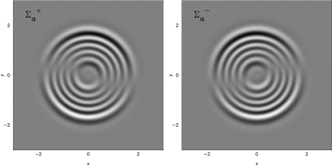
Figure 5: Gray–scale plots of surface density perturbations, $\Sigma_{a}^{\pm}(R,\phi,t)$ at time $t=0$ for the parameter values, $\eta=0.5\,$ and $b=0.1\,$, and $\Gamma=0.0230$. White/black correspond to the maximum positive/negative values of the perturbations.

4 Numerical results

We obtained the eigenvalues and eigenfunctions of equation (37) using the linear algebra package LAPACK (Anderson et al., 1999). We now present the results of our calculations for specific values of $\eta$. As noted earlier, interchanging the meaning of prograde and retrograde orbits leave the results invariant under the transformation $(\eta,\omega)\to(1-\eta\,,-\omega)$; therefore, we present results below only for $0\leq\eta\leq 1/2\,$.

4.1 No counter-rotation: $\eta=0$

We are dealing with a single disc whose particles rotate in the prograde sense. The eigenvalue problem for this case was studied first by Tremaine (2001), who also showed that the eigenvalues are real; in other words, the disc supports stable slow modes. We consider this case first to benchmark our numerical method as well as assess the differences in results that may arise due to the manner in which softening is treated. To facilitate comparison we use the same nomenclature as Tremaine (2001). Briefly, modes corresponding to positive and negative eigenvalues are referred to as “p–modes” and “g-modes”, respectively; we also introduce a parameter $\lambda=(1+f)^{-1}$, where $f$ is a constant that mimics additional precession due to an external source of the form $\dot{\varpi}_{e}(R)=f\dot{\varpi}_{d}(R)$; we define eccentricity ${\rm e}_{K}$ through

$${\rm e}_{K}\;=\;2\,\left(\frac{GM}{R}\right)^{-1/2}{v}_{a}^{1{}}\,,$$ (39)

and use the normalization,

$$\int\frac{\mathrm{d}\mathrm{R}}{R}\,{\rm e}_{K}^{2}(R)\;=\;1\,.$$ (40)

Our results corresponding to g–modes, for $\lambda=0.1$ and $\beta=10^{-2}$, are presented in Fig. 1, where we plot modes with three or fewer nodes and give their eigenvalues. Results for p–modes for $\lambda=1$ (no external source) and various values of softening parameter $b$, are displayed in Fig. 2. These figures are to be compared with Fig. 3 and Fig. 6 of Tremaine (2001): the eigenfunctions are of broadly similar form, but the eigenvalues differ from those in Tremaine (2001) by upto $\sim 30\%\,$.

4.2 Equal counter-rotation (or no net rotation): $\eta=1/2$

This case was studied by Sridhar & Saini (2010), who derived the following local or “WKB” dispersion relation:

$$\omega^{2}=\dot{\varpi}\left(\dot{\varpi}+\frac{\pi G\Sigma_{d}(R)}{\Omega(R)}|k|\exp(-|k|b)\right)\,.$$ (41)

From this expression they concluded: if $\dot{\varpi}$ happens to be positive then $\omega$ is real (and the disc is stable), but $\dot{\varpi}$ is negative for most continuous discs which implies that $\omega$ can be either real or purely imaginary. Sridhar & Saini (2010) also studied global modes using Bohr–Sommerfeld quantization, which will be discussed later in this section.

We have proved in the last section that the eigenvalues are either real (stable oscillatory modes), or purely imaginary (non–oscillatory growing and damped modes). Here we focus on the growing (unstable) modes; we define the growth rate of perturbations as,

$$\Gamma=\sqrt{\frac{4}{3}}b|\sigma|\,.$$ (42)

in order to facilitate comparisons with Sridhar & Saini (2010). In Fig. 3, we plot $\Gamma$ for $b$ equal to $0.1$ and $0.05$, versus the number of nodes of $Z(R)$. Sridhar & Saini (2010) found two separate branches in the spectrum, corresponding to long and short wavelengths (for each value of $b$). Comparing our Fig.  3 with their Figs. 3 & 4, we see that our results are more consistent with their short–wavelength branch than with their long–wavelength branch. This disagreement is probably because the long–wavelength branch corresponds to $kR\sim 1$, where WKB approximation breaks down. Moreover, the agreement between our results and their short–wavelength branch holds only in a broad sense, because there are differences in the numerical values of the eigenvalues. We trace this difference to the fact that Sridhar & Saini (2010) used an analytical result for the precession frequency corresponding to unsoftened gravity, whereas we have consistently used softened gravity for all gravitational interactions between disc particles. This probably also results in another difference between our results: according to Sridhar & Saini (2010), $10^{-3}<\Gamma<10^{-2}$; however, as can be seen from our Fig. 3, we obtain values of $\Gamma$ both inside and outside this range. Changing the value of $b$ causes a horizontal shift in the spectrum, which is consistent with their results.

In Fig 4, we plot a few of these eigenfunctions as a function of $R$ for both values of $b$ equal to $0.1$ and $0.05$. Note that, from the discussion in the previous section, $Z(R)$ can always be chosen to be a real function of $R$. The smallest number of nodes corresponds to the largest value of the growth factor. The eigenfunctions with the fewest nodes have significant amplitudes in a small range of radii around $R\sim 1$, and this range increases with the number of nodes (and correspondingly, the growth rate decreases). Fig 5 is a gray–scale plot of the surface density perturbations in the $\pm$ discs, $\Sigma_{a}^{\pm}(R,\phi,t=0)$. Note the relative phase shift between the $\pm$ perturbations. For other value of $b$ shown in Fig 4 we get similar patterns.

Figure 6: Distribution of eigenvalues in the complex $\sigma$ plane, for $\eta=0.1,0.25$ and $0.4$. Panels labeled $\mathnormal{a}$ give an overview, whereas the panels labeled $\mathnormal{b}$ provide an close–up view near the origin.

Figure 7: Real parts of the “most unstable” eigenfunctions $Z(R)$, plotted as a function of the radial coordinate, $R$ for $b=0.1$ and for $\eta=0.1,0.25$ and $0.4$. Panels are labeled by the real and imaginary parts of the eigenvalues.

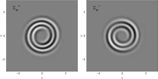
Figure 8: Gray–scale plots of surface density perturbations, $\Sigma_{a}^{\pm}(R,\phi,t)$ at time $t=0$ for the parameter values, $\eta=0.25\,$ and $b=0.1\,$, and $\sigma=0.1408+\rm i0.2332$. White/black correspond to the maximum positive/negative values of the perturbations.

Figure 9: Real parts of two pairs of eigenfunctions $Z(R)$ (from two arms of a branch), plotted as a function of the radial coordinate $R$, for $b=0.1$ and $\eta=0.25$. Panels are labeled by the real and imaginary parts of the eigenvalues.

4.3 Other values of $\eta$

We present results for values of $\eta$ other than $0$ and $1/2$. These are particularly interesting, not only because they were not explored by Sridhar & Saini (2010), but because the eigenvalues can be truly complex, corresponding to growing and damped modes which precess with steady pattern speeds. We write the eigenvalues as $\sigma=\sigma_{\mathnormal{R}}+\rm i\sigma_{\mathnormal{I}}$. In Fig 6, we display the eigenvalues in the complex $\sigma$–plane, for softening parameter $b=0.1$ and for $\eta$ equal to $0.1$, $0.25$ and $0.4$. Panels on the left, labeled $(\mathnormal{a})$, provide an overview, whereas the panels on the right, labeled $(\mathnormal{b})$, provide a close–up view of the distribution of eigenvalues near the origin of the complex $\sigma$–plane; this distribution is similar to Fig. 3 of Touma (2002). We are able to provide much more detail, essentially because we are dealing with continuous discs rather than a finite number of rings.

As $\eta$ increases from $0$, the eigenvalues go from real to complex, a bifurcation that has been traced in Touma (2002) to a phenomenon identified by M. J. Krein due to the resonant crossing of stable modes. The complex eigenvalues come in complex conjugate pairs, so there are two branches to the distribution. As $\eta$ increases, the branches progressively separate and, for $\eta=1/2$ must lie along the positive and negative imaginary axes. It is intriguing that each of these two branches consists of more than one arm. In the close–up views provided by the $(\mathnormal{b})$ panels, it appears as if each of the branches has two arms; however, more detailed investigations are required to determine if there are more arms. The arms of each of the branches are most widely separated when $\eta=0.25$, which is the value of $\eta$ exactly midway in its range $0\leq\eta\leq 0.5\,$. The separations decrease as $\eta$ approaches either $0$ or $1/2$; this is natural because, for $\eta=0$ both branches must lie on the real axis and, for $\eta=1/2$ both branches must lie on the imaginary axis.

The eigenfunctions are in general complex, and have a rich structure as functions of their eigenvalues. Since our interest is in the unstable modes, we now display in Fig. 7 plots of the $Z_{R}=\Re[Z(R)]$ in Eq. (29), corresponding to the “most unstable” modes (for softening parameter $b=0.1$ and for $\eta$ equal to $0.1$, $0.25$ and $0.4$). In other words, for some chosen value of $\sigma_{R}$, we display the real part of the eigenfunction corresponding to the largest value of $\sigma_{\mathnormal{I}}$. For a fixed value of $\eta$, the number of nodes of the eigenfunctions decreases with increasing pattern speed and growth rate. Fig 8 is a gray–scale plot of the surface density perturbations in the $\pm$ discs, $\Sigma_{a}^{\pm}(R,\phi,t=0)$, for the parameter values $\eta=0.25$ and $b=0.1$, and $\sigma=0.1408+\rm i0.2332$ .

It is also of interest to ask how eigenfunctions from two different arms of the same branch behave. To do this, we picked two eigenfunctions with nearly the same value of $\sigma_{R}$, but with values of $\sigma_{I}$ corresponding to two different arms of one branch; Fig. 9 shows two such pairs of eigenfunctions for $\eta=0.25$. We have looked at pairs of such eigenfunctions for other values of $\eta$, but do not display them, here we note what seems to be a general trend: (i) the two members of a pair are more similar to each other when the values of their $\sigma_{R}$ are closer to each other; (ii) the member of a pair with the smaller value of $\sigma_{I}$ is more displaced toward larger radii.

5 Conclusions

We study linear, slow $m=1$ modes in softened gravity, counter–rotating Keplerian discs. The eigenvalue problem is formulated as a pair of coupled integral equations for the $\pm$ modes. We then specialize to the case when the two discs have similar surface density profiles but different $\pm$ disc masses. It is of great interest to study the properties of the modes as a function of $\eta$, which is the fraction of the total disc mass in the retrograde population. Recasting the coupled equations as a single equation in a new modal variable, we are able to demonstrate some general properties: for instance, when $\eta=1/2$, the eigenvalues must be purely imaginary or, equivalently, the modes are purely unstable. In other words, when the $\pm$ discs have identical surface density profiles then there are growing $m=1$ modes with zero pattern speed, a conclusion which is consistent with Araki (1987); Palmer & Papaloizou (1990); Sellwood & Merritt (1994); Lovelace et al. (1997); Touma (2002); Tremaine (2005). To study modes for general values of $\eta$, the eigenvalue problem needs to be solved numerically. Our method is broadly based on Tremaine (2001), but there are some differences whose details have been discussed in the text. The main point of departure is in the way that softening has been treated. In Tremaine (2001), a dimensionless softening parameter $\beta=b/R\,$ was introduced, and the eigenvalue problem was solved by holding the parameter $\beta$ constant. This procedure renders the physical softening length, $b$, effectively dependent on radius (making it larger at larger radii), thereby not corresponding to any simple force law between two disc particles located at different radii. We have preferred to keep $b$ constant, so that the force law between two disc particles is through the usual Miller prescription.

We calculate eigenvalues and eigenfunctions numerically for discs with surface density profiles of Kuzmin form. Kuzmin discs, being centrally concentrated, are reasonable candidates for unperturbed discs. Moreover, earlier investigations of slow modes (Tremaine, 2001; Sridhar & Saini, 2010) have explored modes in Kuzmin discs, so this choice is particularly useful for comparisons with earlier work. Comparing our results with those of Tremaine (2001) for $\eta=0$ (when the slow modes are stable), we find that the eigenfunctions are of broadly similar form, but the eigenvalues differ by up to $\sim 30\%\,$; this is a result of the different ways in which we have treated softening. For the case of no net rotation ($\eta=1/2$), we find that the growth rates (of the unstable modes) we calculate are broadly consistent with the short–wavelength branch of the global WKB modes determined earlier by Sridhar & Saini (2010), but not their long–wavelength branch. This disagreement probably arises because the long–wavelength branch corresponds to wavelengths of order the disc scale length where WKB approximation breaks down. Moreover, the agreement between our results and their short–wavelength branch holds only in a broad sense, because there are differences in the numerical values of the eigenvalues. We trace this difference to the fact that Sridhar & Saini (2010) used an analytical result for the precession frequency corresponding to unsoftened gravity, whereas we have consistently used softened gravity for all gravitational interactions between disc particles.

We have also investigate eigenmodes for values of $\eta$ other than $0$ and $1/2$. These cases are particularly interesting, not only because they were not explored by Sridhar & Saini (2010), but because the eigenvalues can be truly complex, corresponding to growing (and damped) modes with non zero pattern speeds. We have presented results for $\eta=0.1,0.25$ and $0.4$ in the previous sections. Based on these, we interpolate and offer the following conclusions about the properties of the eigenmodes and their physical implications, for all values of $\eta$ (which is the mass fraction in the retrograde population):

1. For a general value of $\eta$ (between $0$ and $1/2$), the distribution of eigenvalues in the complex plane has two branches. These branches are symmetrically placed about the real axis, because the eigenvalues come in complex conjugate pairs.

2. The pattern speed appears to be non negative for all values of $\eta$, with the growth (or damping) rate being larger for larger values of the pattern speed.

3. For a fixed value of $\eta$, the number of nodes of the eigenfunctions decreases with increasing pattern speed and growth (or damping) rate.

4. For a value of pattern speed in a chosen narrow interval, the growth (or damping) rate increases as $\eta$ increases from $0$ to $1/2$.

5. Each of the two branches in the complex (eigenvalue) plane has at least two arms. When $\eta=0$, the eigenvalues are all real, so both branches lie on the real axis, with zero spacing between the arms. As $\eta$ increases, the branches lift out of the real axis, and the arms separate. It appears as if the maximum separation between the arms happens when $\eta=1/4$. As $\eta$ increases further, the branches continue to rise with greater slope, while the arm separation begins decreasing. Finally, when $\eta=1/2$, the arm separation decreases to zero as the branches lie on the imaginary axis.

Observations of lopsided brightness distributions around massive black holes are somewhat more likely to favour the detection of modes with fewer nodes than modes with a large number of nodes, because the former suffer less cancellation due to finite angular resolution. From items (ii) and (iii) above, we note that the modes with a small number of nodes also happen to be those with larger values of the pattern speed and growth rate, both qualities that enable detection to a greater degree. Having said this, it would be appropriate to note some limitations of our work. Softened gravity discs are, after all, surrogates for discs composed of collisionless particles (such as stars) with non zero thickness and velocity dispersions. It is necessary to formulate the eigenvalue problem for truly collisionless discs, in order to really deal with stellar discs around massive black holes. Meanwhile, our results will serve as a benchmark for future investigations of modes in these more realistic models.

Appendix A Expressing softened Laplace coefficients in terms of (unsoftened) Laplace coefficients

Softened Laplace coefficients were defined in Touma (2002) as,

$$B^{m}_{s}(\alpha,\beta)\;=\;\frac{2}{\pi}\int_{0}^{\pi}d\theta\,\frac{\cos{m\theta}}{\Delta^{s/2}}$$ (43)

where

$$\Delta\;=\;1+\alpha^{2}+\beta^{2}-2\alpha\cos\theta$$ (44)

We now write

$$\Delta\;=\;\gamma^{2}+\delta^{2}-2\gamma\delta\cos\theta$$ (45)

One solution for $\gamma$ and $\delta$ is,

$$\gamma \;=\; \left[\frac{1+\alpha^{2}+\beta^{2}}{2}\;+\;\frac{1}{2}\sqrt{(1+\alpha^{2}+\beta^{2})^{2}\,-\,4\alpha^{2}}\right]^{1/2}$$

$$\delta \;=\; \frac{\alpha}{\gamma}$$ (46)

Therefore

$$B^{m}_{s}(\alpha,\beta)\;=\;\gamma^{-s}\,b^{m}_{s/2}\left(\delta/\gamma\right)$$ (47)

where

$$b^{m}_{s/2}(\alpha)\;=\;\frac{2}{\pi}\int_{0}^{\pi}d\theta\,\frac{\cos{m\theta}}{\left(1+\alpha^{2}-2\alpha\cos\theta\right)^{s/2}}\,;\qquad\mbox{$\alpha<1$}$$ (48)

are the familiar (unsoftened) Laplace coefficients (Murray & Dermott, 1999). From eqn. (47), we must have $(\delta/\gamma)<1$. That this is indeed true can be proved using eqns. (46): $\gamma$ is a monotonically increasing function of $\beta^{2}$, hence $\gamma\geq 1$, and $(\delta/\gamma)=(\alpha/\gamma^{2})<1\,$.

References

- Anderson et al. (1999) Anderson et. al., 1999, Society for Industrial and Applied Mathematics, 3rd ed.,
- Araki (1987) Araki, S. 1987, Astron. J., 94, 99
- Bacon et al. (2001) Bacon, R., Emsellem, E., Combes, F., Copin, Y., Monnet, G., & Martin, P. 2001, Astron. Astrophys., 371, 409
- Binney & Tremaine (2008) Binney, J., and Tremaine, S. 2008, Galactic Dynamics (2ed., Princeton: Princeton University Press)
- Ferrarese & Merritt (2000) Ferrarese, L., & Merritt, D. 2000, Astrophysical. J. Letters, 539, L9
- Gebhardt et al. (1996) Gebhardt, K., et al. 1996, Astron. J., 112, 105
- Gebhardt et al. (2000) Gebhardt, K., et al. 2000, Astrophysical. J. Letters, 539, L13
- Kormendy & Bender (1999) Kormendy, J., & Bender, R. 1999, Astroph. J. , 522, 772
- Lauer et al. (1993) Lauer, T. R., et al. 1993, Astron. J., 106, 1436
- Lauer et al. (1998) Lauer, T. R., Faber, S. M., Ajhar, E. A., Grillmair, C. J., & Scowen, P. A. 1998, Astron. J., 116, 2263
- Light et al. (1974) Light, E. S., Danielson, R. E., & Schwarzschild, M. 1974, Astroph. J. , 194, 257
- Lovelace et al. (1997) Lovelace, R. V. E., Jore, K. P., & Haynes, M. P. 1997, Astroph. J. , 475, 83
- Miller (1971) Miller, R. H. 1971, Astroph. Space Science, 14, 73
- Murray & Dermott (1999) Murray, C. D., and Dermott, S. F. 1999, Solar System Dynamics (Cambridge: Cambridge University Press)
- Palmer & Papaloizou (1990) Palmer, P. L., & Papaloizou, J. 1990, Mon. Not. Roy. Ast. Soc., 243, 263
- Peiris & Tremaine (2003) Peiris, H. V., & Tremaine, S. 2003, Astroph. J. , 599, 237
- Press et al. (1992) Press, W. H., Teukolsky, S. A., Vetterling, W. T., & Flannery, B. P. 1992, Cambridge: University Press, —c1992, 2nd ed.,
- Salow & Statler (2001) Salow, R. M., & Statler, T. S. 2001, Astrophysical. J. Letters, 551, L49
- Sambhus & Sridhar (2002) Sambhus, N., & Sridhar, S. 2002, Astron. Astrophys., 388, 766
- Sellwood & Merritt (1994) Sellwood, J. A., & Merritt, D. 1994, Astroph. J. , 425, 530
- Sridhar & Saini (2010) Sridhar, S., & Saini, T.D. 2010, Mon. Not. Roy. Ast. Soc., 404, 527
- Touma (2002) Touma, J. R. 2002, Mon. Not. Roy. Ast. Soc., 333, 583
- Tremaine (1995) Tremaine, S. 1995, Astron. J., 110, 628
- Tremaine (2001) Tremaine, S. 2001, Astron. J., 121, 1776
- Tremaine (2005) Tremaine, S. 2005, Astroph. J. , 625, 143