Assimilation of Perimeter Data and Coupling with Fuel
Moisture in a Wildland Fire – Atmosphere DDDAS

Abstract

We present a methodology to change the state of the Weather Research Forecasting (WRF) model coupled with the fire spread code SFIRE, based on Rothermel’s formula and the level set method, and with a fuel moisture model. The fire perimeter in the model changes in response to data while the model is running. However, the atmosphere state takes time to develop in response to the forcing by the heat flux from the fire. Therefore, an artificial fire history is created from an earlier fire perimeter to the new perimeter, and replayed with the proper heat fluxes to allow the atmosphere state to adjust. The method is an extension of an earlier method to start the coupled fire model from a developed fire perimeter rather than an ignition point. The level set method can be also used to identify parameters of the simulation, such as the fire spread rate. The coupled model is available from openwfm.org, and it extends the WRF-Fire code in WRF release.

1 Introduction

This article reports on recent developments in building a Dynamic Data Driven Application System (DDDAS) for wildland fire simulations [1, 2, 3]. A DDDAS is based on the ability to incorporate data into an executing simulation [4]. See Fig. 1 for the overall scheme of the DDDAS.

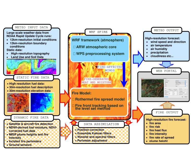
Figure 1: Scheme of wildland fire DDDAS.

The paper is organized as follows. In Sec. 2, we we review some existing approaches to data assimilation in simulations of wildland fires. In Sec. 3 and 4, we briefly formulate the model and the principal idea of creating and replaying artificial fire history from point ignition to a given perimeter, for reference. Sec. 5 considers several methods for the construction of a level set function, needed for the replay, two from our previous work and a new method, which is an extension of the reinitialization equation approach known in level set methods. In Sec. 6, we present a new method how the level set functions constructed for two perimeters can be used to create and replay an artificial fire history between the two perimeters, and a new method that uses the two level set functions for an automatic adjustment of the fire spread rate between the two perimeters. Sec. 7 describes a new moisture model coupled with the fire and atmosphere model, and the possibilities for the assimilation of moisture data. Finally, Sec. 8 is the conclusion.

2 Data assimilation for wildland fires

One way to incorporate data into an executing simulation is by sequential statistical estimation, which takes all available data to date into account, and is known in geosciences as data assimilation. Data assimilation is a standard technique in numerical weather prediction, and the ability to assimilate large amounts of real-time data is behind much of the recent improvement of weather forecast skill [5]. However, data assimilation for wildland fires poses unique challenges, and classical data assimilation methods simply will not work [6, 7, 8]. One of the reasons is that in many other physical systems where standard methods work well, such as pollution transport or atmospheric dynamics, unwanted perturbations tend to dissipate over time; but, in a fire model, once a perturbation ignites an unwanted fire, the fire will keep growing, and after few assimilation cycles, everything burns. Another reason is that a fire as a coherent structure, needs to be moved, started, or extinguished in response to the data, which requires positional, Lagrangean correction; additive corrections of the values of the physical fields are not very useful.

Data assimilation methods by sequential Monte-Carlo methods (SMC), also known as particle filters, were developed in the literature for cell-based fire models [9, 10]. They can handle non-Gaussian distributions, but they are computationally very expensive, because they require very large ensembles to cover a region of the state space by random perturbations. A suitable perturbation algorithm is the key to a successful application. The perturbation methods used in wildland fire modeling range from random modifications of the burn area [9] to genetic algorithms, which evolve the shape of the fire by simulated evolution, where the states with fire regions closer the the data are more likely to survive [11]. While SMC methods with tens of thousands of particles may be feasible for 2D cell models, with relatively small state vectors, they are definitely out of question for a coupled atmosphere-fire model. Methods based on the optimal statistical interpolation and the Kalman filter (KF), such as the ensemble Kalman filter (EnKF), assume that the state distribution is at least approximately Gaussian and they modify the state in response to data [5, p. 180] rather than rely on hitting the right answer with random perturbations. Thus, KF-based mehods require much smaller ensembles that SMC methods, but still in the range of 20-100 members and easily many hundreds [12]. However, because of the fine resolution of the atmospheric model needed over large areas, and the associated need for small time steps, the simulations are computationally very demanding, and such ensembles are still out of question. FFT-based data assimilation methods, which reduce data assimilation to efficient operations with diagonal matrices [13] and can drastically reduce the required ensemble size, from hundreds to often just 5 or 10 members. However, using the Fourier basis is tantamount to the assumption that the state covariance does not vary spatially [14]. Wavelet estimation can combine the effectiveness of spectral methods with an automatic treatment of spatial locality [15]. Wavelet diagonal approximations of the covariance matrix [16] are of particular interest, as they allow efficient evaluation of the EnKF formulas [17].

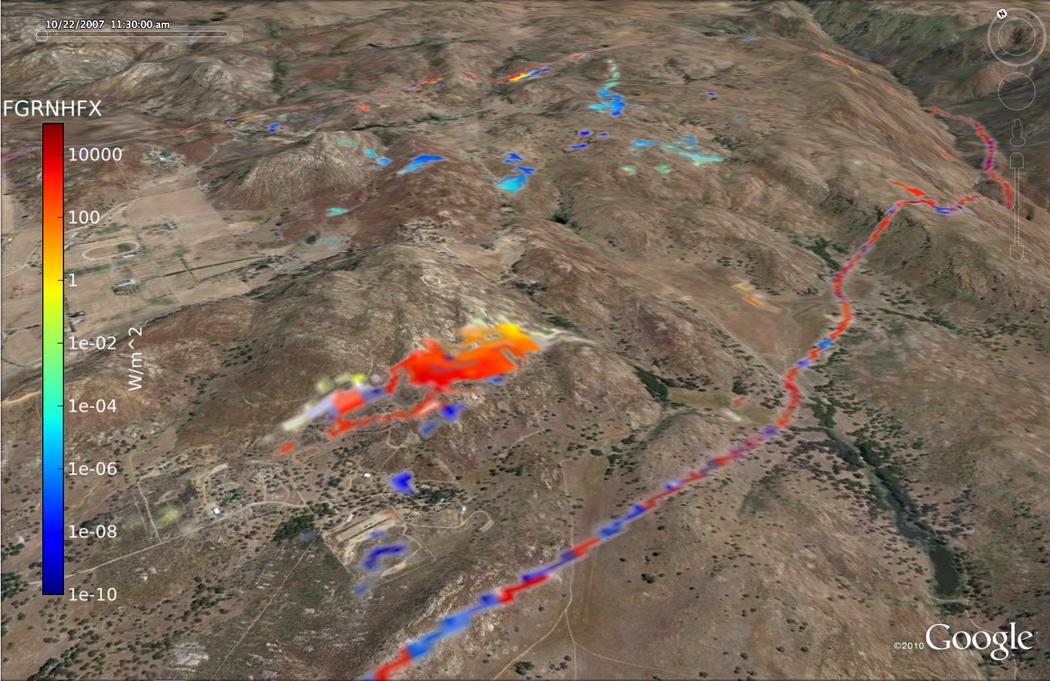
Figure 2: Visualization in Google Earth client, 2007 Witch Fire. False color shows fire heat flux, superimposed on the Earth surface. Patches of slower fuels keep burning behind the fireline. Reproduced from [18].

Position correction methods, such as morphing [6], can overcome the limitations of changing the state of the simulation by additive corrections only. These method extend the state by a new variable containing a deformation field, similarly as in optical flow methods [19] and extraction of the wind field from a sequence of radar images [20]. For other related position correction methods, see, e.g., [21]. Our morphing technique is distinguished by replacing linear combinations of member states, which are at the heart of, e.g., the EnKF, by intermediate states, which interpolate both the magnitude and the position of coherent features, such as fires. Time series of station observations could be handled by considering composite states over several time steps. However, while morphing works successfully for fire models [6, 8], it changes the delicate physical balance of the atmospheric equations and limits the possibility of the treatment of the model as a black box. Even a simple linear transformation to move and reshape the vortex in hurricane forecasting needs rebalancing of the atmospheric variables from conservation equations [22, p. 11].

Therefore, an important problem in data assimilation for a coupled atmosphere-fire model is how to adjust the atmosphere state when the state of the fire model changes in response to data. The heat output of the fire is concentrated in a narrow area with active combustion, therefore the fire forcing on the atmosphere is highly localized. If the fire is just shifted, a position correction alone can be successfull to some extent [6, 8] because the relationship between the changes in the atmosphere and in the fire is captured in the covariance of their deformation fields. However, in general, the covariance does not contain sufficient information and a spin-up is required to develop proper circulation patterns for the changed fire forcing.

3 The coupled atmosphere – fire model

Over time, the wildland fire DDDAS has evolved from a simple convection-reaction-diffusion equation exploratory model to test data assimilation methodologies [23] and the CAWFE model [24, 25], which couples the Clark-Hall atmospheric model with fire spread implemented by tracers (Lagrangean particles), to the currently used Weather Research Forecasting (WRF) mesoscale atmospheric code [26] coupled with a spread model implemented by the level set method [8, 27]. The Clark-Hall model has many favorable properties, such as the ability to handle refinement, but WRF is a supported community model, it can execute in parallel, and has built-in export and import of state, which is essential for data assimilation. Also, WRF supports data formats standard in geosciences. The implementation by the level set method was chosen because the level set function can be manipulated much more easily than tracers. The coupled code is available from the Open Wildland Fire Modeling Environment (OpenWFM) [18] at openwfm.org, which contains also diagnostic and data processing utilities, including visualization in Google Earth (Fig. 2), which we first proposed in [2]. A subset of the SFIRE code was released with WRF as WRF-Fire. The model is capable of running on a cluster faster than real time with atmospheric resolution in tens of m, needed to resolve the atmosphere-fire interaction, for a fire of size over $10$ km [28]. See [8, 27] for futher details and references.

The state variables of the fire model are the level set function, $\Phi$, the time of ignition $T_{\mathrm{i}}$, and the fuel fraction remaining $F$, given by their values on the nodes of the fire model mesh. At a given simulation time $t$, the fire area is represented by the level set function $\Phi$ as the set of all points $\left(x,y\right)$ where $\Phi\left(t,x,y\right)\leq 0$. Since the level set function is interpolated linearly between nodes, this allows a submesh representation of the fire area. In every time step of the simulation, the level set function is advanced by one step of a Runge-Kutta scheme for the level set equation

$$\frac{d\Phi}{dt}=-R\left|\nabla\Phi\right|,$$ (1)

where $R=R\left(t,x,y\right)$ is the fire rate of spread and $\left|\cdot\right|$ is the Euclidean norm. The ignition time $T_{\mathrm{i}}=T_{\mathrm{i}}\left(x,y\right)$ is then computed for all newly ignited nodes, and it satisfies the consistency condition

$$\Phi\left(t,x,y\right)\leq 0\Longleftrightarrow T_{\mathrm{i}}\left(x,y\right)\leq t,$$ (2)

where both inequalities express the condition that the location $\left(x,y\right)$ is burning at the time $t$.

The fire rate of spread $R$ is given by the Rothermel’s formula [29] as a function of the wind speed (at a height dependent on the fuel) and the slope in the direction normal to the fireline. From the level-set representation of the fireline at the time $t$ as $\Phi\left(t,x,y\right)=0$, it follows by an easy calculus that the normal direction is $\nabla\Phi/\left|\nabla\Phi\right|$, where $\left|\cdot\right|$ is the Euclidean norm. Thus,

$$R=R\left(\mathbf{u}\cdot\frac{\nabla\Phi}{\left|\nabla\Phi\right|}\right),$$ (3)

where $\mathbf{u}$ is the wind field.

Once the fuel starts burning, the remaining mass fraction $F=F(t,x,y)$ is approximated by exponential decay,

$$F\left(t,x,y\right)=\left\{\begin{array}[c]{cc}\exp\left(-\frac{t-T_{\mathrm{i}}\left(x,y\right)}{T_{\mathrm{f}}\left(x,y\right)}\right),&t>T_{\mathrm{i}}\left(x,y\right),\\ 1,&t\leq T_{\mathrm{i}}\left(x,y\right),\end{array}\right.$$ (4)

where $T_{\mathrm{f}}$ is the fuel burn time, i.e., the number of seconds for the fuel to burn down to $1/e\approx 0.3689$ of the starting fuel fraction $F=1$. The heat fluxes from the fire to the atmosphere are taken proportional to the fuel burning rate, $\partial F\left(t,x,y\right)/\partial t$. The proportionality constants are fuel coefficients. The heat fluxes from the fire are inserted into the atmospheric model as forcing terms in differential equations of the atmospheric model in a layer above the surface, with exponential decay with altitude. This scheme is required because atmospheric models with explicit timestepping, such as WRF, do not support flux boundary conditions. The sensible heat flux is added to the time derivative of the temperature, while the latent heat flux is added to the derivative of water vapor concentration.

4 Replaying artificial fire history

The SFIRE code as presented in [8, 27] starts from one or more ignition points. The release of the heat from the fire then gradually establishes atmospheric circulation patterns and the fire evolves in an interaction with the atmosphere. There is, however, a practical need to start the simulation from an observed fire perimeter, and to modify the fire perimeter in a running simulation, which presents a particular problem in a coupled model. The atmospheric circulation due to the fire takes time to develop and the heat release from the fire model needs to be gradual, or the model will crash due to excessive vertical wind component.

Therefore, we have proposed creating and replaying an approximate fire history, leading to the desired fire perimeter [30]. Replying the fire history allows for graduate release of the combustion heat and allows the atmospheric circulation patterns due to the fire to develop. The fire history is encoded as an array of ignition times $T_{\mathrm{i}}\left(x,y\right)$, prescribed at all fire mesh nodes. To replay the fire, the numerical scheme for advancing $\Phi$ is suspended, and instead the level set function is set to

$$\Phi\left(t,x,y\right)=T_{\mathrm{i}}\left(x,y\right)-t.$$ (5)

The fuel decay (4) is then computed from $T_{\mathrm{i}}$, and the resulting heat fluxes are inserted into the atmosphere. After the end of the replay period is reached, the numerical scheme of the level set method takes over.

5 Creating a level set function from a given fire perimeter

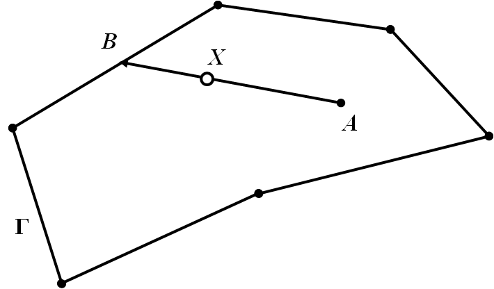
Figure 3: Creating artificial time history by proportions. The ignition times at the ignition point $A$ and the fire perimeter $\Gamma$ are interpolated linearly along the segment between $A$ and a point $B$ on $\Gamma$ to a mesh point $X$.

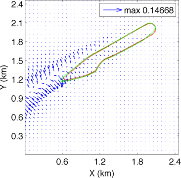
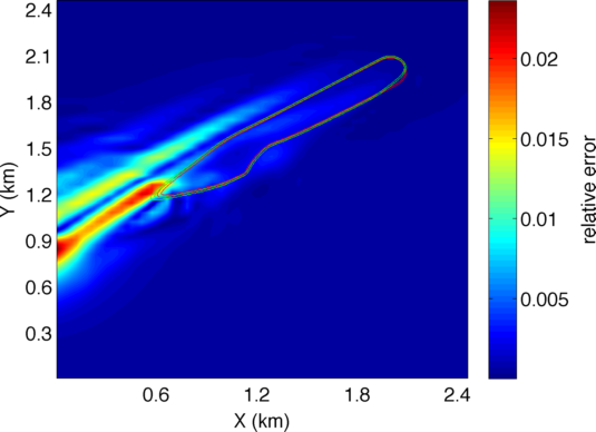
(a) The difference in the horizontal wind vector (m/s).	(b) The relative difference in the wind speed.

Figure 4: The difference in the horizontal wind field at $6.1$m between a simulation propagated naturally from a point and another one advanced artificially. The first simulation was ignited from a point in the northeast corner of the domain, and the fire perimeter was recorded after $40$ minutes. This perimeter and ignition location were used to generate an artificial history for the first $40$ minutes, which was replayed in the second simulation. Both simulations were then allowed to advance another $28$ minutes. Reproduced from [30].

A fire perimeter is considered as a closed curve $\Gamma$, composed of linear segments, and given as a sequence of the coordinates of the endpoints of the segments. In practice, such geospatial data are often provided as a GIS shapefile [31], or encoded in a KML file, e.g., from LANDFIRE.

In [30], we have proposed a simple scheme for creating an artificial fire history to be used in the fire replay scheme (5): given an ignition point and ignition time at that point, approximate ignition times $T_{\mathrm{i}}$ at the mesh points are established by linear interpolation between the ignition point and the perimeter (Fig. 3). This simple method was already shown to be successful in starting the model from the given perimeter in a simple idealized case (Fig. 4), with the error in the wind speed of only few %. Extensions of the artificial history scheme will be needed for domains which are not star-shaped with respect to the ignition point. Running the fire propagation backwards in time to find an ignition point is also a possibility, with an intriguing forensic potential [30].

The ignition times $T_{\mathrm{i}}$ at locations outside of the given fire perimeter are perhaps best thought of as what the ignition times at those locations might be in future as the fire keeps burning.

Constructing a level set function from a perimeter is one of the basic tasks in level set methods. Given a closed curve $\Gamma$, one wishes to construct a function $L=L\left(x,y\right)$, such that

$$L>0\text{ outside of }\Gamma\text{,\quad}L<0\text{ inside of }\Gamma\text{,\quad}L=0\text{ on }\Gamma.$$ (6)

In the application to perimeter ignition, one can then set at a fixed instant $t$,

$$T_{\mathrm{i}}\left(x,y\right)=cL\left(x,y\right)+\left(t-T\right),\quad\Phi\left(t,x,y\right)=L\left(x,y\right)$$

where $c$ is a scaling factor, and proceed with the replay as described in Section 4.

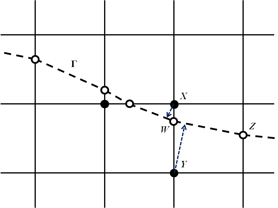
Figure 5: A level set function linear on the line segments connecting the nodes of the fire mesh cannot be defined at the nodes $X$ and $Y$ consistently as the signed distance (7) from the interface $\Gamma$. The distance of the point $X$ from $\Gamma$ does not depend on the location of the point $Z$, while the distance of $Y$ does; yet the values of the level set function at $X$ and $Y$ are linear along the segment $XY$ and so fixed by the ratio of their distances from $W$.

One commonly used level set function is the signed distance from the given closed curve $\Gamma$,

$$L\left(x,y\right)=\pm\operatorname*{dist}\left(\left(x,y\right),\Gamma\right),$$ (7)

where the sign is taken to be negative inside the region limited by $\Gamma$ and positive outside [32], and $\operatorname*{dist}$ stands for the Euclidean distance. Surprisingly, such function cannot be defined consistently once the problem is discretized. Consider a level set function $L$ that is given by its values on the corners of grid cells, interpolated linearly along the grid lines, and $\Gamma$ given by its intersection with the grid lines (Fig. 5). Then, the ratio of the values of $L$ at two neighboring mesh corners on the opposite sides of $\Gamma$ is fixed by the requirement that $L$ is linear between the two corners. In particular, it is not possible in general to define $L$ as the signed distance (7). For example, in Fig. 5, the ratio $L\left(X\right)/L\left(Y\right)$ is fixed and $L\left(X\right)$ does not depend on $Z$, while $L\left(Y\right)$ does.

One possibility is simply define the values of $L$ next to $\Gamma$ by the signed distance, and forget about the exact representation of $\Gamma$ as $L=0.$ Instead, in [33], we have proposed to find the values of $L$ next to $\Gamma$ by least squares. Denoting by $u$ the vector of the values $L$ next to $\Gamma$, it is easy to see that $u$ satisfies a homogeneous system of linear equations of the form $Bu=0$ with at most two nonzeros per rows, and each row corresponding to an edge on the mesh that is intersected by $\Gamma$, as the edge $XY$. We can then find a suitable $u$ minimizing $\left\|u-d\right\|^{2}$ subject to $Bu=0$, where $d$ are the signed distances (7). Once the values of $L$ near $\Gamma$ are found, one can extend $L$ to the whole domain as the distance function by the Fast Marching Method (FMM) [34], or by a simpler and less accurate approximate method suggested in [33].

A better method can be obtained by taking the spread rate into account. The level set function $L$ is a solution of the Hamilton-Jacobi equation

$$R\left|\triangledown L\right|=1,\quad L=0\text{ on }\Gamma.$$

which can be found by solving the reinitialization equation [32, Eq. (7.4)]

$$\frac{\partial L}{\partial t}=\pm\left(1-R\left|\triangledown L\right|\right)$$ (8)

where the sign is taken positive outside of $\Gamma$ and negative inside. Equation (8) is solved by upwinding formulas moving away from $\Gamma$ and starting from the values of $L$ on the other side of $\Gamma$. Alternating the solution process between the outside and the inside of $\Gamma$, the values of $L$ on the two sides of $\Gamma$ “balance out and a steady-state signed distance function is obtained” [32, p. 66].

The situation here is more complicated, because the spread rate $R$ depends on the level set function $L$ following (3). Hence, we freeze $L$ inside $R$ and use successive approximations of the form

$$\frac{\partial L_{k+1}}{\partial t}=\pm\left(1-R\left(\mathbf{u}\cdot\frac{\triangledown L_{k}}{\left|\triangledown L_{k}\right|}\right)\left|\triangledown L_{k+1}\right|\right).$$

6 Data assimilation for the level set fire spread model

Creating a level set function as in [30] and in Sec. 5 allows for starting the coupled model from a given fire perimeter instead of an ignition point. However, a more general approach is needed for data assimilation. Suppose the fire perimeter in the simulation is $\Gamma_{1}$ at time $t_{1}$. Then at time $t_{2}>t_{1}$, the fire evolves to fire perimeter $\Gamma_{2}$. However, data is assimilated, changing the state of the fire model and resulting in a different fire model state with perimeter $\Gamma_{\mathrm{a}}$. First we construct level set functions $L_{1}$, $L_{2}$, and $L_{\mathrm{a}}$ for the perimeters $\Gamma_{1}$, $\Gamma_{2}$, and $\Gamma_{\mathrm{a}}$, respectively, satisfying (6). We assume that all three level set functions are created using the same method. The resulting approximate formulas will be exact in the case of 1D propagation with the level set functions linear and having the same slope. They will be used point-wise as an approximation otherwise. To emphasize the point-wise application, we write out the arguments $\left(x,y\right)$ when present.

6.1 Modifying the fire perimeter dynamically

The state of the atmosphere will no longer match the state of the fire model with the perimeter $\Gamma_{\mathrm{a}}$, and we need to make up the evolution of the atmosphere as the fire progresses from the perimeter $\Gamma_{1}$ to the perimeter $\Gamma_{\mathrm{a}}$. Since $\Gamma_{1}$ is completely contained inside $\Gamma_{\mathrm{a}}$, in the region between $\Gamma_{1}$ and $\Gamma_{\mathrm{a}}$, we have $L_{1}>0$ and $L_{\mathrm{a}}<0$. The function

$$f_{1,a}\left(x,y\right)=\frac{L_{1}\left(x,y\right)}{L_{1}\left(x,y\right)-L_{\mathrm{a}}\left(x,y\right)}$$ (9)

then satisfies

$$f_{1,a}=0\text{ on }\Gamma_{1},\text{\quad}0<f_{1,a}<1\text{ between }\Gamma_{1}\text{ and }\Gamma_{a},\quad f_{1,a}=1\text{ on }\Gamma_{2}\text{.}$$

We can then use the function $f_{1,a}$ to create artificial ignition times by

$$T_{\mathrm{i}}\left(x,y\right)=t_{1}+\frac{L_{1}\left(x,y\right)}{L_{1}\left(x,y\right)-L_{\mathrm{a}}\left(x,y\right)}\left(t_{2}-t_{1}\right)$$

which interpolates between the perimeters $\Gamma_{1}$ and $\Gamma_{\mathrm{a}}$, and replay the fire history to release the heat into the atmosphere gradually, as in Sec. 4.

6.2 Dynamic estimate of fire spread rate

A common source of errors in fire modeling is incorrect spread rate. The level set function construction here can be used to adjust the spread rate as well. Define $f_{1,2}$ similarly to (9),

$$f_{1,2}\left(x,y\right)=\frac{L_{1}\left(x,y\right)}{L_{1}\left(x,y\right)-L_{2}\left(x,y\right)}.$$ (10)

We now use a simple argument of proportions. Assume for the moment 1D fire propagation in one direction and that $f_{1,a}$ and $f_{1,2}$ are linear. Then $\Gamma_{1}$, $\Gamma_{2}$, and $\Gamma_{\mathrm{a}}$ are points on the real line. and the spread rates of the simulated fire and the spread rate after the data assimilation are, respectively,

$$R=\frac{\Gamma_{2}-\Gamma_{1}}{t_{2}-t_{1}},\text{\quad}R_{\mathrm{a}}=\frac{\Gamma_{\mathrm{a}}-\Gamma_{1}}{t_{2}-t_{1}}.$$

However, since $f_{1,2}$ and $f_{1,a}$ are linear,

$$f_{1,2}\left(x\right)=\frac{x-\Gamma_{1}}{\Gamma_{2}-\Gamma_{1}},\text{\quad}f_{1,a}\left(x\right)=\frac{x-\Gamma_{1}}{\Gamma_{a}-\Gamma_{1}},$$

which gives

$$\frac{R_{\mathrm{a}}\left(x\right)}{R\left(x\right)}=\frac{\Gamma_{\mathrm{a}}-\Gamma_{1}}{\Gamma_{2}-\Gamma_{1}}=\frac{f_{1,2}\left(x\right)}{f_{1,a}\left(x\right)},\text{\quad}x\neq\Gamma_{1}.$$ (11)

Thus, using (9) and (10), (11) suggests to modify the given spread rate $R$ at a point $\left(x,y\right)$ to become the spread rate $R_{a}$ after the data assimilation, given by

$$R_{\mathrm{a}}\left(x,y\right)=\frac{L_{1}\left(x,y\right)-L_{a}\left(x,y\right)}{L_{1}\left(x,y\right)-L_{2}\left(x,y\right)}R\left(x,y\right).$$ (12)

7 Moisture model

Fire spread rate depends strongly on the moisture contents of the fuel. In fact, the spread rate drops to zero when the moisture reaches the so-called extinction value. For this reason, we have coupled the fire spread model with a simple fuel moisture model integrated in SFIRE and run independently at every point of the mesh. The temperature and the relative humidity of the air (from the WRF atmosphere model) determine the fuel equilibrium moisture contents $E$ [35], and the actual moisture contents $m=m\left(t\right)$ is then modeled by the standard time-lag equation

$$\frac{dm}{dt}=\frac{E-m}{T_{\mathrm{d}}},$$ (13)

where $T_{\mathrm{d}}$ is the drying lag time. We use the standard model with the fuel consisting of components with $1$, $10$, and $100$ hour lag time, with the proportions given by the fuel category [36], and the moisture is tracked in each component separately. During rain, the equilibrium moisture $E$ is replaced by the saturation moisture contents $S$, and the equation is modified to achieve the rain-wetting lag time $T_{\mathrm{r}}$ only asymptotically for heavy rain,

$$\frac{dm}{dt}=\frac{S-m}{T_{\mathrm{r}}}\left(1-\exp\left(-\frac{r-r_{0}}{r_{\mathrm{s}}}\right)\right),\text{ if }r>r_{0},$$ (14)

where $r$ is the rain intensity, $r_{0}$ is the threshold rain intensity below which no perceptible wetting occurs, and $r_{\mathrm{s}}$ is the saturation rain intensity, at which $1-1/e\approx 63\%$ of the maximal rain-wetting rate is achieved. The coefficients can be calibrated to achieve a similar behavior as accepted empirical models [37, 38]. See [39, 40] for other, much more sophisticated models. If moisture measurements are available, they can be ingested in the model (13, 14) by a fast and cheap Kalman filter in one variable, run at each point independently.

8 Conclusion

We have presented new techniques to assimilate the perimeter data at two different times into a coupled atmosphere-fire model, a new method to estimate the adjustment of the model spread rate between the perimeters towards the data, and a new coupling of the atmosphere-fire model with a third model, a simple time-lag model of fuel moisture. Implementation of the data assimilation is in progress. The moisture model is currently included in the code download and will be treated in more detail elsewhere.

References

References

- [1] J. Mandel, M. Chen, L. P. Franca, C. Johns, A. Puhalskii, J. L. Coen, C. C. Douglas, R. Kremens, A. Vodacek, W. Zhao, A note on dynamic data driven wildfire modeling, in: M. Bubak, G. D. van Albada, P. M. A. Sloot, J. J. Dongarra (Eds.), Computational Science – ICCS 2004, Vol. 3038 of Lecture Notes in Computer Science, Springer, 2004, pp. 725–731. doi:10.1007/b97989.
- [2] C. C. Douglas, J. D. Beezley, J. Coen, D. Li, W. Li, A. K. Mandel, J. Mandel, G. Qin, A. Vodacek, Demonstrating the validity of a wildfire DDDAS, in: V. N. Alexandrov, D. G. van Albada, P. M. A. Sloot, J. Dongarra (Eds.), Computational Science – ICCS 2006, Vol. 3993 of Lecture Notes in Computer Science, Springer, 2006, pp. 522–529. doi:10.1007/11758532_69.
- [3] J. Beezley, S. Chakraborty, J. Coen, C. Douglas, J. Mandel, A. Vodacek, Z. Wang, Real-time data driven wildland fire modeling, in: M. Bubak, G. van Albada, J. Dongarra, P. Sloot (Eds.), Computational Science – ICCS 2008, Vol. 5103 of Lecture Notes in Computer Science, Springer, 2008, pp. 46–53. doi:10.1007/978-3-540-69389-5_7.
- [4] F. Darema, Dynamic data driven applications systems: A new paradigm for application simulations and measurements, in: M. Bubak, G. van Albada, P. Sloot, J. Dongarra (Eds.), Computational Science – ICCS 2004, Vol. 3038 of Lecture Notes in Computer Science, Springer, 2004, pp. 662–669. doi:10.1007/978-3-540-24688-6_86.
- [5] E. Kalnay, Atmospheric Modeling, Data Assimilation and Predictability, Cambridge University Press, 2003.
- [6] J. D. Beezley, J. Mandel, Morphing ensemble Kalman filters, Tellus 60A (2008) 131–140. doi:10.1111/j.1600-0870.2007.00275.x.
- [7] C. J. Johns, J. Mandel, A two-stage ensemble Kalman filter for smooth data assimilation, Environmental and Ecological Statistics 15 (2008) 101–110. doi:10.1007/s10651-007-0033-0.
- [8] J. Mandel, J. D. Beezley, J. L. Coen, M. Kim, Data assimilation for wildland fires: Ensemble Kalman filters in coupled atmosphere-surface models, IEEE Control Systems Magazine 29 (3) (2009) 47–65. doi:10.1109/MCS.2009.932224.
- [9] G. Bianchini, A. Cortés, T. Margalef, E. Luque, Improved prediction methods for wildfires using high performance computing: A comparison, in: V. Alexandrov, G. van Albada, P. Sloot, J. Dongarra (Eds.), Computational Science – ICCS 2006, Vol. 3991 of Lecture Notes in Computer Science, Springer, 2006, pp. 539–546. doi:10.1007/11758501_73.
- [10] F. Gu, X. Hu, Towards applications of particle filters in wildfire spread simulation, in: WSC ’08: Proceedings of the 40th Conference on Winter Simulation, IEEE, 2008, pp. 2852–2860. doi:10.1109/WSC.2008.4736406.
- [11] M. Denham, A. Cortés, T. Margalef, Computational steering strategy to calibrate input variables in a dynamic data driven genetic algorithm for forest fire spread prediction, in: Computational Science–ICCS 2009, Vol. 5545 of Lecture Notes in Computer Science, Springer, 2009, pp. 479–488. doi:10.1007/978-3-642-01973-9_54.
- [12] G. Evensen, Data Assimilation: The Ensemble Kalman Filter, 2nd Edition, Springer, 2009. doi:10.1007/978-3-642-03711-5.
- [13] J. Mandel, J. D. Beezley, V. Y. Kondratenko, Fast Fourier transform ensemble Kalman filter with application to a coupled atmosphere-wildland fire model, in: A. M. Gil-Lafuente, J. M. Merigo (Eds.), Computational Intelligence in Business and Economics, Proceedings of MS’10, World Scientific, 2010, pp. 777–784, available as arXiv:1001.1588. doi:10.1142/9789814324441_0089.
- [14] L. Berre, Estimation of synoptic and mesoscale forecast error covariances in a limited-area model, Monthly Weather Review 128 (3) (2000) 644–667. doi:10.1175/1520-0493(2000)128<0644:EOSAMF>2.0.CO;2.
- [15] A. Deckmyn, L. Berre, A wavelet approach to representing background error covariances in a limited-area model, Monthly Weather Review 133 (5) (2005) 1279–1294. doi:10.1175/MWR2929.1.
- [16] O. Pannekoucke, Heterogeneous correlation modeling based on the wavelet diagonal assumption and on the diffusion operator, Monthly Weather Review 137 (9) (2009) 2995–3012. doi:10.1175/2009MWR2783.1.
- [17] J. D. Beezley, J. Mandel, L. Cobb, Wavelet ensemble Kalman filters, in: Proceedings of IEEE IDAACS’2011, Prague, September 2011, Vol. 2, IEEE, 2011, pp. 514–518. doi:10.1109/IDAACS.2011.6072819.
- [18] J. Mandel, J. D. Beezley, A. K. Kochanski, V. Y. Kondratenko, L. Zhang, E. Anderson, J. Daniels II, C. T. Silva, C. R. Johnson, A wildland fire modeling and visualization environment, Paper 6.4, Ninth Symposium on Fire and Forest Meteorology, Palm Springs, October 2011, available at http://ams.confex.com/ams/9FIRE/webprogram/Paper192277.html, retrieved December 2011 (2011).
- [19] C. Marzban, S. Sandgathe, H. Lyons, N. Lederer, Three spatial verification techniques: Cluster analysis, variogram, and optical flow, Weather and Forecasting 24 (6) (2009) 1457–1471. doi:{10.1175/2009WAF2222261.1}.
- [20] S. Laroche, I. Zawadzki, A variational analysis method for retrieval of three-dimensional wind field from single-Doppler radar data, Journal of the Atmospheric Sciences 51 (18) (1994) 2664–2682. doi:10.1175/1520-0469(1994)051<2664:AVAMFR>2.0.CO;2.
- [21] S. Ravela, K. A. Emanuel, D. McLaughlin, Data assimilation by field alignment, Physica D 230 (2007) 127–145. doi:10.1016/j.physd.2006.09.035.
- [22] S. Gopalakrishnan, Q. Liu, T. Marchok, D. Sheinin, N. Surgi, R. Tuleya, R. Yablonsky, X. Zhang, Hurricane Weather and Research and Forecasting (HWRF) model scientific documentation, NOAA, http://www.dtcenter.org/HurrWRF/users/docs/scientific_documents/HWRF_final_2-2_cm.pdf, retrieved October 2011 (2010).
- [23] J. Mandel, L. S. Bennethum, J. D. Beezley, J. L. Coen, C. C. Douglas, M. Kim, A. Vodacek, A wildland fire model with data assimilation, Mathematics and Computers in Simulation 79 (2008) 584–606. doi:10.1016/j.matcom.2008.03.015.
- [24] T. L. Clark, M. A. Jenkins, J. Coen, D. Packham, A coupled atmospheric-fire model: Convective feedback on fire line dynamics, Journal of Applied Meteorolgy 35 (1996) 875–901. doi:10.1175/1520-0450(1996)035<0875:ACAMCF>2.0.CO;2.
- [25] T. L. Clark, J. Coen, D. Latham, Description of a coupled atmosphere-fire model, International Journal of Wildland Fire 13 (2004) 49–64. doi:10.1071/WF03043.
- [26] W. C. Skamarock, J. B. Klemp, J. Dudhia, D. O. Gill, D. M. Barker, M. G. Duda, X.-Y. Huang, W. Wang, J. G. Powers, A description of the Advanced Research WRF version 3, NCAR Technical Note 475, http://www.mmm.ucar.edu/wrf/users/docs/arw_v3.pdf, retrieved December 2011 (2008).
- [27] J. Mandel, J. D. Beezley, A. K. Kochanski, Coupled atmosphere-wildland fire modeling with WRF 3.3 and SFIRE 2011, Geoscientific Model Development 4 (2011) 591–610. doi:10.5194/gmd-4-591-2011.
- [28] G. Jordanov, J. D. Beezley, N. Dobrinkova, A. K. Kochanski, J. Mandel, B. Sousedík, Simulation of the 2009 Harmanli fire (Bulgaria), in: I. Lirkov, S. Margenov, J. Wanśiewski (Eds.), 8th International Conference on Large-Scale Scientific Computations, Sozopol, Bulgaria, June 6-10, 2011, Vol. 7116 of Lecture Notes in Computer Science, Springer, 2012, pp. 291–298, also available as arXiv:1106.4736.
- [29] R. C. Rothermel, A mathematical model for predicting fire spread in wildland fires, USDA Forest Service Research Paper INT-115, http://www.treesearch.fs.fed.us/pubs/32533 (1972).
- [30] V. Y. Kondratenko, J. D. Beezley, A. K. Kochanski, J. Mandel, Ignition from a fire perimeter in a WRF wildland fire model, Paper 9.6, 12th WRF Users’ Workshop, National Center for Atmospheric Research, June 20-24, 2011, http://www.mmm.ucar.edu/wrf/users/workshops/WS2011/WorkshopPapers.php, retrieved August 2011 (2011).
- [31] ESRI shapefile technical description, An ESRI White Paper, Environmental Systems Research Institute, Inc., http://www.esri.com/library/whitepapers/pdfs/shapefile.pdf, retrieved January 2012 (1998).
- [32] S. Osher, R. Fedkiw, Level Set Methods and Dynamic Implicit Surfaces, Springer, New York, 2003.
- [33] J. Mandel, V. Kulkarni, Construction of a level function for fireline data assimilation, CCM Technical Report 234, University of Colorado at Denver, http://ccm.ucdenver.edu/reports/rep234.pdf (June 2006).
- [34] J. A. Sethian, Level set methods and fast marching methods, 2nd Edition, Vol. 3 of Cambridge Monographs on Applied and Computational Mathematics, Cambridge University Press, Cambridge, 1999.
- [35] N. R. Viney, A review of fine fuel moisture modelling, International Journal of Wildland Fire 1 (4) (1991) 215–234. doi:10.1071/WF9910215.
- [36] J. H. Scott, R. E. Burgan, Standard fire behavior fuel models: A comprehensive set for use with Rothermel’s surface fire spread model, Gen. Tech. Rep. RMRS-GTR-153. Fort Collins, CO: U.S. Department of Agriculture, Forest Service, Rocky Mountain Research Station, http://www.fs.fed.us/rm/pubs/rmrs_gtr153.html (2005).
- [37] M. A. Fosberg, J. E. Deeming, Derivation of the 1- and 10-hour timelag fuel moisture calculations for fire-danger rating, U.S. Forest Service Research Note RM-207, http://hdl.handle.net/2027/umn.31951d02995763p (1971).
- [38] C. E. Van Wagner, T. L. Pickett, Equations and FORTRAN program for the Canadian forest fire weather index system, Canadian Forestry Service, Forestry Technical Report 33 (1985).
- [39] R. M. Nelson Jr., Prediction of diurnal change in 10-h fuel stick moisture content, Canadian Journal of Forest Research 30 (7) (2000) 1071–1087. doi:10.1139/x00-032.
- [40] D. R. Weise, F. M. Fujioka, R. M. Nelson Jr., A comparison of three models of 1-h time lag fuel moisture in Hawaii, Agricultural and Forest Meteorology 133 (2005) 28–39. doi:10.1016/j.agrformet.2005.03.012.