A network-based dynamical ranking system for competitive sports

Abstract

From the viewpoint of networks, a ranking system for players or teams in sports is equivalent to a centrality measure for sports networks, whereby a directed link represents the result of a single game. Previously proposed network-based ranking systems are derived from static networks, i.e., aggregation of the results of games over time. However, the score of a player (or team) fluctuates over time. Defeating a renowned player in the peak performance is intuitively more rewarding than defeating the same player in other periods. To account for this factor, we propose a dynamic variant of such a network-based ranking system and apply it to professional men’s tennis data. We derive a set of linear online update equations for the score of each player. The proposed ranking system predicts the outcome of the future games with a higher accuracy than the static counterparts.

1 Introduction

Ranking of individual players or teams in sports, both professional and amateur, is a tool for entertaining fans and developing sports business. Depending on the type of sports, different ranking systems are in use [1]. A challenge in sports ranking is that it is often impossible for all the pairs of players or teams (we refer only to players in the following. However, the discussion also applies to team sports) to fight against each other. This is the case for most individual sports and some team sports in which a league contains many teams, such as American college football and soccer at an international level. Then, the set of opponents depends on players such that ranking players by simply counting the number of wins and losses is inappropriate.

In this situation, several ranking systems on the basis of networks have been proposed. A player is regarded to be a node in a network, and a directed link from the winning player to the losing player (or the converse) represents the result of a single game. Once the directed network of players is generated, ranking the players is equivalent to defining a centrality measure for the network. A crux in constructing a network-based ranking system is to let a player that beats a strong player gain a high score. Examples of network-based ranking systems include those derived from the Laplacian matrix of the network [2, 3, 4, 5], the PageRank [6], a random walk that is different from those implied by the Laplacian or PageRank [7], a combination of node degree and global structure of networks [8], and the so-called win-lose score [9].

Previous network-based ranking systems do not account for fluctuations of rankings. In fact, a player, even a history making strong player, referred to as $X$, is often weak in the beginning of the career. Player $X$ may also be weak past the most brilliant period in the $X$’s career, suggestive of the retirement in a near future. For other players, it is more rewarding to beat $X$ when $X$ is in the peak performance than when $X$ is novice, near the retirement, or in the slump. It may be preferable to take into account the dynamics of players’ strengths for defining a ranking system. In the present study, we extend the win-lose score, a network-based ranking system proposed by Park and Newman [9] to the dynamical case. Then, we apply the proposed ranking system to the professional men’s tennis data.

In broader contexts, the current study is related to at least two other lineages of researches. First, a dynamic network-based ranking implies that we exploit the temporal information about the data, i.e., the times when games are played. Therefore, such a ranking system is equivalent to a dynamic centrality measure for temporal networks, in which sequences of pairwise interaction events with time stamps are building units of the network [10]. Although some centrality measures specialized in temporal networks have been proposed [11, 12, 13], they are not for ranking purposes. In addition, they are constant valued centrality measures for dynamic (i.e., temporal) data of pairwise interaction. In the context of temporal networks, we propose a dynamically changing centrality measure for temporal networks.

Second, statistical approaches to sports ranking have a much longer history than network approaches. Representative statistical ranking systems include the Elo system [14] and the Bradley-Terry model (see [15] for a review). Variants of these models have been used to construct dynamic ranking systems. Empirical Bayes framework naturally fits this problem [16, 17, 18, 19, 20, 21]. Because the Bayesian estimators cannot be obtained analytically, or even numerically owing to the computational cost, in these models, techniques for obtaining Bayes estimators such as the Gaussian assumption of the posterior distribution [18, 21], approximate message passing [21], and Kalman filter [17, 18, 19], have been employed. In a non-Bayesian statistical ranking system, the pseudo likelihood, which is defined such that the contribution of the past game results to the current pseudo likelihood decays exponentially in time, is numerically maximized [22].

In general, the parameter set of a statistical ranking system that accounts for dynamics of players’ strengths is composed of dynamically changing strength parameters for all the players and perhaps other auxiliary parameters. Therefore, the number of parameters to be statistically estimated may be large relative to the amount of data. In other words, the instantaneous ranks of players have to be estimated before the players play sufficiently many games with others under fixed strengths. Even under a Bayesian framework with which updating of the parameter values is naturally implemented, it may be difficult to reliably estimate dynamic ranks of players due to relative paucity of data. In addition, in sports played by individuals, such as tennis, it frequently occurs that new players begin and old and underperforming players leave. This factor also increases the number of parameters of a ranking system. In contrast, ours and other network-based ranking systems, both static and dynamic ones, are not founded on statistical methods. Network-based ranking systems can be also simpler and more transparent than statistical counterparts.

Results

Dynamic win-lose score

We extend the win-lose score [9] (see Methods) to account for the fact that the strengths of players fluctuate over time. In the following, we refer to the win-lose score as the original win-lose score and the extended one as the dynamic win-lose score.

The original win-lose score overestimates the real strength of a player $i$ when $i$ defeated an opponent $j$ that is now strong and was weak at the time of the match between $i$ and $j$. Because $j$ defeats many strong opponents afterward, $i$ unjustly receives many indirect wins through $j$. The same logic also applies to other network-based static ranking systems [2, 3, 4, 5, 6, 7, 8].

To remedy this feature, we pose two assumptions. First, we assume that the increment of the win score of player $i$ through the $i$’s winning against player $j$ depends on the $j$’s win score at that moment. It does not explicitly depend on the $j$’s score in the past or future. The same holds true for the lose score. Second, we assume that each player’s win and lose scores decay exponentially in time. This assumption is also employed in a Bayesian dynamic ranking system [22].

Let $A_{t_{n}}$ be the win-lose matrix for the game that occurs at time $t_{n}$ ($1\leq n\leq n_{\max}$). In the analysis of the tennis data carried out in the following, the resolution of $t_{n}$ is equal to one day. Therefore, players’ scores change even within a single tournament. If player $j$ wins against player $i$ at time $t_{n}$, we set the $(i,j)$ element of the matrix $A_{t_{n}}$ to be 1. All the other elements of $A_{t_{n}}$ are set to 0. We define the dynamic win score at time $t_{n}$ in vector form, denoted by $\bm{w}_{t_{n}}$, as follows:

$$W_{t_{n}}= A_{t_{n}}+e^{-\beta(t_{n}-t_{n-1})}\sum_{m_{n}\in\{0,1\}}\alpha^{m_{n}}A_{t_{n-1}}A_{t_{n}}^{m_{n}}$$

$$+e^{-\beta(t_{n}-t_{n-2})}\sum_{m_{n-1},m_{n}\in\{0,1\}}\alpha^{m_{n-1}+m_{n}}A_{t_{n-2}}A_{t_{n-1}}^{m_{n-1}}A_{t_{n}}^{m_{n}}$$

$$+\cdots+e^{-\beta(t_{n}-t_{1})}\sum_{m_{2},\ldots,m_{n}\in\{0,1\}}\alpha^{\sum_{i=2}^{n}m_{i}}A_{t_{1}}A_{t_{2}}^{m_{2}}\cdots A_{t_{n}}^{m_{n}}$$ (1)

and

$$\bm{w}_{t_{n}}=W_{t_{n}}^{\top}\bm{1},$$ (2)

where $\alpha$ is the weight of the indirect win, which is the same as the case of the original win-lose score (Methods), and $\beta\geq 0$ represents the decay rate of the score.

The first term on the right-hand side of Eq. (1) (i.e., $A_{t_{n}}$) represents the effect of the direct win at time $t_{n}$. The second term consists of two contributions. For $m_{n}=0$, the quantity inside the summation represents the direct win at time $t_{n-1}$, which results in weight $e^{-\beta(t_{n}-t_{n-1})}$. For $m_{n}=1$, the quantity represents the indirect win. The ($i$, $j$) element of $A_{t_{n-1}}A_{t_{n}}$ is positive if and only if player $j$ wins against a player $k$ at time $t_{n}$ and $k$ wins against $i$ at time $t_{n-1}$. Player $i$ gains score $e^{-\beta(t_{n}-t_{n-1})}\alpha$ out of this situation. For both cases $m_{n}=0$ and $m_{n}=1$, the $j$th column of the second term accounts for the effect of the $j$’s win at time $t_{n-1}$. The third term covers four cases. For $m_{n-1}=m_{n}=0$, the quantity inside the summation represents the direct win at $t_{n-2}$, resulting in weight $e^{-\beta(t_{n}-t_{n-2})}$. For $m_{n-1}=0$ and $m_{n}=1$, the quantity represents the indirect win based on the games at $t_{n-2}$ and $t_{n}$, resulting in weight $e^{-\beta(t_{n}-t_{n-2})}\alpha$. For $m_{n-1}=1$ and $m_{n}=0$, the quantity represents the indirect win based on the games at $t_{n-2}$ and $t_{n-1}$, resulting in weight $e^{-\beta(t_{n}-t_{n-2})}\alpha$. For $m_{n-1}=m_{n}=1$, the quantity represents the indirect win based on the games at $t_{n-2}$, $t_{n-1}$, and $t_{n}$, resulting in weight $e^{-\beta(t_{n}-t_{n-2})}\alpha^{2}$. In either of the four cases, the $j$th column of the third term accounts for the effect of the $j$’s win at time $t_{n-2}$.

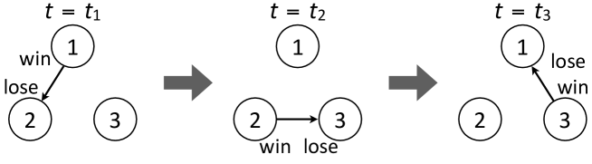
Figure 1: Example time series of games with $N=3$.

To see the difference between the original and dynamic win scores, consider the exemplary data with $N=3$ players shown in Fig. 1. The original win-lose scores calculated from the aggregation of the data up to time $t_{n}$ ($n=1,2$, and 3), denoted by $w_{t_{n}}(i)$ for player $i$, are given by

$$\begin{cases}w_{t_{1}}(1)=1,\\ w_{t_{1}}(2)=0,\\ w_{t_{1}}(3)=0,\end{cases}\begin{cases}w_{t_{2}}(1)=1+\alpha,\\ w_{t_{2}}(2)=1,\\ w_{t_{2}}(3)=0,\end{cases}\begin{cases}w_{t_{3}}(1)=1+\alpha+\alpha^{2}+\cdots,\\ w_{t_{3}}(2)=1+\alpha+\alpha^{2}+\cdots,\\ w_{t_{3}}(3)=1+\alpha+\alpha^{2}+\cdots.\end{cases}$$ (3)

The scores of the three players are the same at $t=t_{3}$ because the aggregated network is symmetric (i.e., directed cycle) if we discard the information about the time.

The dynamic win-lose scores for the same data are given by

$$\begin{cases}w_{t_{1}}(1)=1,\\ w_{t_{1}}(2)=0,\\ w_{t_{1}}(3)=0,\end{cases}\begin{cases}w_{t_{2}}(1)=e^{-\beta(t_{2}-t_{1})},\\ w_{t_{2}}(2)=1,\\ w_{t_{2}}(3)=0,\end{cases}\begin{cases}w_{t_{3}}(1)=e^{-\beta(t_{3}-t_{1})},\\ w_{t_{3}}(2)=e^{-\beta(t_{3}-t_{2})},\\ w_{t_{3}}(3)=1+\alpha e^{-\beta(t_{3}-t_{1})}.\end{cases}$$ (4)

The score of player 1 at $t_{2}$ (i.e., $w_{t_{2}}(1)$) differs from the original win-lose score in two aspects. First, it is discounted by factor $e^{-\beta(t_{2}-t_{1})}$. Second, the value of $w_{t_{2}}(1)$ indicates that player 1 does not gain an indirect win. This is because it is after player 1 defeated player 2 that player 2 defeats player 3. In contrast, player 3 gains an indirect win at $t=t_{3}$ because player 3 defeats player 1, which defeated player 2 before (i.e., at $t=t_{1}$). It should be noted that the win scores of the three players are different at $t=t_{3}$ although the aggregated network is symmetric.

Equation (1) leads to

$$W_{t_{n}}= A_{t_{n}}+e^{-\beta(t_{n}-t_{n-1})}\left[A_{t_{n-1}}+e^{-\beta(t_{n-1}-t_{n-2})}\sum_{m_{n-1}\in\{0,1\}}\alpha^{m_{n-1}}A_{t_{n-2}}A_{t_{n-1}}^{m_{n-1}}\right.$$

$$+\cdots$$

$$\left.+e^{-\beta(t_{n-1}-t_{1})}\sum_{m_{2},\ldots,m_{n-1}\in\{0,1\}}\alpha^{\sum_{i=2}^{n-1}m_{i}}A_{t_{1}}A_{t_{2}}^{m_{2}}\cdots A_{t_{n-1}}^{m_{n-1}}\right]\sum_{m_{n}\in\{0,1\}}\alpha^{m_{n}}A_{t_{n}}^{m_{n}}$$

$$= A_{t_{n}}+e^{-\beta(t_{n}-t_{n-1})}W_{t_{n-1}}(I+\alpha A_{t_{n}}).$$ (5)

Therefore, by combining Eqs. (2) and (5), we obtain the update equation for the dynamic win score as follows:

$$\bm{w}_{t_{n}}=\begin{cases}A_{t_{1}}^{\top}\bm{1}&(n=1),\\ A_{t_{n}}^{\top}\bm{1}+e^{-\beta(t_{n}-t_{n-1})}(I+\alpha A_{t_{n}}^{\top})\bm{w}_{t_{n-1}}&(n>1).\end{cases}$$ (6)

The dynamic lose score at time $t_{n}$ is denoted in vector form by $\bm{\ell}_{t_{n}}$. We obtain the update equation for $\bm{\ell}_{t_{n}}$ by replacing $A_{t_{n}}$ in Eq. (6) by $A_{t_{n}}^{\top}$ as follows:

$$\bm{\ell}_{t_{n}}=\begin{cases}A_{t_{1}}\bm{1}&(n=1),\\ A_{t_{n}}\bm{1}+e^{-\beta(t_{n}-t_{n-1})}(I+\alpha A_{t_{n}})\bm{\ell}_{t_{n-1}}&(n>1).\end{cases}$$ (7)

Finally, the dynamic win-lose score at time $t_{n}$, denoted by $\bm{s}_{t_{n}}$, is given by

$$\bm{s}_{t_{n}}=\bm{w}_{t_{n}}-\bm{\ell}_{t_{n}}.$$ (8)

It should be noted that we do not treat retired players in special ways. Players’ scores exponentially decay after retirement.

Predictability

We apply the dynamic win-lose score to results of professional men’s tennis. The nature of the data is described in Methods.

In this section, we predict the outcomes of future games based on different ranking systems. The frequency of violations, whereby a lower ranked player wins against a higher ranked player in a game, quantifies the degree of predictability [24, 25]. In other literature, the retrodictive version of the frequency of violations is also used for assessing the performance of ranking systems [24, 26, 27, 28].

We compare the predictability of the dynamic win-lose score, the original win-lose score [9], and the prestige score (Methods). The prestige score, proposed by Radicchi and applied to professional men’s tennis data [6], is a static ranking system and is a version of the PageRank originally proposed for ranking webpages [29]. We also implement a dynamic version of the prestige score (Methods) and compare its performance of prediction with that of the dynamic win-lose score.

We define the frequency of violations as follows. We calculate the score of each player at $t_{n}$ ($1\leq n\leq n_{\max}-1$) on the basis of the results up to $t_{n}$. For the original win-lose score and prestige score, we aggregate the directed links from $t=t_{1}$ to $t=t_{n}$ to construct a static network and calculate the players’ scores. If the result of each game at $t_{n+1}$ is inconsistent with the calculated ranking, we regard that a violation occurs. If the two players involved in the game at $t_{n+1}$ have exactly the same score, we regard that a tie occurs irrespective of the result of the game. We define the prediction accuracy at the $N_{\rm gp}$th game as the fraction of correct prediction when the results of the games from $t=t_{2}$ through the $N_{\rm gp}$th game are predicted. The prediction accuracy is given by $\left(N_{\rm gp}^{\prime}-e-v\right)/\left(N_{\rm gp}^{\prime}-e\right)$, where $N_{\rm gp}^{\prime}(<N_{\rm gp})$ is the number of predicted games, $v$ is the number of violations, and $e$ is the number of ties.

For the prestige score and its dynamic variant, we exclude the games in which either player plays for the first time because the score is not defined for the players that have never played. In this case, we increment $e$ by one.

The original and dynamic win-lose scores can be negative valued. Equations (2) and (12) guarantee that the initial score is equal to zero for all the players for the dynamic and original win-lose scores, respectively. Furthermore, any player has a zero win-lose score when the player fights a game for the first time. Even though we do not treat such a game as tie unless both players involved in the game have zero scores, treating it as tie little affects the following results.

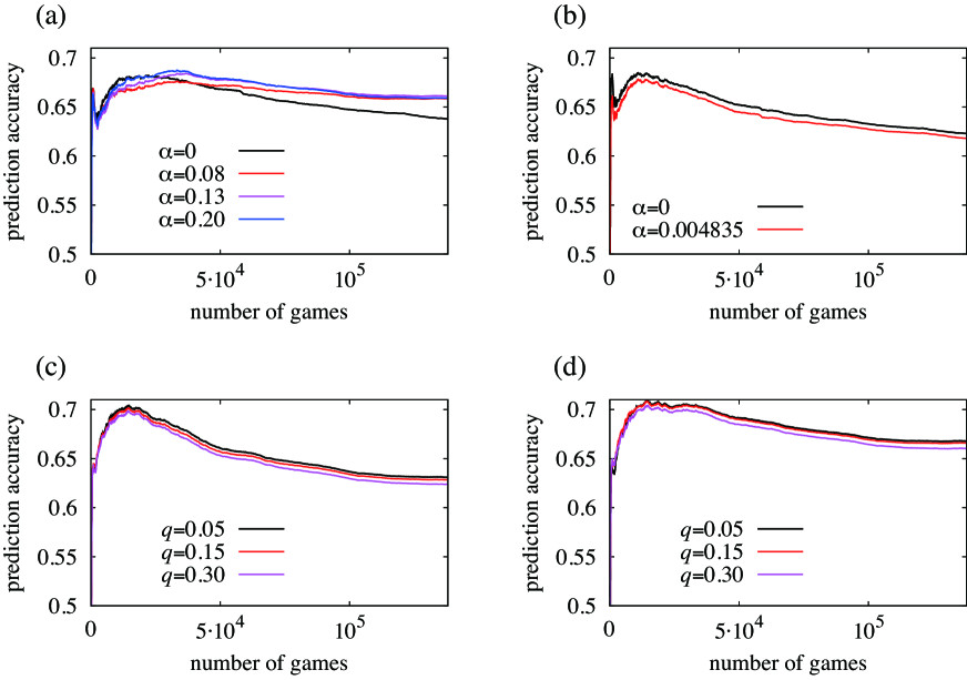
Figure 2: Performance of prediction for the four ranking systems. (a) Dynamic win-lose score with $\beta=1/365$ and different $\alpha$ values. (b) Original win-lose score with $\alpha=0$ and 0.004835. (c) Prestige score with $q=0.05$, 0.15, and 0.3. (d) Dynamic variant of the prestige score with $q=0.05$, 0.15, and 0.3.

The prediction accuracy for the dynamic win-lose score, original win-lose score, prestige score, and dynamic prestige score are shown in Figs. 2(a), 2(b), 2(c), and 2(d), respectively, for various parameter values.

Figure 2(a) indicates that the prediction accuracy for the dynamic win-lose score is the largest for $\alpha=0.13$ except when the number of games (i.e., $N_{\rm gp}$) is small. The accuracy is insensitive to $\alpha$ when $0.08\leq\alpha\leq 0.2$. In this range of $\alpha$, we confirmed by additional numerical simulations that the results for $\beta=1/365$ and those for $\beta=0$ are indistinguishable. Therefore, we conclude that the performance of prediction has some robustness with respect to $\alpha$ and $\beta$. We also confirmed that the accuracy monotonically increases between $\alpha\approx 0.03$ and $\alpha\approx 0.13$. However, for an unknown reason, the accuracy with $\alpha\approx 0.03$ is smaller than that with $\alpha=0$ (results not shown).

Figure 2(b) indicates that the prediction accuracy for the original win-lose score is larger for $\alpha=0$ than $\alpha=0.004835$. The latter $\alpha$ value is very close to the upper limit calculated from the largest eigenvalue of $A$ (see subsection “Parameter values” in Methods). We also found that the prediction accuracy monotonically decreases with $\alpha$. Nevertheless, except for small $N_{\rm gp}$, the accuracy with $\alpha=0$ is lower than that for the dynamic win-lose score with $\alpha=0$ and $0.08\leq\alpha\leq 0.2$ (Fig. 2(a)).

Figure 2(c) indicates that the prediction by the prestige score is better for a smaller value of $q$ (see Methods for the meaning of $q$). We confirmed that this is the case for other values of $q$ and that the results with $q\leq 0.05$ little differ from those with $q=0.05$. Except for small $N_{\rm gp}$, the prediction accuracy with $q=0.05$ is lower than that for the dynamic win-lose score with $0.08\leq\alpha\leq 0.2$ (Fig. 2(a)).

Figure 2(d) indicates that the prediction by the dynamic variant of the prestige score is more accurate than that by the dynamic win-lose score, in particular for small $N_{\rm gp}$. Similar to the case of the original prestige score, the prediction accuracy decreases with $q$.

The findings obtained from Fig. 2 are summarized as follows. When $\alpha$ is between $\approx 0.08$ and $\approx 0.2$ and $\beta$ is between 0 and $1/365$, the dynamic win-lose score outperforms the original win-lose score and the prestige score in the prediction accuracy. For example, at the end of the data, the accuracy is equal to 0.659, 0.661, 0.661, and 0.659 for the dynamic win-lose score with ($\alpha$, $\beta$) $=$ (0.08, $1/365$), (0.1, $1/365$), (0.13, $1/365$), and (0.2, $1/365$), respectively, while it is equal to 0.623 for the original win-lose score with $\alpha=0$ and 0.631 for the prestige score with $q=0.05$. However, the accuracy for the dynamic variant of the prestige score with $q=0.05$ (i.e., 0.668) is slightly larger than the largest value obtained by the dynamic win-lose score.

We also compare the prediction accuracy for the dynamic win-lose score with that for the official Association of Tennis Professionals (ATP) rankings. Because the calculation of the ATP rankings involves relatively minor games that do not belong to ATP World Tour tournaments, which we used for Fig. 2, we use a different data set for the present comparison (see “Data” in Methods). The prediction accuracy at the end of the data is equal to 0.637 for the ATP rankings and 0.588, 0.629, 0.646, 0.650, and 0.649 for the dynamic win-lose score with ($\alpha$, $\beta$) $=$ (0.08, $1/365$), (0.1, $1/365$), (0.13, $1/365$), (0.17, $1/365$), and (0.2, $1/365$), respectively. The prediction accuracy for the dynamic win-lose score is larger than that for the ATP rankings in a wide range of $\alpha$ (i.e., $0.11\leq\alpha\leq 0.39$).

Robustness against parameter variation

Figure 2(a) indicates that the prediction accuracy for the dynamic win-lose score is robust against some variations in the $\alpha$ and $\beta$ values. In this section, we examine the robustness of the dynamic win-lose score more extensively by examining the rank correlation between the scores derived from different $\alpha$ and $\beta$ values.

The Kendall’s tau is a standard method to quantify the rank correlation [30]. In our data, the full ranking containing all the players, to which the Kendall’s tau applies, contains players that only appear in a few games. In fact, most players are such players [6], and their ranks are inherently unstable. In addition, it is usually the list of top ranked players that are of practical interests.

Therefore, we use a generalized Kendall’s tau for comparing top $k$ lists of the full ranking [31]. We denote the sets of the top $k$ players, i.e., $k$ players with the largest scores, in the two full rankings by $\bm{R}_{1}$ and $\bm{R}_{2}$. In general, $\bm{R}_{1}$ and $\bm{R}_{2}$ can be different. For an arbitrarily chosen pair of players $r_{1}$, $r_{2}$ $\in\bm{R}_{1}\cup\bm{R}_{2}$, $r_{1}\neq r_{2}$, we set $\overline{K}_{r_{1},r_{2}}(\bm{R}_{1},\bm{R}_{2})=1$ if (1) $r_{1}$ and $r_{2}$ appear in both top $k$ lists $R_{1}$ and $R_{2}$, and $r_{1}$ and $r_{2}$ are in the opposite order in the two top $k$ lists, (2) $r_{1}$ has a higher rank than $r_{2}$ in one of the top $k$ lists, and $r_{2}$, but not $r_{1}$, is contained in the other top $k$ list, (3) $r_{1}$ exists only in one of the two top $k$ lists, and $r_{2}$ exists only in the other top $k$ list. Otherwise, we set $\overline{K}_{r_{1},r_{2}}(\bm{R}_{1},\bm{R}_{2})=0$. $\overline{K}_{r_{1},r_{2}}(\bm{R}_{1},\bm{R}_{2})$ is a penalty imposed on the inconsistency between the two top $k$ lists. We use the so-called optimistic variant of the Kendall distance $K_{\tau}^{(0)}(\bm{R}_{1},\bm{R}_{2})$ defined as follows [31]:

$$K_{\tau}^{(0)}(\bm{R}_{1},\bm{R}_{2})=\sum_{r_{1},r_{2}\in\bm{R}_{1}\cup\bm{R}_{2}}\overline{K}_{r_{1},r_{2}}(\bm{R}_{1},\bm{R}_{2}).$$ (9)

We normalize the distance between the two rankings as follows [32]:

$$K=1-\frac{K_{\tau}^{(0)}(\bm{R}_{1},\bm{R}_{2})}{k^{2}}.$$ (10)

A large value of $K$ indicates a higher correlation between the two top $k$ lists. It should be noted that $0\leq K\leq 1$. In particular, when there is no overlap between the two top $k$ lists, we obtain $K=0$.

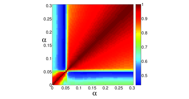
Figure 3: Rank correlation between the two top 300 lists for the dynamic win-lose score with $\beta=1/365$. Pairs of rankings with different values of $\alpha$ are compared.

For the dynamic win-lose scores at $t_{n_{\max}}$, i.e., at the end of the entire period, we calculate $K$ with $k=300$ for different pairs of $\alpha$ and $\beta$ values. The results for $\beta=1/365$ and different values of $\alpha$ are shown in Fig. 3. The top $k$ lists are similar (i.e., $K\geq 0.85$) for any $\alpha$ larger than $\approx 0.06$. This finding is consistent with the fact that the prediction accuracy is high and robust when $\alpha$ falls between $\approx 0.08$ and $\approx 0.2$ (Fig. 2(a)).

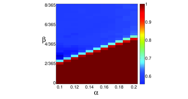
Figure 4: Rank correlation between the two top 300 lists for the dynamic win-lose score with fixed $\alpha$ values. Pairs of ranking, one with $\beta=1/365$ and the other with a general $\beta$ value, are compared.

For fixed values of $\alpha$, the $K$ values between the ranking with $\beta=1/365$ and that with various values of $\beta$ are shown in Fig. 4. $K$ is almost unity at least in the range $0\leq\beta\leq 2/365$. Therefore, removing the assumption of the exponential decay of score in time (i.e., $\beta=0$) little changes the top 300 list. This finding is consistent with the result that the prediction accuracy is almost the same between $\beta=0$ and $\beta=1/365$ if $0.1\leq\alpha\leq 0.2$ (see the previous subsection). Nevertheless, this observation does not imply that we can ignore the temporal aspect of the data. Keeping the order of the games contributes to the performance of prediction, as suggested by the comparison between the prediction results for the dynamic (Fig. 2(a)) and original (Fig. 2(b)) win-lose scores.

Dynamics of scores for individual players

In contrast to the original win-lose score and prestige score, the dynamic win-lose score can track dynamics of the strength of each player. It should be noted that the summation of the scores over the individuals, i.e., $\sum_{i=1}^{N}s_{t_{n}}(i)$, depends on time. In particular, it grows almost exponentially for the parameter values with which the prediction accuracy is high (i.e., $\alpha$ larger than $\approx 0.08$), as shown in Fig. 5. $\sum_{i=1}^{N}s_{t_{n}}(i)$ increases with the number of games, or equivalently, with time because more recent players take more advantage of indirect wins than older players. The increase in $\sum_{i=1}^{N}s_{t_{n}}(i)$ is not owing to the number of players or games observed per year; in fact, the latter numbers do not increase in time [6].

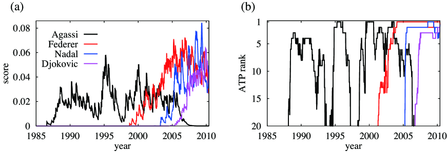
Figure 6: (a) Time courses of normalized win-lose scores for Andre Agassi, Roger Federer, Rafael Nadal, and Novak Djokovic. (b) Time courses of the ATP rankings for the four players.

Therefore, for clarity, we normalize the win-lose score of each player by dividing it by the instantaneous $\sum_{i=1}^{N}s_{t_{n}}(i)$ value. The time courses of the normalized win-lose scores for four renowned players are shown in Fig. 6(a). We set $\alpha=0.13$ and $\beta=1/365$, for which the prediction is approximately the most accurate. The ATP rankings of the four players during the same period are shown in Fig. 6(b) for comparison. The time courses of the dynamic win-lose score and those of the ATP rankings are similar. In particular, the times at which the strength of one player (e.g., Federer) begins to exceed another player (e.g., Agassi) are similar between Figs. 6(a) and 6(b). Figure 6 suggests that the dynamic win-lose score appositely captures rises and falls of these players.

Discussion

We extended the win-lose score for static sports networks [9] to the case of dynamic networks. By assuming that the score decays exponentially in time, we could derive closed online update equations for the win and lose scores. The proposed dynamic win-lose score realizes a higher prediction accuracy than the original win-lose score and the prestige score. It is straightforward to extend the dynamic win-lose score to incorporate factors such as the importance of each tournament or game via modifications of the game matrix $A_{t_{n}}$. We also confirmed the robustness of the ranking against variation in the two parameter values in the model. Finally, the dynamic win-lose score is capable of tracking dynamics of players’ strengths.

It seems that network-based ranking systems are easier to understand and implement, and more scalable than those based on statistical methods. The dynamic win-lose score share these desirable features with static network-based ranking systems.

The applicability of the idea behind the dynamic win-lose score is not limited to the case of the win-lose score. In fact, we implemented a dynamic variant of the prestige score. It even yielded a larger prediction accuracy than the dynamic win-lose score did. This result implies that the idea of network-based dynamic ranking systems may be a powerful approach to assessing strengths of sports players and teams, which fluctuate over time. The dynamic win-lose score is better than our version of the dynamic prestige score in that only the former allows for a set of closed online update equations. Establishing similar update equations for other network-based ranking systems such as the prestige score and the Laplacian centrality (see Introduction) is warranted for future work. Prospective results obtained through this line of researches may be also useful in systematically deriving dynamic centrality measures for temporal networks in general.

Methods

Park & Newman’s win-lose score

The win-lose score by Park and Newman [9] is a network-based static ranking system defined as follows. We assume $N$ players and denote by $A_{ij}$ ($1\leq i,j\leq N$) the number of times that player $j$ wins against player $i$ during the entire period. We let $\alpha$ ($0\leq\alpha<1$) be a constant representing the weight of indirect wins. For example, if player $i$ wins against $j$ and $j$ wins against $k$, $i$ gains score 1 from the direct win against $j$ and score $\alpha$ from the indirect win against $k$. Therefore, the $i$’s win score is equal to $1+\alpha$. If $k$ wins against yet another player $\ell$, the $i$’s win score is altered to $1+\alpha+\alpha^{2}$.

The win scores of the players are given by

$$W= A+\alpha A^{2}+\alpha^{2}A^{3}+\cdots$$

$$= A(I+\alpha A+\alpha^{2}A^{2}+\alpha^{3}A^{3}+\cdots)$$

$$= A(I-\alpha A)^{-1},$$ (11)

$$\bm{w}= W^{\top}\bm{1}=(I-\alpha A^{\top})^{-1}A^{\top}\bm{1},$$ (12)

where $W$ is the $N\times N$ matrix whose $(i,j)$ element represents the score that player $j$ obtains via direct and indirect wins against player $i$, $\bm{w}$ is the $N$ dimensional column vector whose $i$th element represents the win score of player $i$, and $\bm{1}$ is the $N$ dimensional column vector defined by

$$\bm{1}=(1\;1\;\cdots\;1)^{\top}.$$ (13)

We similarly obtain the lose scores of the $N$ players in vector form by replacing $A$ with $A^{\top}$ as follows:

$$\bm{\ell}=(I-\alpha A)^{-1}A\bm{1}.$$ (14)

The total win-lose score is given in vector form by

$$\bm{s}=\bm{w}-\bm{\ell}.$$ (15)

Prestige score

The prestige score of player $i$, denoted by $P_{i}$, is defined by

$$P_{i}=(1-q)\sum_{j=1}^{N}P_{j}\frac{\tilde{w}_{ji}}{s_{j}^{\rm out}}+\frac{q}{N}+\frac{1-q}{N}\sum_{j=1}^{N}P_{j}\delta(s_{j}^{\rm out})\quad(1\leq i\leq N),$$ (16)

where $q$ is a constant, $\tilde{w}_{ji}$ is the number of times player $i$ defeats player $j$ during the entire period (it should be noted that $\tilde{w}_{ji}$ has nothing to do with the win scores denoted by $\bm{w}$ in Eqs. (2) and (12)), $s_{j}^{\rm out}\equiv\sum_{i^{\prime}=1}^{N}\tilde{w}_{ji^{\prime}}$ is equal to the number of losses for player $j$, $\delta(s_{j}^{\rm out})=1$ if $s_{j}^{\rm out}=0$, and $\delta(s_{j}^{\rm out})=0$ if $s_{j}^{\rm out}\geq 1$. The normalization is given by $\sum_{i=1}^{N}P_{i}=1$. We set $q=0.15$, as in [6], and also $q=0.05$ and $q=0.30$.

To define a dynamic variant of the prestige score, we let $\tilde{w}_{ij}$ used in Eq. (16) depend on time. We define $\tilde{w}_{ij}$ at time $t$ by

$$\tilde{w}_{ji}\equiv\sum_{n}A_{t_{n}}(j,i)e^{-\beta(t-t_{n})},$$ (17)

where $A_{t_{n}}(j,i)$ is the $(j,i)$ element of the win-lose matrix $A_{t_{n}}$, and the summation over $n$ is taken over the games that occur before time $t$. Substituting Eq. (17) in Eq. (16) yields the dynamic prestige score $P_{i}$ ($1\leq i\leq N$) at time $t$. We set $\beta=1/365$, which is the same value as that used for the dynamic win-lose score.

Data

We collected the data from the website of ATP [23]. Except when we compared the prediction accuracy for the dynamic win-lose score with that for the ATP rankings, we used single games in ATP World Tour tournaments recorded on this website. The data set contains 137842 singles games from December 1972 to May 2010 and involves 5039 players that participated in at least one game. Because the source of our data set is the same as that of Radicchi’s data set [6] and the period of the data is similar, the number of games contained in our data and that in Radicchi’s are close to each other.

In the comparison between the dynamic win-lose score and the ATP rankings, we used all the types of single games recorded on the website of ATP. They include the games belonging to ATP Challenger Tours and ITF Futures tournaments in addition to ATP World Tour tournament games. We used this data set because it corresponds to the games on which the calculation of the ATP rankings is based. The ATP rankings are not available on a regular basis in early years. Therefore, we used the data from July 23, 1984 to August 15, 2011. The data set contains 330796 games and involves 13077 players that participated in at least one game.

Parameter values for the dynamic win-lose score

A guiding principle for setting the parameter values of a ranking system is to select the values that maximize the performance of prediction [22, 19]. Instead, we set $\alpha$ and $\beta$ as follows.

In the original win-lose score, it is recommended that $\alpha$ is set to the value smaller than and close to the inverse of the largest eigenvalue of $A$ [9]. If $\alpha$ exceeds this upper limit, the original win-lose score diverges. For our data, the upper limit according to this criterion is equal to $1/206.80=0.0048355$. However, the dynamic win-lose score converges irrespective of the values of $\alpha$ and $\beta$ for the following reason. For expository purposes, let us assign different nodes to the same player at different times $t_{n}$ ($1\leq n\leq n_{\max}$). Then, Eq. (1) implies that any link in the network, which represents a game at time $t_{n}$, is directed from the winner at $t_{n}$ to the loser at $t_{n}$ or earlier times. Because there is no time-reversed link (i.e., from $t_{n}$ to $t_{n^{\prime}}$, where $t_{n}<t_{n^{\prime}}$) and any pair of players play at most once at any $t_{n}$, the network is acyclic. The upper limit of $\alpha$ is infinite when the network is acyclic [9]. On the basis of this observation, we examine the behavior of the dynamic win-lose score for various values of $\alpha$.

In the official ATP ranking, the score of a player is calculated from the player’s performance in the last 52 weeks $\approx$ one year [23]. The results of the games in this time window contribute to the current ranking of the player with the same weight if the other conditions are equal. The dynamic win-lose score uses the results of all the games in the past, and the contribution of the game decays exponentially in time. By equating the contribution of a single game in the two ranking systems, we assume $1\times 365=\int_{0}^{\infty}e^{-\beta t}dt$, which leads to $\beta=1/365$. In Results, we also investigated the robustness of the ranking results against variations in the $\alpha$ and $\beta$ values.

Author contributions

N.M. designed the research; S.M. contributed the computational results; S.M. and N.M. discussed the results; N.M. wrote the paper.

Additional information

Competing financial interests: The author declares no competing financial interests.

Figure 5: Dynamics of the summation of the scores (i.e., $\sum_{i=1}^{N}s_{t_{n}}(i)$). The lines correspond to $\alpha=0.15$ (top), 0.13, 0.1, 0.08, 0.05, and $10^{-5}$ (bottom). The results for $\alpha=0$ are not shown because $\sum_{i=1}^{N}s_{t_{n}}(i)$ often takes negative values.

References

- [1] Stefani, R. T. Survey of the major world sports rating systems. J. Appl. Stat. 24, 635–646 (1997).
- [2] Daniels, H. E. Round-robin tournament scores. Biometrika 56, 295–299 (1969).
- [3] Moon, J. W. & Pullman, N. J. On generalized tournament matrices. SIAM Rev. 12, 384–399 (1970).
- [4] Borm, N. E., Brink, R. V. D. & Slikker, M. An iterative procedure for evaluating digraph competitions. Ann. Operat. Res. 109, 61–75 (2002).
- [5] Saavedra, S., Powers, S., McCotter, T., Porter, M. A. & Mucha, P. J. Mutually-antagonistic interactions in baseball networks. Physica A 389, 1131–1141 (2010).
- [6] Radicchi, F. Who is the best player ever? A complex network analysis of the history of professional tennis. PLoS ONE 6, e17249 (2011).
- [7] Callaghan, T., Mucha, P. J. & Porter, M. A. The bowl championship series: a mathematical review. Notices of the Am. Math. Soc. 51, 887–893 (2004).
- [8] Herings, P. J. J., van der Laan, G. & Talman, D. The positional power of nodes in digraphs. Soc. Choice Welfare 24, 439–454 (2005).
- [9] Park, J. & Newman, M. E. J. A network-based ranking system for US college football. J. Stat. Mech. P10014 (2005).
- [10] Holme, P. & Saramäki, J. Temporal networks. Phys. Rep. 519, 97–125 (2012).
- [11] Tang, J., Musolesi, M., Mascolo, C., Latora, V. & Nicosia, V. Analysing information flows and key mediators through temporal centrality metrics. In Proceedings of the 3rd Workshop on Social Network Systems (2010).
- [12] Pan, R. K. & Saramäki, J. Path lengths, correlations, and centrality in temporal networks. Phys. Rev. E 84, 016105 (2011).
- [13] Grindrod, P., Parsons, M. C., Higham, D. J. & Estrada, E. Communicability across evolving networks. Phys. Rev. E 83, 046120 (2011).
- [14] Elo, A. E. The Rating of Chess Players, Past & Present (Arco, New York, 1978).
- [15] Bradley, R. A. Science, statistics, and paired comparisons. Biometrics 32, 213–232 (1976).
- [16] Glickman, M. E. Paired comparison models with time-varying parameters. PhD Dissertation. Department of Statistics, Harvard University, Cambridge (1993).
- [17] Fahrmeir, L. & Tutz, G. Dynamic stochastic models for time-dependent ordered paired comparison systems. J. Amer. Stat. Asso. 89, 1438–1449 (1994).
- [18] Glickman, M. E. Parameter estimation in large dynamic paired comparison experiments. J. R. Stat. Soc. Ser. C 48, 377–394 (1999).
- [19] Knorr-Held, L. Dynamic rating of sports teams. J. R. Stat. Soc. Ser. D 49, 261–276 (2000).
- [20] Coulom, R. Whole-history rating: a Bayesian rating system for players of time-varying strength. LNCS 5131, 113–124 (2008).
- [21] Herbrich, R., Minka, T. & Graepel, T. TrueSkillTM: a Bayesian skill rating system. Advances in Neural Information Processing Systems 19, 569–576 (2007).
- [22] Dixon, M. J. & Coles, S. G. Modelling association football scores and inefficiencies in the football betting market. J. R. Stat. Soc. Ser. C 46, 265–280 (1997).
- [23] http://www.atpworldtour.com (date of access: October 1, 2011).
- [24] Martinich, J. College football rankings: do the computers know best? Interfaces 32, 85–94 (2002).
- [25] Ben-Naim, E., Vazquez, F. & Redner, S. Parity and predictability of competitions. J. Quantitative Analysis in Sports 2 (4), article 1 (2006).
- [26] Lundh, T. Which ball is the roundest? — a suggested tournament stability index. J. Quantitative Analysis in Sports 2 (3), article 1 (2006).
- [27] Park, J. Diagrammatic perturbation methods in networks and sports ranking combinatorics. J. Stat. Mech. P04006 (2010).
- [28] Coleman, B. J. Minimizing game score violations in college football rankings. Interfaces 35, 483–496 (2005).
- [29] Brin, S. & Page, L. Anatomy of a large-scale hypertextual web search engine. Proceedings of the Seventh International World Wide Web Conference 107–117 (1998).
- [30] Kendall, M. G. A new measure of rank correlation. Biometrika 30, 81–93 (1938).
- [31] Fagin, R., Kumar, R. & Sivakumar, D. Comparing top lists. SIAM J. Disc. Math. 17, 134–160 (2003).
- [32] McCown, F. & Nelson, M. L. Agreeing to disagree: search engines and their public interfaces. In Proceedings of the 7th ACM/IEEE-CS Joint Conference on Digital Libraries, 309–318 (2007).
Acknowledgments
We thank Mikio Ogawa for the assistance of data collection, Juyong Park for valuable discussion, Taro Takaguchi for critical reading of the manuscript, and the Association of Tennis Professionals for making the data set used in the present study publicly available. We acknowledge financial supports provided through Grants-in-Aid for Scientific Research (No. 23681033) and Innovative Areas “Systems Molecular Ethology”(No. 20115009)) from MEXT, Japan. This research is also supported by the Aihara Project, the FIRST program from JSPS, initiated by CSTP.