A Numerical Algorithm for Singular Optimal LQ Control Systems

Abstract.

A numerical algorithm to obtain the consistent conditions satisfied by singular arcs for singular linear-quadratic optimal control problems is presented. The algorithm is based on the presymplectic constraint algorithm (PCA) by Gotay-Nester [11, 26] that allows to solve presymplectic hamiltonian systems and that provides a geometrical framework to the Dirac-Bergmann theory of constraints for singular Lagrangian systems [9]. The numerical implementation of the algorithm is based on the singular value decomposition that, on each step allows to construct a semi-explicit system. Several examples and experiments are discussed, among them a family of arbitrary large singular LQ systems with index 3 and a family of examples of arbitrary large index, all of them exhibiting stable behaviour.

1. Introduction

Singular problems in optimal control problems and in the calculus of variations have been widely considered from different perspectives. A singular perturbation approach has been often the preferred approach to singular optimal control theory (see for instance [15, 16, 22] and references therein). More recently Jurdjevic has proposed a different viewpoint by introducing Lie-theoretic methods in the problem [14]. A similar problem in the calculus of variations has had a very different history mainly due to the physical insight derived from its appearance in mechanics and field theory, (see for instance Cariñena [4]). P.A.M. Dirac took a brilliant approach introducing a recursive analysis to extract the integrable or solvable part of the system [9]. Dirac’s approach consists essentially on a recursive consistency scheme where the original system of implicit Euler-lagrange equations obtained from the extremal conditions are restricted to a smaller and smaller subset on state space by imposing the existence of at least one solution to the problem passing through them. Such approach has been adapted to the problem of optimal control by Volkaert [Vo], López and Martínez [19], Guerra [13] and Delgado and Ibort [6] by transforming it into a descriptor system. A geometric version of Dirac’s constraint algorithm was presented by Gotay and Nester [11] for presymplectic systems. This algorithm was extended and generalized later on to more general situations (see for instance [Me05]) arriving to essentially the same geometrical algorithm devised by Rabier and Rehinbold [24] to deal with Differential-Algebraic equations (DAE’s). A variety of ideas and techniques have been developed along the years to analyze DAE’s (see for instance [2], [25] or the recent book [18]) and recently various of these approaches have been applied to singular optimal control problems (see [17], [1] for instance). However the PCA algorithm was proposed for the first time in control theory by [26], and López and Martínez [19], Cortés, de Leon, Martín de Diego and Martínez [5] and it has been discussed by Delgado and Ibort [6, 7, 8] in the specific context of singular control theory. Another form of this algorithm was applied to the LQ singular case by Guerra [13].

In this paper we will concentrate on singular linear-quadratic systems. We will transform such algorithm into a linear algebra problem that can be treated numerically. In [17] the methods developed by Kunkel and Merhmann based on the construction of normal forms were applied to predictor systems and as a particular instance, to singular LQ optimal problems More recently [1] have extended these ideas incorporating to the analysis LQ systems with index 3. Campbell’s differential arrays method can also be applied to singular optimal control problems providing both a description of consistent initial conditions and the differential equation giving the solutions to the problem [2]. A full account of the analysis of linear differential-algebraic equations with variable coefficients is presented that could be applied to general singular LQ systems in [18]. We have chosen however to implement the PCA algorithm to solve singular LQ optimal control systems because, apart that it can lead to computational improvements with respect to the general procedures above, it preserves the structure of the system. The linear DAE’s that are obtained from the analysis of singular LQ systems carry a presymplectic structure (inherited from the canonical symplectic structure on the space of states and coestates). Such structure emerges at the end on the set of consistent states and coestates inducing there a (pre)symplectic structure. The reduced equations are hamiltonian with respect to such structure. The algorithm that will be implemented in the present paper will compute the consistent initial states and the corresponding consistent coestates preserving the structure of the problem even though we will leave the analysis of the reduced hamiltonian equations to a continuation of this work.

The numerical implementation of the algorithm is carefully discussed and a family of examples and experiments are analyzed. We will discuss experiments with large matrices and lower index (2 and 3) and experiments with large index $n-1$, where $n$ is the dimension of the state space exhibiting all of them a remarkable stable behaviour of the algorithm. We must point it out however that in the present state of the analysis of the numerical algorithm it is not possible to prove its backwards stability because it contains repeated products of matrices spoiling such possibility. More refined versions of it will be analyzed elsewhere, with a different handling of rank conditions that will improve its efficiency and that will allow for a rigorous error analysis.

The paper will be organized as follows. First we will set up in Section 2 the basic notions for singular optimal problems and the particular instance of LQ systems that we are going to discuss. Section 3 will be devoted to review the PCA algorithm from the slightly wider perspective of quasilinear implicit differential equations and we will discuss the relation of the recursive index of the algorithm to the standard index. In Section 4 we will describe the linear algebraic algorithm corresponding to this problem and in Section 5 we will describe its numerical stability properties by means of various experiments.

2. Constraint algorithms for singular LQ systems

As it was stated in the introduction we will concentrate on the study of LQ optimal control systems. We will discuss the problem of finding $C^{1}$-piecewise smooth curves $\gamma(t)=(x(t),u(t))$ satisfying the linear control equation:

$$\dot{x}^{i}=A^{i}_{j}\,x^{j}+B^{i}_{a}\,u^{a},$$ (1)

and minimizing the objective functional:

$$S(\gamma)=\int_{t_{0}}^{T}L(x(t),u(t))\,dt,$$ (2)

where the quadratic Lagrangian $L$ has the form:

$$L(x,u)=\frac{1}{2}Q_{ij}\,x^{i}\,x^{j}+N_{ia}\,x^{i}\,u^{a}+\frac{1}{2}R_{ab}\,u^{a}\,u^{b},$$ (3)

subjected to fixed endpoints conditions: $x(t_{0})=x_{0}$, $x(T)=x_{T}$ (however we must point it out that the chosen endpoints conditions are not going to be relevant for the analysis to follow, hence they can be replaced by more general ones without altering the results presented in this paper).

The coordinates $x^{i}$, $i=1,\ldots,n$, describe points $x\in{\hbox{{\hbox{{\black R}}}}}^{n}$ in state space and $u^{a}$, $a=1,\ldots,m$, are control coordinates defined on the linear control space ${\hbox{{\hbox{{\black R}}}}}^{m}$. The matrices $A$, $B$, $Q$, $N$ and $R$ will be considered to be constant for simplicity. Again we must stress that the algorithm that we are going to discuss can be applied without difficulty to the time-dependent situtation, however the numerical implementation becomes much more involved, so we have chosen to discuss it just for time-independent systems in order to gain clarity and a better understanding of the experiments and their stability properties.

It is well known that normal etxtremals to this problem are provided by Pontryagin’s Maximum Principle [23]:

The curve $\gamma(t)=(x(t),\,u(t))$ is a normal extremal trajectory if there exists a lifting $(x(t),p(t))$ of $x(t)$ to the costate space ${\hbox{{\hbox{{\black R}}}}}^{n}\times{\hbox{{\hbox{{\black R}}}}}^{n}$ satisfying Hamilton’s equations:

$$\dot{x}^{i}=\frac{\partial H}{\partial p_{i}},\quad\quad\dot{p}_{i}=-\frac{\partial H}{\partial x^{i}},$$ (4)

where $H$ is Pontryagin’s Hamiltonian function:

$$H(x,p,u)=p_{i}\,(A^{i}_{j}\,x^{j}+B^{i}_{a}\,u^{a})-L(x,u),$$ (5)

and the set of conditions:

$$\phi^{(1)}_{\ \ a}(x,p,u):=\frac{\partial H}{\partial u^{a}}=p_{i}\,B^{i}_{a}-N_{ia}\,x^{i}-R_{ab}\,u^{b}=0.$$ (6)

We will call conditions in Eq. (6) primary constraints. Thus, trajectories solution to the optimal control problem must lie in the linear submanifold:

$$M_{1}=\{(x,p,u)\in M_{0}|~{}\phi^{(1)}_{\ \ a}(x,p,u)=0\},$$ (7)

where $M_{0}=\{\,(x,p,u)\in{\hbox{{\hbox{{\black R}}}}}^{2n+m}\,\}$ denotes the total space of the system.

If $(x(t),p(t),u(t))$ is a solution of the optimal problem, then its derivative must satisfy:

$$\dot{x}^{i} = \frac{\partial H}{\partial p_{i}}(x,p,u)=A^{i}_{j}\,x^{j}+B^{i}_{a}\,u^{a},$$ (8)

$$\dot{p}_{i} = -\frac{\partial H}{\partial x^{i}}(x,p,u)=-p_{j}A^{j}_{i}+Q_{ij}x^{j}+N_{ia}u^{a},$$ (9)

$$\dot{u}^{a} = C^{a}(x,p,u),$$ (10)

together with $\dot{\phi}^{(1)}_{\ \ a}(x,p,u)=0$, this is,

$$\frac{\partial\phi^{(1)}_{\ \ a}}{\partial x^{i}}\frac{\partial H}{\partial p_{i}}-\frac{\partial\phi^{(1)}_{\ \ a}}{\partial p_{i}}\frac{\partial H}{\partial x^{i}}+\frac{\partial\phi^{(1)}_{\ \ a}}{\partial u^{b}}\,C^{b}=0.$$

A simple computation shows us that if the system is regular, that is, if the matrix:

$$R_{ab}=\frac{\partial^{2}H}{\partial u^{a}\partial u^{b}}$$

is invertible in $M_{1}$, then there exists an optimal feedback condition solving Equation (6),

$$u^{b}=(R^{-1})^{ab}\,(p_{i}B^{i}_{\,a}-N_{ia}x^{i}).$$ (11)

Then we obtain for Eq. (10):

$$\dot{u}^{b} = (R^{-1})^{ab}(\dot{p}_{i}B^{i}_{a}-N_{ia}\dot{x}^{i})=$$

$$= (R^{-1})^{ab}\left((-p_{j}A^{j}_{i}+Q_{ij}x^{j}+N_{id}u^{d})B^{i}_{a}-N_{ia}(A^{i}_{j}\,x^{j}+B^{i}_{d}\,u^{d})\right).$$

Notice that in this case $\dot{\phi}^{(1)}_{\ \ a}$ vanishes automatically on $M_{1}$.

However, for singular optimal LQ systems, this is, when $R_{ab}$ is not an invertible matrix, it may occur that at some points $(x_{0},p_{0},u_{0})$ satisfying the primary constraint Eq. (6), that solutions of (4) starting at them will not be contained in $M_{1}$ for $t>0$ for any $u$. Because Eqs. (4)-(6) must be satisfied along optimal paths, we must consider only as initial conditions only those points for which there is at least a solution of (4) contained in $M_{1}$ starting from them. Such subset is defined by the following conditions:

$$\mathrm{There~{}exists~{}}C\mathrm{~{}such~{}that~{}}\phi^{(2)}_{\ \ a}:=\dot{\phi}^{(1)}_{\ \ a}=0,$$ (12)

where the derivative is taken in the direction of Eq. (4) and $\dot{u}=C$. The subset obtained, that we will denote by $M_{2}$, is again a linear submanifold of $M_{1}$ (this is also true in the time-dependent case) and we shall denote the functions defining $M_{2}$ in $M_{1}$ by $\phi^{(2)}_{\ \ a}$. We will call them secondary constraints. Notice that, in the case of more general endpoint conditions, that would involve considering end-time conditions on the coestate variables $p_{i}$, the same condition Eq. (12) would apply by changing now the derivative of $p_{i}$ by the derivative along Eq. (4) obtained by time reversing $t\mapsto-t$.

Clearly the argument goes on and we will obtain in this form a family of linear submanifolds defined recursively as follows:

$$M_{k+1}=\{(x,p,u)\in M_{k}\mid\,\exists\ C~{}{\mbox{such that}}~{}\phi^{(k+1)}_{\ \ \ \ \ a}:=\dot{\phi}^{(k)}_{\ \ a}\,(x,p,u)=0\}.$$ (13)

Eventually the recursion will stop and $M_{r}=M_{r+1}=M_{r+2}=\dots$, for certain finite $r$. We will call the number of steps $r$ of the algorithm before it stabilizes the recursive index of the problem. In this way we obtain an invariant linear submanifold,

$$M_{\infty}=\bigcap_{k\geq 0}\,M_{k},$$ (14)

that will be called the final constraint submanifold of the problem and by construction it consists on the set of consistent initial condition for the DAE Eqs. (4)-(6). The geometrical analysis of this algorithm shows that this number $r$ does not depends on the coordinate system and constitutes a intrinsic property of the system. Notice also that for general singular systems, this index may vary in principle from point to point. However this is not the case for singular linear systems as we will see in next section where we will discuss for completeness the relation between the recursive index $r$ and the index of linear DAEs.

As it was stressed in the introduction, this algorithm constitutes both an adapted version of the reduction algorithm for DAEs [24, 25] and the Presymplectic Constraint Algorithm (PCA). The DAE system above however has an additional structure because it is a presymplectic system. The PCA algorithm not only determines the consistent initial conditions for the corresponding DAE, but in addition it provides the explicit form of the reduced Hamiltonian equations by computing the so called Dirac brackets of the system. Such brackets are obtained directly from the sequence of $k$-ary constraints $\phi^{(k)}_{\ \ a}$. In this sense this algorithm is structured and preserves the main structure of the system along its steps. We will just proceed to the numerical implementation of this algorithm in its present form leaving the construction (and integration) of the reduced dynamical system to subsequent articles.

3. The Kronecker and recursive index for linear DAEs

As it was indicated before we will show for completeness the relation of the recursive index with the strangeness and differential indexes of the general theory of DAE’s. Because of the simplicity of the problem at hand it will suffice to compute the Kroneker index of the matrix pencil defining the system. Thus, we consider an (autonomous) quasilinear differential–algebraic equation (DAE) of the form

$$A(x)\dot{x}=B(x),$$ (15)

$x\in{\hbox{{\hbox{{\black R}}}}}^{n}=M_{0}$, where $A(x),\,B(x)\colon{\hbox{{\hbox{{\black R}}}}}^{n}\to F$ and $F$ is an auxiliary linear space (see [12] and the references therein for a geometrical treatment of DAEs). Because the DAE above has no additional structures the PCA becomes particularly simply and completely equivalent to the differential reduction by Rabier and Reinholt [Ra96]. Even more, it can be written in the extremely simple form that follows. If $A(x)$ is regular, we can solve explicitly $\dot{x}$ and the DAE becomes an ordinary differential equation. If $A(x)$ is not regular for some $x\in M_{0}$ we have to impose the constraints algorithm. We shall define $M_{1}$ as the set of points in $M_{0}$ such that $B(x)\in\hbox{{\rm Im}}\,A(x)$. Hence if $x\in M_{1}$ then $\forall\mu\in\ker\,A(x)^{*}\subset F^{*}$ it must be satisfied $\left<\mu,B(x)\right>=0$, where $A^{*}$ denotes the adjoint application of $A$. In general,

$$M_{k+1}=\{x\in M_{k}|~{}B_{k}(x)\in\hbox{{\rm Im}}\,A_{k}(x)\},$$ (16)

where $B_{k}=\left.B\right|_{M_{k}};$ $A_{k}=\left.A\right|_{M_{k}}.$ We obtain again

$$M_{k+1}=\{x\in M_{k}|~{}\left<\mu,B_{k}(x)\right>=0,~{}\forall\mu\in\ker\,A_{k}(x)^{*}\}.$$ (17)

In the particular case of constant linear systems, Equation (15) becomes

$$A\cdot\dot{x}=B\cdot x,$$ (18)

where $x,~{}\dot{x}\in{\hbox{{\hbox{{\black R}}}}}^{n};~{}A,~{}B\in{\hbox{{\hbox{{\black R}}}}}^{n\times n},$ and the submanifold $M_{1}$ defined by (16) is given by

$$M_{1}=\{x\in{\hbox{{\hbox{{\black R}}}}}^{n}|~{}B\cdot x\in\hbox{{\rm Im}}\,A\},$$

but this is equivalent to say that for all $z$ verifying $z^{T}\cdot A=0$ then $z^{T}\cdot B\cdot x=0$. If $z_{a},~{}a=1,\ldots,m,$ is a basis of $\ker\,(A^{T})$, we can construct the family of primary constraints as

$$\phi^{(1)}_{\ \ a}(x)=z_{a}^{T}\cdot B\cdot x.$$

If we define the matrix $C^{(1)}:=[z_{1}|\cdots|z_{m}]$, then the family of linear constraints $\{\phi^{(1)}_{\ \ a}\}_{a=1}^{m}$ is equivalent to the following matrix equation

$$C^{(1)T}\cdot B\cdot x=0.$$ (19)

Now the condition $x\in M_{1}$ is equivalent to $x\in\ker\,(C^{(1)T}\cdot B)$. Denoting by $A_{k}$ as the restriction of $A$ to $M_{k},$ we obtain that the linear manifold $M_{k+1}$ is defined recursively as the set of points $x\in M_{k}$ such that

$$C^{(k+1)T}\cdot B\cdot x=0,$$ (20)

where the columns of $C^{(k+1)}$ generates the kernel of the matrix $A_{k}$.

Let $A\cdot\dot{x}=B\cdot x$ be a constant implicit differential–algebraic system. We will recall that the system is regular in the Kronecker sense if the matrix pencil $A\lambda-B$, $\lambda\in{\hbox{{\hbox{{\black C}}}}}$, is regular, i.e., if the set of solutions of the characteristic equation $p(\lambda)=\det(A\lambda-B)=0$ is finite.

Moreover if the pencil is regular in the Kronecker sense, then there exists regular matrices $E$, $F$ such that [10]:

$$EAF=\left[\begin{array}[]{c|c}I&0\\ \hline\cr 0&N\end{array}\right];~{}~{}EBF=\left[\begin{array}[]{c|c}W&0\\ \hline\cr 0&I\end{array}\right],$$ (21)

where $N$ is a nilpotent matrix with index $\nu$. In such case we will say that the index of the implicit differential-algebraic system given by Equation (18) is $\nu$ (see [18] for a thourough discussion of the subject). The relation of the recursive index to the index of the DAE is given by the following result:

Theorem 1.

The index $\nu$ of the regular constant implicit differential-algebraic system $A\dot{x}=Bx$ coincides with the number of steps of the recursive constraint algorithm minus one:

$$\mathit{number~{}of~{}steps~{}}=r=\nu+1.$$ (22)

Proof.

If Equation (18) is a regular system in the sense of Kronecker, there exist regular matrices $E$ and $F$ such that the system becomes

$$\dot{y}_{1} = Wy_{1},$$ (23)

$$N\dot{y}_{2} = y_{2},$$ (24)

where $N$ is nilpotent with index $\nu$ (i.e. $N^{\nu}\neq 0,~{}N^{\nu+1}=0$) and $x=Fy$, together with $y=\left[\begin{array}[]{c}y_{1}\\ \hline\cr y_{2}\end{array}\right]$.

Now we only need to consider the nilpotent part of the system above, Equation (24). Applying the recursive constraint algorithm to it, we obtain the primary constraint submanifold $M_{1}$, given by the primary constraints

$$\phi^{(1)}=C^{(1)T}y_{2},$$

where the columns of $C^{(1)}$ generates the kernel of $N$.

Moreover, Equation (24) implies that $y_{2}\in M_{1}$ if and only if exists $z\in M_{0}$ such that $y_{2}=Nz$, i.e., $y_{2}\in\hbox{{\rm Im}}\,N$. If $y_{2}(t)$ is a curve solution of the equation, it will mean that $y_{2}(t)=Nz(t)$, hence $\dot{y}_{2}(t)=N\dot{z}(t)$ and then $\dot{y}_{2}\in\hbox{{\rm Im}}\,N$. So we have that $y_{2}=N\dot{y}_{2}=NN\dot{z}=N^{2}\dot{z}.$ Then $y_{2}\in M_{2}$ if and only if $y_{2}\in\hbox{{\rm Im}}\,N^{2},$ and this will happen if and only if

$$\phi^{(2)}=C^{(2)T}y_{2}=0,$$

where $C^{(2)}$ generates the kernel of $N^{2},$ thus

$$M_{2}=\left\{y_{2}\in M_{1}|~{}C^{(2)T}y_{2}=0\right\},~{}\mathrm{Lin}\{\mathrm{Col}(C^{(2)})\}=\ker N^{2}.$$

If we proceed recursively, we can observe that $y_{2}\in M_{k+1}$ if and only if $y_{k}\in\hbox{{\rm Im}}\,N^{k}$ and this will take place if and only if $\phi^{(k)}=C^{(k)T}y_{2}=0,$ where the columns of $C^{k}$ generates the kernel of the matrix $N^{k}$. As the matrix $N$ is nilpotent with index $\nu$ we have that

$$\ker\,N\subsetneqq\ker\,N^{2}\subsetneqq\ker\,N^{3}\subsetneqq\cdots\subsetneqq\ker\,N^{\nu}\subsetneqq\ker\,N^{\nu+1}={\hbox{{\hbox{{\black R}}}}}^{m}.$$

So, in each step, the matrix $C^{(k)}$ contains the previous one, $C^{(k-1)}$, as a submatrix,

$$C^{(k)}=[C^{(k-1)}|~{}*~{}].$$

Notice that in the $\nu$–th step we obtain that

$$y_{2}\in\hbox{{\rm Im}}\,N^{\nu}\Longrightarrow y_{2}=N^{\nu}z,$$

so, the next step is $y_{2}=N\dot{y}_{2}=NN^{\nu}\dot{z}=0$ and the final constraint submanifold is $M_{\nu+1}=M_{\infty}=\{y_{2}=0\},$ given by the constraints $y_{2}=0.$ ∎

4. A numerical linear algebra algorithm for singular LQ systems

Now we will adapt the general recursive constraint algorithm stated in Section 2 to the particular instance of singular LQ control systems. Notice that the description of the constrainsts algorithm done in Section 2 does not involves the use of the presymplectic structure, thus it is a plain constraints algorithm for a DAE. We will follow this approach here instead of using the full PCA algorithm because here we are just addressing the problem of determining the set of consistent initial conditions for our problem. The idea that we are going to follow to implement the algorithm is to transform at each step the implicit problem we have into a semi-explicit system. Then, we will not only get the set of constraints defining the set of consistent initial condition but we will have at the same time the set of explicit reduced equations of the system. In this form the algorithm will not provide the Hamiltonian structure of the equations though as it was pointed it out before.

We will discuss now the basic idea of the algorithm from the matrix analysis perspective. We will write down all coordinates as column vectors: $(x,p)\in{\hbox{{\hbox{{\black R}}}}}^{n}\times{\hbox{{\hbox{{\black R}}}}}^{n}$ and $u\in{\hbox{{\hbox{{\black R}}}}}^{m}$. The control equation and the lagrangian density have the form already described in Section 2, now written in matrix notation reads as

$$\dot{x} = Ax+Bu,$$ (25)

$$L = \frac{1}{2}x^{T}Qx+x^{T}Nu+\frac{1}{2}u^{T}Ru,$$ (26)

with $A,~{}Q\in{\hbox{{\hbox{{\black R}}}}}^{n\times n}$, $B,~{}N\in{\hbox{{\hbox{{\black R}}}}}^{n\times m}$ and $R\in{\hbox{{\hbox{{\black R}}}}}^{m\times m}$. The Pontryagin’s Hamiltonian becomes:

$$H(x,p,u)=p^{T}Ax+p^{T}Bu-\frac{1}{2}x^{T}Qx-x^{T}Nu-\frac{1}{2}u^{T}Ru.$$ (27)

Using these notations the equations of motion (8)-(10) become:

$$\dot{x} = \frac{\partial H}{\partial p^{T}}=Ax+Bu,$$ (28)

$$\dot{p} = -\frac{\partial H}{\partial x^{T}}=-A^{T}p+Qx+Nu,$$ (29)

$$\dot{u} = C,$$ (30)

and the column primary constraint vector is given by:

$$\phi^{(1)}:=-N^{T}x+B^{T}p-Ru.$$ (31)

We must notice that when applying the recursive constraint algorithm to the problem above, that all the constraints thus obtained will be linear. Then we can writet them at each step $k$ of the algorithm as:

$$\phi^{(k)}(x,p,u):=\sigma^{(k)}x+\beta^{(k)}p+\rho^{(k)}u,$$ (32)

with matrices $\sigma^{(k)},\beta^{(k)}\in{\hbox{{\hbox{{\black R}}}}}^{r_{k}\times n}$, $\rho^{(k)}\in{\hbox{{\hbox{{\black R}}}}}^{r_{k}\times m}$, for some $r_{k}\in{\hbox{{\hbox{{\black N}}}}}$. Notice that:

$$\sigma^{(1)}=-N^{T},\quad\beta^{(1)}=B^{T},\quad\rho^{(1)}=-R.$$

The matrix equations

$$\phi^{(1)}=0;\ldots;\phi^{(k)}=0,$$

define the linear manifolds $M_{k}$ obtained by applying the recursive constraint algorithm. Thus the matrices $\sigma^{(k)}$, $\beta^{(k)}$, $\rho^{(k)}$ completely characterize the constraints $\phi^{(k)}$. We will store these matrices in a block structured matrix $\Phi$ whose $k$–th row, $\Phi(k,:)$, will be given by $\left[\begin{array}[]{c|c|c}\sigma^{(k)}&\beta^{(k)}&\rho^{(k)}\end{array}\right].$

If $R$ is a regular matrix, then there exists an optimal feedback and the control variables are uniquely determined. However, if $R$ is singular we must apply the recursive constraint algorithm. As we have discussed above, the first step of the algorithm amounts to study the stability of the primary constraint $\phi^{(1)}$, i.e., to determine for which points $(x,p,u)$ there exists a vector $C\in{\hbox{{\hbox{{\black R}}}}}^{m}$ satisfying

$$\dot{\phi}^{(1)}=\sigma^{(1)}\dot{x}+\beta^{(1)}\dot{p}+\rho^{(1)}C=0,$$ (33)

with $C=\dot{u}$. Because $\rho^{(1)}$ is singular, the linear system obtained from it

$$\rho^{(1)}C=b(x,p,u),$$

with $b(x,p,u)=-\sigma^{(1)}\dot{x}-\beta^{(1)}\dot{p}$, will not always have solution. However, given the dependence of $(x,p,u)$ on the inhomogeneous part of the linear equation, we can determine for which values of them the system will have solution. For those points $(x,p,u)$ such that a solution exists, i.e., such that there exists $C\in{\hbox{{\hbox{{\black R}}}}}^{m}$ with $\dot{\phi}^{(1)}(x,p,u)=0$, we will obtain a partial optimal feedback. The remaining equations will impose further conditions on the points $(x,p,u)$ where we can expect to find solutions to the original optimal control problem. That part will constitute what we were calling before the secondary constraints of the problem.

We will obtain this separation between the partial optimal feedback and the secondary constraints by using the singular value decomposition (SVD) of $\rho^{(1)}$. There exists two unique orthogonal matrices, $U^{(1)},~{}V^{(1)}$, and real numbers $s_{1}^{(1)}\geq s_{2}^{(1)}\geq\dots\geq s_{r_{1}}^{(1)}>0,$ the singular values of $\rho^{(1)}$, such that:

$$\rho^{(1)}=U^{(1)}\,\Sigma^{(1)}\,V^{(1)\,T}=U^{(1)}\,\left[\begin{array}[]{c c c|c}s_{1}^{(1)}&&&\\ &\ddots&&0\\ &&s_{r_{1}}^{(1)}&\\ \hline\cr&0&&0\end{array}\right]\,V^{(1)\,T}.$$

Redefining the variables $u^{(1)}=V^{(1)\,T}u$, then $\dot{u}^{(1)}=V^{(1)\,T}\dot{u}=V^{(1)\,T}C=C^{(1)},$ and

$$0 = U^{(1)\,T}\,\dot{\phi}^{(1)}=U^{(1)\,T}\left(\sigma^{(1)}\dot{x}+\beta^{(1)}\dot{p}\right)+\Sigma^{(1)}C^{(1)}=$$ (36)

$$= U^{(1)\,T}\left(\sigma^{(1)}\dot{x}+\beta^{(1)}\dot{p}\right)+\left[\begin{array}[]{c|c}\Sigma^{(1)}\,_{r_{1}}&0\\ \hline\cr 0&0\end{array}\right]C^{(1)}=0,$$

where $\Sigma^{(1)}\,_{r_{1}}=\mathrm{diag}(s_{1}^{(1)},\ldots,s_{r_{1}}^{(1)}).$We will split $C^{(1)}$ as $[C_{r_{1}}^{(1)},C_{m-r_{1}}^{(1)}]^{T},$ where $C_{r_{1}}^{(1)}$ are the components $1,\ldots,r_{1},$ of $C^{(1)}$ and $C_{m-r_{1}}^{(1)}$ the $r_{1},\ldots,m,$ ones. We then get a partial feedback for $C_{r_{1}}^{(1)}$ and the new constraint $\phi^{(2)}$:

$$[~{}I_{r_{1}}|~{}~{}~{}~{}0~{}~{}~{}~{}]\,U^{(1)\,T}\left(\sigma^{(1)}\dot{x}+\beta^{(1)}\dot{p}\right)+\Sigma_{r_{1}}^{(1)}C_{r_{1}}^{(1)}=0$$ (37)

and,

$$\phi^{(2)} := [~{}0~{}~{}|~{}I_{m-r_{1}}~{}]\,U^{(1)\,T}\left(\sigma^{(1)}\dot{x}+\beta^{(1)}\dot{p}\right)=$$

$$= [~{}0~{}|~{}I_{m-r_{1}}~{}]\,U^{(1)\,T}\left[(\sigma^{(1)}A+\beta^{(1)}Q)x+(-\beta^{(1)}A^{T})p+(\sigma^{(1)}B+\beta^{(1)}N)u\right]=$$

$$= \sigma^{(2)}x+\beta^{(2)}p+\rho^{(2)}u=0.$$

Iterating the process, given the $k$–th constraint $\phi^{(k)}$ defined in (32), the SVD of the matrix $\rho^{(k)}$ provides orthogonal matrices $U^{(k)}$, $V^{(k)}$, and the new constraint:

$$\phi^{(k+1)}:=\sigma^{(k+1)}x+\beta^{(k+1)}p+\rho^{(k+1)}u,$$

with,

$$\sigma^{(k+1)} = [~{}0~{}|~{}I_{m-r_{k}}~{}]\,U^{(k)\,T}\left(\sigma^{(k)}A+\beta^{(k)}Q\right),$$ (39)

$$\beta^{(k+1)} = [~{}0~{}|~{}I_{m-r_{k}}~{}]\,U^{(k)\,T}\left(-\beta^{(k)}A^{T}\right),$$ (40)

$$\rho^{(k+1)} = [~{}0~{}|~{}I_{m-r_{k}}~{}]\,U^{(k)\,T}\left(\sigma^{(k)}B+\beta^{(k)}N\right).$$ (41)

The recursive relations above can be solved explicitly. First we shall denote as $U^{k}:=[~{}0~{}|~{}I_{m-rk}~{}]\,U^{(k)\,T}$ for each $k$, and then consider the simplified recurrence relations:

$$\widetilde{\sigma}^{(k+1)} = \widetilde{\sigma}^{(k)}A+\widetilde{\beta}^{(k)}Q$$ (42)

$$\widetilde{\beta}^{(k+1)} = -\widetilde{\beta}^{(k)}A^{T}$$ (43)

$$\widetilde{\rho}^{(k+1)} = \widetilde{\sigma}^{(k)}B+\widetilde{\beta}^{(k)}N$$ (44)

Before solving this set of conditions, let us compute the relation of $\widetilde{\sigma}$, $\widetilde{\beta}$ and $\widetilde{\rho}$ with $\sigma$, $\beta$ and $\rho$ respectively. First we will compute such relation for $\beta$. Notice that:

$$\beta^{(1)}=\widetilde{\beta}^{(1)},\quad\beta^{(2)}=U^{1}\left(-\beta^{(1)}A^{T}\right)=U^{1}\widetilde{\beta}^{(2)},$$ (45)

then for $k\geq 2$:

$$\beta^{(k)} = U^{k}\left(-\beta^{(k-1)}A^{T}\right)=$$ (46)

$$= U^{k-1}\cdots U^{2}U^{1}\left(-\widetilde{\beta}^{(k-1)}A^{T}\right)=U^{k-1}\cdots U^{2}U^{1}\widetilde{\beta}^{(k)}.$$

A similar computation shows that:

$$\sigma^{(k+1)}=U^{k}\cdots U^{2}U^{1}\widetilde{\sigma}^{(k+1)},\quad k\geq 1.$$ (47)

Finally, when computing $\rho^{(k+1)}$ we obtain the same result.

$$\rho^{(k+1)}=U^{k}\cdots U^{2}U^{1}\left(\widetilde{\sigma}^{(k)}B+\widetilde{\beta}^{(k)}N\right)=U^{k}\cdots U^{2}U^{1}\widetilde{\rho}^{(k+1)}.$$ (48)

Now expanding Eqs. (42)-(44) we obtain the explicit expression for the matrices $\widetilde{\beta}^{(k)}$:

$$\widetilde{\beta}^{(1)}=B^{T},\quad\widetilde{\beta}^{(k+1)}=(-1)^{k}B^{T}(A^{T})^{k},\quad k\geq 1.$$ (49)

For the matrices $\widetilde{\sigma}^{(k)}$ we get:

$$\widetilde{\sigma}^{(1)}=-N^{T},\quad\widetilde{\sigma}^{(k+1)}=-N^{T}A^{k}+B^{T}\left[\sum_{i=0}^{k-1}(-1)^{i}(A^{T})^{i}QA^{k-1-i}\right],$$ (50)

and, finally for the matrices $\widetilde{\rho}^{(k)}$ we obtain:

$$\widetilde{\rho}^{(1)}~{}~{}~{} = -R,\quad\widetilde{\rho}^{(2)}=-N^{T}B+B^{T}N,$$

$$\widetilde{\rho}^{(k+1)} = -N^{T}A^{k-1}B+(-1)^{k-1}B^{T}(A^{T})^{k-1}N+$$ (51)

$$+B^{T}\left[\sum_{i=0}^{k-2}(-1)^{i}(A^{T})^{i}QA^{k-2-i}\right]B,\quad k\geq 2.$$

We summarize the previous findings in the following theorem:

Theorem 2.

The constraints $\phi^{(k)}=\sigma^{(k)}\,x+\beta^{(k)}\,p+\rho^{(k)}\,u$, of the autonomous LQ singular optimal control problem defined by the matrices $A,~{}P,\in{\hbox{{\hbox{{\black R}}}}}^{n\times n};~{}B,~{}Q,\in{\hbox{{\hbox{{\black R}}}}}^{n\times m};~{}R\in{\hbox{{\hbox{{\black R}}}}}^{m\times m},$

$$\dot{x} = Ax+Bu$$ (52)

$$L = \frac{1}{2}x^{T}Px+x^{T}Qu+\frac{1}{2}u^{T}Ru,$$ (53)

are given by the following formuli:

$$\beta^{(1)} = B^{T},\quad\sigma^{(1)}=-N^{T},\quad\rho^{(1)}=-R,\quad\rho^{(2)}=U^{1}\left(-N^{T}B+B^{T}N\right)$$ (54)

$$\beta^{(k)} = (-1)^{k}U^{k-1}\cdots U^{1}B^{T}(A^{T})^{k-1},\quad k\geq 2,$$ (55)

$$\sigma^{(k)} = U^{k-1}\cdots U^{1}\left(-N^{T}A^{k-1}+B^{T}\left[\sum_{i=0}^{k-2}(-1)^{i}(A^{T})^{i}QA^{k-2-i}\right]\right),k\geq 2,$$ (56)

$$\rho^{(k)} = U^{k-1}\cdots U^{1}\left(-N^{T}A^{k-2}B+(-1)^{k-2}B^{T}(A^{T})^{k-2}N\right.+$$ (58)

$$+\left.B^{T}\left[\sum_{i=0}^{k-3}(-1)^{i}(A^{T})^{i}QA^{k-3-i}\right]B\right),\quad k\geq 3,$$

$$\rho^{(k)} = U^{(k)}\Sigma^{(k)}V^{(k)T},$$ (59)

$$U^{k}~{} = [~{}0~{}|~{}I_{m-r(k)}~{}]\,U^{(k)\,T}.$$ (60)

If we perturb the matrices $A,B,Q,N,R$ into $A+\delta A$, $B+\delta B$, $Q+\delta Q$, $N+\delta N$ and $R+\delta R$ respectively, then the matrices $\beta^{(k)}$, $\sigma^{(k)}$, $\rho^{(k)}$ will be changed into $\beta^{(k)}+\delta\beta^{(k)}$, $\sigma^{(k)}+\delta\sigma^{(k)}$, $\rho^{(k)}+\delta\rho^{(k)}$. Then by using the explicit expressions Eqs. (54)-(60) it is a straigthforward but tedious computation to obtain the following estimates for the conditioning of the numerical problem of computing the matrices $\beta^{(k)}$, $\sigma^{(k)}$, $\rho^{(k)}$ ($k\geq 2$):

$$\frac{||\delta\widetilde{\beta}^{(k)}||}{||\widetilde{\beta}^{(k)}||} \leq (k-1)\kappa_{A}\frac{||\delta A||}{||A||}+\kappa_{B}\frac{||\delta B||}{||B||},$$ (61)

$$\frac{||\delta\widetilde{\sigma}^{(k)}||}{||\widetilde{\sigma}^{(k)}||} \leq \kappa_{A}\frac{||\delta A||}{||A||}+\kappa_{B}\frac{||\delta B||}{||B||}+(k-2)\kappa_{Q}\frac{||\delta Q||}{||Q||}+(k-1)\kappa_{N}\frac{||\delta N||}{||N||},$$ (62)

$$\frac{||\delta\widetilde{\rho}^{(k)}||}{||\widetilde{\rho}^{(k)}||} \leq C\left[(k-1)\kappa_{A}\frac{||\delta A||}{||A||}+\kappa_{B}\frac{||\delta B||}{||B||}+(k-2)\kappa_{Q}\frac{||\delta Q||}{||Q||}+\kappa_{N}\frac{||\delta N||}{||N||}\right]$$ (63)

for some (small) constant $C$. Notice that for $k>1$, the output matrices are not sensitive to variations on the input matrix $R$, which on the other hand is responsible for the launching of the algorithm. Thus after the first step, the singular matrix singular $R$ dissapears from the computations and does not influence anymore the rest of the construction.

However, in spite of the closed expressions obtained above for the constraints of the system, in order to construct the numerical algorithm to compute them, we will not use Eqs. (54)-(60) but rather on we will rely on the recursion Eqs. (39)-(41). The algorithm will halt whenever at the step $k$:

• $\rho^{(k)}$ is regular, then we can obtain an optimal feedback $u=u(x,p)$ and we will substitute it in the equations, or,

• $\phi^{(k)}$ is a linear combination of the previous constraints. In such a case, there will exists a “gauge” freedom, i.e., some of the controls will be not be determined.

Thus, the scheme of the algorithm will be:

Recursive Constraint Algorithm for singular LQ problems  

input $A$, $B$, $Q$, $N$, $R$, $tol$
Build the constraints matrix: $\Phi=[\sigma^{(1)}~{}~{}\beta^{(1)}~{}~{}\rho^{(1)}]$
while	$\hbox{{\rm rank}}(\rho,tol)$ is deficient & $\hbox{{\rm rank}}(\Phi,~{}tol)$ increases
	$(U,\rho,V)=$ SVD($\rho$);  Compute the singular value decomposition of $\rho^{(k)}$
	Compute the iterated matrices $\sigma^{(k+1)},~{}\beta^{(k+1)},~{}\rho^{(k+1)}$
	Build the new constraints matrix: $\Phi=\left[\begin{array}[]{ccc}&\Phi&\\ \sigma^{(k+1)}&\beta^{(k+1)}&\rho^{(k+1)}\end{array}\right]$
	Eliminate the dependent rows of $\Phi$
end while
output $\Phi,$ $k$

 

Note that the rank is computed as a numerical rank with tolerance $tol$.

Pseudocode: “final constraint submanifold”
for linear quadratic optimal control problems  

input $A$, $B$, $Q$, $N$, $R$, $tol$
$\sigma\leftarrow-N^{T};~{}\beta\leftarrow B^{T};~{}\rho\leftarrow-R;$  Initialize the variables $\sigma,~{}\beta,~{}\rho$
$[l,m]\leftarrow$size$(\rho)$;  Initialize the dimension $l\times m$ of $\rho$, $l$=maximum value
$\Phi\leftarrow[\sigma,\beta,\rho];$  Initialize the constraints matrix $\Phi$
$\Phi\leftarrow$ independent rows$(\Phi,~{}tol)$;  Eliminate the dependent rows
$p\leftarrow 0$;  Where $p$ denotes rank($\Phi$), it must be 0 to enter in the boucle
$k\leftarrow 1;$
while rank	($\rho,~{}tol$)$<l~{}\&~{}$rank($\Phi,~{}tol)>$p
	$k\leftarrow k+1;$
	$p\leftarrow$ rank($\Phi$);  Update the rank of $\Phi$
	$r\leftarrow$ rank($\rho,~{}tol$);  Update the rank of $\rho^{(k)}$
	$[l,m]\leftarrow$size($\rho$);  Update the dimensions $l\times m$ of $\rho^{(k)}$
	$[U,\rho,V]\leftarrow$SVD($\rho$);  Singular value decomposition of $\rho^{(k)}$
	$U\leftarrow U^{T}$
	Compute the iterated matrices $\sigma^{(k+1)},~{}\beta^{(k+1)},~{}\rho^{(k+1)}$:
	$\rho\leftarrow~{}U(r+1:l,:)\cdot[\sigma\,B+\beta\,N]$
	$\sigma\leftarrow~{}U(r+1:l,:)\cdot[\sigma\,A+\beta\,Q]$
	$\beta\leftarrow~{}U(r+1:l,:)\cdot[-\beta\,A^{T}]$
	$\Phi\leftarrow\left[\begin{array}[]{c}\Phi\\ \hline\cr\sigma~{}\beta~{}\rho\end{array}\right]$;  Add the new constraints
	$\Phi\leftarrow$ independent rows($\Phi,~{}tol$);  Eliminate the dependent rows
end while
if rank$(\Phi,tol)<=p$
	$k\leftarrow k-1$
end if
output ($\Phi,~{}k$)

 

Pseudocode: “independent rows”
used in the “final constraint submanifold”  

Procedure independent rows($\Phi,~{}tol$)
$[l,c]\leftarrow$ size($\Phi$);  Initialize the dimension $l\times c$ of $\Phi$
if $l\geq$	$~{}1\&~{}\hbox{{\rm rank}}(\Phi,tol)>0$ then
	$F\leftarrow\Phi(1,:)$
	for $i=$	$~{}2:l$
		if rank	$(F,tol)<\hbox{{\rm rank}}\left(\left[\begin{array}[]{c}F\\ \Phi(i,:)\end{array}\right],tol\right)$ then
			$F\leftarrow\left[\begin{array}[]{c}F\\ \Phi(i,:)\end{array}\right]$;  If the row $i$ is linearly independent we will add it
		end if
	end for
else if
	$F\leftarrow[\hskip 5.69054pt]$;   If the matrix has zero rank or it is void, returns the void matrix
end if
$\Phi\leftarrow F$
output $\Phi$

 

5. Examples and numerical experiments

We will discuss here some numerical experiments showing that the numerical algorithm discussed above behave as expected with respect to stability and consistency. The microprocessor used for the numerical computations was Pentium(R), CPU 1.60 GHz, 3.99 MHz, 0.99 GB RAM, and the program used was MATLAB 7.0.0.

We will describe two types of experiments concerning small ($k=3$) and large recursive index respectively. We are constructing a class of problems that is general enough for the purposes of the numerical stability experiments we are going to describe and that we can solve and describe the solution explicitly.

In the small index problem $k=3$, we show that the algorithm is stable with respect to the tolerance used to compute the numerical rank, $tol$, and with respect to perturbations $\delta$ of the data. We will also discuss the dependence with the size, $n$, of the matrices.

For the large index ones, we analyze a problem of index $n-1$, where the algorithm behaves properly with respect to the number of steps, both regarding the tolerance, $tol$, and the perturbation of the data, $\delta$.

Small index problems. Small matrices

Consider the positive semidefinite symmetric $n\times n$ matrix $R$ of rank 1, thus there will exists an orthogonal matrix $U$ such that

$$R=U^{T}R^{\prime}U$$ (64)

such that all elements of $R^{\prime}$ vanish except $R^{\prime}_{11}>0$. State and control spaces are both ${\hbox{{\hbox{{\black R}}}}}^{n}$, and the total space $(x,p,u)$ is ${\hbox{{\hbox{{\black R}}}}}^{3n}$. The matrix $A$ is generic and $B$ is an orthonormal matrix, $B^{T}B=I_{n}$. Finally the objective functional is constructed by using a generic symmetric matrix $Q$, a matrix $N$ of the form $N=BV$ where $V$ is any symmetric matrix and the matrix $R$ described above.

The primary constraints matrix is given by

$$\Phi^{(1)}=\left[\begin{array}[]{c|c|c}-N^{T}&B^{T}&-R\end{array}\right]=\left[\begin{array}[]{c|c|c}-I_{n}&I_{n}&-R\end{array}\right],$$

corresponding to primary constraints

$$\phi^{(1)}=-N^{T}x+B^{T}p-Ru=0,$$

Applying the recursive constraint algorithm we obtain:

$$\dot{\phi}^{(1)}=(-N^{T}A+B^{T}Q)x-B^{T}A^{T}p-(B^{T}N-N^{T}B)u-RC,$$

but the SVD of $R$ is given by Eq. (64), hence the new control coordinate $u^{(1)}$ is given by $u=U^{T}u^{(1)}$ and the matrix $U^{1}$ is just the $(n-1)\times n$ matrix $[0\mid I_{n-1}]U$. Hence multiplying $\dot{\phi}^{(1)}$ on the left by $U^{1}$ and taking into account that $B^{T}N-N^{T}B=0$, we obtain the set of secondary constraints:

$$\phi^{(2)}(x,p,u)=U^{1}(-N^{T}A+B^{T}Q)x-U^{1}B^{T}A^{T}p=0.$$

Now, computing again the derivative of $\phi^{(2)}$ we obtain the equations:

$$\dot{\phi}^{(3)}=U^{1}(-N^{T}A^{2}+B^{T}QA-B^{T}A^{T}Q)x+U^{1}B^{T}(A^{T})^{2}p+U^{1}(B^{T}QB-N^{T}AB-B^{T}A^{T}N)u=0.$$

We observe that the matrix $B^{T}QB-N^{T}AB-B^{T}A^{T}N$ will be invertible for generic $A$, $Q$, $B$ and $V$. For instance if $A=I$, then $\rho^{(3)}$ reduces to:

$$\rho^{(3)}=B^{T}QB-2V.$$

The algorithm will stop here if $\det(B^{T}QB-2V)\neq 0$, this is if $2$ is not an eigenvalue of $V^{1}B^{T}QB$.

The numerical experiment of this problem will consist in applying the algorithm to a collection of matrices built up as a random perturbation of the matrices $A$, $B$, $Q$, $V$ of size $\delta$,

$$\tilde{A}=A+\delta A,\quad\|\delta A\|<\delta,\ldots$$

It is computed for $n=2,\ldots,202$. We analyze the number of steps before the algorithm stabilizes and compute the angle, $\alpha$, between the final constraint submanifold of the perturbed problem and the exact one, this is the error introduced in the problem by the perturbation $\delta A$, etc. Notice that the original matrix $R$ does not affect higher order constraints, hence its numerical influence restricts to launch the algorithm. Perturbations of $R$ will not affect the computation of higher order constraints until it will be of the order of $tol$, then the algorithm will stop at the first iteration because if then the system will be considered to be regular.

Table 1. First experiment (small index, small matrices). $tol=10^{-6}$

n	$\delta$	# exact steps	# steps	codim	$\alpha$/ error
2	1e-016	3	3	4	0.0000000000000014
2	1e-015	3	3	4	0.0000000000000011
2	1e-014	3	3	4	0.0000000000000059
2	1e-013	3	3	4	0.0000000000000857
2	1e-012	3	3	4	0.0000000000010174
2	1e-011	3	3	4	0.0000000000035392
2	1e-010	3	3	4	0.0000000000213074
2	1e-009	3	3	4	0.0000000002366236
2	1e-008	3	3	4	0.0000000095514555
2	1e-007	3	3	4	0.0000000659481913
2	1e-006	3	3	4	0.0000003955805449
– –	– – – – –	– – – – – – – –	– – – –	– – – –	– – – – – – – – – – –
2	1e-005	3	1	2	0.0000048787745951
2	1e-004	3	1	2	0.0000180580284314
2	1e-003	3	1	2	0.0003437294288526
2	1e-002	3	1	2	0.0052691557462037
2	1e-001	3	1	2	0.0558945145125515
n	$\delta$	# exact steps	# steps	codim	$\alpha$/ error
102	1e-016	3	3	304	0.0000000000000071
102	1e-015	3	3	304	0.0000000000000085
102	1e-014	3	3	304	0.0000000000000608
102	1e-013	3	3	304	0.0000000000005422
102	1e-012	3	3	304	0.0000000000060781
102	1e-011	3	3	304	0.0000000000579329
102	1e-010	3	3	304	0.0000000005536516
102	1e-009	3	3	304	0.0000000060825389
102	1e-008	3	3	304	0.0000000579413997
– –	– – – – –	– – – – – – – –	– – – –	– – – –	– – – – – – – – – – –
102	1e-007	3	3	302	0.0000004014308009
102	1e-006	3	3	146	0.0000032681204284
102	1e-005	3	3	108	0.0000322420378538
– –	– – – – –	– – – – – – – –	– – – –	– – – –	– – – – – – – – – – –
102	1e-004	3	1	102	0.0003320360185045
102	1e-003	3	1	102	0.0031921082398989
102	1e-002	3	1	102	0.0340272669549200
102	1e-001	3	1	102	0.1777792824454151
n	$\delta$	# exact steps	# steps	codim	$\alpha$/ error
202	1e-016	3	3	604	0.0000000000000078
202	1e-015	3	3	604	0.0000000000000106
202	1e-014	3	3	604	0.0000000000000809
202	1e-013	3	3	604	0.0000000000007860
202	1e-012	3	3	604	0.0000000000078201
202	1e-011	3	3	604	0.0000000000801147
202	1e-010	3	3	604	0.0000000008647247
202	1e-009	3	3	604	0.0000000081096494
– –	– – – – –	– – – – – – – –	– – – –	– – – –	– – – – – – – – – – –
202	1e-008	3	3	602	0.0000000577669246
202	1e-007	3	3	602	0.0000005902470063
202	1e-006	3	3	262	0.0000048558677195
202	1e-005	3	3	208	0.0000490952628668
– –	– – – – –	– – – – – – – –	– – – –	– – – –	– – – – – – – – – – –
202	1e-004	3	1	202	0.0004788619712676
202	1e-003	3	1	202	0.0046902949060197
202	1e-002	3	1	202	0.0408456670809488
202	1e-001	3	1	202	0.2283913263712342

Table 1. First experiment (small index, small matrices). $tol=10^{-6}$

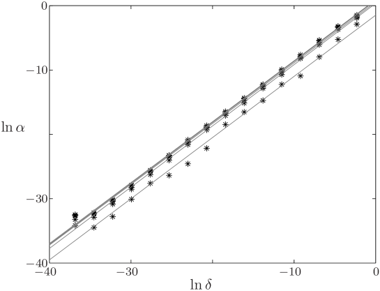
Figure 1. Error for the first experiment (small index, small matrices). $n=2,~{}52,~{}102,~{}152,~{}202.$ Tolerance used for the computations of the numerical rank equal to $10^{-6}$

The results show up that the algorithm works well until perturbations of order of $\delta=10^{-6}$. The least squares approximation of $\ln(\alpha)$ versus $\ln(\delta)$ gives a line of slope $0.95$, which is consistent with $\alpha=O(\delta).$

In Table LABEL:t1 we see that the codimension of the subspace, $codim=3n-1$, that is, the number of rows of the constraints matrix fails at $n=2$ when $\delta$ is of the order of $tol$. However, when $n$ grows $codim$ fails for smaller $\delta$.

Moreover the results show that the algorithm is insensitive to the size of the original matrices. In fact, if we select a fixed value of the perturbation, $\delta=10^{-6}$, and analyze the error for different values of $n$, we obtain Table 2.

Table 2. First experiment (small index, small matrices). $\delta=10^{-9},$ $tol=10^{-6}$

n	$\delta$	# exact steps	# steps	codim	$\alpha/$error
2	1e-009	3	3	4	0.0000000009585285
22	1e-009	3	3	64	0.0000000028931919
42	1e-009	3	3	124	0.0000000034146838
62	1e-009	3	3	184	0.0000000046018755
82	1e-009	3	3	244	0.0000000053815907
102	1e-009	3	3	304	0.0000000055767568
122	1e-009	3	3	364	0.0000000064274692
142	1e-009	3	3	424	0.0000000070707452
162	1e-009	3	3	484	0.0000000072378230
182	1e-009	3	3	544	0.0000000077680372
202	1e-009	3	3	604	0.0000000083969815

Again data obtained indicates heuristically that $\alpha=O(\sqrt{n})$. The least squares approximation of $\ln(\alpha)$ versus $\ln(n)$ gives us an slope of $0.47$.

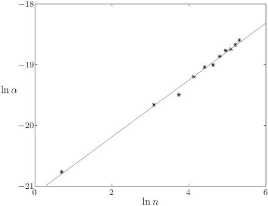
Figure 2. Error for the first experiment (small index, small matrices). $n=2\to~{}202$, $\delta=10^{-6}$, $tol=10^{-6}$

Small index problems. Large matrices

Let us consider the linear–quadratic problem where $A$ is proportional to the identity matrix, $A=\alpha I$, where $\alpha\in{\hbox{{\hbox{{\black R}}}}}$.

The primary constraint will be

$$\phi^{(1)}=\sigma^{(1)}x+\beta^{(1)}p+\rho^{(1)}u=-N^{T}x+B^{T}p-Ru,$$ (65)

the general form of the $(k+1)-th$ constraint will be

$$\phi^{(k+1)} = \sigma^{(k+1)}x+\beta^{(k+1)}p+\rho^{(k+1)}u=[~{}0~{}~{}|~{}I_{m-r_{k}}~{}]\,U^{(k)\,T}\left(\sigma^{(k)}\dot{x}+\beta^{(k)}\dot{p}\right)=$$

$$= [~{}0~{}|~{}I_{m-r_{k}}~{}]\,U^{(k)\,T}\left[(\alpha\sigma^{(k)}+\beta^{(k)}Q)x+(-\alpha\beta^{(k)})p+(\sigma^{(k)}B+\beta^{(k)}N)u\right].$$

Here we use the same notation as in Section 4, that is, after applying the SVD to the matrix $\sigma^{(k)}$, we obtain $\rho^{(k)}=U^{(k)}\,\Sigma^{(k)}\,V^{(k)\,T}$, and $U_{k}:=[~{}0~{}~{}|~{}I_{m-r_{k}}~{}]\,U^{(k)\,T}$. Computing the constraints, we obtain

$$\phi^{(2)} = \sigma^{(2)}x+\beta^{(2)}p+\rho^{(2)}u=U_{1}\left[(\alpha\sigma^{(1)}+\beta^{(1)}Q)x+(-\alpha\beta^{(1)})p+(\sigma^{(1)}B+\beta^{(1)}N)u\right]=$$

$$= U_{1}\left[(-\alpha N^{T}+B^{T}Q)x+(-\alpha B^{T})p+(-N^{T}B+B^{T}N)u\right],$$

$$\phi^{(3)} = \sigma^{(3)}x+\beta^{(3)}p+\rho^{(3)}u=U_{2}\left[(\alpha\sigma^{(2)}+\beta^{(2)}Q)x+(-\alpha\beta^{(2)})p+(\sigma^{(2)}B+\beta^{(2)}N)u\right]=$$

$$= U_{2}U_{1}\left[(-\alpha^{2}N^{T}+\alpha B^{T}Q-\alpha B^{T}Q)x+(\alpha^{2}B^{T})p+(-\alpha N^{T}B+B^{T}QB-\alpha B^{T}N)u\right]=$$

$$= U_{2}U_{1}\left[(-\alpha^{2}N^{T})x+(\alpha^{2}B^{T})p+(-\alpha(N^{T}B+B^{T}N)+B^{T}QB)u\right],$$

$$\phi^{(4)} = \sigma^{(4)}x+\beta^{(4)}p+\rho^{(4)}u=U_{3}\left[(\alpha\sigma^{(3)}+\beta^{(3)}Q)x+(-\alpha\beta^{(3)})p+(\sigma^{(3)}B+\beta^{(3)}N)u\right]=$$

$$= U_{3}U_{2}U_{1}\left[(-\alpha^{3}N^{T}+\alpha^{2}B^{T}Q)x+(-\alpha^{3}B^{T})p+(-\alpha^{2}N^{T}B+\alpha^{2}B^{T}N)u\right].$$

So the constraints matrix will look as

$$\footnotesize\Phi=\left[\begin{array}[]{c|c|c}-N^{T}&B^{T}&-R\\ &&\\ U_{1}\left[-\alpha N^{T}+B^{T}Q\right]&-U_{1}\left[\alpha B^{T}\right]&U_{1}\left[-N^{T}B+B^{T}N\right]\\ &&\\ -U_{2}U_{1}\left[\alpha^{2}N^{T}\right]&U_{2}U_{1}\left[\alpha^{2}B^{T}\right]&U_{2}U_{1}\left[\alpha(-N^{T}B-B^{T}N)+B^{T}QB\right]\\ &&\\ U_{3}U_{2}U_{1}\alpha^{2}\left[-\alpha N^{T}+B^{T}Q\right]&-U_{3}U_{2}U_{1}\alpha^{2}\left[\alpha B^{T}\right]&U_{3}U_{2}U_{1}\alpha^{2}\left[-N^{T}B+B^{T}N\right]\end{array}\right].$$

We can see that the fourth row is related with the second one by $\mathrm{row}_{4}=U_{3}U_{2}\alpha^{2}\mathrm{row}_{2}$, so the algorithm will stop here if it did not do it before.

For the numerical implementation we choose the following matrices: $Q=A=I_{n}\in{\hbox{{\hbox{{\black R}}}}}^{n\times n},$ $B^{T}=(1,\ldots,1)\in{\hbox{{\hbox{{\black R}}}}}^{n\times 1},~{}N^{T}=(0,\ldots,0)\in{\hbox{{\hbox{{\black R}}}}}^{n\times 1},~{}R=0;$ so the constraints matrix will have only three rows

$$\Phi=\left[\begin{array}[]{c|r|c}0,\ldots,0&1,\ldots,\hskip 7.39772pt1&0\\ 1,\ldots,1&-1,\ldots,-1&0\\ 0,\ldots,0&1,\ldots,\hskip 7.39772pt1&n\end{array}\right],$$

where $n$ is the dimension of the matrices $A$ and $Q$. Thus in the third row we obtain optimal feedback and the final constraint submanifold is given by the following equations: $x_{1}+\cdots+x_{n}=p_{1}+\cdots+p_{n}=u=0$.

We apply the numerical algorithm for the previows matrices for $n=1000$, tolerance equal to $10^{-16}$ and we compare the solution obtained with the perturbed matrices: $\tilde{A}=A+\delta A,$ $\|\delta A\|<\delta,$ $\tilde{N}=N+\delta N,$ $\|\delta N\|<\delta$ and $\tilde{B}=B+\delta B,$ $\|\delta B\|<\delta$, where $\delta=10^{-16}\to 10^{-1}$. Again, as the final constraint submanifold of the original problem and the perturbed one must be the same, we measure the angle between them, this is going to be the error, and we show it in Table 3.

Table 3. Second experiment (small index, large matrices). $tol=10^{-16}$

n	$\delta$	# exact steps	# steps	codim	$\alpha$/ error
1000	1e-016	3	3	3	0.00000000000002
1000	1e-015	3	3	3	0.00000000000005
1000	1e-014	3	3	3	0.00000000000010
1000	1e-013	3	3	3	0.00000000000088
1000	1e-012	3	3	3	0.00000000000921
1000	1e-011	3	3	3	0.00000000008945
1000	1e-010	3	3	3	0.00000000094362
1000	1e-009	3	3	3	0.00000000895734
1000	1e-008	3	3	3	0.00000009224712
1000	1e-007	3	3	3	0.00000089770415
1000	1e-006	3	3	3	0.00000934812796
1000	1e-005	3	3	3	0.00008953156206
1000	1e-004	3	3	3	0.00088056539460
1000	1e-003	3	3	3	0.00953194630784
1000	1e-002	3	3	3	0.10128762315235
1000	1e-001	3	3	3	0.80931668976548

Again the data shows that $\alpha=O(\delta)$ and, consistently with the previous results, the slope of the least squares approximation of $\ln(\alpha)$ versus $\ln(\delta)$ is $0.96$.

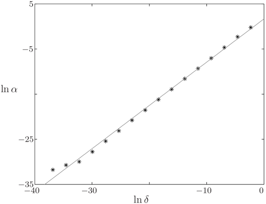
Figure 3. Error for the second experiment (small index, large matrices). $n=1000$. $tol=10^{-16}$

Large index problems

Consider the following problem:

$$A\in{\hbox{{\hbox{{\black R}}}}}^{n\times n},~{}Q=A+A^{T},~{}B\in{\hbox{{\hbox{{\black R}}}}}^{n\times 1},~{}N=B,R=0.$$ (68)

Computing the matrices $\rho^{(1)},~{}\rho^{(2)},\ldots,~{}\rho^{(k)}$, we get

$$\rho^{(1)} = R=0,$$

$$\rho^{(2)} = B^{T}N-N^{T}B=B^{T}B-B^{T}B=0,$$

$$\rho^{(3)} = -N^{T}AB-B^{T}A^{T}N+B^{T}QB=B^{T}[-A-A^{T}+A+A^{T}]B=0,$$

$$\rho^{(4)} = B^{T}[-A^{T}+(-A^{T})^{2}+(A+A^{T})A-A^{T}(A+A^{T})]B=0,$$

$$\vdots$$

$$\rho^{(k+1)} = B^{T}[-A^{k-1}+(-1)^{k-1}(A^{T})^{k-1}+\sum_{i=0}^{k-2}(-1)^{i}(A^{T})^{i}(A+A^{T})A^{k-2-i}]B=$$

$$= B^{T}[-A^{k-1}+(-1)^{k-1}(A^{T})^{k-1}$$

$$+ \sum_{j=1}^{k-1}-(-1)^{j}(A^{T})^{j}A^{k-1-j}+\sum_{j=0}^{k-2}(-1)^{j}(A^{T})^{j}A^{k-1-j}]B=$$

$$= B^{T}[-A^{k-1}+(-1)^{k-1}(A^{T})^{k-1}-(-1)^{k-1}(A^{T})^{k-1}+A^{k-1}]B=0.$$

We obtain that these matrices are always zero and there will not exist optimal feedback. Let us consider now the remaining matrices

$$\sigma^{(1)} = -B^{T},$$

$$\sigma^{(2)} = -B^{T}A+B^{T}(A+A^{T})=B^{T}A^{T},$$

$$\sigma^{(3)} = B^{T}[-A^{2}+(A+A^{T})A-A^{T}(A+A^{T})]=-B^{T}(A^{T})^{2},$$

$$\vdots$$

$$\sigma^{(k+1)} = B^{T}[-A^{k}+\sum_{i=0}^{k-1}(-1)^{i}(A^{T})^{i}(A+A^{T})A^{k-1-i}]=$$

$$= B^{T}[-A^{k}+\sum_{i=0}^{k-1}(-1)^{i}(A^{T})^{i+1}A^{k-1-i}+\sum_{i=0}^{k-1}(-1)^{i}(A^{T})^{i}A^{k-i}]=$$

$$= B^{T}[-A^{k}+\sum_{j=1}^{k}-(-1)^{j}(A^{T})^{j}A^{k-j}+\sum_{j=0}^{k-1}(-1)^{j}(A^{T})^{j}A^{k-j}]=$$

$$= B^{T}[-A^{k}-(-1)^{k}(A^{T})^{k}+A^{k}=(-1)^{k-1}B^{T}(A^{T})^{k}.$$

$$\beta^{(1)} = B^{T},$$

$$\beta^{(2)} = -B^{T}A^{T},$$

$$\vdots$$

$$\beta^{(k+1)} = (-1)^{k}B^{T}(A^{T})^{k}.$$

Hence, we will obtain

$$\beta^{k+1}=-\sigma^{k+1}=(-1)^{k}B^{T}(A^{T})^{k},~{}~{}~{}\rho^{k+1}=0.$$ (69)

and the constraints matrix will look as follows

$$\Phi = \left[\begin{array}[]{cccc}-B^{T}&B^{T}&&0\\ B^{T}A^{T}&-B^{T}A^{T}&&0\\ -B^{T}(A^{T})^{2}&B^{T}(A^{T})^{2}&&0\\ \vdots&\vdots&&\vdots\\ -(-1)^{k}B^{T}(A^{T})^{k}&(-1)^{k}B^{T}(A^{T})^{k}&&0\end{array}\right].$$

Moreover, it is clear from the previous considerations that the algorithm will stop only when at a given step we will obtain a linear combination of the previous rows. Suppose that the minimum polynomial of the matrix $A$ is of degree $q$, then there are two possibilities for the algorithm to stop:

• $B\notin~{}\ker(A^{l}),~{}~{}l=1,\ldots,q$, then the row $q+1$ is a linear combination of the previous ones.

• $B\in~{}\ker(A^{p}),~{}~{}0<p\leq q$, then the row $p+1$ vanish.

We apply the algorithm to a problem where the pair $(A,B)$ is such that $A\in{\hbox{{\hbox{{\black R}}}}}^{n\times n}$ is a nilpotent matrix of index $n$, i.e., $A^{n-1}\neq 0$, $A^{n}=0$, and $B\notin~{}\ker(A^{l})$, $l=1,\ldots,n-1$, i.e., $B^{T}=(1,\ldots,1)\in{\hbox{{\hbox{{\black R}}}}}^{1\times n}$. The index of the algorithm is $k=n$. Perturbing the matrices as: $\tilde{A}=A+\delta A,$ $\|\delta A\|<\delta,$ $\tilde{Q}=\tilde{A}+\tilde{A}^{T},$ $\tilde{B}=B+\delta B,$ $\|\delta B\|<\delta$ , $\tilde{N}=\tilde{B}$ and $\tilde{R}=\delta R,$ $\|\delta R\|<\delta;$ with $\delta=10^{-16}\to 10^{-5}$, we get for $n=20$ with tolerance equal to $10^{-6}$ Table 4.

Table 4. Third experiment (large index). $tol=10^{-6}$

n	$\delta$	# exact steps	# steps	codim	$\alpha$/ error
20	1e-016	20	20	20	0.00000000000001
20	1e-015	20	20	20	0.00000000000002
20	1e-014	20	20	20	0.00000000000001
20	1e-013	20	20	20	0.00000000000004
20	1e-012	20	20	20	0.00000000000021
20	1e-011	20	20	20	0.00000000000652
20	1e-010	20	20	20	0.00000000001940
20	1e-009	20	20	20	0.00000000034574
20	1e-008	20	20	20	0.00000000647005
20	1e-007	20	20	20	0.00000006884601
20	1e-006	20	20	20	0.00000047329442
20	1e-005	20	1	1	0.00000157131430

In this experiment, the value of the slope of the least squares approximation of the data is $0.84$.

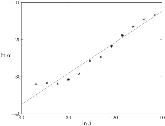
Figure 4. Error for the third experiment (large index). $n=20$, $tol=10^{-6}$

References

• [1] Balla, K., Kurina, G.A., März, R.: Index criteria for differential algebraic equations arising from linear-quadratic optimal control problems. J. Dynamical Control Systems, 12, 289-311 (2006)
• [2] Brenan, K.E., Campbell, S.L., Petzold, L.R.: Numerical Solutions of Initital-Value Problems in Differential-Algebraic Equations. North-Holland (1989)
• [3] Campbell, S. L.: Singular systems of differential equations II. Pitman, London (1982)
• [4] Cariñena, J. F.: Theory of singular lagrangians. Fortschr. Phys. 38, 641–679 (1990)
• [5] Cortés, J., de León, M., Martín de Diego, D., Martínez, S.: Geometric description of vakonomic and nonholonomic dynamics. Comparison of solutions. SIAM J. Control Optim. 45 (5), 1389–1412 (2003)
• [6] Delgado–Téllez, M., Ibort, A.: On the geometry and topology of singular optimal control problems and their solutions. Discrete and Continuous Dynamical Systems, a suplement volume, 223–333 (2003)
• [7] Delgado–Téllez, M., Ibort, A.: A panorama of geometrical optimal control theory. Extracta Mathematicae 18 (2), 129–151 (2003)
• [8] Delgado–Téllez, M.: Métodos geométricos en problemas de control óptimos singulares: fundamentos y aplicaciones. Ph. D. dissertation, Univ. Carlos III de Madrid (2004)
• [9] Dirac, P. A. M.: Generalized hamiltonian dynamics. Canad. J. Math. 2, 129–148 (1950)
• [10] Gantmacher, F. R.: The theory of matrices. Vol. II. Chelsea, New York (1959)
• [11] Gotay, M. J., Nester, J. M., Hinds, G.: Presymplectic manifolds and the Dirac–Bergmann theory of constraints. J. Math. Phys. 19, 2388–2399 (1978)
• [12] Gràcia, X., Muñoz–Lecanda, M. C., Román–Roy, N.: On some aspects of the geometry of differential equations in physics. Int. J. Geometric Methods in Mod. Phys. 1, 265–284 (2004)
• [13] Guerra, M.: Solu ões generalizadas para problemas L-Q singulares. Ph. D. dissertation, Univ. de Aveiro (2001)
• [14] Jurdjevic, V.: Geometric control theory. Cambridge Univ. Press (1997)
• [15] Kokotovic, P. V.: Applications of singular perturbation techniques to control problems. SIAM Review 26, 501–550 (1984)
• [16] Kokotovic, P. V., Khalil, H. K., O’Reilly, J.: Singular perturbation methods in control. Academic Press, London (1986)
• [17] Kunkel, P., Mehrmann, V.: The linear quadratic optimal control problem in linear descriptor systems with variable coefficients. Math. Control Signals Systems, 10, 247-264 (1997).
• [18] Kunkel, P., Mehrmann, V.: Differential-Algebraic Equations. EMS Textbooks in Mathematics, EMS Publ. House (2006)
• [19] López, C., Martínez, E.: Subfinslerian metrics associated to an optimal control problem. SIAM J. Control Opt. 39 (3), 798–811 (2000)
• [20] Mendella, Marmo, Tulczjew (2004)
• [21] Muñoz–Lecanda, M. C., Román–Roy, N.: Lagrangian theory for presymplectic systems. Ann. Inst. Henri Poincaré 57 (1), 27–45 (1992)
• [22] O’Malley Jr, R. E.: Singular perturbations and optimal control. Lect. Notes in Maths. Springer-Verlag, Berlin 680, 170–218 (1978)
• [23] Pontryagin, L. S.,Boltyanskii, V. G., Gamkrelidze, R. V., Mishchenko, E. F.: The mathematical theory of optimal processes. Interscience, N.Y. (1962)
• [24] Rabier, P. J., Rheinboldt, W. C.: A geometric treatment of implicit differential–algebraic equations. J. Diff. Equations. 109, 110–146 (1994)
• [25] Rabier, P. J., Rheinboldt, W. C.: Theoretical and numerical analysis of differential-algebraic equations. Handbook of Numerical Analysis, North Holland/Elsevier VIII, 183–540 (2002)
• [26] Volckaert, K., Aeyels, D.: The Gotay-Nester algorithm in singular optimal control. Proc. 38th Conf. Decision & Control, Phoenix AZ, USA 873-4 (1999)