Color path integral Monte Carlo simulations
of quark-gluon plasma

Abstract

Thermodynamic properties of a strongly coupled quark-gluon plasma (QGP) of constituent quasiparticles is studied by a color path-integral Monte-Carlo simulations (CPIMC). For our simulations we have presented QGP partition function in the form of color path integral with new relativistic measure instead of Gaussian one used in Feynman and Wiener path integrals. For integration over color variable we have also developed procedure of sampling color variables according to the group SU(3) Haar measure. It is shown that this method is able to reproduce the available quantum lattice chromodynamics (QCD) data.

I Introduction

Investigation of properties of the QGP is one of the main challenges of strong-interaction physics, both theoretically and experimentally. Many features of this matter were experimentally discovered at the Relativistic Heavy Ion Collider (RHIC) at Brookhaven. The most striking result, obtained from analysis of these experimental data shuryak08 , is that the deconfined quark-gluon matter behaves as an almost perfect fluid rather than a perfect gas, as it could be expected from the asymptotic freedom. There are various theretical approaches to studying QGP. Each approach has its advantages and disadvantages. The most fundamental way to compute properties of the strongly interacting matter is provided by the lattice QCD Fodor09 ; Csikor:2004ik . Interpretation of these very complicated Monte Carlo computations requires application of various QCD motivated, albeit schematic, models simulating various aspects of the full theory. Moreover, such models are needed in cases when the lattice QCD fails, e.g. at large baryon chemical potentials and out of equilibrium. While some progress has been achieved in the recent years, we are still far away from having a satisfactory understanding of the QGP dynamics.

A semi-classical approximation, based on a point like quasiparticle picture, has been introduced in Levai ; LM105 ; LM109 ; LM110 ; LM111 . It is expected that the main features of non-Abelian plasmas can be understood in simple semi-classical terms without the difficulties inherent to a full quantum field theoretical analysis. Independently the same ideas were implemented in terms of molecular dynamics (MD) Bleicher99 . Recently this MD approach was further developed in a series of works shuryak1 ; Zahed . The MD allowed one to treat soft processes in the QGP which are not accessible by perturbative means.

A strongly correlated behavior of the QGP is expected to show up in long-ranged spatial correlations of quarks and gluons which, in fact, may give rise to liquid-like and, possibly, solid-like structures. This expectation is based on a very similar behavior observed in electrodynamic plasmas thoma04 ; afilinov_jpa03 . This similarity was exploited to formulate a classical nonrelativistic model of a color Coulomb interacting QGP shuryak1 which was numerically analyzed by classical MD simulations. Quantum effects were either neglected or included phenomenologically via a short-range repulsive correction to the pair potential. Such a rough model may become a critical issue at high densities, where quantum effects strongly affects properties of the QGP. To account for the quantum effects we follow an idea of Kelbg kelbg rigorously allowing for quantum corrections to the pair potential . To extend the method of quantum effective potentials to a stronger coupling, we use the original Kelbg potential in the path integral approach, which effectively map the problem onto a high-temperature weakly coupled and weakly degenerate one. This allows one to extend the analysis to strong couplings and is, therefore, a relevant choice for the present purpose.

In this paper we extend previous classical nonrelativistic simulations shuryak1 based on a color Coulomb interaction to the quantum regime. For quantum Monte Carlo simulations of the thermodynamic properties of QGP we have to rewrite the partition function of this system in the form of color path integrals with a new relativistic measure instead of Gaussian one used in Feynman and Wiener path integrals. For integration partition function over color variables we have developed procedure of sampling color quasiparticle variables according to the group SU(3) Haar measure with the quadratic and cubic Casimir conditions. The developed approach self-consistently takes into account the Fermi (Bose) statistics of quarks (gluons). The main goal of this article is to test the developed approach for ability to reproduce known lattice data Fodor09 and to predict other properties of the QGP, which are still unavailable for the lattice calculations. First results of applications of the path integral approach to study of thermodynamic properties of the nonideal QGP have already been briefly reported in Filinov:2009pimc ; Filinov:2010pimc . In this paper we have shown that CPIMC is able to reproduce the QCD lattice equation of state and related thermodynamic functions and also yields valuable insight into the internal structure of the QGP.

Theoretical treatment and hydrodynamic simulations of the experimentally observed expansion of the fireball consisting of quarks and gluons at relativistic heavy-ion collisions suggests knowledge not only thermodynamic but also transport properties of the QGP. Unfortunately the CPIMC method itself is not able to yield transport properties. To simulate quantum QGP transport and thermodynamic properties within unified approach we are going to combine path integral and Wigner (in phase space) formulations of quantum mechanics. The canonically averaged quantum operator time correlation functions and related kinetic coefficients will be calculated according to the Kubo formulas. In this approach CPIMC is used not only for calculation thermodynamic functions but also to generate initial conditions (equilibrium spatial, momentum, spin, flavor and color quasiparticle configurations) for generation of the color trajectories being the solutions of related differential dynamic equations. Correlation functions and kinetic coefficients are calculated as averages of Weyl’s symbols of dynamic operators along these trajectories. The basic ideas of this approach have been published in ColWig11 . Using this approach we are going to calculate diffusion coefficient and viscosity of the strongly coupled QGP. Work on these problems is in progress. In this dynamic approach energy of the quasiparticle system is conserved. In contrast known attempts to use quantum discreet color variable in classical simulations combining dynamic differential equations for quasiparticle coordinates and momenta and discrete color variables results in violation of energy conservation low due to unphysical increase of kinetic energy Levai .

II Thermodynamics of QGP

II.1 Basics of the model

Our model is based on a resummation technique and lattice simulations for dressed quarks, antiquarks and gluons interacting via the color Coulomb potential. The assumptions of the model are similar to those of shuryak1 :

I.

Quasiparticles masses ($m$) are of order or higher than the mean kinetic energy per particle. This assumption is based on the analysis of lattice data Lattice02 ; LiaoShuryak . For instance, at zero net-baryon density it amounts to $m\geq T$, where $T$ is a temperature.

II.

In view of the first assumption, interparticle interaction is dominated by a color-electric Coulomb potential, see Eq. (1). Magnetic effects are neglected as subleading ones.

III.

Relying on the fact that the color representations are large, the color operators are substituted by their average values, i.e. by Wong’s classical color vectors (8D in SU(3)) with the quadratic and cubic Casimir conditions Wong .

IV.

We consider the 3-flavor quark model. Since the masses of the ’up’, ’down’ and ’strange’ quarks extracted from lattice data are still indistinguishable, we assume these masses to be equal. As for the gluon quasiparticles, we allow their mass to be different (heavier) from that of quarks.

The quality of these approximations and their limitations were discussed in shuryak1 . Thus, this model requires the following quantities as a function of temperature and chemical potential as an input:

1.

the quasiparticle masses, $m$, and

2.

the coupling constant $g^{2}$.

All the input quantities should be deduced from the lattice data or from an appropriate model simulating these data.

II.2 Color Path Integrals

Thus, we consider a multi-component QGP consisting of $N$ color quasiparticles representing $N_{g}$ dressed gluon and of various flavors $N_{q}$ dressed quarks and $\bar{N}_{q}$ antiquarks. The Hamiltonian of this system is $\hat{H}=\hat{K}+\hat{U}^{C}$ with the kinetic and color Coulomb interaction parts

$${\hat{K}}=\sum_{i}\sqrt{p^{2}_{i}+m^{2}_{i}(T,\mu_{q})}\qquad{\hat{U}^{C}}=\frac{1}{2}\sum_{i\neq j}\frac{g^{2}(T,\mu_{q})\langle Q_{i}|Q_{j}\rangle}{4\pi|r_{i}-r_{j}|},$$ (1)

Here $i=1,\ldots,N$ is the quasiparticle index, $N=N_{q}+\bar{N}_{q}+N_{g}$, $i$ and $j$ summations run over quark and gluon quasiparticles, 3D vectors $r_{i}$ are quasiparticle spatial coordinates, the $Q_{i}$ denote the Wong’s color variable (8D-vector in the $SU(3)$ group), $T$ is the temperature, and $\mu_{q}$ is the quark chemical potential, $\langle Q_{i}|Q_{j}\rangle$ denote scalar product of color vectors. We use relativistic kinematics, as seen from Eq. (1). Nonrelativistic approximation for potential energy is used to disregard magnetic interaction and retardation in the Coulomb interaction. In fact, the quasiparticle mass and the coupling constant, as deduced from the lattice data, are functions of $T$ and, in general, $\mu_{q}$.

The thermodynamic properties in the grand canonical ensemble with given temperature $T$, baryon ($\mu_{q}$) and strange ($\mu_{s}$) chemical potentials, and fixed volume $V$ are fully described by the grand partition function

$$Z\left(\mu_{q},\mu_{s},\beta,V\right) = \sum_{N_{u},N_{d},N_{s},\bar{N}_{u},\bar{N}_{d},\bar{N}_{s},N_{g}}\frac{\exp\{\mu_{q}(N_{q}-\bar{N}_{q})/T\}\;\exp\{\mu_{s}(N_{s}-\bar{N}_{s})/T\}}{N_{u}!\;N_{d}!\;N_{s}!\;\bar{N}_{u}!\;\bar{N}_{d}!\;\bar{N}_{s}!\;N_{g}!}Z\left(N,V,\beta\right)\text{,}$$ (3)

$$Z\left(N,V,\beta\right)=\sum_{\sigma}\int\limits_{V}dr\;d\mu Q\;\rho(r,Q,\sigma;N_{u},N_{d},N_{s},\bar{N}_{u},\bar{N}_{d},\bar{N}_{s},N_{g};\beta),$$

where $N_{q}=N_{u}+N_{d}+N_{s}$ and $\bar{N}_{q}=\bar{N}_{u}+\bar{N}_{d}+\bar{N}_{s}$ are total numbers of quarks and antiquarks of all flavours, respectively, $N_{g}$ is the number of gluon quasiparticles, $\rho(r,Q,\sigma;N_{u},N_{d},N_{s},\bar{N}_{u},\bar{N}_{d},\bar{N}_{s},N_{g};\beta)$ denotes the diagonal matrix elements of the density matrix operator ${\hat{\rho}}=\exp(-\beta{\hat{H}})$ and $\beta=1/T$. Here $\sigma$, $r$ and $Q$ denote the multy-dimensional vectors related to spin, spatial and color degrees of freedom of all quarks, antiquarks and gluons. The $\sigma$ summation and integration $drd\mu Q$ run over all individual degrees of freedom of the particles, $d\mu Q$ means differential of the group $SU(3)$ Haar measure. Usual choice of the strange chemical potential is $\mu_{s}=0$ (nonstrange matter). Therefore, below we omit $\mu_{s}$ from the list of variables.

Since the masses and the coupling constant depend on the temperature and baryon chemical potential, special care should be taken to preserve thermodynamic consistency of this approach. In order to preserve the thermodynamic consistency, thermodynamic functions such as pressure, $P$, entropy, $S$, baryon number, $N_{B}$, and internal energy, $E$, should be calculated through respective derivatives of the logarithm of the partition function This is a conventional way of maintaining the thermodynamical consistency in approaches of the Ginzburg–Landau type as they are applied in high-energy physics, e.g., in the PNJL model.

The exact density matrix $\rho=e^{-\beta{\hat{H}}}$ of interacting quantum systems can be constructed using a path integral approach feynm ; zamalin based on the operator identity $e^{-\beta\hat{H}}=e^{-\Delta\beta{\hat{H}}}\cdot e^{-\Delta\beta{\hat{H}}}\dots e^{-\Delta\beta{\hat{H}}}$, where the r.h.s. contains $n+1$ identical factors with $\Delta\beta=\beta/(n+1)$. which allows us to rewrite the integral in Eq. (3) as follows

$$\sum_{\sigma}\int\limits dr^{(0)}d\mu Q^{(0)}\,\rho(r^{(0)},Q^{(0)},\sigma;\{N\};\beta)=$$ (4)

$$= \sum_{\sigma}\int\limits dr^{(0)}d\mu Q^{(0)}dr^{(1)}d\mu Q^{(1)}\dots dr^{(n)}d\mu Q^{(n)}\,\rho^{(1)}\cdot\rho^{(2)}\,\dots\rho^{(n)}\times$$

$$\times \sum_{P_{q}}\sum_{P_{\bar{q}}}\sum_{P_{g}}(-1)^{\kappa_{P_{q}}+\kappa_{P_{\bar{q}}}}{\cal S}(\sigma,{\hat{P}_{q}}{\hat{P}_{\bar{q}}}{\hat{P}_{g}}\sigma^{\prime})\,{\hat{P}_{q}}{\hat{P}_{\bar{q}}}{\hat{P}_{g}}\rho^{(n+1)}\big{|}_{r^{(n+1)}=r^{(0)},Q^{(n+1)}=Q^{(0)},\sigma^{\prime}=\sigma}=$$

$$= \int\limits d\mu Q^{(0)}\int\limits dr^{(0)}dr^{(1)}\dots dr^{(n)}\tilde{\rho}(r^{(0)},r^{(1)},\dots r^{(n)};Q^{(0)};\{N\};\beta),$$

where $\{N\}=(N_{u},N_{d},N_{s},\bar{N}_{u},\bar{N}_{d},\bar{N}_{s},N_{g})$ is introduced for briefness. The spin gives rise to the spin part of the density matrix (${\cal S}$) with exchange effects accounted for by the permutation operators $\hat{P}_{q}$, $\hat{P}_{\bar{q}}$ and $\hat{P}_{g}$ acting on the quark, antiquark and gluon degrees of freedom and the spin projections $\sigma^{\prime}$. The sum runs over all permutations with parity $\kappa_{P_{q}}$ and $\kappa_{P_{\bar{q}}}$. In Eq. (4)

$$\rho^{(l)}=\rho\left(r^{(l-1)},Q^{(l-1)};r^{(l)},Q^{(l)};\{N\};\Delta\beta\right)=\langle r^{(l-1)}|e^{-\Delta\beta{\hat{H}}}|r^{(l)}\rangle\delta(Q^{(l-1)}-Q^{(l)}),$$ (5)

is the off-diagonal element of the density matrix. Since the color charge is treated classically, we keep only diagonal terms ($\delta(Q^{(l-1)}-Q^{(l)})$) in color degrees of freedom. Accordingly each quasiparticle is represented by a set of coordinates $\{r_{i}^{(0)},\dots,r_{i}^{(n)}\}$ (“beads”) and a 8-dimensional color vector $Q_{i}^{(0)}$ in the $SU(3)$ group. Thus, all ”beads” of each quasiparticle are characterized by the same spin projection, flavor and color charge. Notice that masses and coupling constant in each $\rho^{(l)}$ are the same as those for the original quasiparticles, i.e. these are still defined by the actual temperature $T$.

The main advantage of decomposition (4) is that it allows us to use perturbation theory to obtain approximation for density matrices $\rho^{(l)}$, which is applicable due to smallness of artificially introduced factor $1/(n+1)$. This means that in each $\rho^{(l)}$ the ratio $g^{2}(T,\mu_{q})\langle Q^{(l)}_{i}|Q^{(l)}_{j}\rangle/4\pi|r^{(l)}_{i}-r^{(l)}_{j}|T(n+1)$ can be always made much smaller than one , which allows us to use perturbation theory with respect to the potential. Each factor in (4) should be calculated with the accuracy of order of $1/(n+1)^{\theta}$ with $\theta>1$, as in this case the error of the whole product in the limit of large $n$ will be equal to zero. In the limit $(n+1)\longrightarrow\infty$ $\rho^{l}$ can be approximated by a product of two-particle density matrices $\rho_{ij}^{(l)}$ feynm ; zamalin ; filinov_ppcf01 . Generalizing the electrodynamic plasma results filinov_ppcf01 to the quark-gluon plasma case, we write approximate $\tilde{\rho}$

$$\tilde{\rho}(r^{(0)},r^{(1)},\dots r^{(n)};Q^{(0)};\{N\};\beta)=$$ (6)

$$= \exp\{-\beta U\}\,\frac{{\rm per}\,||\widetilde{\underline{\phi}}^{(n),(0)}||_{N_{g}}}{\tilde{\lambda}_{g}^{3N_{g}}}\,\frac{{\det}\,||\tilde{\phi}^{(n),(0)}||_{N_{q}}\,}{\tilde{\lambda}_{q}^{3N_{q}}}\,\frac{{\det}\,||\tilde{\phi}^{(n),(0)}||_{N_{q}}\,}{\tilde{\lambda}_{{\bar{q}}}^{3\bar{N}_{q}}}\,\prod\limits_{l=1}^{n}\prod\limits_{i=1}^{N}\phi^{(l)}_{ii}\,,$$

In Eq. (6) the effective total color interaction energy

$$U=\frac{1}{n+1}\sum_{l=1}^{n+1}\frac{1}{2}\sum_{i,j(i\neq j)}^{N}\Phi_{ij}(|r_{i}^{(l-1)}-r_{j}^{(l-1)}|,|r_{i}^{(l)}-r_{j}^{(l)}|,Q_{i}^{(0)},Q_{j}^{(0)}).$$ (7)

is described in terms of the off-diagonal elements of the effective potential approximated by the diagonal ones by means of $\Delta\beta\Phi^{ij}(x_{ij}^{(l-1)},x_{ij}^{(l)};,Q_{i},Q_{j})\approx\Delta\beta\left[\Phi^{ij}(x_{ij}^{(l-1)},x_{ij}^{(l-1)},Q_{i},Q_{j})+\Phi^{ij}(x_{ij}^{(l)},x_{ij}^{(l)},Q_{i},Q_{j})\right]/2\propto-\ln\left(\rho_{ij}^{(l)}\right)$. Here the the diagonal two-particle effective quantum Kelbg potential is

$$\Phi^{ij}(x_{ij}^{(l)},x_{ij}^{(l)},Q_{i},Q_{j},\Delta\beta)=\frac{g^{2}(T,\mu_{q})\,\langle Q_{i}|Q_{j}\rangle}{4\pi|r_{i}^{(l)}-r_{j}^{(l)}|}\,\left\{1-e^{-(x_{ij}^{(l)})^{2}}+\sqrt{\pi}x_{ij}^{(l)}\left[1-{\rm erf}(x_{ij}^{(l)})\right]\right\},$$ (8)

with $x_{ij}^{(l)}=|r_{i}^{(l)}-r_{j}^{(l)}|/\Delta\lambda_{ij}$, $\Delta\lambda_{ij}=\sqrt{2\pi\Delta\beta/m_{ij}}$, $m_{ij}=m_{i}m_{j}/(m_{i}+m_{j})$ Other quantities in Eq. (6) are defined as follows: $\widetilde{\lambda}^{3}_{a}=\lambda^{3}_{a}\sqrt{0.5\pi/(\beta m)^{5}}$ with $\lambda_{a}=\sqrt{2\pi\beta/m_{a}}$ being a thermal wavelength of an $a$ type quasiparticle ($a=q,\bar{q},g$). The antisymmetrization and symmetrization takes into account quantum statistics and results in appearing permanent for gluons and determinants for quarks/antiquarks.

Functions $\phi^{(l)}_{ii}\equiv K_{2}(z_{i}^{(l)})/(z^{(l)})^{2}_{i}$ ($z_{i}^{(l)}=\Delta\beta m_{i}(T,\mu_{q})\sqrt{1+\left|\xi^{(l)}_{i}\right|^{2}/\Delta\beta^{2}}$ are defined by modified Bessel functions. Gluon matrix elements are $\widetilde{\underline{\phi}}_{i,j}^{(n),(0)}=K_{2}(z_{i,j}^{(n),(0)})/(z_{i,j}^{(n),(0)})^{2}\delta_{\epsilon}(Q^{(0)}_{i}-Q^{(0)}_{j})$, while quark and antiquark matrix elements $\tilde{\phi}_{i,j}^{(n),(0)}=K_{2}(z_{i,j}^{(n),(0)})/(z_{i,j}^{(n),(0)})^{2}\delta_{\epsilon}(Q^{(0)}_{i}-Q^{(0)}_{j})\delta_{f_{i},f_{j}}\delta_{\sigma_{i},\sigma_{j}}$ depend additionally on spin variables $\sigma_{i}$ and flavor index $f_{i}$ of the particle, which can take values “up”, “down” and “strange”, $\delta_{\sigma_{i},\sigma_{j}}$ and $\delta_{f_{i},f_{j}}$ are the Kronecker’s deltas, while $\delta_{\epsilon}$ is the delta-like function of color vectors. These functions allow to exclude the Pauli blocking for particles with different spins, flavors and colors. Here arguments of modified Bessel functions are $z_{i,j}^{(n),(0)}=\Delta\beta m_{i}(T,\mu_{q})\sqrt{1+\left|r_{i}^{(0)}-r_{j}^{(n)}\right|^{2}/\Delta\beta^{2}}$. The coordinates of the quasiparticle ”beads” $r_{i}^{(l)}=r_{i}^{(0)}+y_{i}^{(l)}$, ($l>0$) are expressed in terms of $r_{i}^{(0)}$ and vectors between neighboring beads of an $i$ particle, defined as $y_{i}^{(l)}=\sum_{k=1}^{l}\xi_{i}^{(k)}$, while $\xi_{i}^{(1)},\dots,\xi_{i}^{(n)}$ are vector variable of integration in Eq. (4).

The main contribution to the partition function comes from configurations in which “size ” of the quasiparticles cloud of ’beads’ is of order of Compton wavelength $\lambda_{C}=1/m(T,\mu_{q})$ providing spatial quasiparticle localization. So this path integral representation takes into account quantum position uncertainty of quasiparticles. In limit of large mass spatial quasiparticle localization can be made much smaller than average interparticle distance. This allow analytical integration over ’beads’ position by method of steepest decent. As result the partition function is reduced to its classical limit with point strongly interacting color quasiparticles.

In the limit of $n\rightarrow\infty$ functions $\phi^{(l)}_{ii}$ describe the new relativistic measure of developed color path integrals. This measure is created by relativistic operator of kinetic energy $K=\sqrt{p^{2}+m^{2}(T,\mu_{q})}$. Let us note that in the limit of large particle mass the relativistic measure coincide with the Gaussian one used in Feynman and Wiener path integrals.

III Simulations of QGP

To test the developed approach we consider the QGP at zero baryon density with equal flavor fractions of quarks and antiqiarks ($N_{u}=N_{d}=N_{s}=N/3=\bar{N}_{u}=\bar{N}_{d}=\bar{N}_{s}=\bar{N}/3$). Ideally the parameters of the model should be deduced from the QCD lattice data. However, presently this task is still quite ambiguous. Therefore, in the present simulations we take only a possible set of parameters. The phenomenologic QCD estimations Prosperi of coupling constant, i.e. $\alpha_{s}=g^{2}/(4\pi)$, used in the simulations is displayed in the left panel of Fig. 1. The $T$-dependence of quasiparticle mass used in this work is also presented in Fig. 1 (left panel). The right panel presents the calculated in grand canonical ensemble the temperature dependences of the interparticle average distance $r_{s}$ (Wigner-Seitz radius $r_{s}^{3}=(3/4\pi n)$, n is the density of all quasi particles). The quark quasiparticles degeneracy parameter $\chi$ and the plasma coupling parameter $\Gamma$ are defined as: $\chi=n_{q}\lambda^{3}_{q},\quad\quad\Gamma=\frac{\overline{q_{2}}g^{2}}{4\pi r_{s}T},$where $\overline{q_{2}}$ the quadratic Casimir value averaged over quarks, antiquarks and gluons, $\overline{q_{2}}=N_{c}^{2}-1$ is a good estimate for this quantity. The plasma coupling parameter is a measure of ratio of the average potential to the average kinetic energy. It turns out that $\Gamma$ is larger the unity which indicates that the QGP is a strongly coupled Coulomb liquid rather than a gas.

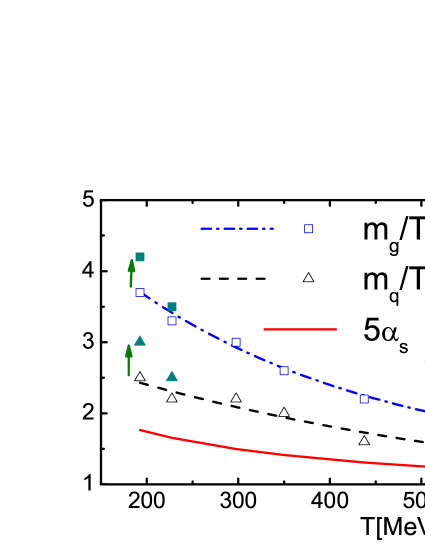
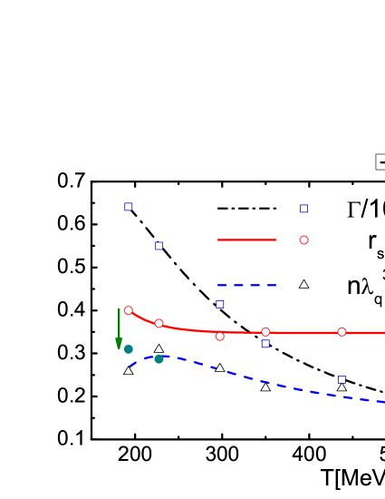
Figure 1: Left panel:Temperature dependences of the model input quantities: the coupling constant $\alpha_{s}$ (scaled by 5) and quasiparticle mass-to-temperature ratio ($m_{q}=m_{\bar{q}}$). Right panel: Temperature dependences of the calculated interparticle average distance $r_{s}$ (Wigner-Seitz radius), the quark quasiparticles degeneracy parameter $\chi$ and the plasma coupling parameter $\Gamma$. Lines are smooth interpolation between the CPIMC points. To ilustrate sensibility of this model to input data the green solid symbols and arrows show changes of the CPIMC average interparticle distance (right panel) related to the quasiparticle mass variation on left panel.

In the studied temperature range, $190\text{ MeV}<T<600\text{ MeV}$, the QGP is, in fact, quantum degenerate, since the degeneracy parameter $\chi=n_{q}\lambda_{q}^{3}$ (where the thermal wave length $\lambda_{q}$ was defined in the previous sect.) varies from $\sim 20$ to $\sim 8$, see Fig. 1 (right panel). The degeneracy parameters for different species does not coincide, since the quasiparticle masses are different.

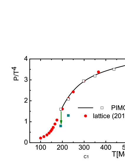
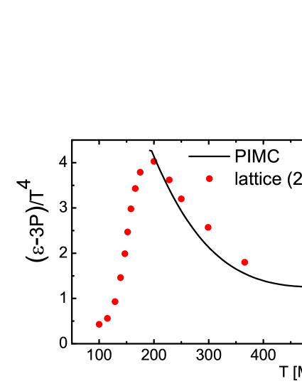
Figure 2: Equation of state (left panel) of the QGP from CPIMC simulations (open squares). The solid line is a smooth interpolation between the CPIMC points. The solid symbols illustrate the changes in equation of state for presented by Fig. 1 quasiparticle mass variation. Trace anomaly (right panel) of the QGP from CPIMC simulations is presented by solid line. Both CPIMC results are compared to lattice data of Fodor09 ; Csikor:2004ik

As follows from analysis of Fig. 1 and Fig. 2 this model is highly sensitive to quasiparticle mass variations. This allow to fit lattice EOS and to choose optimal values of gluon and quark masses in order to proceed in predictions of other properties concerning the internal structure and in the future also non-equilibrium dynamics of the QGP. High sensitivity of EOS to mass variation adds to background of this procedure. Let us also note that increase of quasiparticles masses reduces the influence of quantum effects, so high sensitivity of EOS to masses proved the importance of quantum effects at these temperatures. Figure 2 presents also the trace anomaly ($(\varepsilon-3P)/T^{4}$) calculated as related combination of derivatives of equation of state. In order to avoid the numeric noise, the derivatives of a smooth interpolation between the CPIMC points of equation of state (Fig. 2) were taken. The CPIMC results are compared to lattice data of Fodor09 ; Csikor:2004ik . It is not surprising that agreement with the lattice data for trace anomaly is also good, since it is a direct consequence of the good reproduction of the pressure.

Let us now consider the spatial arrangement of the quasiparticles in the QGP by studying the pair distribution functions (PDF) $g_{ab}(R)$. They give the probability density to find a pair of particles of types $a$ and $b$ at a certain distance $R=|R_{1}-R_{2}|$ from each other and are defined, for example, in canonical ensemble as

$$g_{ab}(|R_{1}-R_{2}|)=\frac{1}{Z\left(N,V,\beta\right)\text{,}}\sum_{\sigma}\int\limits_{V}dr\;dQ,\delta(R_{1}-r^{a}_{1})\delta(R_{2}-r^{b}_{2})\;\rho(r,Q,\sigma;N_{u},N_{d},N_{s},\bar{N}_{u},\bar{N}_{d},\bar{N}_{s},N_{g};\beta),$$ (9)

The PDF depend only on the difference of coordinates because of the translational invariance of the system. In a non-interacting classical system, $g_{ab}(R)\equiv 1$, whereas interactions and quantum statistics result in a re-distribution of the particles. At temperatures $T=193\text{ MeV}$ the PDF averaged over the quasiparticle spin, colors and flavors are shown in the panels of Fig. 3.

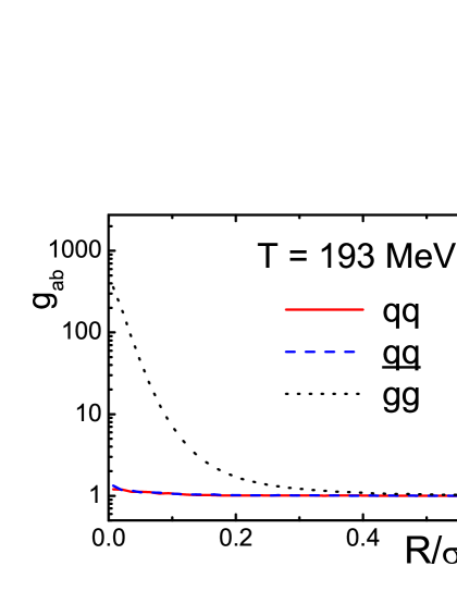
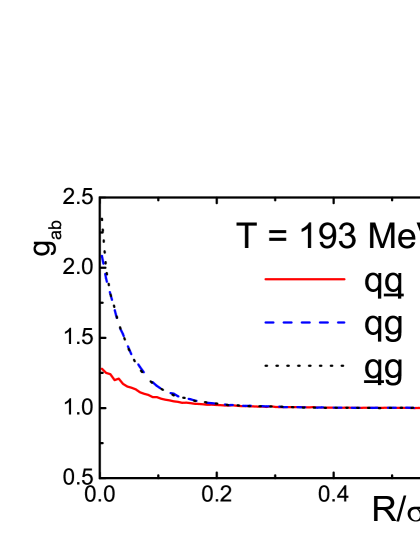
Figure 3: Pair distribution functions of identical (left panel) and different (right panel) quasiparticles at temperature $T=193\text{ MeV}$. The distance is measured in units of $\sigma=1.1$ fm.

At distances, $R/\sigma\geq r_{s}(r_{s}\approx 0.35)$ all PDF are practically equal to unity (Fig. 3) like in ideal gas due to the ’Debye’ screening of the color Coulomb interaction. A drastic difference in the behavior of the PDF of quarks and gluons (the anti-quark PDF is identical to the quark PDF) occurs at distances $R/\sigma\leq r_{s}$. Very well pronounced is the short-range structure of nearest neighbors. Here the gluon-gluon and gluon-quark PDF increases monotonically when the distance goes to zero. Behavior of these PDF is a clear manifestation of an effective pair attraction. Attraction suggests that the color vectors of nearest neighbor quasiparticles are anti-parallel. The QGP lowers its total energy by minimizing the color Coulomb interaction energy via a spontaneous “anti-ferromagnetic” ordering of color vectors. From physical point of view this means formation of the gluon-gluon and gluon-(anti)quark clusters, which are more or less uniformly distributed in space. The last conclusion comes from the fact that the (anti)quark-(anti)quarks PDF are close to unity. Oscillations of the PDF at very small distances of order $R\leq 0.1\sigma$ are related to Monte Carlo statistical error, as probability of quasiparticles being at short distances quickly decreases.

The main physical reason for arising the well separated from each other the gluon-gluon and gluon-(anti)quark) quasiparticle clusters is the consequence of the great difference in values of quadratic Casimir invariants $q_{2}=<Q_{i}^{(l)}|Q_{i}^{(l)}>$ for gluon-gluon $q_{2}=24$, (anti)quark-(anti)quark $q_{2}=4$ and gluon-(anti)quark $q_{2}=\sqrt{24*4}\approx 10$ in color Kelbg (Coulomb) potentials of quasiparticles interactions .

The second physical reason of the PDF difference is spatial quantum uncertainty and different property of Bose and Fermi statistics of gluon and (anti)quark quasiparticles. Fermi statistics results in effective quark-quark and aniquark-antiquark repulsion, while Bose one results to effective qluon-qluon attraction. More strong interaction of the QGP quasiparticles with gluons than with quarks is also consequence of the gluon better localization in comparison with quarks. As we mentioned before uncertainity in particle localization is defined by the ratio $1/m$. Localization is better for heavier gluon quasipartcles. To verify the relevance of all these trends, a more refined color, flavor, and spin-resolved analysis of the PDF is necessary, together with simulations in a broader range of temperatures which are presently in progress.

Details of our path integral Monte-Carlo simulations have been discussed elsewhere in a variety of papers and review articles, see, e.g. zamalin ; rinton and references therein. The main idea of the simulations consists in constructing a Markov chain of quasiparticle configurations. Additionally to the case of electrodynamic plasmas here we randomly sample the color quasiparticle variables $Q$ according to the group SU(3) Haar measure.

IV Conclusion

Color quantum Monte Carlo simulations based on the quasiparticle model of the QGP are able to reproduce the lattice equation of state and other thermodynamic functions (even near the critical temperature) and also yield valuable insight into the internal structure of the QGP. Our results indicate that the QGP reveals quasiparticle clustering and liquid-like (rather than gas-like) properties even at the highest considered temperature.

For our simulations we have introduced new relativistic path integral measure and have developed procedure of sampling color quasiparticle variables according to the group SU(3) Haar measure with the quadratic and cubic Casimir conditions. Our analysis is still simplified and incomplete. It is still confined only to the case of zero baryon chemical potential. The input of the model also requires refinement. Work on these problems is in progress.

We acknowledge stimulating discussions with Prof. P. Levai, D. Blaschke, R. Bock, and H. Stoecker.

References

- (1) E. Shuryak, Prog. Part. Nucl. Phys. 62, 48 (2009).
- (2) Z. Fodor and S. D. Katz, arXiv:0908.3341 [hep-ph].
- (3) S. Borsanyi, G. Endrodi, Z. Fodor, A. Jakovac, S. D. Katz, S. Krieg, C. Ratti, K. K. Szabo, JHEP 1011:077,2010
- (4) P. Hartmann, Z. Donko, P. Levai, G.J. Kalman, J. Phys. A42, 214029 (2006); Nucl. Phys. A774, 881-884, (2006);
- (5) D. F. Litim and C. Manuel, Phys. Rev. Lett. 82, 4981 (1999); Nucl.Phys. B 562, 237 (1999); Phys. Rev. D 61, 125004 (2000); Phys. Rep. 364, 451 (2002),
- (6) M. Laine and C. Manuel, Phys. Rev. D 65, 077902 (2002),
- (7) C. Manuel and S. Mrowczynski, Phys. Rev. D 68, 094010 (2003),
- (8) P. F. Kelly, Q. Liu, C. Lucchesi and C. Manuel, Phys. Rev. D 50, 4209 (1994)
- (9) M. Hofmann, M. Bleicher, S. Scherer, et al., Phys. Lett. B 478, 161 (2000).
- (10) B. A. Gelman, E. V. Shuryak, and I. Zahed, Phys. Rev. C 74, 044908 (2006); 74, 044909 (2006).
- (11) S. Cho and I. Zahed, Phys. Rev. C 79, 044911 (2009); Phys. Rev. C 80, 014906 (2009); arXiv:0910.2666 [nucl-th]; arXiv:0910.1548 [nucl-th]; arXiv:0909.4725 [nucl-th]; K. Dusling and I. Zahed, Nucl. Phys. A 833, 172 (2010).
- (12) M.H. Thoma, IEEE Trans. Plasma Science 32, 738 (2004)
- (13) A. Filinov, M. Bonitz, and W. Ebeling, J. Phys. A 36, 5957 (2003).
- (14) G. Kelbg, Ann. Phys. (Leipzig) 12, 219 (1962); 13, 354 (1963).
- (15) K. Dusling and C. Young, arXiv:0707.2068 [nucl-th].
- (16) V.S. Filinov, M. Bonitz, Yu. B. Ivanov, et al., Contrib. Plasma Phys., 49, 536 (2009).
- (17) V.S. Filinov, M. Bonitz, Yu. B. Ivanov, et al., e-Print: arXiv:1006.3390 [nucl-th].
- (18) V. S. Filinov, M. Bonitz, Y.B. Ivanov, V.V. et al. Contrib. Plasma. Phys. 51, N4, 322-327 (2011).
- (19) P. Petreczky, F. Karsch, E. Laermann, et al., Nucl. Phys. Proc. Suppl. 106, 513 (2002).
- (20) J. Liao and E. V. Shuryak, Phys. Rev. D 73, 014509 (2006).
- (21) S. K. Wong, Nuovo Cimento A 65, 689 (1970).
- (22) R. P. Feynman, and A. R. Hibbs, Quantum Mechanics and Path Integrals (McGraw-Hill, New York, 1965).
- (23) V. M. Zamalin, G. E. Norman, and V. S. Filinov, The Monte Carlo Method in Statistical Thermodynamics (Nauka, Moscow, 1977), (in Russian).
- (24) V. S. Filinov, M. Bonitz, W. Ebeling, and V. E. Fortov, Plasma Phys. Control. Fusion 43, 743 (2001).
- (25) G. M. Prosperi, M. Raciti, and C. Simolo, Prog. Part. Nucl. Phys. 58, 387 (2007).
- (26) A. V. Filinov, V. S. Filinov, Yu. E. Lozovik and M. Bonitz, Introduction to Computational Methods for Many-Body Physics, Ed. by M. Bonitz and D. Semkat (Rinton Press, Princeton, 2006).