Kalb-Ramond excitations in a thick-brane scenario with dilaton

Abstract

We compute the full spectrum and eigenstates of the Kalb-Ramond field in a warped non-compact Randall-Sundrum -type five-dimensional spacetime in which the ordinary four-dimensional braneworld is represented by a sine-Gordon soliton. This 3-brane solution is fully consistent with both the warped gravitational field and bulk dilaton configurations. In such a background we embed a bulk antisymmetric tensor field and obtain, after reduction, an infinite tower of normalizable Kaluza-Klein massive components along with a zero-mode. The low lying mass eigenstates of the Kalb-Ramond field may be related to the axion pseudoscalar. This yields phenomenological implications on the space of parameters, particularly on the dilaton coupling constant. Both analytical and numerical results are given.

1 Introduction

Field theoretic scenarios derived from string theory bring necessarily together the standard model degrees of freedom and the gravitational field to interact in some higher dimensional bulk space-time.

Extra dimensions have shown to be instrumental for solving fundamental problems such as the hierarchy gap between the gravitational and the gauge coupling scales leading to de Sitter (or de Sitter-like) geometries in four dimensions RS .

Regarding standard gauge interactions, it is known that the electroweak excitations are deposited on D-branes by the open strings ending on them polchinski . Thus, normalized standard model gauge modes are expected to be localized on topological defects of lower dimensionality representing p-branes in a low energy setup keha-tamva ; cunhachris . On the same token, fermion fields have also been found to be localized on the brane, as expected (see e.g. fermions ).

Besides the standard model fields and particles a series of entities not yet discovered are the expected residuals left in quantum field theories emerging from a low energy string inception. Among these the dilaton is a scalar field inevitably present along with the graviton. Moreover, when gravitation is recovered from string theory, an antisymmetric tensor appears together with graviton and dilaton in the Neveu-Schwarz bosonic sector of the low energy string effective action ashoke . Therefore, to start, we will be concerned with the low energy interaction of these three fields plus a topological scalar representing our 3-brane world.

Motivations to consider the Kalb-Ramond field KR in a thick braneworld scenario are actually many. It is known that since the graviton is a massless closed string excitation it can naturally propagate at will across the whole space polchinski . But then, one should also consider in the bulk other fields related to closed strings. Two such degrees of freedom are the above mentioned scalar dilaton and a second-rank antisymmetric tensor usually met in supergravity theories superspace . In extended supergravity this tensor, associated with the Kalb-Ramond field, becomes a factual component of the supergravity multiplet. Since massless modes are expected to be the most relevant in the ordinary world, this sector of the low energy string theory is likely responsible for most observable effects in cosmic phenomena GSW strings . Although not a standard model component, the KR field has been argued to be localized on the brane much in a similar way as the U(1) vector gauge field in CHRISTIANSEN ; localized tensor .

In the last decade, the KR field has been related to torsion, a geometric property of spacetime (such as curvature) that modifies the electromagnetic field strength through the affine connection in the covariant derivative. Using a generalized form of the Einstein-Cartan (EC) action, it has been shown indianos 99 that the third-rank field-strength tensor of the KR field, $H_{\mu\nu\rho}$, can be directly identified with torsion to guarantee gauge symmetry. Interestingly, a parity violating term appears naturally if one considers a pseudotensorial extension of the affine connection. Such a parity breaking gravitational interaction emerges not only from a theoretical viewpoint but also from observation. For example, in indianos neutrino it has been shown that a parity violating gravitation can flip the helicity of fermions providing a possible explanation to this neutrino problem. Likewise, the anisotropy in the cosmic microwave background radiation might be explained by a parity violating coupling of the electromagnetic field with a pseudoscalar CMB , presumably the so-called axion. Indeed the dual scalar of the pseudotensor component of the connection discussed above can be identified with that particle.

It is worth mentioning that a completely antisymmetric torsion, as provided by the KR field, can induce parity violation only in the matter (spin 1/2) sector but not in the curvature or $U(1)$ gauge sector. This is traced to the fact that such a tensor can always be expressed in terms of its dual field, the axion $\chi$, defined through the duality relation $H_{\mu\nu\rho}=\epsilon_{\mu\nu\rho\sigma}\partial^{\sigma}\chi$ (the solution for $\chi$ in flat space is linear in the comoving time) indianos EPJ 2002 . See axion KR for early work relating the axion and the KR field (see also axion dilaton ).

In face of the above prospect, in the present paper we will assume a massless five-dimensional KR field along with gravity. However, since the breakdown of supersymmetry may result in the generation of mass for the axion, we will also consider a Kaluza-Klein mechanism to endow the KR field with mass in ordinary space. In this respect, it has been shown that dimensionally reduced $U(1)$ gauge fields are not normalizable unless the effective coupling is modified by the dilaton youm1 so we shall dynamically include the massless dilaton in the curved background defined for the KR field. In other words, both brane and dilaton configurations will be geometrically consistent solutions of a two scalar world action in a warped 5D spacetime. These configurations arise as topological kinks of a sine-Gordon type potential function.

The paper is organized as follows. The framework is presented in the next section. In Sect. 3 we study the five-dimensional equations of motion for the KR field and discuss a few cases from a quantum-mechanical analog point of view. Next, in Sect. 4 we cope with the general problem and compute spectra and eigenfunctions for generic values of the parameters. In Sect. 5 we draw our conclusions.

2 The model

We consider a 5D action where a bulk Kalb-Ramond field, $B_{NP}$, is coupled to the dilaton, $\Pi$, in a warped space-time defined by two metric functions ($\Lambda$ and $\Sigma$) and a brane field $\Phi$:

$$S=\int d^{4}x\,dy\,\sqrt{G}\ \left\{2M^{3}R_{(5)}-\frac{1}{2}(\partial\Phi)^{2}-\frac{1}{2}(\partial\Pi)^{2}\right.$$

$$\left.-\mathcal{V}(\Phi,\Pi)+\dfrac{1}{12}\,e^{-\lambda\Pi}H_{MNP}H^{MNP}\right\}.$$ (1)

The tensor gauge field-strength is $H_{MNP}=\partial_{M}B_{NP}+\partial_{P}B_{MN}+\partial_{N}B_{PM}$, $R_{(5)}$ is the Ricci scalar, and $M$ is the Planck mass in the bulk. As usual, we employ Latin capitals in 5D and Greek lower case letters in the four-dimensional slice. We adopt the following ansatz for the metric

$$ds^{2}=G_{\mu\nu}dx^{\mu}dx^{\nu}+e^{2\Sigma(y)}dy^{2},$$ (2)

where $G_{\mu\nu}=e^{2\Lambda(y)}\eta_{\mu\nu}$ and diag$(\eta)=(-1,1,1,1)$; $G=-\det G_{MN}$. We will assume that all the scalar fields depend just on the fifth coordinate, $y$ keha-tamva .

Considering the scalars back reaction on the metric, the equations of motion for $\Pi$, $\Phi$, $\Lambda$ and $\Sigma$ are

$$\frac{1}{2}(\Phi^{\prime})^{2}+\frac{1}{2}(\Pi^{\prime})^{2}-e^{2\Sigma(y)}\mathcal{V}(\Phi,\Pi)=24M^{3}(\Lambda^{\prime})^{2},$$

$$\frac{1}{2}(\Phi^{\prime})^{2}+\frac{1}{2}(\Pi^{\prime})^{2}+e^{2\Sigma(y)}\mathcal{V}(\Phi,\Pi)=-12M^{3}\Lambda^{\prime\prime}$$

$$-24M^{3}(\Lambda^{\prime})^{2}+12M^{3}\Lambda^{\prime}\Sigma^{\prime},$$ (3)

and

$$\Phi^{\prime\prime}+(4\Lambda^{\prime}-\Sigma^{\prime})\Phi^{\prime}=e^{2\Sigma}\ \frac{\partial\mathcal{V}}{\partial\Phi},$$

$$\Pi^{\prime\prime}+(4\Lambda^{\prime}-\Sigma^{\prime})\Pi^{\prime}=e^{2\Sigma}\ \frac{\partial\mathcal{V}}{\partial\Pi}.$$ (4)

where the prime means derivative with respect to $y$.

The potential functional $\mathcal{{V}}(\Phi,\Pi)$ stems from a supergravity motivated definition supergravity which can be applied to non-supersymmetric systems. Based on a standard sine-Gordon potential, the functional $V(\Phi)=b^{-2}\ (1-\cos(b\,\Phi))$ gets deformed in order to include the effects of the warped metric and the dilaton. The final expression

$$\mathcal{{V}}(\Phi,\Pi)=e^{({\Pi}/{\sqrt{12M^{3}}})} \left(\frac{2}{b^{2}}\sin^{2}(\frac{b}{2}\,\Phi+\frac{\pi}{2})-\right.$$ (5)

$$\left.\frac{5}{2M^{3}b^{4}}\cos^{2}(\frac{b}{2}\,\Phi+\frac{\pi}{2})\right),$$

is found after some algebra by looking for the consistency of the equations of motion (3) and (4) CHRISTIANSEN and symmetrizing the bounce eq.(6) with respect to $y=0$. The solutions to the equations for $\Phi$ and $\Pi$ represent the braneworld and the dilaton final configurations respectively. They are consistent altogether with the metric functions $\Lambda$ and $\Sigma$. Indeed, the following solution, interpolating vacua and kinking on our 4D-world slice

$$\Phi=\frac{4}{b}\ (\arctan\ e^{y}-\frac{\pi}{4})$$ (6)

is compatible with a dilaton configuration

$$\Pi=\frac{1}{\sqrt{3M^{3}}b^{2}}\ln\cosh y,$$ (7)

in a gravitational field given by

$$\Lambda=-\frac{1}{{3M^{3}}b^{2}}\ln\cosh y,$$ (8)

and

$$\Sigma=-\frac{1}{{12M^{3}}b^{2}}\ln\cosh y.$$ (9)

With this set of solutions the scalar action is finite provided $\lambda$ is above a critical value $\lambda_{0}=-{17}/{4\sqrt{3M^{3}}}$ CHRISTIANSEN . By means of the warping functions (8) and (9), the effective four-dimensional Planck scale can be defined by

$$M_{P}^{2} = M^{3}\int_{-\infty}^{\infty}dy\ e^{4\Lambda(y)+\Sigma(y)}$$ (10)

$$= M^{3}\int_{-\infty}^{\infty}dy\ (\operatorname{sech}y)^{{C}/{M^{3}}}$$

where $C=17/12b^{2}$. After integration, we obtain a (finite) close expression for the effective Planck scale as a function of the 5D Planck scale

$$M_{P}^{2}=M^{3}\,\frac{\sqrt{\pi}\,\,\Gamma\!\left(\frac{C}{2M^{3}}\right)}{\Gamma\!\left(\frac{1}{2}+\frac{C}{2M^{3}}\right)}.$$ (11)

By studying the fluctuations of the metric about the background configuration, eqs.(6)-(9), it is possible to see that this model supports a normalizable massless graviton (zero-mode of the gravitational field) localized on the membrane keha-tamva .

3 Field equations of the KR field

Since the axion field is supposed to be extremely diluted in space it is likely that the Kalb-Ramond field would not contribute significantly to the geometrical background. Indeed, in a Randall-Sundrum scenario it has been explicitly shown that the Kalb-Ramond energy density has only a tiny value $\sim 10^{-62}$ KR RS . Thus, we can safely study the behavior of propagating modes in the topological background configuration above found.

The equations of motion for $B_{MN}$ in the bulk are given by

$$\frac{1}{\sqrt{G}}\,\partial_{M}(G^{MR}G^{NS}G^{PQ}H_{RSQ}\sqrt{G}e^{-\lambda\Pi(y)})=0.$$ (12)

In order to solve these equations, we adopt the following gauge choices

$$B^{\mu 5}=0,\ \partial_{\mu}B^{\mu\nu}=0.$$ (13)

Next, we perform the usual Kaluza-Klein decomposition as follows

$$B^{\mu\nu}(x,y)=\sum_{n}\,b_{n}^{\mu\nu}(x)w_{n}(y)$$ (14)

yielding

$$\left[\Box+\left(\frac{1}{w_{n}\ g}\partial_{5}(g\partial^{5}w_{n})\right)\right]\ b_{n}^{\mu\nu}=0$$ (15)

with $g(y)=e^{4\Lambda+\Sigma}\exp[-\lambda\Pi]$. The Kaluza-Klein spectrum of the Kalb-Ramond field is then given by

$$[g^{-1}\partial_{5}g\partial^{5}+m_{n}^{2}]\ w_{n}=0,$$ (16)

where $m_{n}^{2}$ is the 4D squared boson mass of the tensor field $n$th-mode, satisfying $p_{n}^{2}=-m_{n}^{2}$. Operating further, the $y$-dependent equation reads

$${6M^{3}b^{2}}w_{n}^{\prime\prime}(y)-{(15/2+2\lambda\sqrt{3M^{3}})}\tanh y\ w_{n}^{\prime}(y)+$$

$$m_{n}^{2}{6M^{3}b^{2}}\operatorname{sech}^{1/6M^{3}b^{2}}y\ w_{n}(y)=0,$$ (17)

where the prime means $\partial/\partial y$.

In contrast to Ref. CHRISTIANSEN , here we adopt a different relation between the fundamental parameters $M$ and $b$ in order to analyze a new equation of motion for the gauge field. Now, the last term of eq.(17) involves the function $\operatorname{sech}^{6}y$ instead of $\operatorname{sech}^{2}y$ that was considered in CHRISTIANSEN . This, together with a different constant factor in the two last terms, imposes the necessity of solving a new differential equation which brings about different spectra and the eigenfunctions associated.

With the choice $36M^{3}\,b^{2}=1$ eq.(17) can be written as

$$w_{n}^{\prime\prime}(y)+\tilde{c}\tanh y\ w_{n}^{\prime}(y)+m_{n}^{2}\operatorname{sech}^{6}y\ w_{n}(y)=0,$$ (18)

where $\tilde{c}=-3(15+4\lambda\sqrt{3M^{3}})$. For simplicity, we drop the subindexes of the propagation modes in what follows. We will solve this equation exactly in what follows.

3.1 Special cases

By means of the transformation

$$w(y)=e^{-\alpha\Lambda}\,W(z),\ \ \ \frac{dz}{dy}=e^{\Lambda/4}$$ (19)

we can turn eq.(17) into

$$\left[-\frac{d^{2}}{dz^{2}}+\mathfrak{V}(z)\right]W(z)=m^{2}W(z),$$ (20)

where $\mathfrak{V}(z)={\alpha}\,e^{-\Lambda/2}(\Lambda^{\prime\prime}+({\alpha}-\frac{1}{4})\ \Lambda^{\prime}{\leavevmode\nobreak\ }^{2})$ and $\alpha=2+\lambda\sqrt{3M^{3}}/2$, which is a Schrodinger-like equation in the variable $z\in(-1,1)$ (see e.g. RS ; keha-tamva ).

In the present case we obtain

$$z(y)=\arctan(\tanh\frac{y}{2})+\frac{1}{2}\operatorname{sech}\!y\tanh\!y,$$ (21)

$$w(y)=\cosh^{\gamma}\!y\,W(z),$$ (22)

and

$$\mathfrak{V}(z(y))=-\gamma\cosh^{4}\!y\left[1+(3-\gamma)\sinh^{2}\!y\right],$$ (23)

where $\gamma=12\,\alpha$ and $\tilde{c}=3-2\gamma$. Both the change of variables (21), (22) and the potential function (23) are completely different from those in CHRISTIANSEN . In the present case the solution is more difficult, but although we cannot analytically invert eq.(21), we can do it numerically and compute $\mathfrak{V}(y(z))$ for several values of $\gamma$, see Fig.1.

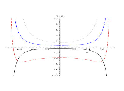
Figure 1: Potential $\mathfrak{V}(z)$ numerically computed for some values of the parameters: $\gamma=1/2$ (solid black line), $\gamma=30/8$ (dashed red line), $\gamma=-1/2$ (long-dashed blue line), and $\gamma_{0}=-3/2$ (dot-dashed grey line), corresponding to critical $\lambda_{0}$. Note the divergency at $z\rightarrow\pm\pi/4$.

3.1.1 The case $\gamma$=0 ($\tilde{c}=3$)

In this case, the potential function (23) seems trivial, but in fact, for $z=\pm\pi/4$ we have $y\rightarrow\pm\infty$ and therefore solutions to eq. (20) must be null in $|z|\geq\pi/4$. The potential in $z$ thus corresponds to an infinite square-well of width $\pi/2$. The normalized solutions of the Schrodinger equation (20) can be analytically obtained

$$W(z)=\frac{2}{\sqrt{\pi}}\cos((4n+2)\ z)+\frac{2}{\sqrt{\pi}}\sin(4n\ z).$$ (24)

Here, the mass spectrum is given by $m=2(n+1)$ where the parity of $n$ is the parity of the associated solution. In the actual $y$ space these solutions read

$$w^{(1)}(y)=\frac{2b_{1}}{\sqrt{\pi}}\cos((4n+2)(\arctan(\tanh\,\frac{y}{2})\leavevmode\nobreak\ \leavevmode\nobreak\ \leavevmode\nobreak\ \leavevmode\nobreak\ \leavevmode\nobreak\ \leavevmode\nobreak\ \leavevmode\nobreak\ \leavevmode\nobreak\ \leavevmode\nobreak\ \leavevmode\nobreak\$$

$$+\frac{1}{2}\operatorname{sech}\,y\tanh\,y))\leavevmode\nobreak\ \leavevmode\nobreak\ \leavevmode\nobreak\$$ (25)

and

$$w^{(2)}(y)=\frac{2b_{2}}{\sqrt{\pi}}\sin(4n\arctan(\tanh\,\frac{y}{2})\leavevmode\nobreak\ \leavevmode\nobreak\ \leavevmode\nobreak\ \leavevmode\nobreak\ \leavevmode\nobreak\ \leavevmode\nobreak\ \leavevmode\nobreak\ \leavevmode\nobreak\ \leavevmode\nobreak\ \leavevmode\nobreak\ \leavevmode\nobreak\ \leavevmode\nobreak\ \leavevmode\nobreak\ \leavevmode\nobreak\ \leavevmode\nobreak\ \leavevmode\nobreak\ \leavevmode\nobreak\$$

$$+\frac{1}{2}\operatorname{sech}\,y\tanh\,y)).\leavevmode\nobreak\$$ (26)

where $b_{1},b_{2}$ are normalization constants. Solutions (25) and (26) for the first values of the spectrum are shown in Figs. 3 and 3 respectively.

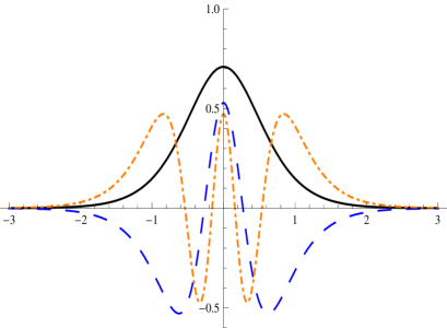
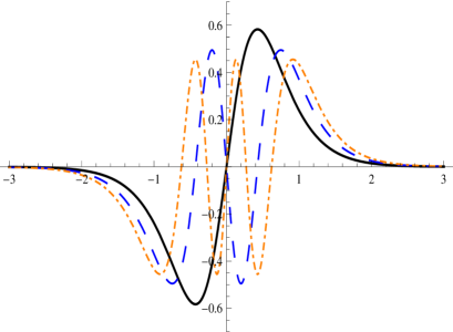
Figure 2: First normalized symmetric solutions, Eq. (25), for $\tilde{c}=3$: $m=2$ (solid black line), $m=6$ (dashed blue line), $m=10$ (dot-dashed orange line). (Color figure online)

Figure 3: First normalized antisymmetric solutions, Eq. (26), for $\tilde{c}=3$: $m=4$ (solid black line), $m=8$ (dashed blue line), $m=12$ (dot-dashed orange line). (Color figure online)

3.1.2 The $\gamma$=1/2, ($\tilde{c}=2$) case

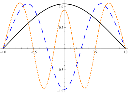
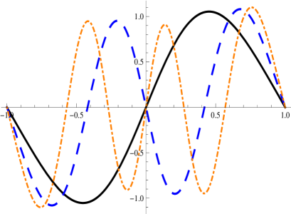
Figure 4: Symmetric solutions Eq. (33) for $\tilde{c}=2$: $m=1.68159532$ (solid black line), $m=5.66985735$ (dashed blue line), $m=9.66824247$ (dot-dashed orange line). (Color figure online)

Figure 5: Antisymmetric solutions Eq. (33) for $\tilde{c}=2$: $m=3.67229037$ (solid black line), $m=7.668808762$ (dashed blue line), $m=11.667894313$ (dot-dashed orange line). (Color figure online)

By means of the following transformation

$${x}=\sqrt{m}\tanh(y)$$ (27)

we can rewrite eq. (18) as

$$w^{\prime\prime}(x)+(\tilde{c}-2)\frac{x}{m-x^{2}}w^{\prime}(x)+(m-x^{2})w(x)=0.$$ (28)

Now, with $\tilde{c}=2$ we get

$$-w^{\prime\prime}({x})+{x}^{2}w({x})=m\ w({x})$$ (29)

This is the equation of motion of a nonrelativistic quantum particle of energy $m$ in a harmonic potential $V({x})={x}^{2}$ for $-\sqrt{m}<{x}<\sqrt{m}\$ ($V({x})=\infty$ for $|{x}|\geq\sqrt{m}$ and thus $w({x})=0$ in this region).

With $x\rightarrow\frac{x}{\sqrt{2}}$, it reads as a standard parabolic cylinder differential equation

$$w^{\prime\prime}({x})+(-\frac{x^{2}}{4}+\frac{m}{2})\,w({x})=0$$ (30)

with analytical even and odd solutions given by

$$w_{1}(x)=e^{-x^{2}/4}\ _{1}F_{1}(-\frac{m}{4}+\frac{1}{4};\frac{1}{2};\frac{x^{2}}{2}),$$

$$w_{2}(x)=xe^{-x^{2}/4}\ _{1}F_{1}(-\frac{m}{4}+\frac{3}{4};\frac{3}{2};\frac{x^{2}}{2}),$$ (31)

ABRAMOWITZ where ${}_{1}F_{1}$ are confluent hypergeometric functions.

The solution can also be written in terms of parabolic cylinder functions

$$D_{\nu}(x)=\frac{2^{\nu/2}\sqrt{\pi}}{\Gamma(\frac{1-\nu}{2})}\left[1-\frac{1}{2}\,(1+2\nu)\,\frac{x^{2}}{2!}+\frac{1}{4}\,(3+4\nu+4\nu^{2})\,\frac{x^{4}}{4!}\right.$$

$$\left.-\frac{1}{8}\,(15+34\nu+12\nu^{2}+8\nu^{3})\,\frac{x^{6}}{6!}+\mathcal{O}(x^{8})\right]$$

$$-\frac{2^{\frac{\nu+1}{2}}\sqrt{\pi}}{\Gamma(-\frac{\nu}{2})}\left[x-\frac{1}{2}\,(1+2\nu)\,\frac{x^{3}}{3!}+\frac{1}{4}\,(7+4\nu+4\nu^{2})\,\frac{x^{5}}{5!}\right.$$

$$-\left.\frac{1}{8}\,(27+58\nu+12\nu^{2}+8\nu^{3})\,\frac{x^{7}}{7!}+\mathcal{O}(x^{9})\right]$$ (32)

as

$$w(\tilde{x})=A_{1}\ D_{\frac{m-1}{2}}(\sqrt{2m}\leavevmode\nobreak\ \tilde{x})+A_{2}\ D_{\frac{m-1}{2}}(-\sqrt{2m}\,\tilde{x}),$$ (33)

where $A_{1}=A_{2}=A/\sqrt{2}$ for symmetric solutions and $A_{1}=-A_{2}=A$ for the anti-symmetric ones. Here, $\tilde{x}=x/\sqrt{2m}$. For simplicity, the value of the normalization constant can be approximated by $A\simeq 1/\sqrt{((m-m_{0})/2)!}$, where $m_{0}=1.556$ for even solutions and $m_{0}=1.581$ for odd solutions. The mass eigenvalues can also be well approximated by $m\simeq 2n+5/3$, with $n\in\mathbb{N}$, see Figs. 5 and 5.

In terms of $y$, solutions (33) read

$$w^{(1)}(y)=c_{1}\frac{A}{\sqrt{2}}\left[D_{\frac{m-1}{2}}(\sqrt{2m}\leavevmode\nobreak\ \tanh(y))\leavevmode\nobreak\ \leavevmode\nobreak\ \leavevmode\nobreak\ \leavevmode\nobreak\ \leavevmode\nobreak\ \leavevmode\nobreak\ \leavevmode\nobreak\ \leavevmode\nobreak\ \leavevmode\nobreak\ \leavevmode\nobreak\ \leavevmode\nobreak\ \leavevmode\nobreak\ \leavevmode\nobreak\ \leavevmode\nobreak\ \leavevmode\nobreak\ \leavevmode\nobreak\ \leavevmode\nobreak\ \leavevmode\nobreak\ \leavevmode\nobreak\ \leavevmode\nobreak\ \leavevmode\nobreak\ \right.$$

$$\left.+D_{\frac{m-1}{2}}(-\sqrt{2m}\,\tanh(y))\right]\leavevmode\nobreak\ \leavevmode\nobreak\ \leavevmode\nobreak\ \leavevmode\nobreak\$$ (34)

$$w^{(2)}(y)=c_{2}A\left[D_{\frac{m-1}{2}}(\sqrt{2m}\leavevmode\nobreak\ \tanh(y))\leavevmode\nobreak\ \leavevmode\nobreak\ \leavevmode\nobreak\ \leavevmode\nobreak\ \leavevmode\nobreak\ \leavevmode\nobreak\ \leavevmode\nobreak\ \leavevmode\nobreak\ \leavevmode\nobreak\ \leavevmode\nobreak\ \leavevmode\nobreak\ \leavevmode\nobreak\ \leavevmode\nobreak\ \leavevmode\nobreak\ \leavevmode\nobreak\ \leavevmode\nobreak\ \leavevmode\nobreak\ \right.$$

$$\left.-D_{\frac{m-1}{2}}(-\sqrt{2m}\,\tanh(y))\right].$$ (35)

where $c_{1},c_{2}$ are new normalization constants. See Figs. 7 and 7.

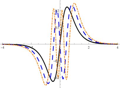
Figure 6: Symmetric solutions $w^{(1)}(y)$, Eq. (34), for $\tilde{c}=2$: $m=1.68159532$ (solid black line), $m=5.66985735$ (dashed blue line), $m=9.66824247$ (dot-dashed orange line). (Color figure online)

Figure 7: Antisymmetric solutions $w^{(2)}(y)$, Eq. (35), for $\tilde{c}=2$: $m=3.67229037$ (solid black line), $m=7.668808762$ (dashed blue line), $m=11.667894313$ (dot-dashed orange line). (Color figure online)

Looking at eq.(23), cases like $\gamma=3$ and $\gamma=2$ result in simple forms of $\mathfrak{V}(z(y))$ seemingly affordable. However these do not bring about exact solutions in the Schrodinger approach because such expressions cannot be analytically inverted in terms of $z$ (see eq.21).

4 The general solution

In order to obtain the general solution to Eq. (18) we perform the following transformation

$$z=\tanh^{2}\!y.$$ (36)

Now, Eq. (18) becomes

$$w^{\prime\prime}(z)+\left(\frac{1/2}{z}+\frac{1-\tilde{c}/2}{z-1}\right)w^{\prime}(z)\leavevmode\nobreak\ \leavevmode\nobreak\ \leavevmode\nobreak\ \leavevmode\nobreak\ \leavevmode\nobreak\ \leavevmode\nobreak\ \leavevmode\nobreak\ \leavevmode\nobreak\ \leavevmode\nobreak\ \leavevmode\nobreak\ \leavevmode\nobreak\ \leavevmode\nobreak\ \leavevmode\nobreak\ \leavevmode\nobreak\ \leavevmode\nobreak\ \leavevmode\nobreak\ \leavevmode\nobreak\ \leavevmode\nobreak\ \leavevmode\nobreak\ \leavevmode\nobreak\ \leavevmode\nobreak\ \leavevmode\nobreak\ \leavevmode\nobreak\ \leavevmode\nobreak\ \leavevmode\nobreak\ \leavevmode\nobreak\ \leavevmode\nobreak\ \leavevmode\nobreak\ \leavevmode\nobreak\$$

$$+\frac{m^{2}}{4}\left(\frac{1-z}{z}\right)w(z)=0\leavevmode\nobreak\ \leavevmode\nobreak\ \leavevmode\nobreak\ \leavevmode\nobreak\ \leavevmode\nobreak\$$ (37)

which has two Fuchsian points, at $z=0$ and $z=1$, and an irregular singularity, at $z=\infty$. If we now define

$$w(z)=e^{\mu z}W(z)$$ (38)

we get

$$W^{\prime\prime}(z)+\left(2\mu+\frac{1/2}{z}+\frac{1-c/2}{z-1}\right)W^{\prime}(z)+\frac{1}{z(z-1)}\times\leavevmode\nobreak\ \leavevmode\nobreak\ \leavevmode\nobreak\ \leavevmode\nobreak\ \leavevmode\nobreak\$$

$$\left[z^{2}\left(\mu^{2}-\frac{m^{2}}{4}\right)+z\left(-\mu^{2}+\frac{\mu}{2}+\mu(1-\tilde{c}/2)+\frac{m^{2}}{2}\right)\right.\leavevmode\nobreak\ \leavevmode\nobreak\$$

$$\left.-\frac{\mu}{2}-\frac{m^{2}}{4}\right]W(z)=0.\leavevmode\nobreak\ \leavevmode\nobreak\ \leavevmode\nobreak\ \leavevmode\nobreak\ \leavevmode\nobreak\ \leavevmode\nobreak\ \leavevmode\nobreak\$$ (39)

By choosing $\mu=m/2$ we thus obtain

$$W^{\prime\prime}(z) + \left(m+\frac{1/2}{z}+\frac{1-\tilde{c}/2}{z-1}\right)W^{\prime}(z)\leavevmode\nobreak\ \leavevmode\nobreak\ \leavevmode\nobreak\ \leavevmode\nobreak\ \leavevmode\nobreak\ \leavevmode\nobreak\ \leavevmode\nobreak\ \leavevmode\nobreak\ \leavevmode\nobreak\ \leavevmode\nobreak\ \leavevmode\nobreak\ \leavevmode\nobreak\ \leavevmode\nobreak\ \leavevmode\nobreak\ \leavevmode\nobreak\ \leavevmode\nobreak\ \leavevmode\nobreak\ \leavevmode\nobreak\ \leavevmode\nobreak\ \leavevmode\nobreak\ \leavevmode\nobreak\$$ (40)

$$+ \frac{m}{4}\,\frac{(m+1)(z-1)+2-\tilde{c}}{z(z-1)}\,\,W(z)=0.$$

We can verify that this is a particular case of the canonical non-symmetrical confluent Heun equation HEUN ; heunDE as given in HOUNKONNOU ; heunDE ; CLEB-TERRAB

$$Hc^{\prime\prime}(z)+\left(\alpha+\frac{\beta+1}{z}+\frac{\gamma+1}{z-1}\right)Hc^{\prime}(z)+\leavevmode\nobreak\ \leavevmode\nobreak\ \leavevmode\nobreak\ \leavevmode\nobreak\ \leavevmode\nobreak\ \leavevmode\nobreak\ \leavevmode\nobreak\ \leavevmode\nobreak\ \leavevmode\nobreak\ \leavevmode\nobreak\$$

$$+\frac{1}{z(z-1)}\left[[\delta+\frac{\alpha}{2}(\beta+\gamma+2)]z+\eta\leavevmode\nobreak\ \leavevmode\nobreak\ \leavevmode\nobreak\ \leavevmode\nobreak\ \leavevmode\nobreak\ \leavevmode\nobreak\ \leavevmode\nobreak\ \leavevmode\nobreak\ \right.$$

$$\left.+\frac{\beta}{2}+\frac{1}{2}(\gamma-\alpha)(\beta+1)\right]Hc(z)=0,\leavevmode\nobreak\ \leavevmode\nobreak\ \leavevmode\nobreak\ \leavevmode\nobreak\ \leavevmode\nobreak\ \leavevmode\nobreak\ \leavevmode\nobreak\ \leavevmode\nobreak\ \leavevmode\nobreak\$$ (41)

whose solutions around $z=0$ are given by

$$H^{(1)} = Hc\,(\alpha,\beta,\gamma,\delta,\eta;z)$$ (42)

$$H^{(2)} = z^{-\beta}\,Hc\,(\alpha,-\beta,\gamma,\delta,\eta;z).$$ (43)

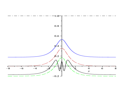
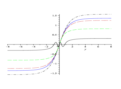
Figure 8: Symmetric solutions normalized, Eq. (49), for $\tilde{c}=1$; $m=0$ (dash-dotted black line), $m=1$ (solid blue line), $m=1.25$ (long-dashed red line), $m=2$ (dashed green line), and $m=10$ (solid black line).

Figure 9: Asymmetric solutions, Eq. (50), for $\tilde{c}=1$; $m=0$ (dash-dotted black line), $m=1$ (solid blue line), $m=2$ (long-dashed red line), $m=5$ (dashed green line), and $m=10$ (black line).

In the region of interest, $z<1$, regular local solutions around $z=0$ are defined by the Heun series

$$Hc(z)=\sum_{n=0}^{\infty}d_{n}\,z^{n},$$ (44)

where the constants $d_{n}$ (with $d_{-1}=0$ and $d_{0}=1$) are determined by the three-term recurrence relation FIZIEV

$$A_{n}d_{n}=B_{n}d_{n-1}+C_{n}d_{n-2}$$ (45)

with

$$A_{n} = 1+\frac{\beta}{n}\rightarrow 1-\frac{1}{2n}$$ (46)

$$B_{n} = 1+\frac{-\alpha+\beta+\gamma-1}{n}$$ (47)

$$+ \frac{\eta+(\alpha-\beta-\gamma)/2-\alpha\beta/2+\beta\gamma/2}{n^{2}}$$

$$\rightarrow 1+\frac{m-\tilde{c}/2-3/2}{n}$$

$$+ \frac{\tilde{c}/2+1/2-m^{2}/4+3m/4}{n^{2}}$$

$$C_{n} = \frac{1}{n^{2}}\left(\delta+\frac{\alpha(\beta+\gamma)}{2}+\alpha(n-1)\right)$$ (48)

$$\rightarrow \frac{m^{2}}{4n^{2}}+\frac{m}{n^{2}}\left(n-\tilde{c}-\frac{5}{4}\right).$$

We can identify $\alpha=m$, $\beta=-1/2$, $\gamma=-\tilde{c}/2$, $\delta=m^{2}/4$, and $\eta=\tilde{c}/8+1/4-m^{2}/4$ by comparing Eqs. (40) and (41). The solutions to Eq. (18) are therefore given by

$$w^{(1)}(y)=e^{\frac{m}{2}\tanh^{2}\!y}\times\leavevmode\nobreak\ \leavevmode\nobreak\ \leavevmode\nobreak\ \leavevmode\nobreak\ \leavevmode\nobreak\ \leavevmode\nobreak\ \leavevmode\nobreak\ \leavevmode\nobreak\ \leavevmode\nobreak\ \leavevmode\nobreak\ \leavevmode\nobreak\ \leavevmode\nobreak\ \leavevmode\nobreak\ \leavevmode\nobreak\ \leavevmode\nobreak\ \leavevmode\nobreak\ \leavevmode\nobreak\ \leavevmode\nobreak\ \leavevmode\nobreak\ \leavevmode\nobreak\ \leavevmode\nobreak\ \leavevmode\nobreak\ \leavevmode\nobreak\ \leavevmode\nobreak\ \leavevmode\nobreak\ \leavevmode\nobreak\ \leavevmode\nobreak\ \leavevmode\nobreak\ \leavevmode\nobreak\ \leavevmode\nobreak\ \leavevmode\nobreak\ \leavevmode\nobreak\ \leavevmode\nobreak\ \leavevmode\nobreak\ \leavevmode\nobreak\ \leavevmode\nobreak\ \leavevmode\nobreak\ \leavevmode\nobreak\ \leavevmode\nobreak\ \leavevmode\nobreak\ \leavevmode\nobreak\ \leavevmode\nobreak\ \leavevmode\nobreak\ \leavevmode\nobreak\ \leavevmode\nobreak\ \leavevmode\nobreak\ \leavevmode\nobreak\$$

$$Hc\left(m,-\frac{1}{2},-\frac{\tilde{c}}{2},\frac{m^{2}}{4},\frac{1}{4}+\frac{\tilde{c}}{8}-\frac{m^{2}}{4};\,\tanh^{2}\!y\right)\leavevmode\nobreak\ \leavevmode\nobreak\ \leavevmode\nobreak\ \leavevmode\nobreak\ \leavevmode\nobreak\ \leavevmode\nobreak\$$ (49)

$$w^{(2)}(y)=e^{\frac{m}{2}\tanh^{2}\!y}\tanh\!y\times\leavevmode\nobreak\ \leavevmode\nobreak\ \leavevmode\nobreak\ \leavevmode\nobreak\ \leavevmode\nobreak\ \leavevmode\nobreak\ \leavevmode\nobreak\ \leavevmode\nobreak\ \leavevmode\nobreak\ \leavevmode\nobreak\ \leavevmode\nobreak\ \leavevmode\nobreak\ \leavevmode\nobreak\ \leavevmode\nobreak\ \leavevmode\nobreak\ \leavevmode\nobreak\ \leavevmode\nobreak\ \leavevmode\nobreak\ \leavevmode\nobreak\ \leavevmode\nobreak\ \leavevmode\nobreak\ \leavevmode\nobreak\ \leavevmode\nobreak\ \leavevmode\nobreak\ \leavevmode\nobreak\ \leavevmode\nobreak\ \leavevmode\nobreak\ \leavevmode\nobreak\ \leavevmode\nobreak\ \leavevmode\nobreak\ \leavevmode\nobreak\ \leavevmode\nobreak\ \leavevmode\nobreak\ \leavevmode\nobreak\ \leavevmode\nobreak\ \leavevmode\nobreak\ \leavevmode\nobreak\ \leavevmode\nobreak\$$

$$Hc\left(m,\frac{1}{2},-\frac{\tilde{c}}{2},\frac{m^{2}}{4},\frac{1}{4}+\frac{\tilde{c}}{8}-\frac{m^{2}}{4};\,\tanh^{2}\!y\right)\leavevmode\nobreak\ \leavevmode\nobreak\ \leavevmode\nobreak\ \leavevmode\nobreak\ \leavevmode\nobreak\ \leavevmode\nobreak\ \leavevmode\nobreak\ \leavevmode\nobreak\$$ (50)

for arbitrary values of $\tilde{c}$, i.e. for any value of the dilaton coupling constant.

The criterium to select the relevant solutions, i.e. continuity and finiteness in the whole $y$ space, indicates that for positive $\tilde{c}$ the mass spectra are in fact continua and not just discrete as obtained in the previous section. In the quantum mechanics analog approach, the boundary conditions resulted too restrictive to allow for the whole spectrum of the original problem and quantization arose as a byproduct. However, it does not mean that the actual spectrum belongs to the continuum for every value of $\tilde{c}$. After a numerical survey, we observe that for all $\tilde{c}\leq 0$ the mass spectra are discrete even in the full approach (see e.g. Table 1 where we show all the first values of $m$ for $\tilde{c}=-1$; see also Fig. 11 and 11). For positive values, i.e. $\tilde{c}\in(0,6)$, on the other hand, arbitrary values of the mass allow nondivergent $w(y)$ solutions. To illustrate this point, in Fig. 9 and 9 we have chosen a generic value of $\tilde{c}$ to display the solutions for several arbitrary values of $m$. For the special cases of $\tilde{c}$ studied in the previous Section the results coincide, as expected. However, with the important difference that on top of the previously found sequence the mass spectra now obtained fulfill it to the continuum, including zero.

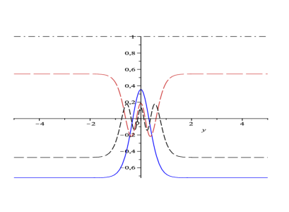
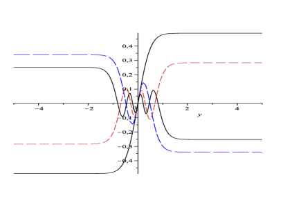
Figure 10: Symmetric solutions, Eq. (49), for $\tilde{c}=-1$ ($\gamma=2$); $m=0$ (dash-dotted black line), $m=5.01256460$ (solid blue line), $m=9.11222614$ (long-dashed red line), and $m=13.15839916$ (dashed black line).

Figure 11: Asymmetric solutions, Eq. (50), for $\tilde{c}=-1$ ($\gamma=2$); $m=2.88880921142$ (dash-dotted black line), $m=7.074052696$ (solid blue line), $m=11.138717717$ (long-dashed red line), and $m=15.173713228$ (solid black line). There is no massless mode in this set.

Table 1: List of the first values of $m_{s}$ (symmetric solutions) and $m_{a}$ (antisymmetric ones) for $\tilde{c}=-1$ ($\gamma=2$).

	$m_{s}$	$m_{a}$
	0.0000000	$--$
	5.01256460	2.88880921
	9.11222614	7.07405270
	13.15839916	11.13871772
	17.18603686	15.17371323
	21.20478031	19.19621044
	25.21848382	23.21211936
	29.22902086	27.22407315
	33.23742273	31.23344577
	37.24430826	35.24102973
	41.25007349	39.24731247

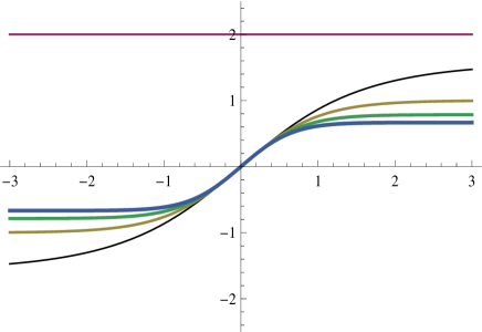
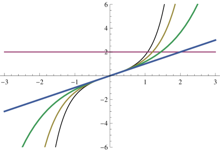
Figure 12: Some zero modes for $\tilde{c}>0$ (thinner to thicker): $w_{0}^{\tilde{c}=1}(y)=\arcsin(\tanh\!y)$; $w_{0}^{\tilde{c}=2}(y)=\tanh y$; $w_{0}^{\tilde{c}=3}(y)=\frac{1}{2}\left[\operatorname{sech}\!y\tanh\!y+\arcsin(\tanh\!y)\right]$; $w_{0}^{\tilde{c}=4}(x)=\frac{1}{3}\tanh\!y(3-\tanh^{2}\!y)$. A constant zero mode is present for any $\tilde{c}$.

Figure 13: Some zero-modes for $\tilde{c}\leq 0$ (thinner to thicker): $w_{0}^{\tilde{c}=-3}(y)=\frac{1}{3}\sinh\!y(3+\sinh^{2}\!y)$; $w_{0}^{\tilde{c}=-2}(y)=\frac{1}{2}(y+\sinh\!y\cosh\!y)$; $w_{0}^{\tilde{c}=-1}(y)=\sinh\!y$; $w_{0}^{\tilde{c}=0}(y)=y$. A constant zero-mode is present for any $\tilde{c}$.

4.1 The zero-mode of the Kalb-Ramond field

As a consequence of the previous analysis, we conclude that the quantum analog Schrodinger -like problem returns just a discrete cut of the spectrum and is therefore not fully appropriate to exhaustively solve the problem. In some cases, the zero-mode is not even manifest since eq. 20, with the appropriate boundary conditions at $z=\pm 1$, does not allow such a solution (see Sect. 3.1.2 and 3.1.1). A direct approach, on the other hand, allows an analytical $m=0$ solution to Eq. (17) for any value of $\tilde{c}$ :

$$w_{0}(y)=e_{1}+e_{2}\int^{y}\operatorname{sech}^{\tilde{c}}\!y\,dy.$$ (51)

After solving this integral the general zero-mode reads

$$w_{0}(y)=e_{1}+e_{2}\tanh\!y\ _{2}F_{1}\left(\frac{1}{2},\,\frac{1-\tilde{c}}{2},\,\frac{3}{2}\,;\,\tanh^{2}\!y\right)$$ (52)

which is finite everywhere provided $\tilde{c}$ is positive (see Figs. 13 and 13). Gauss hypergeometric functions are defined as ${}_{2}F_{1}\left(a,b,c;x\right)=1+\frac{a\ b\ x}{c\ 1!}+\frac{a(a+1)\ b(b+1)x^{2}}{c(c+1)\ 2!}+\dots\ .$ The constant solution $w_{0}(y)=e_{1}$ represents the symmetric zero-mode (it is of course finite and continuous for arbitrary $\tilde{c})$.

Thus, for $\tilde{c}>0$ there are two independent zero-modes while for $\tilde{c}\leq 0$ only the constant one. This was the result expected in the Schrodinger approach, where the ground-state must be symmetric. However, the associated boundary conditions precluded the zero-mode and the allowed ground state emerged as a massive mode (see e.g. Figs. 5 and 5). Independently of the approach, the gain of mass of the ground state may suggest unobservable the experimental signature of this field or, in turn, give important information about the dilatonic coupling indicating the exact value of the parameters of the model as we discuss in what follows.

5 Final discussion

Although the completeness of the Schrodinger approach is restricted to a particular range of parameters, it is plenty useful to evaluate the low energy features of the system, especially for negative values of $\tilde{c}$.

At very low energies we can compute the corresponding nonrelativistic effective potential to estimate the Kaluza-Klein contributions to the effective coupling to matter. Since the nonrelativistic potential, as given by the Green function of the equation of motion integrated along the source, depends on the square of the massive amplitudes at the origin, we must simply compare their relative weights to assess their contributions, see jaume .

We can assume that the coupling with the brane takes place exactly on the 4D ordinary space-time, at $y=0$. Since matter fields are constrained to the wall, it is precisely there that the relevant physical effects should be more important. As shown in Table 2, the normalized square amplitudes of the KK modes are rapidly decreasing with mass. In addition, each contribution to the effective nonrelativistic 4D static potential presents an exponential factor of the Yukawa type which also depends on the mass of the mode, further quenching the higher mass eigenstates (see also RS ; csakial for a study of this issue in the case of the gravitational field).

Table 2: List of first mass eigenstate square amplitudes at the origin; $\tilde{c}=-1$.

	$m_{s}$	$w_{m}^{2}(0)$
	0	1.00000000000
	5.01256460	0.35558755410
	9.11222614	0.19248779813
	13.15839916	0.13482515859
	17.18603686	0.10488449142
	21.20478031	0.08640457375
	25.21848382	0.07379433274
	29.22902086	0.06461526991
	33.23742273	0.05761117479
	37.24430826	0.05208093848
	41.25007349	0.04759600275

Thus, although KK excitations have nonvanishing momenta in the fifth direction interactions mediated by massive modes will be strongly suppressed near the braneworld.

Since the axion mass is expected to be very light but nonzero ($10^{-6}<m_{\chi}[\rm eV]<0.01$) nature06 , this particle would be just faintly coupled to matter fields and therefore hardly detectable by direct means matter axion . Although the experimental issues, several important collaborations are currently searching for an axion signal exp search axion .

In the present scenario, assuming that the axion is indeed a physical realization of the KR field, the eventual advent of an experimental result for the axion mass would suggest a value for the $\tilde{c}$ parameter in our model. A way to see this could be in principle accomplished by means of a detailed (and lengthy) inspection of a sufficiently large number of spectra for different values of $\tilde{c}$ until one finds the eigenvalue that better fits the experimental mass. For this, it would be necessary to fix the $b$ parameter in first place. If the axion happened to be massless we could associate a positive $\tilde{c}$. In this case, however, this prediction would be not very useful since we would not know exactly which particular value of $\tilde{c}$ between 0 and 6 (remember that for every positive $\tilde{c}$ there is a zero mode and no gap). As a matter of fact, this possibility is unlikely in face of the current experimental expectancy of a light but nonzero mass axion. Indeed, assuming that a mass gap exists in the physical spectrum of this particle, our model would associate a negative $\tilde{c}$ to the experimental mass, as explained above. For each value of $\tilde{c}$ we can compare its minimum eigenvalue to the axion mass. If we first transform $y\rightarrow\kappa y$ in eq.18, which results in a scaling of the mass $m_{n}^{2}\rightarrow m_{n}^{2}/\kappa^{2}\equiv m_{\chi}^{2}$, we will get a range of values of $\kappa$ for a range in $m_{\chi}$. For instance, let us choose $\tilde{c}=-1$ so that $m_{1}=5.01256460$. For an axion mass in $10^{-6}<m_{\chi}[\rm eV]<10^{-2}$ then $9.9174\times 10\approx 100>\kappa^{-1}[\rm cm]>9.9174\times 10^{-5}\approx 0.0001$, characterizing the size of the scale transformation. Now, since this parameter is defined as $\tilde{c}=-3(15+4\lambda\sqrt{3M^{3}})$ one could thereon get a theoretical prediction of the product $\lambda M^{3/2}$. Recall that the 5D Planck mass $M$ depends $M_{P}$ and $b$ through eq.11.

The study of the interaction of this field with the photon axion-photon by means of a mixed Maxwell-Kalb-Ramond lagrangian would allow for an additional theoretical tool to bear the axion problem. If it is true that the Kalb-Ramond axion supplies the spacetime with torsion in its nearness, a kind of primordial optical activity would be possible. Indeed, a non-Faraday rotation, independent of the wavelength and parameters of the source and intergalactic medium, has already been predicted in indianos EPJ 2002 . An optical rotation of the plane of polarization of light coming from distant sources rotation might then be observed in some near future. A signal of this effect would provide evidence of the existence of a primordial KR field and hence of a likely component of cold dark matter in the universe. This is being subject of further investigation.

References

- (1) L. Randall and R. Sundrum, Phys. Rev. Lett. 83, 4690 (1999); Phys. Rev. Lett. 83 (1999) 3370.
- (2) J.Polchinski, String Theory, vols. 1 & 2, (Cambridge University Press, Cambridge, England, 1998).
- (3) A. Kehagias and K. Tamvakis, Phys. Lett. B 504, 38 (2001).
- (4) M. S. Cunha, H. R. Christiansen, Phys. Rev. D 84, 085002 (2011).
- (5) Yu-Xiao Liu, Heng Guo, Chun-E Fu, Hai-Tao Li, Phys.Rev. D84 (2011) 044033. J. E. Thompson, R. R. Volkas, Phys.Rev. D82 (2010) 116007. Hai-Tao Li, Yu-Xiao Liu, Zhen-Hua Zhao, Heng Guo, Phys.Rev. D83 (2011) 045006.
- (6) Ashoke Sen, An Introduction to nonperturbative string theory, in A Newton Institute Euroconference On Duality And Supersymmetric Theories, 7-18 Apr 1997, Cambridge, England. Edited by D.I. Olive, P.C. West. Cambridge, Cambridge Univ. Press, 1999.
- (7) M. Kalb, P. Ramond Phys. Rev. D 9 (1974) 2273.
- (8) S.J. Gates, M. Grisaru, M. Rocek, W. Siegel, Superspace, W.A. Benjamin, New York 1983.
- (9) M. Green, J. Schwarz, E. Witten, Superstring theory, vol. II, Cambridge 1985.
- (10) H. R. Christiansen, M. S. Cunha, M. K. Tahim, Phys. Rev. D 82, 085023 (2010).
- (11) A.E. Chumbes, J.M. Hoff da Silva, M.B. Hott, arXiv:1108.3821; Yu-Xiao Liu, Chun-E Fu, Heng Guo, Hai-Tao Li, arXiv:1102.4500; W.T. Cruz, M.O. Tahim, C.A. Almeida, Europhys. Lett. 88 (2009) 41001; A.R. Lugo, M. B. Sturla, Phys.Lett. B637 (2006) 338.
- (12) P. Majumdar, S. SenGupta, Class. Quantum Grav. 16 (1999) L89 L94.
- (13) R. Puntigam, E. Schrufer, F. Hehl, Class. Quantum Grav. 14 (1997) 1347.
- (14) F. Hehl, P. von der Heyde, G. Kerlick, J. Nester, Rev. Mod. Phys. 48 (1976) 393.
- (15) S. SenGupta, A. Sinha, Phys. Lett. B 514 (2001) 109.
- (16) A. Lue, L. Wang, M. Kamionkowski, Phys. Rev. Lett. 83, (1999) 1506.
- (17) S. Kar, P. Majumdar, S. SenGupta, A. Sinha, Eur. Phys. J. C 23, 357 361 (2002).
- (18) M. Bowick, S. Giddings, J.A. Harvey, G.T. Horowitz, A. Strominger, Phys. Rev. Lett 61 (1988) 2823.
- (19) E. J. Copeland, R. Easther and D. Wands, Phys. Rev. D 56 (1997) 874.
- (20) D. Youm, Nucl. Phys. B 589, 315 (2000); idem, Phys. Rev. D64, 127501 (2001).
- (21) M. Cvetic, S. Griffies, S. Rey, Nucl. Phys. B 381, 301 (1992).
- (22) Saurya Das, Anindya Dey, Soumitra SenGupta, Class. Quant. Grav. 23, L67 (2006);
- (23) Heun, K. Zur Theorie der Riemann’schen Functionen Zweiter Ordnung mit vier Verzweigungspunkten. Mathematische Annalen 33, 161-179 (1889). Avalable at http://www.digizeitschriften.de/main/dms/img/navi
- (24) A. Ronveaux (Editor), Heun’s differential equations (Oxford University Press, 1995).
- (25) M. N. Hounkonnou, A. Ronveaux, Appl. Math. Comp. 209, 421 (2009).
- (26) E. S. Cleb-Terrab, J. Phys: Math Gen. 37, 9923 (2004).
- (27) P. P Fiziev, J. Phys. A: Math. Theor. 43, 035203 (2010).
- (28) M. Abramowitz and I. A. Stegun, Handbook of Mathematical Functions with Formulas, Graphs, and Mathematical tables, National Bureau of Standards, Applied Mathematics Series 55 (U.S. GPO, Washington, DC, 1972).
- (29) J. Garriga, T. Tanaka, Phys. Rev. Lett. 84, 2778 (2000).
- (30) S. Lamoreaux, Nature Vol 441/4, 31, May 2006.
- (31) A.V. Derbin, et al. Phys. Rev. D83 (2011) 023505.
- (32) ADMX - Axion Dark Matter experiment, http://www.phys.washington.edu/groups/admx/home.html; CAST - CERN Axion Solar Telescope, http://cast.web.cern.ch/CAST/index.html; CARRACK - Cosmic Axion Research using Rydberg Atoms in a resonant Cavity in Kyoto; PVLAS - Polarizzazione del Vuoto con Laser, http://w3.ts.infn.it/experiments/pvlas/
- (33) K. Zioutas et al., Phys. Rev. Lett. 94, 121301 (2005); E. Masso and J. Redondo, J. Cosmol. Astropart. Phys. 09 (2005) 015. O. Mena, S. Razzaque, F. Villaescusa Navarro. JCAP 1102 (2011) 030.
- (34) B. Nodland, J. Ralston Phys. Rev. Lett. 78 (1997) 3043.