Correlations in the Bose & Fermi Hubbard Model

Abstract

We study the Bose-Hubbard and Fermi-Hubbard model in the limit of large coordination numbers $Z$ (i.e., many tunnelling partners). Via a controlled expansion into powers of $1/Z$, we establish a hierarchy of correlations, which facilitates an approximate analytic solution of the quantum evolution. For the Bose-Hubbard model, we derive the growth of phase coherence after a quench from the Mott to the superfluid phase. For a quench within the Mott phase, we find that various local observables approach a quasi-equilibrium state after a finite period of time. However, this state is not thermal, i.e., real thermalisation – if it occurs – requires much longer time scales. For a tilted lattice in the Mott state, we calculate the tunnelling probability and find a remarkable analogy to the Sauter-Schwinger effect (i.e., electron-positron pair creation out of the vacuum due to a strong electric field). These analytical results are compared to numerical simulations for finite lattices in one and two dimensions and we find qualitative agreement. Finally, we generalise these studies to the more involved case of the Fermi-Hubbard model.

1 Introduction

The theoretical description of strongly interacting many-particle quantum systems in condensed matter physics is a difficult undertaking in general. Even in those cases where it is possible to derive a Hamiltonian which contains all relevant parts for a complete description of the many-particle system under consideration, a complete solution of the dynamics or an exact evaluation of the ground state is often out of reach.

However, essential features such as phase transitions or quasi-particle excitations are already contained in drastically simplified models. One of the most studied models which describes strongly interacting electrons in a solid is the Fermi-Hubbard model [1, 2, 3]. Although it describes only the physics of a single energy band without long-ranged Coulomb-interactions, it is believed to exhibit various interesting phenomena such as the metal-insulator transition, anti-ferromagnetism, ferrimagnetism, ferromagnetism, Tomonaga-Luttinger liquid, and superconductivity [4]. The Fermi-Hubbard model was first established by J. Hubbard in order to describe correlations of electrons in narrow energy bands [1, 2, 3]. It connects the Heitler-London theory of strongly interacting electrons on one side and the band theory, valid for weak interactions, on the other side.

Apart from electrons in solids, there are also other physical systems which can be described (within suitable approximations) by the Fermi-Hubbard model, for example ultra-cold atoms in optical lattices. Since optical lattice systems allow for a tuning of the model parameters over a wide range (in contrast to most condensed matter systems), they are predestinated for the study of the fermionic Hubbard model. This has been experimentally realised by trapping fermionic Potassium atoms in an optical lattice [5, 6, 7]. By increasing the on-site interaction among the atoms, the transition from a metallic phase to a Mott insulating phase was deduced from compressibility measurements and in situ imaging [7].

After replacing the fermionic by bosonic atoms, the optical lattice system corresponds to the Bose-Hubbard model, which describes interacting bosons in periodic potentials. The Bose-Hubbard model was first motivated by experimental realisations such as Helium-4 absorbed in porous media or Cooper pairs in granular media [8]. Within the last decade, the Bose-Hubbard model has been attracting increasing attention due to its experimental realisation with interacting bosons, for example Rubidium atoms, in optical lattices [9, 10]. The phase diagram, which is much better understood than in the fermionic case, contains (for vanishing disorder) a superfluid regime and Mott insulating phases. The transition between the two phases is characterised by a natural order parameter, such as the superfluid density. This second-order quantum phase transition, which results from the competition between kinetic energy and on-site interaction, has been observed for bosons in optical lattices [9].

Though at first glance seemingly very simple, the fermionic as well as the bosonic lattice models are not exactly solvable in general, the only exceptions being the Fermi-Hubbard model in one dimension [11, 12] and trivial situations, such as the case of vanishing or infinitely strong interaction, or an empty lattice, for example. Thus, various analytical and numerical techniques have been developed to study their physical properties. Widely used numerical methods, ignoring distance-dependent quantum correlations between different lattice sites, are mean-field approaches such as the dynamical mean-field theory (DMFT) [13, 14]. Exact diagonalisation (analytical or numerical) is only possible for small system sizes [15, 16]. Monte Carlo methods can improve the situation [17], but they can sample only a small part of the whole Hilbert space and have problems with general time-dependent situations.

An important and widely used analytical approach is the Gutzwiller ansatz [18] – for the bosonic and the fermionic case. However, a serious drawback of this Gutzwiller mean-field approach is again the neglect of distance-dependent quantum correlations between different lattice sites. This simplification leads sometimes to unphysical behaviour – for example, the Mott-insulator state would not react to an external force within the Gutzwiller mean-field approach.

The main goal of the present work is to study these non-local quantum correlations in the Bose and Fermi-Hubbard models. To this end, we develop an analytical expansion in powers of the inverse coordination number $Z$ (i.e., the number of tunnelling partners of a given lattice site). For comparison, we also calculated these non-local quantum correlations by means of exact (numerical) diagonalisation for one and two-dimensional lattices. Although exact diagonalisation is possible only for small systems, the results are in good agreement with those obtained by the analytical expansion and the Density Matrix Renormalisation Group technique (DMRG) [19, 20].

The paper is organised as follows. After a brief introduction into the Bose-Hubbard model in Sec. 2, we present our analytical method for general Hubbard type Hamiltonians in Section 3. With this method, the ground state properties of the bosonic Mott insulator phase are derived in Sec. 4. Taking this Mott insulator as the initial state, the temporal evolution of the correlations after a quantum quench to the superfluid regime as well as within the Mott phase are studied in Sections 5 and 6. In Section 7, we investigate particle-hole pair creation out of the (bosonic) Mott state induced by a weak tilt of the lattice and establish a quantitative analogy to electron-positron pair creation due to a strong electric field (Sauter-Schwinger effect) in Sec. 8. The results of Secs. 4–8 are derived in first order $1/Z$ (where $Z$ is the coordination number). In Section 9, we show how to extend our analytical method to higher orders in $1/Z$. Subsequently, we compare our analytical results with exact numerical studies of finite bosonic lattices in Section 10 and find qualitative agreement.

In the second part of the paper, we consider similar problems for fermions. After a brief introduction into the Fermi-Hubbard model in Section 11, we discuss its ground state correlations (in the fermionic Mott state) and quench dynamics Secs. 12 and 13. Section 14 is then devoted to particle-hole pair creation induced by a weak lattice tilt. Finally, we address resonant tunnelling in the Bose and Fermi-Hubbard model due to a large lattice tilt in Section 15.

2 Bose-Hubbard Model

The Bose-Hubbard model is one of the most simple and yet non-trivial models in condensed matter theory [8, 21, 22]. It describes identical bosons hopping on a lattice with the tunnelling rate $J$. In addition, two (or more) bosons at the same lattice site repel each other with the interaction energy $U$. The Hamiltonian reads

$$\hat{H}=-\frac{J}{Z}\sum_{\mu\nu}T_{\mu\nu}\hat{b}^{\dagger}_{\mu}\hat{b}_{\nu}+\frac{U}{2}\sum_{\mu}\hat{n}_{\mu}(\hat{n}_{\mu}-1)\,.$$ (1)

Here $\hat{b}^{\dagger}_{\mu}$ and $\hat{b}_{\nu}$ are the creation and annihilation operators at the lattice sites $\mu$ and $\nu$, respectively, which obey the usual commutation relations

$$\left[\hat{b}_{\nu},\hat{b}_{\mu}^{\dagger}\right]=\delta_{\mu\nu}\;,\,\left[\hat{b}_{\nu}^{\dagger},\hat{b}_{\mu}^{\dagger}\right]=\left[\hat{b}_{\nu},\hat{b}_{\mu}\right]=0\,.$$ (2)

The lattice structure is encoded in the adjacency matrix $T_{\mu\nu}$ which equals unity if $\mu$ and $\nu$ are tunnelling neighbours (i.e., if a particle can hop from $\mu$ to $\nu$) and zero otherwise. The number of tunnelling neighbours at a given site $\mu$ yields the coordination number $Z=\sum_{\nu}T_{\mu\nu}$ (we assume a translationally invariant lattice). Finally, $\hat{n}_{\mu}=\hat{b}^{\dagger}_{\mu}\hat{b}_{\mu}$ is the number operator and we assume unit filling $\langle\hat{n}_{\mu}\rangle=1$ in the following. Note that the total particle number $\hat{N}=\sum_{\mu}\hat{n}_{\mu}$ is conserved $[\hat{H},\hat{N}]=0$.

The Bose-Hubbard model is considered [23] one of the prototypical examples for a quantum phase transition. If the interaction term dominates $U\gg J$, the bosons are pinned to their lattice sites and we have the Mott insulator state

$$\left|\Psi_{\rm Mott}\right>_{J=0}=\bigotimes\limits_{\mu}\left|1\right>_{\mu}=\prod\limits_{\mu}\hat{b}_{\mu}^{\dagger}\left|0\right>\;\leadsto\;\hat{H}\left|\Psi_{\rm Mott}\right>_{J=0}=0\,,$$ (3)

which is fully localised. If the hopping rate dominates $U\ll J$, on the other hand, the particles can propagate freely across the lattice and become completely delocalised

$$\left|\Psi_{\rm superfluid}\right>_{U=0}=\frac{1}{\sqrt{N!}}\left(\hat{b}_{\mbox{\boldmath$\scriptstyle k$}=0}^{\dagger}\right)^{N}\left|0\right>=\frac{1}{\sqrt{N!N^{N}}}\left(\sum_{\mu}\hat{b}_{\mu}^{\dagger}\right)^{N}\left|0\right>\,,$$ (4)

which is the superfluid phase. Obviously, the Mott state (3) does not have any correlations, for example $\langle\hat{b}^{\dagger}_{\mu}\hat{b}_{\nu}\rangle_{\rm Mott}=\delta_{\mu\nu}$, whereas the superfluid state in (4) shows correlations across the whole lattice $\langle\hat{b}^{\dagger}_{\mu}\hat{b}_{\nu}\rangle_{\rm superfluid}=1$. Furthermore, the Mott insulator state is separated by a finite energy gap from the lowest excited state, while the superfluid state possesses sound-like modes with arbitrarily low energies (for an infinitely large lattice $N\uparrow\infty$). Finally, the Bose-Hubbard model can be realised experimentally (to a very good approximation) with ultra-cold atoms in optical lattices [24, 25, 26] and it was even possible to observe the aforementioned phase transition in these systems [9].

In spite of its simplicity, the Bose-Hubbard model (1) cannot be solved analytically. Numerical simulations are limited to reduced sub-spaces or small systems sizes, see Section 10 below. Analytical approaches are based on suitable approximations. In order to control the error of these approximations, they should be based on an expansion in term of some large or small control parameter. For the Bose-Hubbard model (1), one could consider the limit of large $\langle\hat{n}_{\mu}\rangle\gg 1$ or small $\langle\hat{n}_{\mu}\rangle\ll 1$ filling [27, 28], for example, or the limit of weak coupling $U\ll J$ or strong coupling $U\gg J$ [29, 30, 31]. However, none of these limits is particularly well suited for studying the Mott–superfluid phase transition. To this end, we consider the limit $Z\gg 1$ in the following and employ an expansion into powers of $1/Z$ as small control parameter. Note that an expansion in powers of $1/Z$ was also used to derive bosonic dynamical mean-field equations (which were then solved numerically) in [32, 33, 34].

3 Hierarchy of Correlations

Let us consider general Hamiltonians of the form

$$\hat{H}=\frac{1}{Z}\sum_{\mu\nu}\hat{H}_{\mu\nu}+\sum_{\mu}\hat{H}_{\mu}\,,$$ (5)

which includes the Bose-Hubbard model (1) as a special case. The quantum evolution of the density operator $\hat{\rho}$ describing the state of the full lattice can be written as

$$i\partial_{t}\hat{\rho}=\left[\hat{H},\hat{\rho}\right] = \frac{1}{Z}\sum_{\mu\nu}\left[\hat{H}_{\mu\nu},\hat{\rho}\right]+\sum_{\mu}\left[\hat{H}_{\mu},\hat{\rho}\right]$$ (6)

$$= \frac{1}{Z}\sum_{\mu\nu}\,{\cal L}_{\mu\nu}\hat{\rho}+\sum_{\mu}\,{\cal L}_{\mu}\hat{\rho}\,,$$

where we have introduced the Liouville super-operators $\,{\cal L}_{\mu\nu}$ and $\,{\cal L}_{\mu}$ as short-hand notation. As the next step, we introduce the reduced density matrices for one or more lattice sites via averaging (tracing) over all other sites

$$\hat{\rho}_{\mu} = \tr_{\not\mu}\{\hat{\rho}\}$$

$$\hat{\rho}_{\mu\nu} = \tr_{\not\mu\not\nu}\{\hat{\rho}\}\,,$$ (7)

and so on. Note that $\tr\{\hat{\rho}\}=1$ implies $\tr_{\mu}\{\hat{\rho}_{\mu}\}=1$ and $\tr_{\mu\nu}\{\hat{\rho}_{\mu\nu}\}=1$ etc. Since we are interested in the (quantum) correlations, we separate the correlated and uncorrelated parts of the reduced density matrices via

$$\hat{\rho}_{\mu\nu} = \hat{\rho}_{\mu\nu}^{\rm corr}+\hat{\rho}_{\mu}\hat{\rho}_{\nu}$$

$$\hat{\rho}_{\mu\nu\lambda} = \hat{\rho}_{\mu\nu\lambda}^{\rm corr}+\hat{\rho}_{\mu\nu}^{\rm corr}\hat{\rho}_{\lambda}+\hat{\rho}_{\mu\lambda}^{\rm corr}\hat{\rho}_{\nu}+\hat{\rho}_{\nu\lambda}^{\rm corr}\hat{\rho}_{\mu}+\hat{\rho}_{\mu}\hat{\rho}_{\nu}\hat{\rho}_{\lambda}\,,$$ (8)

and analogously for more lattice sites. As a consequence, we obtain from (6) the evolution equation for the on-site density matrix

$$i\partial_{t}\hat{\rho}_{\mu}=\frac{1}{Z}\sum_{\kappa\neq\mu}\tr_{\kappa}\left\{\,{\cal L}^{S}_{\mu\kappa}(\hat{\rho}^{\rm corr}_{\mu\kappa}+\hat{\rho}_{\mu}\hat{\rho}_{\kappa})\right\}+\,{\cal L}_{\mu}\hat{\rho}_{\mu}\,,$$ (9)

where $\,{\cal L}_{\mu\nu}^{S}=\,{\cal L}_{\mu\nu}+\,{\cal L}_{\nu\mu}$ denotes the symmetrised form. Obviously, solving this equation exactly requires knowledge of the two-point correlation $\hat{\rho}^{\rm corr}_{\mu\kappa}$. The time-evolution of this quantity can also obtained from (6) and reads

$$i\partial_{t}\hat{\rho}^{\rm corr}_{\mu\nu} = \,{\cal L}_{\mu}\hat{\rho}^{\rm corr}_{\mu\nu}+\frac{1}{Z}\,{\cal L}_{\mu\nu}(\hat{\rho}^{\rm corr}_{\mu\nu}+\hat{\rho}_{\mu}\hat{\rho}_{\nu})-\frac{\hat{\rho}_{\mu}}{Z}\tr_{\mu}\left\{\,{\cal L}^{S}_{\mu\nu}(\hat{\rho}^{\rm corr}_{\mu\nu}+\hat{\rho}_{\mu}\hat{\rho}_{\nu})\right\}$$ (10)

$$+\frac{1}{Z}\sum_{\kappa\not=\mu,\nu}\tr_{\kappa}\left\{\,{\cal L}^{S}_{\mu\kappa}(\hat{\rho}^{\rm corr}_{\mu\nu\kappa}+\hat{\rho}^{\rm corr}_{\mu\nu}\hat{\rho}_{\kappa}+\hat{\rho}^{\rm corr}_{\nu\kappa}\hat{\rho}_{\mu})\right\}+(\mu\leftrightarrow\nu)\,.$$

As one would expect, this equation contains the three-point correlator $\hat{\rho}^{\rm corr}_{\mu\nu\kappa}$, and similarly the evolution equation for $\hat{\rho}^{\rm corr}_{\mu\nu\kappa\lambda}$ contains the four-point correlator etc. Consequently, one can never exactly solve this set of equations, truncated at any finite order.

However, the limit $Z\gg 1$ facilitates an approximate solution: Let us imagine that we start from an initial state $\hat{\rho}^{\rm in}=\bigotimes_{\mu}\hat{\rho}^{\rm in}_{\mu}$ without any correlations (i.e., $\hat{\rho}^{\rm corr}_{\mu\nu}=0$ and $\hat{\rho}^{\rm corr}_{\mu\nu\kappa}=0$, etc.) such as the Mott state (3). In this case, the right-hand side of (10) is suppressed by $\,{\cal O}(1/Z)$ and thus the time evolution creates only small correlations $i\partial_{t}\hat{\rho}^{\rm corr}_{\mu\nu}$. Moreover, if these correlations are small initially $\hat{\rho}^{\rm corr}_{\mu\nu}=\,{\cal O}(1/Z)$, they remain small – at least for a finite amount of time – because there is no term in (10) to compensate the $\,{\cal O}(1/Z)$ suppression. Note that the sum $\sum_{\kappa}$ in (10) might scale with $Z$, but this is compensated by the $1/Z$ factor in front of it. On the other hand, if we insert $\hat{\rho}^{\rm corr}_{\mu\nu}=\,{\cal O}(1/Z)$ into (9), we find that we can neglect this term and arrive at an approximate equation containing on-site density matrices only

$$i\partial_{t}\hat{\rho}_{\mu} = \frac{1}{Z}\sum_{\kappa\neq\mu}\tr_{\kappa}\left\{\,{\cal L}^{S}_{\mu\kappa}\hat{\rho}_{\mu}\hat{\rho}_{\kappa}\right\}+\,{\cal L}_{\mu}\hat{\rho}_{\mu}+\,{\cal O}(1/Z)$$ (11)

$$\approx \frac{1}{Z}\sum_{\kappa\neq\mu}\tr_{\kappa}\left\{\,{\cal L}^{S}_{\mu\kappa}\hat{\rho}_{\mu}\hat{\rho}_{\kappa}\right\}+\,{\cal L}_{\mu}\hat{\rho}_{\mu}\,,$$

The approximate solution $\hat{\rho}_{\mu}^{0}$ of this self-consistent equation is valid to lowest order in $1/Z$, i.e., $\hat{\rho}_{\mu}=\hat{\rho}_{\mu}^{0}+\,{\cal O}(1/Z)$ and reproduces the well-known Gutzwiller ansatz [18, 21, 35]. If we now insert this approximate solution $\hat{\rho}_{\mu}^{0}$ into (10), we get an approximate evolution equation for the two-point correlator

$$i\partial_{t}\hat{\rho}^{\rm corr}_{\mu\nu} = \,{\cal L}_{\mu}\hat{\rho}^{\rm corr}_{\mu\nu}+\frac{1}{Z}\,{\cal L}_{\mu\nu}\hat{\rho}^{0}_{\mu}\hat{\rho}^{0}_{\nu}+\frac{1}{Z}\sum_{\kappa\not=\mu,\nu}\tr_{\kappa}\left\{\,{\cal L}^{S}_{\mu\kappa}(\hat{\rho}^{\rm corr}_{\mu\nu}\hat{\rho}^{0}_{\kappa}+\hat{\rho}^{\rm corr}_{\nu\kappa}\hat{\rho}^{0}_{\mu})\right\}$$ (12)

$$-\frac{\hat{\rho}^{0}_{\mu}}{Z}\tr_{\mu}\left\{\,{\cal L}^{S}_{\mu\nu}\hat{\rho}^{0}_{\mu}\hat{\rho}^{0}_{\nu}\right\}+(\mu\leftrightarrow\nu)+\,{\cal O}(1/Z^{2})\,.$$

Note that we have assumed that the three-point correlations $\hat{\rho}^{\rm corr}_{\mu\nu\kappa}$ do not spoil this line of arguments and are suppressed by $\,{\cal O}(1/Z^{2})$ in complete analogy. This is indeed correct and can be shown in basically the same way, see Appendix 17. More generally, we find that $\ell$-point correlations are suppressed as $\,{\cal O}(1/Z^{\ell-1})$, i.e.,

$$\hat{\rho}_{\mu} = \,{\cal O}\left(Z^{0}\right)$$

$$\hat{\rho}^{\rm corr}_{\mu\nu} = \,{\cal O}\left(1/Z\right)$$

$$\hat{\rho}^{\rm corr}_{\mu\nu\kappa} = \,{\cal O}\left(1/Z^{2}\right)$$

$$\hat{\rho}^{\rm corr}_{\mu\nu\kappa\lambda} = \,{\cal O}\left(1/Z^{3}\right)\,,$$ (13)

and so on, see Appendix 17. This hierarchy (3) is related to the quantum de Finetti theorem [36], the generalised cumulant expansion [37], and the Bogoliubov-Born-Green-Kirkwood-Yvon (BBGKY) hierarchy [38], but we are considering lattice sites instead of particles. As an example for the four-point correlator, let us consider observables $\hat{A}_{\mu}$, $\hat{B}_{\nu}$, $\hat{C}_{\kappa}$, and $\hat{D}_{\lambda}$ at four different lattice sites, which have vanishing on-site expectation values $\langle\hat{A}_{\mu}\rangle=\langle\hat{B}_{\nu}\rangle=\langle\hat{C}_{\kappa}\rangle=\langle\hat{D}_{\lambda}\rangle=0$. In this case, the hierarchy (3) implies

$$\langle\hat{A}_{\mu}\hat{B}_{\nu}\hat{C}_{\kappa}\hat{D}_{\lambda}\rangle = \langle\hat{A}_{\mu}\hat{B}_{\nu}\rangle\langle\hat{C}_{\kappa}\hat{D}_{\lambda}\rangle+\langle\hat{A}_{\mu}\hat{C}_{\kappa}\rangle\langle\hat{B}_{\nu}\hat{D}_{\lambda}\rangle+\langle\hat{A}_{\mu}\hat{D}_{\lambda}\rangle\langle\hat{B}_{\nu}\hat{C}_{\kappa}\rangle$$ (14)

$$+\,{\cal O}\left(1/Z^{3}\right)\,,$$

which resembles the Wick theorem in free quantum field theory (even though the quantum system considered here is strongly interacting).

4 Mott Insulator State

Now let us apply the hierarchy discussed above to the Bose-Hubbard model (1). To this end, we start with the factorising Mott state (3) at zero hopping rate $J=0$ as our initial state

$$\hat{\rho}^{\rm in}=\bigotimes\limits_{\mu}\hat{\rho}^{\rm in}_{\mu}=\bigotimes\limits_{\mu}\left|1\right>_{\mu}\!\left<1\right|\,.$$ (15)

Then we slowly switch on the hopping rate $J(t)$ until we reach its final value. In view of the finite energy gap, the adiabatic theorem implies that we stay very close to the real ground state of the system if we do this slowly enough. Of course, we cannot cross the phase transition in this way (i.e., adiabatically) since the energy gap vanishes at the critical point, see Section 5 below.

Since we have $\langle\hat{b}_{\mu}\rangle=0$ in the Mott state, Eq. (11) simplifies to

$$i\partial_{t}\hat{\rho}_{\mu}\approx\frac{1}{Z}\sum_{\kappa\neq\mu}\tr_{\kappa}\left\{\,{\cal L}^{S}_{\mu\kappa}\hat{\rho}_{\mu}\hat{\rho}_{\kappa}\right\}+\,{\cal L}_{\mu}\hat{\rho}_{\mu}=0\,\leadsto\,\hat{\rho}_{\mu}^{0}=\left|1\right>_{\mu}\!\left<1\right|\,.$$ (16)

Thus, to zeroth order in $1/Z$ (i.e., on the Gutzwiller mean-field level), the Mott insulator state $\hat{\rho}_{\mu}^{0}$ for finite $J$ has the same form as for $J=0$. To obtain the first order in $1/Z$, we insert this result into (12). Again using $\langle\hat{b}_{\mu}\rangle=0$, we find

$$i\partial_{t}\hat{\rho}^{\rm corr}_{\mu\nu} = \left(\,{\cal L}_{\mu}+\,{\cal L}_{\nu}\right)\hat{\rho}^{\rm corr}_{\mu\nu}+\frac{1}{Z}\,{\cal L}_{\mu\nu}^{S}\hat{\rho}_{\mu}^{0}\hat{\rho}_{\nu}^{0}$$ (17)

$$+\frac{1}{Z}\sum_{\kappa\not=\mu,\nu}\tr_{\kappa}\left\{\,{\cal L}^{S}_{\mu\kappa}\hat{\rho}^{\rm corr}_{\nu\kappa}\hat{\rho}_{\mu}^{0}+\,{\cal L}^{S}_{\nu\kappa}\hat{\rho}^{\rm corr}_{\mu\kappa}\hat{\rho}_{\nu}^{0}\right\}+\,{\cal O}(1/Z^{2})\,.$$

Formally, this is an evolution equation for an infinite dimensional matrix $\hat{\rho}^{\rm corr}_{\mu\nu}$. Fortunately, however, it suffices to consider a few elements only. If we introduce $\hat{p}_{\mu}=\left|1\right>_{\mu}\!\left<2\right|$ and $\hat{h}_{\mu}=\left|0\right>_{\mu}\!\left<1\right|$ as local particle and hole operators, all the interesting physics can be captured by their correlation functions (for $\mu\neq\nu$)

$$f_{\mu\nu}^{11} = \langle\hat{h}^{\dagger}_{\mu}\hat{h}_{\nu}\rangle=\tr\left\{\hat{\rho}\,\hat{h}^{\dagger}_{\mu}\hat{h}_{\nu}\right\}=\tr_{\mu\nu}\left\{\hat{\rho}^{\rm corr}_{\mu\nu}\hat{h}^{\dagger}_{\mu}\hat{h}_{\nu}\right\}\,,$$

$$f_{\mu\nu}^{12} = \langle\hat{h}^{\dagger}_{\mu}\hat{p}_{\nu}\rangle=\tr\left\{\hat{\rho}\,\hat{h}^{\dagger}_{\mu}\hat{p}_{\nu}\right\}=\tr_{\mu\nu}\left\{\hat{\rho}^{\rm corr}_{\mu\nu}\hat{h}^{\dagger}_{\mu}\hat{p}_{\nu}\right\}\,,$$

$$f_{\mu\nu}^{21} = \langle\hat{p}^{\dagger}_{\mu}\hat{h}_{\nu}\rangle=\tr\left\{\hat{\rho}\,\hat{p}^{\dagger}_{\mu}\hat{h}_{\nu}\right\}=\tr_{\mu\nu}\left\{\hat{\rho}^{\rm corr}_{\mu\nu}\hat{p}^{\dagger}_{\mu}\hat{h}_{\nu}\right\}\,,$$

$$f_{\mu\nu}^{22} = \langle\hat{p}^{\dagger}_{\mu}\hat{p}_{\nu}\rangle=\tr\left\{\hat{\rho}\,\hat{p}^{\dagger}_{\mu}\hat{p}_{\nu}\right\}=\tr_{\mu\nu}\left\{\hat{\rho}^{\rm corr}_{\mu\nu}\hat{p}^{\dagger}_{\mu}\hat{p}_{\nu}\right\}\,.$$ (18)

To first order in $1/Z$, these correlation functions form a closed set of equations

$$i\partial_{t}f^{12}_{\mu\nu} = -\frac{J}{Z}\sum_{\kappa\neq\mu,\nu}\left(T_{\mu\kappa}(f^{12}_{\kappa\nu}+\sqrt{2}f^{22}_{\kappa\nu})+\sqrt{2}T_{\nu\kappa}(f^{11}_{\mu\kappa}+\sqrt{2}f_{\mu\kappa}^{12})\right)$$ (19)

$$+Uf^{12}_{\mu\nu}-\frac{J\sqrt{2}}{Z}T_{\mu\nu}$$

$$i\partial_{t}f^{21}_{\mu\nu} = +\frac{J}{Z}\sum_{\kappa\neq\mu,\nu}\left(T_{\nu\kappa}(f^{21}_{\kappa\mu}+\sqrt{2}f^{11}_{\kappa\mu})+\sqrt{2}T_{\mu\kappa}(f^{22}_{\kappa\nu}+\sqrt{2}f_{\kappa\nu}^{12})\right)$$ (20)

$$-Uf^{21}_{\mu\nu}+\frac{J\sqrt{2}}{Z}T_{\mu\nu}$$

$$i\partial_{t}f^{11}_{\mu\nu} = i\partial_{t}f^{22}_{\mu\nu}=-\frac{\sqrt{2}J}{Z}\sum_{\kappa\neq\mu,\nu}\left(T_{\mu\kappa}f_{\kappa\nu}^{21}-T_{\nu\kappa}f_{\mu\kappa}^{12}\right)\,.$$ (21)

This truncation is due to the fact that the correlation functions $f^{mn}_{\mu\nu}$ involving higher occupation numbers $m\geq 3$ or $n\geq 3$ do not have any source terms of order $1/Z$ and hence do not contribute at that level. Exploiting translational symmetry, we may simplify these equations by a spatial Fourier transformation with

$$T_{\mu\nu} = \frac{Z}{N}\sum_{\mathbf{k}}T_{\mathbf{k}}e^{i\mathbf{k}\cdot(\mathbf{x}_{\mu}-\mathbf{x}_{\nu})}$$ (22)

$$f^{ab}_{\mu\nu} = \frac{1}{N}\sum_{\mathbf{k}}f^{ab}_{\mathbf{k}}e^{i\mathbf{k}\cdot(\mathbf{x}_{\mu}-\mathbf{x}_{\nu})}\,,$$ (23)

where $N$ denotes the number of lattice sites (which equals the number of particles in our case). Formally, in order to Fourier transform equations (19-21), one should add the summands corresponding to $\kappa=\mu$ and $\kappa=\nu$. Since these terms are of order $1/Z^{2}$, they do not spoil our first-order analysis. However, when going to second order $1/Z^{2}$ (see Section 9 below), they have to be taken into account.

After the Fourier transformation (22) and (23), Eqs. (19-21) become

$$(i\partial_{t}-U+3JT_{\mathbf{k}})f_{\mathbf{k}}^{12} = -\sqrt{2}JT_{\mathbf{k}}(f_{\mathbf{k}}^{11}+f_{\mathbf{k}}^{22}+1)\,,$$ (24)

$$(i\partial_{t}+U-3JT_{\mathbf{k}})f_{\mathbf{k}}^{21} = +\sqrt{2}JT_{\mathbf{k}}(f_{\mathbf{k}}^{11}+f_{\mathbf{k}}^{22}+1)\,,$$ (25)

$$i\partial_{t}f_{\mathbf{k}}^{11}=i\partial_{t}f_{\mathbf{k}}^{22} = \sqrt{2}JT_{\mathbf{k}}(f^{12}_{\mathbf{k}}-f^{21}_{\mathbf{k}})\,.$$ (26)

From the last equation, we may infer an effective particle-hole symmetry $f_{\mathbf{k}}^{11}=f_{\mathbf{k}}^{22}$ valid to first order in $1/Z$. With this symmetry, any stationary state (such as the ground state) with $\partial_{t}f_{\mathbf{k}}^{ab}=0$ must obey the condition

$$f_{\mathbf{k}}^{12}=f_{\mathbf{k}}^{21}=\frac{\sqrt{2}JT_{\mathbf{k}}(2f_{\mathbf{k}}^{11}+1)}{U-3JT_{\mathbf{k}}}\,.$$ (27)

The remaining unknown quantity $f_{\mathbf{k}}^{11}$ can be obtained in the following way: The evolution equations (24-26) leave the following bilinear quantity invariant

$$\partial_{t}\left[f_{\mathbf{k}}^{11}(f_{\mathbf{k}}^{11}+1)-f_{\mathbf{k}}^{12}f_{\mathbf{k}}^{21}\right]=0\,,$$ (28)

which remains valid even for time-dependent $J(t)$. Thus, starting in the Mott state (3) at zero hopping rate $J=0$ with vanishing correlations $f_{\mathbf{k}}^{ab}(t=0)=0$, we get the additional condition $f_{\mathbf{k}}^{11}(f_{\mathbf{k}}^{11}+1)=f_{\mathbf{k}}^{12}f_{\mathbf{k}}^{21}$ for all times $t>0$. Thus, to first order in $1/Z$, the ground state correlations read (for $\mu\neq\nu$)

$$\langle\hat{h}^{\dagger}_{\mu}\hat{h}_{\nu}\rangle_{\rm ground}=\langle\hat{p}^{\dagger}_{\mu}\hat{p}_{\nu}\rangle_{\rm ground} = \frac{1}{N}\sum_{\mathbf{k}}\frac{U-3JT_{\mathbf{k}}-\omega_{\mathbf{k}}}{2\omega_{\mathbf{k}}}e^{i\mathbf{k}\cdot(\mathbf{x}_{\mu}-\mathbf{x}_{\nu})}$$ (29)

$$\langle\hat{h}^{\dagger}_{\mu}\hat{p}_{\nu}\rangle_{\rm ground}=\langle\hat{p}^{\dagger}_{\mu}\hat{h}_{\nu}\rangle_{\rm ground} = \frac{1}{N}\sum_{\mathbf{k}}\frac{\sqrt{2}JT_{\mathbf{k}}}{\omega_{\mathbf{k}}}e^{i\mathbf{k}\cdot(\mathbf{x}_{\mu}-\mathbf{x}_{\nu})}\,.$$ (30)

Here we have used the abbreviation [41]

$$\omega_{\mathbf{k}} = \sqrt{U^{2}-6JUT_{\mathbf{k}}+J^{2}T_{\mathbf{k}}^{2}}\,,$$ (31)

which is just the (non-zero) eigenfrequency of the evolution equations (24-26) for non-stationary states and will become important in the next Section.

The above equations (29) and (30) describe the correlations and are valid for $\mu\neq\nu$ only. The correct on-site density matrix $\rho_{\mu}$ can be obtained from (9) which shows that non-vanishing correlations lead to small deviations from the lowest-order result $\rho_{\mu}^{0}$. As one would expect, the quantum ground-state fluctuations manifest themselves in a small depletion of the unit-filling state $\hat{\rho}_{\mu}^{0}=\left|1\right>_{\mu}\!\left<1\right|$ given by a small but finite probability for a particle $f_{2}=\tr\{\hat{\rho}_{\mu}|2\rangle_{\mu}\langle 2|\}$ or a hole $f_{0}=\tr\{\hat{\rho}_{\mu}|0\rangle_{\mu}\langle 0|\}$. To first order in $1/Z$, we get from (9)

$$i\partial_{t}f_{0}=i\partial_{t}f_{2}=\sum_{\mathbf{k}}\frac{\sqrt{2}JT_{\mathbf{k}}}{N}(f_{\mathbf{k}}^{12}-f_{\mathbf{k}}^{21})=i\frac{1}{N}\sum_{\mathbf{k}}\partial_{t}f_{\mathbf{k}}^{11}\,,$$ (32)

where we used equation (26) in the last step. This equation can be integrated easily and with the initial conditions $f_{0}(t=0)=f_{2}(t=0)=0$ we find the $1/Z$-corrections to the one-site density matrix

$$\langle\hat{p}^{\dagger}_{\mu}\hat{p}_{\mu}\rangle=\langle\hat{h}_{\mu}\hat{h}^{\dagger}_{\mu}\rangle=f_{0}=f_{2}=\frac{1}{N}\sum_{\mathbf{k}}\frac{U-3JT_{\mathbf{k}}-\omega_{\mathbf{k}}}{2\omega_{\mathbf{k}}}\,.$$ (33)

Note that, even though the right-hand side of the above equation looks like that of (29) for $\mu=\nu$, one should be careful as they are derived from two different equations: (9) and (10).

5 Mott–Superfluid Quench

After having studied the ground state properties of the Mott phase, let us consider a quantum quench from the Mott state to the superfluid regime. This requires a time-dependent solution of the evolution equations (24-26) which crucially depends on the eigenfrequency (31). In view of the definition (22), $T_{\mathbf{k}}$ adopts its maximum value $T_{\mathbf{k}=0}=1$ at $\mathbf{k}=0$. Thus $\omega_{\mathbf{k}=0}=\Delta\mathcal{E}$ corresponds to the energy gap of the Mott state mentioned in Section 2. For $J=0$, we have a flat dispersion relation $\omega_{\mathbf{k}}=U$. If we increase $J$, the dispersion relation $\omega_{\mathbf{k}}$ bends down and the minimum at $\mathbf{k}=0$ approaches the axis. Finally, at a critical value of the hopping rate [42]

$$J_{\rm crit}=U(3-\sqrt{8})\,,$$ (34)

the minimum $\omega_{\mathbf{k}=0}$ touches the axis and thus the energy gap vanishes $\Delta\mathcal{E}=0$. This marks the transition to the superfluid regime and we cannot analytically or adiabatically continue beyond this point. However, nothing stops us from suddenly switching $J$ to a final value $J_{\rm out}>J_{\rm crit}$ beyond this point. Of course, this would not be adiabatic anymore and we would no longer be close to the ground state. For hopping rates $J$ which are a bit larger than the critical value $J>J_{\rm crit}$, the dispersion relation dives below the axis and the $\omega_{\mathbf{k}}^{2}$ become negative for small $\mathbf{k}$. Thus, the eigenfrequencies $\omega_{\mathbf{k}}$ become imaginary indicating an exponential growth of these modes, i.e., an instability. This is very natural since the quantum system “feels” that the Mott state is no longer the correct ground state.

If we consider even larger $J$, we find that the original minimum of the dispersion relation $\omega_{\mathbf{k}}^{2}$ at $\mathbf{k}=0$ splits into degenerate minima at finite values of $\mathbf{k}$ when $J=3U$, while $\mathbf{k}=0$ becomes a local maximum. This local maximum even emerges $\omega_{\mathbf{k}=0}^{2}>0$ on the positive side again for $J>U(3+\sqrt{8})$. Nevertheless, there are always unstable modes for some values of $\mathbf{k}$, see Fig. 1 and compare [43].

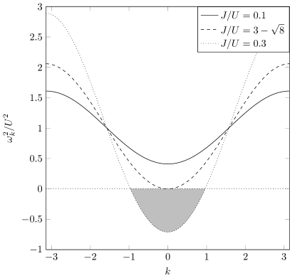
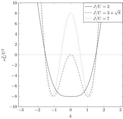
Figure 1: Dispersion relation $\omega_{k}^{2}/U^{2}$ in one dimension for different values of $J/U$.

After these preliminaries, let us study a quantum quench from the Mott state to the superfluid phase. For simplicity, we consider a sudden change of $J(t)=J\Theta(t)$ from $J=0$ to the final value of $J$ (but the calculation can easily be generalised to other scenarios). Solving the evolution equations (24-26) for this case, we find

$$\langle\hat{h}^{\dagger}_{\mu}\hat{h}_{\nu}\rangle_{\rm quench} = \langle\hat{p}^{\dagger}_{\mu}\hat{p}_{\nu}\rangle_{\rm quench}=\frac{1}{N}\sum_{\mathbf{k}}4J^{2}T_{\mathbf{k}}^{2}\,\frac{1-\cos(\omega_{\mathbf{k}}t)}{\omega^{2}_{\mathbf{k}}}\,e^{i\mathbf{k}\cdot(\mathbf{x}_{\mu}-\mathbf{x}_{\nu})}$$ (35)

$$\langle\hat{h}^{\dagger}_{\mu}\hat{p}_{\nu}\rangle_{\rm quench} = \frac{1}{N}\sum_{\mathbf{k}}\sqrt{2}JT_{\mathbf{k}}(U-3JT_{\mathbf{k}})\frac{1-\cos(\omega_{\mathbf{k}}t)}{\omega_{\mathbf{k}}^{2}}\,e^{i\mathbf{k}\cdot(\mathbf{x}_{\mu}-\mathbf{x}_{\nu})}$$ (36)

$$+\frac{i}{N}\sum_{\mathbf{k}}\sqrt{2}JT_{\mathbf{k}}\,\frac{\sin(\omega_{\mathbf{k}}t)}{\omega_{\mathbf{k}}}\,e^{i\mathbf{k}\cdot(\mathbf{x}_{\mu}-\mathbf{x}_{\nu})}\,.$$

The remaining correlation can simply be obtained via $\langle\hat{p}^{\dagger}_{\nu}\hat{h}_{\mu}\rangle=(\langle\hat{h}^{\dagger}_{\mu}\hat{p}_{\nu}\rangle)^{*}$. The correlator in terms of the original creation and annihilation operators $\hat{b}_{\mu}^{\dagger}$ and $\hat{b}_{\nu}$ is just a linear combination of these correlation functions

$$\langle\hat{b}_{\mu}^{\dagger}\hat{b}_{\nu}\rangle_{\rm quench}=\frac{1}{N}\sum_{\mathbf{k}}4JUT_{\mathbf{k}}\,\frac{1-\cos(\omega_{\mathbf{k}}t)}{\omega^{2}_{\mathbf{k}}}\,e^{i\mathbf{k}\cdot(\mathbf{x}_{\mu}-\mathbf{x}_{\nu})}\,.$$ (37)

Note that the momentum distribution

$$P(\mathbf{k})=\frac{1}{N^{2}}\sum_{\mathbf{\mu\nu}}e^{i\mathbf{k}\cdot(\mathbf{x}_{\mu}-\mathbf{x}_{\nu})}\langle\hat{b}_{\mu}^{\dagger}\hat{b}_{\nu}\rangle$$ (38)

which is basically the Fourier transform of $\langle\hat{b}_{\mu}^{\dagger}\hat{b}_{\nu}\rangle$, can be measured by time-of-flight experiments [9, 44] The quench $J(t)$ can be realised experimentally by decreasing the intensity of the laser field generating the optical lattice (which lowers the potential barrier for tunnelling and thus increases $J$). Thus the above prediction should be testable in experiments.

As explained above, after a quench to the superfluid regime, the frequencies $\omega_{\mathbf{k}}$ become imaginary for some $\mathbf{k}$ and thus these modes grow exponentially. As a result, the expectation value will quickly be dominated by these fast growing modes and so most of the details of the initial state will become unimportant. Of course, this exponential growth cannot continue forever – after some time, the $1/Z$-expansion breaks down since the quantum fluctuation are too strong and the growth will saturate.

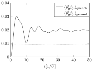
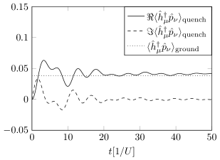
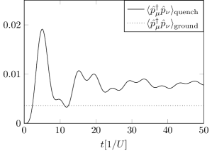
Figure 2: Time-dependence of the depletion $\langle\hat{p}_{\mu}^{\dagger}\hat{p}_{\mu}\rangle$ and the nearest-neighbor correlations functions $\langle\hat{h}_{\mu}^{\dagger}\hat{p}_{\nu}\rangle$ and $\langle\hat{p}_{\mu}^{\dagger}\hat{p}_{\nu}\rangle$ in three dimensions after the quench within the Mott phase from $J/U=0$ to $J/U=0.14$ in comparison to their ground state values. After quasi-equilibration, $\langle\hat{p}_{\mu}^{\dagger}\hat{p}_{\nu}\rangle_{\mathrm{quench}}$ and $\langle\hat{p}_{\mu}^{\dagger}\hat{p}_{\nu}\rangle_{\mathrm{ground}}$ as well as $\langle\hat{p}_{\mu}^{\dagger}\hat{p}_{\mu}\rangle_{\mathrm{quench}}$ and $\langle\hat{p}_{\mu}^{\dagger}\hat{p}_{\mu}\rangle_{\mathrm{ground}}$ differ roughly by a factor of two.

6 Equilibration versus Thermalisation

Instead of a quench from the Mott to the superfluid phase, we can also study a quench within the Mott regime. Again, we consider a sudden change of $J$ from zero its final value for simplicity – but now the final value $J$ lies below the critical point $J<J_{\rm crit}$. In this case, all frequencies are real $\omega_{\mathbf{k}}\in\mathbb{R}$ and thus there is no exponential growth – all modes oscillate. Apart from this point, we can use the same solution as in (35-37). For an infinite (or at least extremely large) lattice, the oscillations in (35-37) average out for sufficiently large times $t$ and thus these observables approach a quasi-equilibrium value

$$\langle\hat{h}^{\dagger}_{\mu}\hat{h}_{\nu}\rangle_{\rm equil}=\langle\hat{p}^{\dagger}_{\mu}\hat{p}_{\nu}\rangle_{\rm equil} = \frac{1}{N}\sum_{\mathbf{k}}\frac{4J^{2}T_{\mathbf{k}}^{2}}{\omega^{2}_{\mathbf{k}}}\,e^{i\mathbf{k}\cdot(\mathbf{x}_{\mu}-\mathbf{x}_{\nu})}$$ (39)

$$\langle\hat{h}^{\dagger}_{\mu}\hat{p}_{\nu}\rangle_{\rm equil}=\langle\hat{p}^{\dagger}_{\mu}\hat{h}_{\nu}\rangle_{\rm equil} = \frac{1}{N}\sum_{\mathbf{k}}\sqrt{2}JT_{\mathbf{k}}\,\frac{U-3JT_{\mathbf{k}}}{\omega_{\mathbf{k}}^{2}}e^{i\mathbf{k}\cdot(\mathbf{x}_{\mu}-\mathbf{x}_{\nu})}\,.$$ (40)

The quasi-equilibrium values for the local (on-site) particle or hole probability can be derived in complete analogy to the previous case

$$\langle\hat{p}^{\dagger}_{\mu}\hat{p}_{\mu}\rangle_{\rm equil}=\langle\hat{h}_{\mu}\hat{h}^{\dagger}_{\mu}\rangle_{\rm equil}=\frac{1}{N}\sum_{\mathbf{k}}\frac{4J^{2}T_{\mathbf{k}}^{2}}{\omega^{2}_{\mathbf{k}}}\,.$$ (41)

Having found that the observables considered above approach a quasi-equilibrium state, it is natural to ask the question of thermalisation. This is one of the major unsolved questions (or rather a set of questions) in quantum many-body theory [45, 46, 47, 48, 49] In one version, this question can be posed in the following way: Given an interacting quantum many-body system (for example the Bose-Hubbard model) on an infinite lattice in a appropriately excited state (such as after a quench), do all localised observables (e.g., $\langle\hat{p}^{\dagger}_{\mu}\hat{p}_{\mu}\rangle$ and $\langle\hat{h}^{\dagger}_{\mu}\hat{h}_{\nu}\rangle$) settle down to a value which is consistent with a thermal state described by a suitable temperature?

Even though we cannot settle this question here, we can compare the quasi-equilibrium values obtained above with a thermal state. To this end, we derive the thermal density matrix $\hat{\rho}_{\beta}$ corresponding to a given (inverse) temperature $k_{\rm B}T=1/\beta$. Using the grand canonical ensemble, the thermal density operator is given by

$$\hat{\rho}_{\beta}=\frac{e^{-\beta(\hat{H}-\mu\hat{N})}}{\tr\{e^{-\beta(\hat{H}-\mu\hat{N})}\}}\,,$$ (42)

where chemical potential $\mu$ will be chosen such that the filling is equal to unity. Since we cannot calculate $\hat{\rho}_{\beta}$ exactly, we employ strong-coupling perturbation theory, i.e., an expansion in powers of $J$. It is useful to introduce the operator [51]

$$\hat{R}(\beta)=e^{\beta\hat{H}_{0}}e^{-\beta(\hat{H}_{0}+\hat{H}_{1})}\,,$$ (43)

where $\hat{H}_{0}$ is the diagonal on-site part of the grand canonical Hamiltonian $\hat{H}-\mu\hat{N}$ and $\hat{H}_{1}$ is the hopping term. This operator satisfies the differential equation

$$\partial_{\beta}\hat{R}(\beta)=-\hat{H}_{1}(\beta)\hat{R}(\beta)\,,$$ (44)

where $\hat{H}_{1}(\beta)=e^{\beta\hat{H}_{0}}\hat{H}_{1}e^{-\beta\hat{H}_{0}}$. In analogy to time-dependent perturbation theory, the operator $\hat{R}$ can be calculated perturbatively by integrating this equation with respect to $\beta$. In first-order perturbation expansion, we have

$$\hat{\rho}_{\beta}=\frac{e^{-\beta\hat{H}_{0}}}{\tr\{e^{-\beta\hat{H}_{0}}\}}\left(1+\frac{J}{Z}\sum_{\mu\nu}T_{\mu\nu}\,\frac{e^{\beta U(\hat{n}_{\mu}-\hat{n}_{\nu}-1)}-1}{U(\hat{n}_{\mu}-\hat{n}_{\nu}-1)}\,\hat{a}^{\dagger}_{\mu}\hat{a}_{\nu}+\,{\cal O}(J^{2})\right)\,.$$ (45)

Obviously, the correction to first order in $J$ does not affect the on-site density matrix $\hat{\rho}_{\mu}$ but the two-point correlations. Thus, we find that the quasi-equilibrium state of the on-site density matrix $\hat{\rho}_{\mu}$ can indeed be described by a thermal state provided that we choose the chemical potential as $\mu=U/2$ which gives

$$\hat{\rho}_{\mu}(\beta)\approx\frac{e^{-\beta U/2}}{2}\,\left|0\right>_{\mu}\!\left<0\right|+\left(1-e^{-\beta U/2}\right)\left|1\right>_{\mu}\!\left<1\right|+\frac{e^{-\beta U/2}}{2}\,\left|2\right>_{\mu}\!\left<2\right|\,.$$ (46)

The particular value $\mu=U/2$ of the chemical potential ensures that (in first order thermal perturbation theory) we have on average one particle per lattice site and the particle-hole symmetry $\langle\hat{p}_{\mu}^{\dagger}\hat{p}_{\mu}\rangle=\langle\hat{h}_{\mu}^{\dagger}\hat{h}_{\mu}\rangle$. To obtain the correct probabilities, we have to select the temperature according to

$$e^{-\beta U/2}=2\langle\hat{p}^{\dagger}_{\mu}\hat{p}_{\mu}\rangle_{\rm equil}=\frac{2}{N}\sum_{\mathbf{k}}\frac{4J^{2}T_{\mathbf{k}}^{2}}{\omega^{2}_{\mathbf{k}}}=\,{\cal O}(1/Z)\,,$$ (47)

which can be deduced from (41) and (46). Since the depletion is small $\langle\hat{p}^{\dagger}_{\mu}\hat{p}_{\mu}\rangle=\,{\cal O}(1/Z)$, we obtain a low effective temperature which scales as $T=\,{\cal O}(U/\ln Z)$. Accordingly, consistent with our $1/Z$-expansion, we can neglect higher Boltzmann factors such as $e^{-\beta U}$.

Of course, the fact that the on-site density matrix $\hat{\rho}_{\mu}$ can be described (within our limits of accuracy) by a thermal state does not imply that the same is true for the correlations. To study this point, let us calculate the thermal two-point correlator from (45). To first order in $J$ and $1/Z=\,{\cal O}(e^{-\beta U}/2)$, we find

$$\langle\hat{h}^{\dagger}_{\mu}\hat{p}_{\nu}\rangle_{\beta}=\langle\hat{p}^{\dagger}_{\mu}\hat{h}_{\nu}\rangle_{\beta}=\frac{\sqrt{2}JT_{\mu\nu}}{ZU}+\,{\cal O}(J^{2})+\,{\cal O}(1/Z^{2})\,,$$ (48)

while $\langle\hat{h}^{\dagger}_{\mu}\hat{h}_{\nu}\rangle_{\beta}$ and $\langle\hat{p}^{\dagger}_{\mu}\hat{p}_{\nu}\rangle_{\beta}$ vanish (to first order in $J$). If we compare this to the quasi-equilibrium value $\langle\hat{h}^{\dagger}_{\mu}\hat{p}_{\nu}\rangle_{\rm equil}$ in (40), we find that they coincide to first order in $J$

$$\langle\hat{h}^{\dagger}_{\mu}\hat{p}_{\nu}\rangle_{\rm equil}=\langle\hat{p}^{\dagger}_{\mu}\hat{h}_{\nu}\rangle_{\rm equil}=\frac{\sqrt{2}JT_{\mu\nu}}{ZU}+\,{\cal O}(J^{2})+\,{\cal O}(1/Z^{2})\,.$$ (49)

This is perhaps not too surprising since the same value can be obtained from the ground state fluctuations $\langle\hat{h}^{\dagger}_{\mu}\hat{p}_{\nu}\rangle_{\rm ground}=\langle\hat{p}^{\dagger}_{\mu}\hat{h}_{\nu}\rangle_{\rm ground}$ in (30) after expanding them to first order in $J$. Due to the low effective temperature $T=\,{\cal O}(U/\ln Z)$, the lowest Boltzmann factor is suppressed by $e^{-\beta U/2}=\,{\cal O}(1/Z)$. As a consequence, because the correlations are small $\,{\cal O}(1/Z)$, their finite-temperature corrections are even smaller $\,{\cal O}(1/Z^{2})$, and thus can be neglected.

The same is true for the other correlations $\langle\hat{h}^{\dagger}_{\mu}\hat{h}_{\nu}\rangle=\langle\hat{p}^{\dagger}_{\mu}\hat{p}_{\nu}\rangle$. All of them: the ground state correlators $\langle\hat{h}^{\dagger}_{\mu}\hat{h}_{\nu}\rangle_{\rm ground}=\langle\hat{p}^{\dagger}_{\mu}\hat{p}_{\nu}\rangle_{\rm ground}$ in (29), the quasi-equilibrium correlators $\langle\hat{h}^{\dagger}_{\mu}\hat{h}_{\nu}\rangle_{\rm equil}=\langle\hat{p}^{\dagger}_{\mu}\hat{p}_{\nu}\rangle_{\rm equil}$ in (39), as well as the thermal correlators $\langle\hat{h}^{\dagger}_{\mu}\hat{h}_{\nu}\rangle_{\beta}$ and $\langle\hat{p}^{\dagger}_{\mu}\hat{p}_{\nu}\rangle_{\beta}$ vanish to first order in $J$. Therefore, to first order in $J$ and $1/Z$, the thermal state can describe the observable under consideration. However, going to the next order in $J$, this description breaks down. This failure can even be shown without explicitly calculating $\hat{R}(\beta)$ up to second order. If we compare the quasi-equilibrium correlators in (39)

$$\langle\hat{h}^{\dagger}_{\mu}\hat{h}_{\nu}\rangle_{\rm equil}=\langle\hat{p}^{\dagger}_{\mu}\hat{p}_{\nu}\rangle_{\rm equil}=\frac{4J^{2}}{U^{2}Z^{2}}\sum_{\kappa}T_{\mu\kappa}T_{\kappa\nu}+\,{\cal O}(J^{3})+\,{\cal O}(1/Z^{2})\,,$$ (50)

with the ground state correlations in (29), expanded to the same order in $J$

$$\langle\hat{h}^{\dagger}_{\mu}\hat{h}_{\nu}\rangle_{\rm ground}=\langle\hat{p}^{\dagger}_{\mu}\hat{p}_{\nu}\rangle_{\rm ground}=\frac{2J^{2}}{U^{2}Z^{2}}\sum_{\kappa}T_{\mu\kappa}T_{\kappa\nu}+\,{\cal O}(J^{3})+\,{\cal O}(1/Z^{2})\,,$$ (51)

we find a discrepancy by a factor of two.  I.e., after the quench, these correlations settle down to a value which is twice as large as in the ground state. This factor of two has already been found elsewhere in the context of standard time-dependent and time-independent perturbation theory, see also [50]. This is incompatible with the small Boltzmann factors $e^{-\beta U/2}=\,{\cal O}(1/Z)$ and would require a comparably large effective temperature $T=\,{\cal O}(U)$ instead of $T=\,{\cal O}(U/\ln Z)$. However, such a large effective temperature $T=\,{\cal O}(U)$ is inconsistent with the small on-site depletion (47).

In summary, the considered observables settle down to a quasi-equilibrium state – but this state is not thermal. Thus, real thermalisation – if it occurs at all – requires much longer times scales. This seems to be a generic feature and has been discussed for bosonic [51, 52, 53] and fermionic systems [54, 55, 56, 57, 58, 59] and is sometimes called “pre-thermalisation”. This phenomenon can be visualised via the following intuitive picture: The excited state generated by the quench can be viewed as a highly coherent superposition of correlated quasi-particles. During the subsequent quantum evolution, these quasi-particles disperse and randomise their relative phases – which results in a quasi-stationary state. However, the quasi-particles still retain their initial spectrum (in energy and quasi-momentum), which could be approximately described by a generalised Gibbs ensemble (i.e., a momentum-dependent temperature). In this picture, thermalisation requires the exchange of energy and momentum between these quasi-particles due to multiple collisions, which changes the one-particle spectrum and takes much longer. Ergo, one would expect a separation of time scales – i.e., first (quasi) equilibration and only much later thermalisation – for many systems in condensed matter, where the above quasi-particle picture applies.

7 Tilted Mott Lattice

In the following, we study the impact of a spatially constant but possibly time-dependent force on the particles, which could correspond to a tilt of the lattice, for example [60, 61, 62, 63, 64, 65, 66, 67, 68, 69, 70, 71, 72, 73, 74, 75]. This scenario can be described by a generalisation of the Hamiltonian (1)

$$\hat{H}=-\frac{J}{Z}\sum_{\mu\nu}T_{\mu\nu}\hat{b}^{\dagger}_{\mu}\hat{b}_{\nu}+\frac{U}{2}\sum_{\mu}\hat{n}_{\mu}(\hat{n}_{\mu}-1)+\sum_{\mu}V_{\mu}\hat{n}_{\mu}\,.$$ (52)

The external potential $V_{\mu}(t)=\mathbf{x}_{\mu}\cdot\mathbf{E}(t)$ will be identified as an effective electric field $\mathbf{E}(t)$ and will be time-dependent in general. If we insert this modified Hamiltonian into (16), we find that the potential $V_{\mu}$ has no effect to zeroth order $\,{\cal O}(Z^{0})$, i.e., the solution $\hat{\rho}_{\mu}^{0}=\left|1\right>_{\mu}\!\left<1\right|$ remains the same. In other words, the Gutzwiller mean field is not affected by the tilt in the Mott state (in the superfluid phase, this would be different). However, the next-order $\,{\cal O}(1/Z)$ quantum correlations can lead to the creation of particle-hole pairs via tunnelling over one or more lattice sites.

In order to study this effect, let us generalise the evolution equations (19) and (21) in the presence of the potential $V_{\mu}$

$$\left(i\partial_{t}+V_{\mu}-V_{\nu}-U\right)f^{12}_{\mu\nu} = -\frac{J}{Z}\sum_{\kappa\neq\mu,\nu}T_{\mu\kappa}\left[3f^{12}_{\kappa\nu}+\sqrt{2}f^{22}_{\kappa\nu}+\sqrt{2}f^{11}_{\kappa\nu}\right]$$ (53)

$$-\frac{J\sqrt{2}}{Z}T_{\mu\nu}\,,$$

$$\left(i\partial_{t}+V_{\mu}-V_{\nu}\right)f^{11}_{\mu\nu} = -\frac{\sqrt{2}J}{Z}\sum_{\kappa\neq\mu,\nu}T_{\mu\kappa}\left(f_{\kappa\nu}^{21}-f_{\kappa\nu}^{12}\right)\,,\quad$$ (54)

and the same for $f^{22}_{\mu\nu}$, such that we again have an effective particle-hole operator symmetry $f^{11}_{\mu\nu}=f^{22}_{\mu\nu}$ to lowest order in $1/Z$. Here we have already used translational invariance. The tunnelling probability can now be obtained by solving the above equations. However, instead of solving them directly, we can simplify the problem by effectively factorising these equations: If we introduce the effective differential equations for $\hat{h}_{\mu}$ and $\hat{p}_{\mu}$,

$$\left[i\partial_{t}-V_{\mu}-\frac{U}{2}\right]\hat{p}_{\mu} = -\frac{J}{Z}\sum_{\nu}T_{\mu\nu}\left[\frac{3}{2}\,\hat{p}_{\nu}+\sqrt{2}\,\hat{h}_{\nu}\right]\,,$$

$$\left[i\partial_{t}-V_{\mu}+\frac{U}{2}\right]\hat{h}_{\mu} = \frac{J}{Z}\sum_{\nu}T_{\mu\nu}\left[\frac{3}{2}\,\hat{h}_{\nu}+\sqrt{2}\,\hat{p}_{\nu}\right]\,,$$ (55)

and exploit the initial conditions $\langle\hat{h}_{\mu}^{\dagger}\hat{h}_{\nu}\rangle_{0}=\delta_{\mu\nu}$ and $\langle\hat{h}_{\mu}^{\dagger}\hat{p}_{\nu}\rangle_{0}=\langle\hat{p}_{\mu}^{\dagger}\hat{h}_{\nu}\rangle_{0}=\langle\hat{p}_{\mu}^{\dagger}\hat{p}_{\nu}\rangle_{0}=0$ valid in the Mott state, we exactly recover (53) and (54) to first order in $1/Z$.

For potentials of the form $V_{\mu}(t)=\mathbf{x}_{\mu}\cdot\mathbf{E}(t)$ it is possible to apply the Peierls transformation and absorb the potential in a phase. After the Fourier transformations

$$\hat{h}_{\mu}(t) = \exp\left\{-i\int_{0}^{t}dt^{\prime}V_{\mu}(t^{\prime})\right\}\sum_{\mathbf{k}}\hat{h}_{\mathbf{k}}(t)\exp\{i\mathbf{k\cdot x}_{\mu}\}\,,$$ (56)

$$\hat{p}_{\mu}(t) = \exp\left\{-i\int_{0}^{t}dt^{\prime}V_{\mu}(t^{\prime})\right\}\sum_{\mathbf{k}}\hat{p}_{\mathbf{k}}(t)\exp\{i\mathbf{k\cdot x}_{\mu}\}\,,$$ (57)

$$T_{\mu\nu}(t) = \frac{Z}{N}\sum_{\mathbf{k}}T_{\mathbf{k}}(t)\exp\left\{i\mathbf{k}\cdot(\mathbf{x}_{\mu}-\mathbf{x}_{\nu})+i\int_{0}^{t}dt^{\prime}[V_{\mu}(t^{\prime})-V_{\nu}(t^{\prime})]\right\}\,,$$ (58)

the effective evolution equations (7) become

$$i\partial_{t}\hat{h}_{\mathbf{k}} = +\frac{1}{2}\left[3JT_{\mathbf{k}}(t)-U\right]\hat{h}_{\mathbf{k}}+\sqrt{2}JT_{\mathbf{k}}(t)\hat{p}_{\mathbf{k}}\,,$$ (59)

$$i\partial_{t}\hat{p}_{\mathbf{k}} = -\frac{1}{2}\left[3JT_{\mathbf{k}}(t)-U\right]\hat{p}_{\mathbf{k}}-\sqrt{2}JT_{\mathbf{k}}(t)\hat{h}_{\mathbf{k}}\,.$$ (60)

Note that $T_{\mathbf{k}}(t)$ explicitly depends on time here and this time-dependence encodes the potential $V_{\mu}(t)$. Introducing the effective vector potential $\mathbf{A}(t)$ which generates the effective electric field $\mathbf{E}(t)$ in $V_{\mu}(t)=\mathbf{x}_{\mu}\cdot\mathbf{E}(t)$ via $\mathbf{E}(t)=\partial_{t}\mathbf{A}(t)$, this is equivalent to the substitution $\mathbf{k}\to\mathbf{k}+\mathbf{A}(t)$ in complete analogy to the minimal coupling procedure $T_{\mathbf{k}}(t)=T_{\mathbf{k}+\mathbf{A}(t)}$ known from electrodynamics.

The most general solution of (59) and (60) can be written as

$$\hat{h}_{\mathbf{k}} = f_{\mathbf{k}}^{+}(t)\hat{A}_{\mathbf{k}}+f_{\mathbf{k}}^{-}(t)\hat{B}_{\mathbf{k}}\,,$$ (61)

$$\hat{p}_{\mathbf{k}} = g_{\mathbf{k}}^{+}(t)\hat{A}_{\mathbf{k}}+g_{\mathbf{k}}^{-}(t)\hat{B}_{\mathbf{k}}\,,$$ (62)

where $\hat{A}_{\mathbf{k}}$ and $\hat{B}_{\mathbf{k}}$ are time-independent operators while $f_{\mathbf{k}}^{\pm}$ and $g_{\mathbf{k}}^{\pm}$ are time-dependent c-number functions. In analogy to the previous case, we assume that we start in the Mott state (3) with $J=V_{\mu}=0$. In this case, the equations (59) and (60) decouple and we may choose $\hat{A}_{\mathbf{k}}=\hat{h}_{\mathbf{k}}^{\rm in}$ and $\hat{B}_{\mathbf{k}}=\hat{p}_{\mathbf{k}}^{\rm in}$ which imply $\langle\hat{A}_{\mathbf{k}}^{\dagger}\hat{A}_{\mathbf{p}}\rangle_{0}=\delta_{\mathbf{k},\mathbf{p}}$ and $\langle\hat{B}_{\mathbf{k}}^{\dagger}\hat{B}_{\mathbf{p}}\rangle_{0}=0$, as well as, $f_{\mathbf{k}}^{+}(t)=\exp(iUt/2)$ and $g_{\mathbf{k}}^{-}(t)=\exp(-iUt/2)$ while the other two vanish.

Now we imagine the following sequence: First we switch on $J$ adiabatically, then we apply the potential $V_{\mu}(t)$ for a finite period of time, and finally we switch off $J$ adiabatically. Thus, at the very end, the equations (59) and (60) decouple again and the final particle operator $\hat{p}_{\mathbf{k}}^{\rm out}$ oscillates with positive frequencies $\exp(-iUt/2)$ while the final hole operator $\hat{h}_{\mathbf{k}}^{\rm out}$ oscillates with negative frequencies $\exp(+iUt/2)$. However, during the time-evolution, positive and negative frequencies will get mixed in general by the time-dependence of $T_{\mathbf{k}}(t)=T_{\mathbf{k}+\mathbf{A}(t)}$, i.e., the potential $V_{\mu}(t)$. Thus, the initial and final particle/hole-operators will be connected by a Bogoliubov transformation

$$\hat{p}_{\mathbf{k}}^{\rm out} = \alpha_{\mathbf{k}}\hat{p}_{\mathbf{k}}^{\rm in}+\beta_{\mathbf{k}}\hat{h}_{\mathbf{k}}^{\rm in}\,,$$

$$\hat{h}_{\mathbf{k}}^{\rm out} = \alpha^{*}_{\mathbf{k}}\hat{h}_{\mathbf{k}}^{\rm in}+\beta^{*}_{\mathbf{k}}\hat{p}_{\mathbf{k}}^{\rm in}\,,$$ (63)

where the Bogoliubov coefficients $\alpha_{\mathbf{k}}$ and $\beta_{\mathbf{k}}$ satisfy the relation $|\alpha_{\mathbf{k}}|^{2}-|\beta_{\mathbf{k}}|^{2}=1$. In view of the initial conditions $\langle\hat{A}_{\mathbf{k}}^{\dagger}\hat{A}_{\mathbf{p}}\rangle_{0}=\delta_{\mathbf{k},\mathbf{p}}$ and $\langle\hat{B}_{\mathbf{k}}^{\dagger}\hat{B}_{\mathbf{p}}\rangle_{0}=0$, we find

$$\langle\hat{p}^{\dagger}_{\mathbf{k}}\hat{p}_{\mathbf{k}}\rangle_{\rm out}=|\beta_{\mathbf{k}}|^{2}\,,$$ (64)

which gives the probability to create a particle in the mode $\mathbf{k}$. Since particles (i.e., doubly occupied lattice sites) and holes (i.e., empty lattice sites) are always created in pairs, we get the same probability for the holes. Note that $\mathbf{k}$ is the canonical and not necessarily the mechanical momentum due to the substitution $\mathbf{k}\to\mathbf{k}+\mathbf{A}(t)$ mentioned above.

8 Analogue of Sauter-Schwinger Tunnelling

The precise amount of mixing which determines the Bogoliubov coefficients $\alpha_{\mathbf{k}}$ and $\beta_{\mathbf{k}}$ can be derived from the evolution equations (59) and (60). Turning these two first-order differential equations into one second-order equation, we get for $g^{+}_{\mathbf{k}}$ and $f^{+}_{\mathbf{k}}$,

$$\partial_{t}^{2}f^{+}_{\mathbf{k}}-\frac{\dot{T}_{\mathbf{k}}}{T_{\mathbf{k}}}\partial_{t}f^{+}_{\mathbf{k}}+\left(\frac{\omega^{2}_{\mathbf{k}}}{4}+i\frac{U\dot{T}_{\mathbf{k}}}{2T_{\mathbf{k}}}\right)f^{+}_{\mathbf{k}} = 0\,,$$ (65)

$$\partial_{t}^{2}g^{+}_{\mathbf{k}}-\frac{\dot{T}_{\mathbf{k}}}{T_{\mathbf{k}}}\partial_{t}g^{+}_{\mathbf{k}}+\left(\frac{\omega^{2}_{\mathbf{k}}}{4}-i\frac{U\dot{T}_{\mathbf{k}}}{2T_{\mathbf{k}}}\right)g^{+}_{\mathbf{k}} = 0\,.$$ (66)

With the substitutions $f^{+}_{\mathbf{k}}=\sqrt{T_{\mathbf{k}}}u_{\mathbf{k}}$ and $g^{+}_{\mathbf{k}}=\sqrt{T_{\mathbf{k}}}v_{\mathbf{k}}$, we may eliminate the first-order terms and arrive at

$$\partial_{t}^{2}u_{\mathbf{k}}+\left(\frac{\omega^{2}_{\mathbf{k}}}{4}+i\frac{U\dot{T}_{\mathbf{k}}}{2T_{\mathbf{k}}}+\frac{\ddot{T}_{\mathbf{k}}}{2T_{\mathbf{k}}}-\frac{3\dot{T}_{\mathbf{k}}^{2}}{4T_{\mathbf{k}}^{2}}\right)u_{\mathbf{k}} = 0\,,$$

$$\partial_{t}^{2}v_{\mathbf{k}}+\left(\frac{\omega^{2}_{\mathbf{k}}}{4}-i\frac{U\dot{T}_{\mathbf{k}}}{2T_{\mathbf{k}}}+\frac{\ddot{T}_{\mathbf{k}}}{2T_{\mathbf{k}}}-\frac{3\dot{T}_{\mathbf{k}}^{2}}{4T_{\mathbf{k}}^{2}}\right)v_{\mathbf{k}} = 0\,.$$ (67)

Now we consider a small tilt of the lattice, corresponding to a weak electric field $|\mathbf{E}|\ll U$. In this case, we may approximate the above equations by neglecting the terms with $\dot{T}_{\mathbf{k}}$ and $\ddot{T}_{\mathbf{k}}$ since $\dot{T}_{\mathbf{k}}=\,{\cal O}(\mathbf{E})$. Furthermore, for a weak tilt, the particles have to tunnel across many lattice sites in order to gain enough energy and to be able to overcome the energy gap before a particle-hole pair can be created. Thus, we may consider large length scales, corresponding to small wavenumbers $\mathbf{k}$ and Taylor expand the ${T}_{\mathbf{k}}(t)$

$$T_{\mathbf{k}}(t)=T_{\mathbf{k}+\mathbf{A}(t)}=1-\xi[\mathbf{k}+\mathbf{A}(t)]^{2}+\,{\cal O}(\mathbf{k}^{4})\,,$$ (68)

where $\xi$ is the stiffness. With these approximations, we find that (8) simplify to

$$\partial_{t}^{2}\phi_{\mathbf{k}}+\left(m_{\rm eff}^{2}c^{4}_{\rm eff}+c^{2}_{\rm eff}[\mathbf{k}+\mathbf{A}(t)]^{2}\right)\phi_{\mathbf{k}}=0\,,$$ (69)

which is just the Klein-Fock-Gordon equation describing charged scalar particles in an external electromagnetic field, provided that we identify the effective speed of light

$$c^{2}_{\rm eff}=\frac{\xi}{2}\,J(3U-J)\,,$$ (70)

while the effective mass is given by half the energy gap $\Delta{\cal E}$

$$m_{\rm eff}^{2}c^{4}_{\rm eff}=\frac{1}{4}(U^{2}-6JU+J^{2})\,.$$ (71)

Consequently, there is a quantitative analogy between the tilted Bose-Hubbard lattice and the Sauter-Schwinger effect, i.e., electron-positron pair creation out of the quantum vacuum due to an external electric field, sketched in Fig. 3 and the following table:

Sauter-Schwinger effect	Bose-Hubbard model
electrons & positrons	particles & holes
Dirac sea	Mott state
mass of electron/positron	energy gap $\Delta{\cal E}$
electric field $\mathbf{E}$	lattice tilt $V_{\mu}$
speed of light $c$	velocity $c_{\rm eff}$

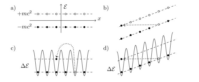
Figure 3: Sketch of the analogy: a) Dirac sea for $E=0$, b) Sauter-Schwinger tunneling for $E\neq 0$, c) Mott state with energy gap $\Delta\cal E$, d) tunneling in tilted lattice.

We can now use this analogy to apply our knowledge of the Sauter-Schwinger effect [76, 77, 78, 79, 80, 81] to particle-hole creation in the tilted Bose-Hubbard model – as Richard Feynman said: The same equations have the same solutions. For example, consider a purely time-dependent electric field of the following form

$$\mathbf{E}=\frac{E_{0}\mathbf{e}_{z}}{\cosh^{2}\left(t/\tau\right)}\,.$$ (72)

Such a profile is called Sauter pulse since F. Sauter was the first to realise (already in 1931) that the Dirac equation and the Klein-Fock-Gordon equation in the presence of such a field can be solved exactly in terms of hypergeometric functions (although he considered the form with $t$ and $x$ interchanged). From the exact solution of the scalar field case, one obtains [82, 83]

$$|\beta_{\mathbf{k}}|^{2}=\frac{\cosh\left(\pi\tau[\omega_{+}-\omega_{-}]\right)+\cosh\left(\pi\sqrt{4E_{0}^{2}c^{2}\tau^{4}-1}\right)}{2\sinh(\pi\tau\omega_{+})\sinh(\pi\tau\omega_{-})}\,,$$ (73)

with the abbreviations

$$\omega_{\pm}=\sqrt{c^{2}(k_{z}\mp E_{0}\tau)^{2}+m_{e}^{2}c^{4}+k_{\perp}^{2}c^{2}}\,.$$ (74)

Here $k_{\perp}$ denotes the momentum perpendicular to the electric field and $m_{e}$ is the mass of the electron. Via the analogy established above, expression (73) yields the momentum dependent particle-hole pair creation probability in a Mott state subject to a time-dependent tilt according to Eq. (72). For various pulse lengths $\tau$, this result plotted in Fig. 14 and compared to numerical results for a one-dimensional Bose-Hubbard lattice.

In the static limit $\tau\rightarrow\infty$, Eq. (73) reproduces the well-known expression

$$|\beta_{\mathbf{k}}|^{2}=\exp\left(-\pi\frac{m_{e}^{2}c^{4}+k_{\perp}^{2}c^{2}}{E_{0}c}\right)\,.$$ (75)

As we see, the electron-positron pair creation probability is exponentially suppressed for small electric fields $E_{0}$. Inserting the translation formula (70) and (71), we get the same exponential suppression for the particle-hole pair creation probability via tunnelling in tilted Mott lattices. Thus, in order to actually verify this prediction experimentally, the tilt should not be too small. In this case, the terms with $\dot{T}_{\mathbf{k}}$ and $\ddot{T}_{\mathbf{k}}$ we have neglected earlier due to $\dot{T}_{\mathbf{k}}=\,{\cal O}(\mathbf{E})$ might start to play a role. Thus, let us estimate the impact of these contributions. Including the terms involving $\dot{T}_{\mathbf{k}}$ and $\ddot{T}_{\mathbf{k}}$, we find

$$\partial_{t}^{2}u_{\mathbf{k}}+\left[m_{\rm eff}^{2}c^{4}_{\rm eff}+k_{\perp}^{2}c^{2}_{\rm eff}+c^{2}_{\rm eff}(k_{z}-E_{0}t)^{2}\right]u_{\mathbf{k}}$$

$$+\xi\left[-E_{0}^{2}+iE_{0}U(k_{z}-E_{0}t)\right]u_{\mathbf{k}} = 0\,,$$ (76)

where we have assumed a constant field ($\tau\rightarrow\infty$) for simplicity. The above differential equation can be solved in terms of parabolic cylindrical functions from which the pair creation probability is determined to be

$$|\beta_{\mathbf{k}}|^{2}\approx\exp\left[-\frac{\pi}{E_{0}c_{\rm eff}}\left(m_{\rm eff}^{2}c^{4}_{\rm eff}+c^{2}_{\rm eff}k_{\perp}^{2}-\xi E_{0}^{2}+\xi^{2}\frac{E_{0}^{2}U^{2}}{4c^{2}_{\rm eff}}\right)\right]\,.$$ (77)

In Fig. 4, we depicted the dependence of the particle-hole creation probability $\langle\hat{p}^{\dagger}_{\mu}\hat{p}_{\mu}\rangle=\sum_{\mathbf{k}}|\beta_{\mathbf{k}}|^{2}/N$ on the potential gradient.

Figure 4: Dependence of $-\ln(\langle\hat{p}^{\dagger}_{\mu}\hat{p}_{\mu}\rangle)$ on the lattice tilt for $J/U=0.1$. The black line represents the standard result (75) for the static Sauter-Schwinger effect while the red curve deviates due to perturbative corrections in $E_{0}$ given by the lattice structure, see equation (77).

9 Second Order in $1/Z$

So far, we have only considered the first order in $1/Z$. Now let us discuss the effect of higher orders by means of few examples. Let us go back to the derivation from (10) to (12) and include $1/Z^{2}$ corrections. To achieve this level of accuracy, we should not replace the exact on-site density matrix $\hat{\rho}_{\mu}$ by it lowest-order approximation $\hat{\rho}_{\mu}^{0}$ but include its first-order corrections in (33), i.e., the quantum depletion $f_{0}=\,{\cal O}(1/Z)$ of the unit filling (Mott) state. This results in a renormalisation of the eigenfrequency

$$\omega_{\mathbf{k}}^{\rm ren}=\sqrt{U^{2}-6JT_{\mathbf{k}}(1-3f_{0})+J^{2}T_{\mathbf{k}}^{2}(1-3f_{0})^{2}}\,,$$ (78)

which indicates a shift of the Mott-superfluid transition to slightly higher values of $J$,

$$J_{\rm crit}^{\rm ren}=U\,\frac{3-2\sqrt{2}}{1-3f_{0}}>U(3-2\sqrt{2})\,,$$ (79)

see Appendix 19. Since the net effect can roughly be understood as a reduction of the effective hopping rate $J^{\rm ren}=J(1-3f_{0})$, it is easy to visualise that this implies also a decrease of the effective propagation velocity.

There are also other $1/Z^{2}$ corrections in (12) such as the three-point correlator $\hat{\rho}^{\rm corr}_{\mu\nu\kappa}$ but they act as source terms and do not affect the eigenfrequency (at second order). However, there are other quantities where these source terms are crucial. In particular we consider correlation functions which are of the form

$$F_{\cal O}(\mu,\nu)=\langle\hat{\cal O}_{\mu}\hat{\cal O}_{\nu}\rangle-\langle\hat{\cal O}_{\mu}\rangle\langle\hat{\cal O}_{\nu}\rangle\;,$$ (80)

and vanish to first order in $1/Z$, in contrast to the off-diagonal long-range order $\langle\hat{a}_{\mu}^{\dagger}\hat{a}_{\nu}\rangle$ discussed above. One important example is the particle-number correlation, i.e., $\langle\hat{n}_{\mu}\hat{n}_{\nu}\rangle-1$. After a somewhat lengthy calculation, we find for the ground state correlations (see Appendix 19)

$$F_{n}(\mu,\nu) = \frac{2}{N^{2}}\sum_{\mathbf{p},\mathbf{q}}e^{i(\mathbf{p}+\mathbf{q})\cdot(\mathbf{x}_{\mu}-\mathbf{x}_{\nu})}\left(f^{11}_{\mathbf{p}}f^{11}_{\mathbf{q}}-f^{12}_{\mathbf{p}}f^{21}_{\mathbf{q}}\right)\,,$$ (81)

where $f^{12}_{\mathbf{p}},f^{21}_{\mathbf{p}}$ and $f^{11}_{\mathbf{p}}$ are given through equations (27) and (28). It is also possible to calculate this quantity via a perturbation expansion into powers of $J/U$. Note, however, that the above result is not perturbative in $J/U$, see, for example, the non-polynomial dependence of $\omega_{\mathbf{k}}$ on $J$.

These predictions could be tested experimentally by site-resolved imaging, i.e., measurements on single lattice sites [10, 84, 85, 86]. In some of these experiments, the particle number per site is not directly measured, but only the parity – i.e., whether the number of particles on a given lattice site is even or odd [19]. The parity correlator reads

$$F_{(-1)^{n}}(\mu,\nu) = \frac{8}{N^{2}}\sum_{\mathbf{p},\mathbf{q}}e^{i(\mathbf{p}+\mathbf{q})\cdot(\mathbf{x}_{\mu}-\mathbf{x}_{\nu})}\left(f^{11}_{\mathbf{p}}f^{11}_{\mathbf{q}}+f^{12}_{\mathbf{p}}f^{21}_{\mathbf{q}}\right)\,.$$ (82)

Again, this result can be compared with a perturbative expansion into powers of $J/U$. Assuming a hyper-cubic lattice ${\mathbb{Z}}^{D}$ in $D$ dimensions with nearest-neighbour hopping (i.e., $Z=2D$), we obtain up to quartic order in $J$

$$F_{(-1)^{n}}(\mu,\nu) = \left(\frac{J}{ZU}\right)^{2}8n(n+1)+$$ (83)

$$+\left(\frac{J}{ZU}\right)^{4}\frac{2n(1+n)}{3}\left[n(n+1)(70-208Z+48Z^{2})+\right.$$

$$\quad\left.+4-22Z+9Z^{2}\right]+\,{\cal O}(J^{6})\,,$$

where $\mu$ and $\nu$ are nearest neighbours and $n=\langle\hat{n}_{\mu}\rangle$ is an arbitrary (integer) filling. Inserting $n=1$ and keeping only the lowest-order $1/Z^{2}$ terms, we may compare this result with (82), after an expansion into powers of $J$, and find perfect agreement.

However, there is an interesting observation regarding the above equation: In one spatial dimension with $Z=2$ nearest neighbours, the $J^{4}$ contribution in the above equation is negative. This suggests that the parity correlator assumes its maximum at a finite value of $J$ (in the Mott phase), which can indeed be confirmed by numerical simulations, see, e.g., [20] and Section 10. In two or more spatial dimensions, the situation is different. Even though the parity correlator should still assume its maximum at some finite value of $J$, this value is quite close to the phase transition or already in the superfluid regime. Thus, this maximum is not visible in our $1/Z$-expansion starting in the Mott state, which predicts a monotonously increasing parity correlation in its region of applicability.

In analogy to Sections 5 and 6, we can also study the correlations after a quantum quench with $J(t)=J\Theta(t)$. Again, there are no contributions to the particle-number and parity correlations in first order $1/Z$ – but, to second order $1/Z$, we find formally the same expressions as in the static case (82) and (81)

$$F_{n}(\mu,\nu) = \frac{2}{N^{2}}\sum_{\mathbf{p},\mathbf{q}}e^{i(\mathbf{p}+\mathbf{q})\cdot(\mathbf{x}_{\mu}-\mathbf{x}_{\nu})}\left(f^{11}_{\mathbf{p}}(t)f^{11}_{\mathbf{q}}(t)-f^{12}_{\mathbf{p}}(t)f^{21}_{\mathbf{q}}(t)\right)\,,$$ (84)

and

$$F_{(-1)^{n}}(\mu,\nu) = \frac{8}{N^{2}}\sum_{\mathbf{p},\mathbf{q}}e^{i(\mathbf{p}+\mathbf{q})\cdot(\mathbf{x}_{\mu}-\mathbf{x}_{\nu})}\left(f^{11}_{\mathbf{p}}(t)f^{11}_{\mathbf{q}}(t)+f^{12}_{\mathbf{p}}(t)f^{21}_{\mathbf{q}}(t)\right)\,,$$ (85)

where $f^{12}_{\mathbf{p}}(t)$,$f^{21}_{\mathbf{p}}(t)$ and $f^{11}_{\mathbf{p}}(t)$ are now given by equations (35) and (36). The parity correlations after a quench have been experimentally observed in a one-dimensional setup [19]. Although the hierarchical expansion relies on a large coordination number, we find qualitative agreement between the theoretical prediction (85) for $Z=2$ and the results from [19]. For large times $t$ and distances $\mathbf{x}_{\mu}-\mathbf{x}_{\nu}$, we may estimate the integrals over $\mathbf{p}$ and $\mathbf{q}$ in the expressions (84) and (85) via the stationary-phase or saddle-point approximation. The dominant contributions stem from the momenta satisfying the saddle-point condition

$$\nabla_{\mathbf{k}}\left[\mathbf{k}\cdot(\mathbf{x}_{\mu}-\mathbf{x}_{\nu})\pm\omega_{\mathbf{k}}t\right]=0\,.$$ (86)

Thus their structure is determined by the group velocity $\mathbf{v}_{\mathbf{k}}=\nabla_{\mathbf{k}}\omega_{\mathbf{k}}$. If the equation $\mathbf{x}_{\mu}-\mathbf{x}_{\nu}=\pm\mathbf{v}_{\mathbf{k}}t$ has a real solution $\mathbf{k}$, i.e., if the distance $\mathbf{x}_{\mu}-\mathbf{x}_{\nu}$ can be covered in the time $t$ with the group velocity $\mathbf{v}_{\mathbf{k}}$, then we get a stationary-phase solution – otherwise the integral will be exponentially suppressed (i.e., the saddle point $\mathbf{k}$ becomes complex). For small values of $J$, the maximum group velocity is given by $\mathbf{v}_{\mathbf{k}}^{\rm max}\approx 3J$, which determines the maximum propagation speed of the correlations, i.e., the effective light-cone.

10 Numerical Simulations for the Bose-Hubbard model

In the following we analyze the Bose-Hubbard system (1) numerically in one and two dimensions. All calculations are carried out on a finite lattice with $L$ lattice sites and $N$ bosons.

10.1 General formalism for the one-dimensional Hubbard model

The eigenstates of lattice systems are calculated by means of exact numerical diagonalisation of the Hamiltonian matrix [87, 88, 89, 90, 91, 92, 93, 94, 95] which can be obtained from the Hamiltonian (1) using the basis of Fock states

$$|{\bf n}_{\Gamma}\rangle=\bigotimes_{\mu=1}^{L}|n_{\Gamma\mu}\rangle\;,\quad\Gamma=1,\dots,{\cal D}\;,\quad{\cal D}=\frac{(N+L-1)!}{N!(L-1)!}\;,$$ (87)

where $\Gamma$ labels the configuration of the bosons and the occupation numbers of individual lattice sites $n_{\Gamma\mu}$ satisfy the condition

$$N=\sum_{\mu=1}^{L}n_{\Gamma\mu}\;.$$ (88)

The matrix dimension can be reduced by factor $L$ for homogeneous lattices with periodic boundary conditions ($\hat{b}_{L+1}\equiv\hat{b}_{1}$). In this case the Hamiltonian commutes with the unitary translation operator $\hat{\cal T}$ which acts through cyclic permutation on the lattice bosons. Due to the periodic boundary conditions, the operator satisfies $\hat{{\cal T}}^{L}=1$. As a basis one can use linear combinations of the Fock states (87) in the form

$$|{\bf n}_{K\Gamma}\rangle={\cal N}_{\Gamma}\sum_{\mu=1}^{L}\left(\frac{\hat{\cal T}}{\tau_{K}}\right)^{\mu-1}|{\bf n}_{\Gamma}\rangle\;,$$ (89)

which are eigenstates of the operator $\hat{{\cal T}}$ for the eigenvalue $\tau_{K}=\exp\left(iK\right)$. ${\cal N}_{\Gamma}$ are normalisation constants chosen such that $\langle{\bf n}_{K\Gamma}|{\bf n}_{K^{\prime}\Gamma^{\prime}}\rangle=\delta_{\Gamma\Gamma^{\prime}}\delta_{KK^{\prime}}$. Here the state $|{\bf n}_{\Gamma}\rangle$ cannot be obtained by cyclic permutations of $|{\bf n}_{\Gamma^{\prime}}\rangle$ with $\Gamma^{\prime}\neq\Gamma$. The eigenstates of the Hamiltonian have the following form

$$|K\Omega\rangle=\sum_{\Gamma=1}^{{\cal D}_{K}}C_{K\Omega\Gamma}|{\bf n}_{K\Gamma}\rangle\;,\quad\Omega=1,\dots,{\cal D}_{K}\;,\quad\sum_{K=0}^{L-1}{\cal D}_{K}={\cal D}\;,$$ (90)

and the corresponding eigenenergies are denoted by $E_{K\Omega}$.

If the complete eigenvalue problem is solved, one can work out expectation value of any operator $\hat{\cal O}$ at arbitrary temperature in a canonical ensemble as

$$\langle\hat{\cal O}\rangle_{T}=\frac{1}{{\cal Z}(T)}\sum_{K\Omega}\langle K\Omega|\hat{\cal O}|K\Omega\rangle\exp\left(-\frac{E_{K\Omega}}{T}\right)$$ (91)

with the partition function

$${\cal Z}(T)=\sum_{K\Omega}\exp\left(-\frac{E_{K\Omega}}{T}\right)\;.$$ (92)

Using the set of the basis states (89) we were able to solve numerically the complete eigenvalue problem for $N=L=9$.

In order to study zero-temperature properties of the system, it is sufficient to calculate the ground state. This can be done exactly with the aid of iterative numerical solvers for sparse matrices of large dimensions along the lines of [91]. We were able to do this up to $N=L=14$.

10.2 Energy spectrum

In the limit of vanishing hopping, $J=0$, the basis states (89) are the eigenstates of the Hamiltonian (1) which are, apart from the ground state, degenerate. The ground state has equal occupation numbers at each lattice site, that is $n_{\Gamma\mu}\equiv n$. It exists only at $K=0$ and has the energy

$$E_{01}=L\frac{U}{2}n(n-1)\,.$$ (93)

The energy eigenvalues of the degenerated excited states are given through

$$E_{K\Gamma}=\sum_{\mu=1}^{L}\frac{U}{2}n_{\Gamma\mu}\left(n_{\Gamma\mu}-1\right)$$ (94)

and do not depend on $K$, corresponding to flat energy bands. The lowest band contains $L(L-1)$ degenerate eigenstates with the energies $E_{K\Gamma}=E_{01}+U$. These states correspond to bosonic configurations with the same occupation numbers $n$ at any site except two, one of which contains $n-1$ boson and the other one $n+1$. The highest band contains $L$ degenerate states with all atoms sitting at one lattice site. These states have the energy $E_{K\Gamma}=UN(N-1)/2$. A finite hopping rate $J$ lifts the degeneracy, the bands aquire finite widths and can even overlap if the tunneling parameter is large enough.

The full energy spectrum calculated for $N=L=9$ and $J/U=0.1$, which corresponds to the Mott-insulator state, is shown in Fig. 5(a). The lowest dot at $K=0$ is the ground state energy $E_{01}$, see also Fig. 5(b). Also the lowest excited state is located at $K=0$ and has the energy $E_{02}$. Together with the energies $E_{K2}$, where $K\neq 0$, they form the lowest excitation branch shown by the black lines in Figs. 5(b,c). An increase of the system size leads to more dense distribution of the points and the solid line becomes smoother. We see that, at small momenta $K$, the lowest excitation branch can be approximated by a pseudo-relativistic form

$$\omega_{\bf K}^{2}\equiv(E_{K2}-E_{01})^{2}=(\Delta{\cal E})^{2}+K^{2}v_{\rm eff}^{2}\;.$$ (95)

Thus we can estimate the effective velocity $v_{\rm eff}$ using the numerically calculated values of $E_{01}$, $E_{02}$ and $E_{11}$. The results for different system sizes are shown in Fig. 5(d). With the increase of $J/U$ the energy bands become broader and the gap in the excitation spectrum $E_{02}-E_{01}$ becomes smaller.

The energy eigenvalues in the lowest band in Fig. 5 correspond to particle-hole excitations of the form $\hat{p}^{\dagger}_{k_{p}}\hat{h}_{k_{h}}|\Psi_{\mathrm{Mott}}\rangle$ with the total momentum $k_{p}+k_{h}=K$. When discussing the ground-state properties or the dynamics after a quench in the previous Sections, it was sufficient to consider translationally invariant states with $K=0$, i.e., $k_{p}=-k_{h}=k$, where $k$ corresponds to the relative momentum. In the discussion of the Sauter-Schwinger analogue, we considered a spatially constant potential gradient and absorbed it into the Fourier coefficients $T_{\mathbf{k}}(t)$ via a Peierls transformation, finally arriving at the evolution equations (59) and (60) for particle and hole operators with $k_{p}=-k_{h}=k$. However, for arbitrary potentials $V_{\mu}$, this is no longer possible in this simple form. In order to satisfy the equations of motion (19-21) for the correlation functions for an arbitrary potential $V_{\mu}$, one should employ the generalised evolution equations

$$\left(i\partial_{t}-V_{\mu}+\frac{U}{2}\right)\hat{h}_{\mu} = \frac{J}{Z}\sum_{\kappa}T_{\mu\kappa}\left(\hat{h}_{\kappa}+\sqrt{2}\hat{p}_{\kappa}\right)\,,$$ (96)

$$\left(i\partial_{t}-V_{\mu}-\frac{U}{2}\right)\hat{p}_{\mu} = -\frac{\sqrt{2}J}{Z}\sum_{\kappa}T_{\mu\kappa}\left(\hat{h}_{\kappa}+\sqrt{2}\hat{p}_{\kappa}\right)\,.$$ (97)

Here the particle and hole-operators are fixed up to a $k_{h,p}$-independent phase. For the limiting case $V_{\mu}\to 0$ we find from Eqs. (96) and (97) the following eigenfrequencies

$$\omega^{h}_{k_{h}} = -\frac{1}{2}(JT_{k_{h}}+\omega_{k_{h}})\,,$$ (98)

$$\omega^{p}_{k_{p}} = -\frac{1}{2}(JT_{k_{p}}-\omega_{k_{p}})\,,$$ (99)

where $\omega_{k}$ are the eigenfrequencies defined in (31). These excitations define the lowest band with the energies

$$E_{K\Omega}=\omega^{p}_{k_{p}}-\omega^{h}_{k_{h}}\,,$$ (100)

where $k_{h}+k_{p}=K$. The spectrum is depicted in Fig. 6 and the effective velocity reads

$$v_{\mathrm{eff}}=\frac{1}{2}\sqrt{J(3U-J)}$$ (101)

which has for $J/U=0.1$ the numerical value $v_{\mathrm{eff}}/U=0.269$. Including the second order corrections in $1/Z^{2}$ we have a slightly lower value $v_{\mathrm{eff}}/U=0.264$, compare Fig. 5(d).

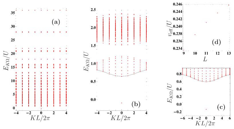
Figure 5: (a) Full energy spectrum and (b) its lowest part for $N=L=9$. (c) Lowest part of the spectrum for $N=L=13$. (d) Effective velocity in a one-dimensional lattice with $n=1$ atom per site and $J/U=0.1$.

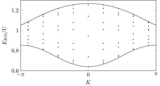
Figure 6: Boundaries of the lowest energy excitation band in the continuum limit (solid lines) and energy excitations for $L=9$ (points) from Eq. (100) in a one-dimensional lattice with $n=1$ and $J/U=0.1$.

10.3 Probability distribution of the occupation numbers

We calculate the ground state and then the probabilities $p(n_{\mu})$ to have $n_{\mu}$ atoms at a lattice site which satisfy the normalisation condition

$$\sum_{n_{\mu}=0}^{N}p(n_{\mu})=1\;.$$ (102)

As in the previous Section, we consider the system with $N=L$. From Eqs. (3) and (4) it follows that in the limit $J=0$ we have $p(n_{\mu})=\delta_{n_{\mu},1}$, and in the opposite limit $U=0$ the probabilities are given by the binomial distribution

$$p(n_{\mu})=\frac{N!}{(N-n_{\mu})!n_{\mu}!}\left(\frac{1}{N}\right)^{n_{\mu}}\left(1-\frac{1}{N}\right)^{N-n_{\mu}}\;.$$ (103)

The result for $N=14$ at arbitrary $J/U$ and at zero temperature is shown in Fig. 7. One can clearly see that the probability to have three particles or more at one lattice site is very small which is consistent with the approximations used in the $1/Z$ expansion.

The particle-number distribution at finite temperature is shown in Fig. 8(b). Comparison with the zero-temperature result for the same system size [Fig. 8(a)] indicates that temperature has stronger influence at smaller values of $J/U$.

\psfrag{J}[c]{$J/U$}\psfrag{p}[b]{$p(n_{\mu})$}\includegraphics[width=199.16928pt]{p1D-N_14-L_14-Z.eps}

Figure 7: Probabilities to have $n_{\mu}=0$ (red), $1$ (green), $2$ (blue), $3$ (magenta) atoms at a lattice site in a one-dimensional lattice of $L=14$ sites with $n=1$ atom per site at zero temperature.

\psfrag{J}[c]{$J/U$}\psfrag{p}[b]{$p(n_{\mu})$}\psfrag{a}[c]{\bf(a)}\includegraphics[width=199.16928pt]{p1D-N_9-L_9-Z.eps}

\psfrag{J}[c]{$J/U$}\psfrag{p}[b]{$p(n_{\mu})$}\psfrag{a}[c]{\bf(a)}\psfrag{b}[c]{\bf(b)}\includegraphics[width=199.16928pt]{p1D-N_9-L_9-T_0.3-Z.eps}

\psfrag{J}[c]{$J/U$}\psfrag{p}[b]{$p(n_{\mu})$}\psfrag{a}[c]{\bf(a)}\psfrag{b}[c]{\bf(b)}\psfrag{a}[c]{\bf(c)}\includegraphics[width=199.16928pt]{p2D-N_9-L_9-Z.eps}

\psfrag{J}[c]{$J/U$}\psfrag{p}[b]{$p(n_{\mu})$}\psfrag{a}[c]{\bf(a)}\psfrag{b}[c]{\bf(b)}\psfrag{a}[c]{\bf(c)}\psfrag{b}[c]{\bf(d)}\includegraphics[width=199.16928pt]{p2D-N_9-L1_3-L2_3-T_0.3-Z.eps}

Figure 8: Probabilities to have $n_{\mu}=0$ (red), $1$ (green), $2$ (blue), $3$ (magenta) atoms at a site in a lattice with $n=1$ atom per site. (a) and (b): one-dimensional lattice of $L=9$ sites; (c) and (d): two-dimensional lattice of $3\times 3$ sites; (a) and (c): zero temperature; (b) and (d): $T/U=0.3$.

10.4 Two-point correlation functions

In this Subsection, we consider two-point correlation functions which have been discussed in Section 9. Due to the translational invariance, the correlation functions depend on the distance $s=|x_{\mu}-x_{\nu}|$ and have the property $F_{\cal O}(\mu,\nu)=F_{\cal O}(s)=F_{\cal O}(L-s)$ in view of the periodic boundary conditions.

First we consider the parity correlation function $F_{(-1)^{n}}(s)$. Its dependence on $J/U$ as well as on the distance $s$ is shown in Fig. 9. This result is in a very good quantitative agreement with the DMRG-calculations [20]. Note that our definition of $J$ differs by a factor $Z$ from that used in [20]. Fig. 9 shows the number correlation function $F_{n}(s)$.

\psfrag{J}[c]{$J/U$}\psfrag{par}[b]{$F_{(-1)^{n}}(s)$}\psfrag{a}[c]{\bf(a)}\includegraphics[width=199.16928pt]{par1D-N_14-L_14-Z.eps}

\psfrag{J}[c]{$J/U$}\psfrag{par}[b]{$F_{(-1)^{n}}(s)$}\psfrag{a}[c]{\bf(a)}\psfrag{n}[c]{$s$}\psfrag{b}[c]{\bf(b)}\includegraphics[width=199.16928pt]{par1Dlog-J_0.05-N_14-L_14.eps}

\psfrag{J}[c]{$J/U$}\psfrag{par}[b]{$F_{(-1)^{n}}(s)$}\psfrag{a}[c]{\bf(a)}\psfrag{n}[c]{$s$}\psfrag{b}[c]{\bf(b)}\psfrag{J}[c]{$J/U$}\psfrag{dd}[b]{$F_{n}(s)$}\psfrag{a}[c]{\bf(c)}\includegraphics[width=199.16928pt]{dd1D-N_14-L_14-Z.eps}

\psfrag{J}[c]{$J/U$}\psfrag{par}[b]{$F_{(-1)^{n}}(s)$}\psfrag{a}[c]{\bf(a)}\psfrag{n}[c]{$s$}\psfrag{b}[c]{\bf(b)}\psfrag{J}[c]{$J/U$}\psfrag{dd}[b]{$F_{n}(s)$}\psfrag{a}[c]{\bf(c)}\psfrag{n}[c]{$s$}\psfrag{ddm1}[b]{$\left|F_{n}(s)\right|$}\psfrag{b}[c]{\bf(d)}\includegraphics[width=199.16928pt]{dd1Dlog-J_0.05-N_14-L_14.eps}

Figure 9: Parity correlation [(a) and (b)] and density-density correlation [(c) and (d)] in a one-dimensional lattice of $L=14$ sites with $n=1$ atom per site at zero temperature. (a) and (c): dependence on $J/U$ for $s=1$ (red), $2$ (green), $3$ (blue), $4$ (magenta); (b) and (d): Dependence on $s$ for $J/U=0.1$. Due to the periodic boundary conditions correlation functions increase starting from $s=7$.

Fig. 10 shows matrix elements of the one-body density matrix $\langle\hat{b}_{\mu}^{\dagger}\hat{b}_{\mu+s}\rangle$ as well as its momentum distribution (38). In a finite lattice the quasi-momentum takes discrete values which are integer multiples of $2\pi/L$. These allowed values are marked in Fig. 10(a) by dots. The momentum distribution calculated in the first order of $1/Z$ is also shown for comparison. We observe good quantitative agreement.

\psfrag{k}[c]{$k$}\psfrag{pdis}[b]{$P(k)$}\psfrag{b}[c]{\bf(b)}\psfrag{a}[c]{\bf(a)}\includegraphics[width=199.16928pt]{md1D-J_0.05-N_14-L_14.eps}

\psfrag{k}[c]{$k$}\psfrag{pdis}[b]{$P(k)$}\psfrag{b}[c]{\bf(b)}\psfrag{a}[c]{\bf(a)}\psfrag{dm}[b]{$\langle\hat{b}_{\mu}^{\dagger}\hat{b}_{\mu+s}\rangle$}\psfrag{n}[c]{$s$}\includegraphics[width=199.16928pt]{obdm1Dlog-J_0.05-N_14-L_14.eps}

Figure 10: (a): Momentum distribution (38) in a one-dimensional lattice with $n=1$ atom per site at $J/U=0.1$ and zero temperature. The result obtained by exact diagonalisation for a finite lattice of $L=14$ is shown by dots. The solid line is a calculation in the first order of $1/Z$ for an infinite lattice. (b): Correlation function $\langle\hat{b}_{\mu}^{\dagger}\hat{b}_{\mu+s}\rangle$ calculated by exact diagonalisation for a finite lattice with the same values of parameters as in (a).

10.5 Particle-number distribution and correlation functions in 2D

The whole procedure of exact numerical diagonalisation described for one-dimensional systems can be generalised to higher dimensions. We did numerical simulations for two-dimensional square lattices of $3\times 3$ lattice sites with periodic boundary conditions. Exact calculations for square lattices of the size $4\times 4$ and larger were not possible due to the problem with computer memory. Due to the fact that the size of the two-dimensional system is very small one can expect strong finite-size effects. However, as we will see later numerical calculations give qualitatively correct predictions valid for large systems.

The probability distribution of the occupation numbers is shown in Figs. 8(c) and (d). It is very similar to the one-dimensional case. In a lattice of $3\times 3$ sites with periodic boundary conditions the distance $s$ takes only three values $s=0,1,\sqrt{2}$ which makes the study of the long-range behavior of the two-point correlation functions practically impossible. Nevertheless some useful information can be obtained in the Mott-insulator phase where the correlations decay exponentially. Fig. 11(a) shows the dependence of the parity correlation function on $J/U$. As in the one-dimensional case, $F_{(-1)^{n}}(s)$ has a maximum at a finite value of $J$, which is, however, not in the Mott phase. The results in Fig. 11 are in a good agreement with those obtained in [20] by DMRG and MPS calculations for large systems. Correlations $\langle\hat{n}_{\mu}\hat{n}_{\nu}\rangle$ and $\langle\hat{b}_{\mu}^{\dagger}\hat{b}_{\nu}\rangle$ are shown in Figs. 11(b), 11(c), respectively. They become stronger for increasing values of $J/U$.

\psfrag{J}[c]{$J/U$}\psfrag{par}[b]{$F_{(-1)^{n}}(s)$}\psfrag{a}[c]{\bf(a)}\includegraphics[width=199.16928pt]{par2D-N_9-L1_3-L2_3-Z.eps}

\psfrag{J}[c]{$J/U$}\psfrag{par}[b]{$F_{(-1)^{n}}(s)$}\psfrag{a}[c]{\bf(a)}\psfrag{J}[c]{$J/U$}\psfrag{dd}[b]{$F_{n}(s)$}\psfrag{b}[c]{\bf(b)}\includegraphics[width=199.16928pt]{dd2D-N_9-L1_3-L2_3-Z.eps}

\psfrag{J}[c]{$J/U$}\psfrag{dm}[b]{$\langle\hat{b}_{\mu}^{\dagger}\hat{b}_{\nu}\rangle$}\psfrag{c}[c]{\bf(c)}\includegraphics[width=199.16928pt]{obdm2D-N_9-L1_3-L2_3-Z.eps}

Figure 11: Parity correlation (a), density-density correlation (b) and elements of the one-body density matrix (c) in a two-dimensional lattice of $3\times 3$ sites with $n=1$ atom per site at zero temperature. $s=1$ (red), $\sqrt{2}$ (green).

10.6 Time evolution after quench

If the complete set of the eigenvalues and eigenstates of the Hamiltonian is known, the time evolution of an arbitrary initial state $|\psi(0)\rangle$ can be calculated exactly without numerical integration, provided that the Hamiltonian does not depend explicitly on time. The initial state can be decomposed into the eigenstates of the Hamiltonian as

$$|\psi(0)\rangle=\sum_{K}\sum_{\Omega=1}^{{\cal D}_{K}}c_{K\Omega}|K\Omega\rangle\;,\quad c_{K\Omega}=\langle\psi(0)|K\Omega\rangle\;.$$ (104)

If the parameters of the Hamiltonian do not depend on time, the evolution of the initial state is given by

$$|\psi(t)\rangle=\sum_{K}\sum_{\Gamma=1}^{{\cal D}_{K}}c_{K\Gamma}(t)|{\bf n}_{K\Gamma}\rangle$$ (105)

with

$$c_{K\Gamma}(t)=\sum_{\Omega=1}^{{\cal D}_{K}}c_{K\Omega}C_{K\Omega\Gamma}\exp\left(-iE_{K\Omega}t\right)\;.$$ (106)

The time dependence of the expectation value of any operator $\hat{\cal O}$ can be calculated as

$$\langle\hat{\cal O}\rangle(t)=\sum_{K\Gamma}\sum_{K^{\prime}\Gamma^{\prime}}\langle{\bf n}_{K\Gamma}|\hat{\cal O}|{\bf n}_{K^{\prime}\Gamma^{\prime}}\rangle c_{K\Gamma}^{*}(t)c_{K^{\prime}\Gamma^{\prime}}(t)\;.$$ (107)

We will be dealing with operators $\hat{\cal O}$ which have the property

$$\langle{\bf n}_{K\Gamma}|\hat{\cal O}|{\bf n}_{K^{\prime}\Gamma^{\prime}}\rangle=\langle{\bf n}_{K\Gamma}|\hat{\cal O}|{\bf n}_{K\Gamma^{\prime}}\rangle\delta_{KK^{\prime}}\;.$$ (108)

Then the expectation value averaged over the evolution time is given by

$$\overline{\langle\hat{\cal O}\rangle} = \lim_{t\to\infty}\frac{1}{t}\int_{0}^{t}\langle\hat{\cal O}\rangle(t^{\prime})dt^{\prime}$$ (109)

$$= \sum_{K}\sum_{\Gamma}\sum_{\Gamma^{\prime}}\langle{\bf n}_{K\Gamma}|\hat{\cal O}|{\bf n}_{K\Gamma^{\prime}}\rangle\sum_{\Omega=1}^{{\cal D}_{K}}\left|c_{K\Omega}\right|^{2}C^{*}_{K\Omega\Gamma}C_{K\Omega\Gamma^{\prime}}\;.$$

We study time evolution of the initial state with exactly one atom at each lattice site which is the ground state with $K=0$ of the Bose-Hubbard Hamiltonian in the limit $J=0$. Since the Hamiltonian after quench preserves the translational invariance, the time evolution involves only states with $K=0$. In Figs. 12 and 13 we present numerical results for the particle-number distribution $p(n_{\mu})$ and correlation function $\langle\hat{b}_{\mu}^{\dagger}\hat{b}_{\nu}\rangle$ in one and two dimensions. The purpose of this study is to address the question of (quasi) equilibration versus thermalisation in closed quantum systems. Time evolution of the probabilities $p(n_{\mu})$ for one- and two-dimensional systems is shown in Figs. 12(a), 13(a), respectively. On large time scales they oscillate around the averaged values shown by straight horizontal lines. For the chosen value of $J/U=0.1$, the behavior $p(0)$ is almost indistinguishable from that of $p(2)$. Figs. 12(b), 13(b) show the dependence of the probabilities on the temperature. Averaged values of the probabilities correspond to the effective temperature which is slightly less than $0.15~{}U$.

\psfrag{t}[c]{$tU$}\psfrag{Pn}[b]{$p(n_{\mu})$}\psfrag{a}[c]{\bf(a)}\includegraphics[width=199.16928pt]{pn1Dt-J_0.05-N_9-L_9-NC_9.eps}

\psfrag{t}[c]{$tU$}\psfrag{Pn}[b]{$p(n_{\mu})$}\psfrag{a}[c]{\bf(a)}\psfrag{T}[c]{$T/U$}\psfrag{b}[c]{\bf(b)}\includegraphics[width=199.16928pt]{pn1DT-J_0.05-N_9-L_9-NC_9.eps}

\psfrag{t}[c]{$tU$}\psfrag{Pn}[b]{$p(n_{\mu})$}\psfrag{a}[c]{\bf(a)}\psfrag{T}[c]{$T/U$}\psfrag{b}[c]{\bf(b)}\psfrag{OBDM}[b]{$\langle\hat{b}_{\mu}^{\dagger}\hat{b}_{\mu+s}\rangle$}\psfrag{t}[c]{$tU$}\psfrag{a}[c]{\bf(c)}\includegraphics[width=199.16928pt]{obdm1Dt-J_0.05-N_9-L_9-NC_9.eps}

\psfrag{t}[c]{$tU$}\psfrag{Pn}[b]{$p(n_{\mu})$}\psfrag{a}[c]{\bf(a)}\psfrag{T}[c]{$T/U$}\psfrag{b}[c]{\bf(b)}\psfrag{OBDM}[b]{$\langle\hat{b}_{\mu}^{\dagger}\hat{b}_{\mu+s}\rangle$}\psfrag{t}[c]{$tU$}\psfrag{a}[c]{\bf(c)}\psfrag{T}[c]{$T/U$}\psfrag{b}[c]{\bf(d)}\includegraphics[width=199.16928pt]{obdm1DT-J_0.05-N_9-L_9-NC_9.eps}

Figure 12: Quench and (quasi) equilibration in a one-dimensional lattice of $L=9$ sites with $n=1$ atom per site. (a) Time evolution of the probabilities to have $n_{\mu}=0$ (red), $2$ (blue) atoms at a lattice site after quench $J/U=0\to 0.1$. (b) Probabilities to have $n_{\mu}=0$ (red), $2$ (blue) atoms at a lattice site for $J/U=0.1$ as a function of temperature. Straight horizontal lines in both panels show the values of probabilities averaged over the infinite evolution time. (c) Elements of the one-body density matrix with $s=1$ (red), $2$ (green), after quench $J/U=0\to 0.1$. (d) Elements of the one-body density matrix with $s=1$ (red), $2$ (green), for $J/U=0.1$ as a function of temperature.

The time dependence of the correlation functions $\langle\hat{b}_{\mu}^{\dagger}\hat{b}_{\nu}\rangle$ presented in Figs. 12(c), 13(c) displays the same oscillating character. In the one-dimensional system, the effective temperature corresponding to the averaged values of $\langle\hat{b}_{\mu}^{\dagger}\hat{b}_{\nu}\rangle$ can be defined but appears to be higher than that of the probabilities $p(n_{\mu})$. In contrast, in the two-dimensional case, the correlation functions $\langle\hat{b}_{\mu}^{\dagger}\hat{b}_{\nu}\rangle$ cannot be described by a thermal state, see Fig. 13(d). The absence of effective temperature in the two-dimensional system is consistent with the result obtained within the $1/Z$ expansion in Section 6.

\psfrag{t}[c]{$tU$}\psfrag{Pn}[b]{$p(n_{\mu})$}\psfrag{a}[c]{\bf(a)}\includegraphics[width=199.16928pt]{pn2Dt-J_0.025-N_9-L1_3-L2_3-NC_9.eps}

\psfrag{t}[c]{$tU$}\psfrag{Pn}[b]{$p(n_{\mu})$}\psfrag{a}[c]{\bf(a)}\psfrag{T}[c]{$T/U$}\psfrag{b}[c]{\bf(b)}\includegraphics[width=199.16928pt]{pn2DT-J_0.025-N_9-L1_3-L2_3-NC_9.eps}

\psfrag{t}[c]{$tU$}\psfrag{Pn}[b]{$p(n_{\mu})$}\psfrag{a}[c]{\bf(a)}\psfrag{T}[c]{$T/U$}\psfrag{b}[c]{\bf(b)}\psfrag{OBDM}[b]{$\langle\hat{b}_{\mu}^{\dagger}\hat{b}_{\nu}\rangle$}\psfrag{t}[c]{$tU$}\psfrag{a}[c]{\bf(c)}\includegraphics[width=199.16928pt]{obdm2Dt-J_0.025-N_9-L1_3-L2_3-NC_9.eps}

\psfrag{t}[c]{$tU$}\psfrag{Pn}[b]{$p(n_{\mu})$}\psfrag{a}[c]{\bf(a)}\psfrag{T}[c]{$T/U$}\psfrag{b}[c]{\bf(b)}\psfrag{OBDM}[b]{$\langle\hat{b}_{\mu}^{\dagger}\hat{b}_{\nu}\rangle$}\psfrag{t}[c]{$tU$}\psfrag{a}[c]{\bf(c)}\psfrag{T}[c]{$T/U$}\psfrag{b}[c]{\bf(d)}\includegraphics[width=199.16928pt]{obdm2DT-J_0.025-N_9-L1_3-L2_3-NC_9.eps}

Figure 13: Quench and (quasi) equilibration in a two-dimensional lattice of $3\times 3$ sites with $n=1$ atom per site. (a) Probabilities to have $n_{\mu}=0$ (red), $2$ (blue) atoms at a lattice site after quench $J/U=0\to 0.1$. (b) Probabilities to have $n_{1}=0$ (red), $2$ (blue) atoms at a lattice site for $J/U=0.1$ as a function of temperature. (c) Elements of the one-body density matrix with $s=1$ (red), $\sqrt{2}$ (green) after quench $J/U=0\to 0.1$. (d) Elements of the one-body density matrix with $s=1$ (red), $\sqrt{2}$ (green) for $J/U=0.1$ as a function of temperature.

10.7 Tilt in one dimension

In this Section, we calculate the probability to create a particle-hole excitation due to the time-dependent tilt. Initial state of the system $|\psi(0)\rangle$ is the ground state of the Hamiltonian (1) for finite value of $J/U$ in the Mott-insulator phase. During the time evolution the system is described by the Hamiltonian (52) with the on-site energies

$$V_{\mu}=E_{0}f(t/\tau)x_{\mu}\;,$$ (110)

where function $f(s)$ has similar form as (72)

$$f(s)=\left\{\cosh^{-2}\left(s-\frac{5}{2}\right)-\cosh^{-2}\left(\frac{5}{2}\right)\right\}\left[1-\cosh^{-2}\left(\frac{5}{2}\right)\right]^{-1}\,,$$ (111)

with $0<s<5$, such that $f(0)=f(5)=0$ and $f(5/2)=1$.

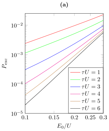
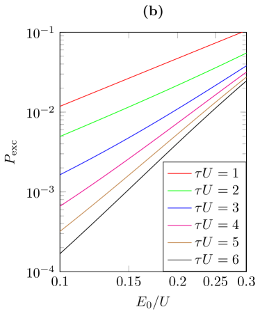
Figure 14: a) Numerical results for the excitation probability per unit time in logarithmic scales for $N=L=12$ and $J/U=0.1$. b) Analytical results (73) for the excitation probability per unit time where the expressions for the effective mass (71) and the effective velocity (70) have been used.

In contrast to all the previous numerical calculation we do not impose anymore periodic boundary conditions. Instead of that we consider the case when the particles cannot tunnel between the lattice sites $\mu=1$ and $\mu=L$ and perform calculations using the basis of Fock states (87). Numerical integration of the Schrödinger equation is done by means of the fourth-order Runge-Kutta method. The accuracy of the numerical integration is controlled by the conservation of norm of the state $|\psi(t)\rangle$.

The results for the excitation probability per unit time

$$P_{\rm exc}=\frac{1-\left|\langle\psi(0)|\psi(5\tau)\rangle\right|^{2}}{\tau}\;,$$ (112)

where $5\tau$ is the total evolution time, are shown in Fig. 14(a). At short evolution times, the excitation probability $P_{\rm exc}$ has a power-law dependence on $\Delta\epsilon$ which corresponds to the perturbative regime of the pair production. One should keep in mind that finite-size effects start to play an important role if the evolution time exceeds $L/v_{\rm eff}$, where $v_{\rm eff}$ is an effective velocity for the propagation of excitations discussed in Section 10.2. For $L=N=12$ and $J/U=0.1$ this leads to the requirement $\tau U<7$. At much longer times $\tau$, the dynamics of a finite-size system will be adiabatic and the excitation probability will tend to zero in contrast to the infinite system, where the excitation probability remains finite in the limit $\tau\rightarrow\infty$ as determined by Eq. (75).

In Fig. 14(b) we show the results of the same calculations obtained in Section 8 in the first order of the $1/Z$-expansion where corrections due to time-derivatives of $T_{\mathbf{k}}$ have been neglected, see Eq. (8). The excitation probability (112) and the particle-hole creation rate are related via

$$P_{\rm exc}=\frac{1-\langle\Psi_{\mathrm{Mott}}|\hat{\rho}(\infty)|\Psi_{\mathrm{Mott}}\rangle}{\tau}\approx\frac{1-(1-2\langle\hat{p}^{\dagger}_{\mu}\hat{p}_{\mu}\rangle)^{N}}{\tau}\approx 2N\frac{\langle\hat{p}^{\dagger}_{\mu}\hat{p}_{\mu}\rangle}{\tau}\;,$$ (113)

where $\langle\hat{p}^{\dagger}_{\mu}\hat{p}_{\mu}\rangle=\sum_{\bf k}\left|\beta_{\bf k}\right|^{2}/N$ and $\beta_{\mathbf{k}}$ is the Bogoliubov coefficient defined in equation (73). We observe a very good qualitative agreement with the results of exact numerical calculations, although the latter give somewhat smaller values of $P_{\rm exc}$.

11 Fermi-Hubbard Model

Now, after having studied the bosonic case, let us investigate the Fermi-Hubbard model [1, 12, 96]. We shall find many similarities to the Bose-Hubbard model – but also crucial differences. The Hamiltonian is given by

$$\hat{H}=-\frac{J}{Z}\sum_{\mu\nu,s}T_{\mu\nu}\hat{c}_{\mu,s}^{\dagger}\hat{c}_{\nu,s}+U\sum_{\mu}\hat{n}_{\mu}^{\uparrow}\hat{n}_{\mu}^{\downarrow}\,.$$ (114)

The nomenclature is the same as in the bosonic case (1) but with an additional spin label $s$ which can assume two values $s=\uparrow$ or $s=\downarrow$. In the following, we consider the case of half-filling $\langle\hat{n}_{\mu}^{\uparrow}+\hat{n}_{\mu}^{\downarrow}\rangle=1$ where half the particles are in the $s=\uparrow$ state and the other have $s=\downarrow$. Note that the total particle numbers $\hat{N}^{\uparrow}=\sum_{\mu}\hat{n}_{\mu}^{\uparrow}$ and $\hat{N}^{\downarrow}=\sum_{\mu}\hat{n}_{\mu}^{\downarrow}$ for each spin species are conserved separately $[\hat{H},\hat{N}^{\uparrow}]=[\hat{H},\hat{N}^{\downarrow}]=0$. The creation and annihilation operators satisfy the fermionic anti-commutation relations

$$\left\{\hat{c}_{\nu,a},\hat{c}_{\mu,b}^{\dagger}\right\}=\delta_{\mu\nu}\delta_{ab}\;,\,\left\{\hat{c}_{\nu,a},\hat{c}_{\mu,b}\right\}=\left\{\hat{c}_{\nu,a}^{\dagger},\hat{c}_{\mu,b}^{\dagger}\right\}=0\,.$$ (115)

The fermionic nature of the particles has important consequences. For example, let us estimate the expectation value of the hopping Hamiltonian $\hat{H}_{J}$. Introducing the “coarse-grained” operator

$$\hat{c}_{\mu,s}^{\Sigma}=\frac{1}{\sqrt{Z}}\sum_{\nu}T_{\mu\nu}\hat{c}_{\nu,s}\,,$$ (116)

we may write the expectation value of the tunnelling energy $\hat{H}_{J}$ per lattice site for one spin species $s$ as $-J\langle\hat{c}_{\mu,s}^{\dagger}\hat{c}_{\mu,s}^{\Sigma}\rangle/\sqrt{Z}$. This expectation value can be interpreted as a scalar product of the two vectors $\hat{c}_{\mu,s}\left|\Psi\right>$ and $\hat{c}_{\mu,s}^{\Sigma}\left|\Psi\right>$ and hence it is bounded by

$$\left|\left<\Psi\right|\hat{c}_{\mu,s}^{\dagger}\hat{c}_{\mu,s}^{\Sigma}\left|\Psi\right>\right|\leq||\hat{c}_{\mu,s}\left|\Psi\right>||\cdot||\hat{c}_{\mu,s}^{\Sigma}\left|\Psi\right>||\,.$$ (117)

Inserting $||\hat{c}_{\mu,s}\left|\Psi\right>||^{2}=\left<\Psi\right|\hat{c}_{\mu,s}^{\dagger}\hat{c}_{\mu,s}\left|\Psi\right>=\left<\Psi\right|\hat{n}_{\mu,s}\left|\Psi\right>$, we get the expectation value of the number operator $\hat{n}_{\mu,s}$. In contrast to the bosonic case, this operator is bounded and thus we find $||\hat{c}_{\mu,s}\left|\Psi\right>||\leq 1$. Furthermore, the operator $\hat{c}_{\mu,s}^{\Sigma}$ in (116) obeys the same anti-commutation relations (115) and thus we find $||\hat{c}_{\mu,s}^{\Sigma}\left|\Psi\right>||\leq 1$ in complete analogy. Consequently, the absolute value of the tunnelling energy per lattice site is below $2J/\sqrt{Z}$, i.e., decreases for large $Z$.

The above result implies that the interaction term $\propto U$ always dominates (except in the trivial case $U=0$) in the limit $Z\to\infty$ under consideration. Hence, we are in the strongly interacting Mott regime and do not find anything analogous to the Mott–superfluid transition as in the bosonic case. Note that often [97, 98] a different $Z$-scaling is considered, where the hopping term scales with $J/\sqrt{Z}$ instead of $J/Z$ as in (114). Using this $J/\sqrt{Z}$ scaling, one can study the transition from the Mott state to a metallic state which is supposed to occur at a critical value of $J$ where – roughly speaking – the hopping term starts to dominate over the interaction term. However, this transition is not as well understood as the Mott–superfluid transition in the bosonic case. With our $J/Z$-scaling in (114), we study a different corner of the phase space where we can address question such as tunnelling in tilted lattices and equilibration vs thermalisation etc.

11.1 Symmetries and Degeneracy

In addition to the usual invariances already known from the bosonic case, the Fermi-Hubbard model has some more symmetries. For example, the particle-hole symmetry $\hat{c}_{\mu,s}^{\dagger}\leftrightarrow\hat{c}_{\mu,s}$ and thus $\hat{n}_{\mu,s}=\hat{c}_{\mu,s}^{\dagger}\hat{c}_{\mu,s}\leftrightarrow\hat{\bar{n}}_{\mu,s}=\hat{c}_{\mu,s}\hat{c}_{\mu,s}^{\dagger}=1-\hat{n}_{\mu,s}$ is no longer an effective approximate symmetry, but becomes exact (for the case of half-filling considered here).

Furthermore, there is an effective $SU(2)$-symmetry corresponding to the spin degrees of freedom. To specify this, let us introduce the effective spin operators

$$\hat{S}_{\mu}^{z}=\frac{1}{2}\sum\limits_{ab}\hat{c}_{\mu,a}^{\dagger}\,\sigma^{z}_{ab}\,\hat{c}_{\mu,b}=\frac{1}{2}\left(\hat{n}_{\mu}^{\uparrow}-\hat{n}_{\mu}^{\downarrow}\right)\,,$$ (118)

and analogously $\hat{S}_{\mu}^{x}=\sum_{ab}\hat{c}_{\mu,a}^{\dagger}\sigma^{x}_{ab}\hat{c}_{\mu,b}/2$ as well as $\hat{S}_{\mu}^{y}=\sum_{ab}\hat{c}_{\mu,a}^{\dagger}\sigma^{x}_{ab}\hat{c}_{\mu,b}/2$ where $\sigma^{x,y,z}_{ab}$ are the usual Pauli spin matrices. These operators satisfy the usual spin, i.e., $SU(2)$, commutation relations and the Fermi-Hubbard Hamiltonian (114) is invariant under global $SU(2)$ rotations generated by the total spin operators $\hat{\mathbf{S}}_{\rm tot}=\sum_{\mu}\hat{\mathbf{S}}_{\mu}$.

In the case of zero hopping $J=0$, this global $SU(2)$ invariance even becomes a local symmetry, i.e., we may perform a spin rotation at each site without changing the energy. As a result, the ground state (at half filling) is highly degenerate for $J=0$ in contrast to the Bose-Hubbard model (at integer filling). This degeneracy can be lifted by an additional staggered magnetic field (see Appendix 18) and is related to the spin modes which become arbitrarily soft for small $J$. In this limit $J\ll U$, their dynamics can be described by an effective Hamiltonian, which is basically the Heisenberg model

$$\hat{H}=\frac{2J^{2}}{Z^{2}U}\sum_{\mu\nu}T_{\mu\nu}\,\hat{\mathbf{S}}_{\mu}\cdot\hat{\mathbf{S}}_{\nu}\,,$$ (119)

with an effective anti-ferromagnetic coupling constant of order $1/Z^{2}$. This effective Hamiltonian describes the Fermi-Hubbard Hamiltonian (114) for half-filling in the low-energy sub-space where we have one particle per site, but with a variable spin $\hat{\mathbf{S}}_{\mu}$.

In order to avoid complications such as frustration for the anti-ferromagnetic Heisenberg model (119), we assume a bipartite lattice – i.e., we can divide the total lattice into two sub-lattices $\cal A$ and $\cal B$ such that, for each site in $\mu\in\cal A$, all the neighbouring sites $\nu$ belong to $\cal B$ and vice versa. In this case, the ground state of the Heisenberg model (119) approaches the Néel state for large $Z$

$$\hat{\rho}_{\rm Neel}=\bigotimes_{\mu\in\cal A}\bigotimes_{\nu\in\cal B}\hat{n}_{\mu}^{\downarrow}\,\hat{\bar{n}}_{\mu}^{\uparrow}\,\hat{n}_{\nu}^{\uparrow}\,\hat{\bar{n}}_{\nu}^{\downarrow}\,,$$ (120)

which is just the state with exactly one particle per site, but in alternating spin states, i.e., $s=\downarrow$ for $\mu\in\cal A$ and $s=\uparrow$ for $\nu\in\cal B$. Note that $\hat{n}_{\mu}^{\downarrow}$ is the projector on the $\left|1\right>_{\mu}^{\downarrow}$ state $\hat{n}_{\mu}^{\downarrow}=\left|1^{\downarrow}\right>_{\mu}\left<1^{\downarrow}\right|$ while $\hat{\bar{n}}_{\mu}^{\uparrow}$ projects on the $\left|0\right>_{\mu}^{\uparrow}$ state etc. As usual, this state (120) breaks the original symmetry group of the Hamiltonian (114) containing particle-hole symmetry, $SU(2)$ invariance, and translational symmetry, down to a sub-group, which includes invariance under a combined spin-flip and particle-hole exchange etc.

Let us stress that the Néel state (120) is only the lowest-order approximation of the real ground state of the Heisenberg model (119), there are quantum spin fluctuations of order $\,{\cal O}(1/Z)$. These quantum spin fluctuations do not vanish in the limit $J\to 0$ since $J$ only appears in the overall pre-factor in front of the Heisenberg Hamiltonian (119) while the internal structure remains the same. Only after adding a suitable staggered magnetic field (see Appendix 18), the Néel state (120) is the exact unique ground state (for $J\to 0$). Either way, in analogy to the bosonic case, we can now use this fully factorising state (120) as the starting point for our $1/Z$-expansion.

12 Charge Modes

Starting with the Néel state (120) as the zeroth order in $1/Z$, let us now derive the first-order corrections. To this end, let us consider the Heisenberg equations of motion

$$i\partial_{t}\hat{c}_{\mu s} = -\frac{J}{Z}\sum_{\kappa\neq\mu}T_{\mu\kappa}\hat{c}_{\kappa s}+U\hat{c}_{\mu s}\hat{n}_{\mu\bar{s}}$$ (121)

$$i\partial_{t}\hat{c}_{\mu s}^{\dagger} = +\frac{J}{Z}\sum_{\kappa\neq\mu}T_{\mu\kappa}\hat{c}^{\dagger}_{\kappa s}-U\hat{c}^{\dagger}_{\mu s}\hat{n}_{\mu\bar{s}}$$ (122)

$$i\partial_{t}\hat{n}_{\mu s} = -i\partial_{t}\hat{\bar{n}}_{\mu s}=\frac{J}{Z}\sum_{\kappa\neq\mu}T_{\mu\kappa}\left(\hat{c}_{\kappa s}^{\dagger}\hat{c}_{\mu s}-\hat{c}_{\mu s}^{\dagger}\hat{c}_{\kappa s}\right)\,,$$ (123)

where $\bar{s}$ denotes the spin label opposite to $s$, i.e., either $(s,\bar{s})=(\uparrow,\downarrow)$ or $(s,\bar{s})=(\downarrow,\uparrow)$. If we now insert these evolution equations into the correlation functions $\langle\hat{c}_{\mu a}^{\dagger}\hat{c}_{\nu b}\hat{n}_{\mu\bar{a}}\hat{n}_{\nu\bar{b}}\rangle$, $\langle\hat{c}_{\mu a}^{\dagger}\hat{c}_{\nu b}\hat{\bar{n}}_{\mu\bar{a}}\hat{n}_{\nu\bar{b}}\rangle$, $\langle\hat{c}_{\mu a}^{\dagger}\hat{c}_{\nu b}\hat{n}_{\mu\bar{a}}\hat{\bar{n}}_{\nu\bar{b}}\rangle$, and $\langle\hat{c}_{\mu a}^{\dagger}\hat{c}_{\nu b}\hat{\bar{n}}_{\mu\bar{a}}\hat{\bar{n}}_{\nu\bar{b}}\rangle$, we find that they form a closed set of equations to first order in $1/Z$, where we can neglect three-point correlations

$$i\partial_{t}\langle\hat{c}_{\mu a}^{\dagger}\hat{c}_{\nu b}\hat{n}_{\mu\bar{a}}\hat{n}_{\nu\bar{b}}\rangle = +\frac{J}{Z}\langle\hat{n}_{\mu\bar{a}}\rangle_{0}\sum_{\kappa\neq\mu,\nu}T_{\mu\kappa}\langle\hat{c}_{\kappa a}^{\dagger}\hat{c}_{\nu b}(\hat{n}_{\kappa\bar{a}}+\hat{\bar{n}}_{\kappa\bar{a}})\hat{n}_{\nu\bar{b}}\rangle$$ (124)

$$-\frac{J}{Z}\langle\hat{n}_{\nu\bar{b}}\rangle_{0}\sum_{\kappa\neq\mu,\nu}T_{\nu\kappa}\langle\hat{c}_{\mu a}^{\dagger}\hat{c}_{\kappa b}\hat{n}_{\mu\bar{a}}(\hat{n}_{\kappa\bar{b}}+\hat{\bar{n}}_{\kappa\bar{b}})\rangle$$

$$+\frac{J}{Z}T_{\mu\nu}\langle\hat{c}_{\nu a}^{\dagger}\hat{c}_{\nu b}\hat{n}_{\mu\bar{a}}\hat{n}_{\nu\bar{b}}\rangle_{0}-\frac{J}{Z}T_{\mu\nu}\langle\hat{c}_{\mu a}^{\dagger}\hat{c}_{\mu b}\hat{n}_{\mu\bar{a}}\hat{n}_{\nu\bar{b}}\rangle_{0}\,,$$

where the expectation values $\langle\hat{n}_{\mu\bar{a}}\rangle_{0}$ and $\langle\hat{n}_{\nu\bar{b}}\rangle_{0}$ as well as those in the last line are taken in the zeroth-order Néel state (120). In complete analogy, we obtain for the remaining three correlators

$$i\partial_{t}\langle\hat{c}_{\mu a}^{\dagger}\hat{c}_{\nu b}\hat{n}_{\mu\bar{a}}\hat{\bar{n}}_{\nu\bar{b}}\rangle = +\frac{J}{Z}\langle\hat{n}_{\mu\bar{a}}\rangle_{0}\sum_{\kappa\neq\mu,\nu}T_{\mu\kappa}\langle\hat{c}_{\kappa a}^{\dagger}\hat{c}_{\nu b}(\hat{n}_{\kappa\bar{a}}+\hat{\bar{n}}_{\kappa\bar{a}})\hat{\bar{n}}_{\nu\bar{b}}\rangle$$ (125)

$$-\frac{J}{Z}\langle\hat{\bar{n}}_{\nu\bar{b}}\rangle_{0}\sum_{\kappa\neq\mu,\nu}T_{\nu\kappa}\langle\hat{c}_{\mu a}^{\dagger}\hat{c}_{\kappa b}\hat{n}_{\mu\bar{a}}(\hat{n}_{\kappa\bar{b}}+\hat{\bar{n}}_{\kappa\bar{b}})\rangle$$

$$-U\langle\hat{c}_{\mu a}^{\dagger}\hat{c}_{\nu b}\hat{n}_{\mu\bar{a}}\hat{\bar{n}}_{\nu\bar{b}}\rangle$$

$$+\frac{J}{Z}T_{\mu\nu}\langle\hat{c}_{\nu a}^{\dagger}\hat{c}_{\nu b}\hat{n}_{\mu\bar{a}}\hat{\bar{n}}_{\nu\bar{b}}\rangle_{0}-\frac{J}{Z}T_{\mu\nu}\langle\hat{c}_{\mu a}^{\dagger}\hat{c}_{\mu b}\hat{n}_{\mu\bar{a}}\hat{\bar{n}}_{\nu\bar{b}}\rangle_{0}\,,$$

as well as

$$i\partial_{t}\langle\hat{c}_{\mu a}^{\dagger}\hat{c}_{\nu b}\hat{\bar{n}}_{\mu\bar{a}}\hat{n}_{\nu\bar{b}}\rangle = +\frac{J}{Z}\langle\hat{\bar{n}}_{\mu\bar{a}}\rangle_{0}\sum_{\kappa\neq\mu,\nu}T_{\mu\kappa}\langle\hat{c}_{\kappa a}^{\dagger}\hat{c}_{\nu b}(\hat{n}_{\kappa\bar{a}}+\hat{\bar{n}}_{\kappa\bar{a}})\hat{n}_{\nu\bar{b}}\rangle$$ (126)

$$-\frac{J}{Z}\langle\hat{n}_{\nu\bar{b}}\rangle_{0}\sum_{\kappa\neq\mu,\nu}T_{\nu\kappa}\langle\hat{c}_{\mu a}^{\dagger}\hat{c}_{\kappa b}\hat{\bar{n}}_{\mu\bar{a}}(\hat{n}_{\kappa\bar{b}}+\hat{\bar{n}}_{\kappa\bar{b}})\rangle$$

$$+U\langle\hat{c}_{\mu a}^{\dagger}\hat{c}_{\nu b}\hat{\bar{n}}_{\mu\bar{a}}\hat{n}_{\nu\bar{b}}\rangle$$

$$+\frac{J}{Z}T_{\mu\nu}\langle\hat{c}_{\nu a}^{\dagger}\hat{c}_{\nu b}\hat{\bar{n}}_{\mu\bar{a}}\hat{n}_{\nu\bar{b}}\rangle_{0}-\frac{J}{Z}T_{\mu\nu}\langle\hat{c}_{\mu a}^{\dagger}\hat{c}_{\mu b}\hat{\bar{n}}_{\mu\bar{a}}\hat{n}_{\nu\bar{b}}\rangle_{0}\,,$$

and finally

$$i\partial_{t}\langle\hat{c}_{\mu a}^{\dagger}\hat{c}_{\nu b}\hat{\bar{n}}_{\mu\bar{a}}\hat{\bar{n}}_{\nu\bar{b}}\rangle = +\frac{J}{Z}\langle\hat{\bar{n}}_{\mu\bar{a}}\rangle_{0}\sum_{\kappa\neq\mu,\nu}T_{\mu\kappa}\langle\hat{c}_{\kappa a}^{\dagger}\hat{c}_{\nu b}(\hat{n}_{\kappa\bar{a}}+\hat{\bar{n}}_{\kappa\bar{a}})\hat{\bar{n}}_{\nu\bar{b}}\rangle$$ (127)

$$-\frac{J}{Z}\langle\hat{\bar{n}}_{\nu\bar{b}}\rangle_{0}\sum_{\kappa\neq\mu,\nu}T_{\nu\kappa}\langle\hat{c}_{\mu a}^{\dagger}\hat{c}_{\kappa b}\hat{\bar{n}}_{\mu\bar{a}}(\hat{n}_{\kappa\bar{b}}+\hat{\bar{n}}_{\kappa\bar{b}})\rangle$$

$$+\frac{J}{Z}T_{\mu\nu}\langle\hat{c}_{\nu a}^{\dagger}\hat{c}_{\nu b}\hat{\bar{n}}_{\mu\bar{a}}\hat{\bar{n}}_{\nu\bar{b}}\rangle_{0}-\frac{J}{Z}T_{\mu\nu}\langle\hat{c}_{\mu a}^{\dagger}\hat{c}_{\mu b}\hat{\bar{n}}_{\mu\bar{a}}\hat{\bar{n}}_{\nu\bar{b}}\rangle_{0}\,.$$

We observe that the spin structure is conserved in these equations, i.e., the four correlators containing $\hat{c}_{\mu\uparrow}^{\dagger}\hat{c}_{\nu\uparrow}$ decouple from those with $\hat{c}_{\mu\uparrow}^{\dagger}\hat{c}_{\nu\downarrow}$ etc. Thus we can treat the four sectors separately. Let us focus on the correlators containing $\hat{c}_{\mu\downarrow}^{\dagger}\hat{c}_{\nu\downarrow}$ and introduce the following short-hand notation: If ${\mu}\in\cal A$ and ${\nu}\in\cal B$, we denote the correlations by $\langle\hat{c}_{\mu\downarrow}^{\dagger}\hat{c}_{\nu\downarrow}\hat{n}_{\mu\uparrow}\hat{n}_{\nu\uparrow}\rangle=f_{\mu\nu}^{1_{A}1_{B}}$, and $\langle\hat{c}_{\mu\downarrow}^{\dagger}\hat{c}_{\nu\downarrow}\hat{\bar{n}}_{\mu\uparrow}\hat{n}_{\nu\uparrow}\rangle=f_{\mu\nu}^{0_{A}1_{B}}$, etc. Inserting the zeroth-order Néel state (120), we find four trivial equations which fully decouple

$$i\partial_{t}f^{1_{A}0_{B}}_{\mu\nu} = -Uf^{1_{A}0_{B}}_{\mu\nu}\,,$$

$$i\partial_{t}f^{0_{B}1_{A}}_{\mu\nu} = +Uf^{0_{B}1_{A}}_{\mu\nu}\,,$$

$$i\partial_{t}f^{0_{B}0_{B}}_{\mu\nu} = 0\,,$$

$$i\partial_{t}f^{1_{A}1_{A}}_{\mu\nu} = 0\,.$$ (128)

Thus, if these correlations vanish initially, they remain zero (to first order in $1/Z$). Setting these correlations (128) to zero, we get four pairs of coupled equations

$$i\partial_{t}f^{0_{A}0_{B}}_{\mu\nu} = +\frac{J}{Z}\sum_{\kappa\neq{\mu,\nu}}T_{\mu\kappa}f^{1_{B}0_{B}}_{\kappa\nu}\,,$$

$$i\partial_{t}f^{1_{B}0_{B}}_{\mu\nu} = +\frac{J}{Z}\sum_{\kappa\neq{\mu,\nu}}T_{\mu\kappa}f^{0_{A}0_{B}}_{\kappa\nu}-Uf^{1_{B}0_{B}}_{\mu\nu}\,,$$ (129)

$$i\partial_{t}f^{0_{B}0_{A}}_{\mu\nu} = -\frac{J}{Z}\sum_{\kappa\neq{\mu,\nu}}T_{\kappa\nu}f^{0_{B}1_{B}}_{\mu\kappa}$$

$$i\partial_{t}f^{0_{B}1_{B}}_{\mu\nu} = -\frac{J}{Z}\sum_{\kappa\neq{\mu,\nu}}T_{\kappa\nu}f^{0_{B}0_{A}}_{\mu\kappa}+Uf^{0_{B}1_{B}}_{\mu\nu}\,,$$ (130)

$$i\partial_{t}f^{1_{B}1_{A}}_{\mu\nu} = +\frac{J}{Z}\sum_{\kappa\neq{\mu,\nu}}T_{\mu\kappa}f^{0_{A}1_{A}}_{\kappa\nu}$$

$$i\partial_{t}f^{0_{A}1_{A}}_{\mu\nu} = +\frac{J}{Z}\sum_{\kappa\neq{\mu,\nu}}T_{\mu\kappa}f^{1_{B}1_{A}}_{\kappa\nu}+Uf^{0_{A}1_{A}}_{\mu\nu}\,,$$ (131)

$$i\partial_{t}f^{1_{A}1_{B}}_{\mu\nu} = -\frac{J}{Z}\sum_{\kappa\neq{\mu,\nu}}T_{\kappa\nu}f^{1_{A}0_{A}}_{\mu\kappa}$$

$$i\partial_{t}f^{1_{A}0_{A}}_{\mu\nu} = -\frac{J}{Z}\sum_{\kappa\neq{\mu,\nu}}T_{\kappa\nu}f^{1_{A}1_{B}}_{\mu\kappa}-Uf^{1_{A}0_{A}}_{\mu\nu}\,.$$ (132)

Again, since these equations do not have any non-vanishing source terms (to first order in $1/Z$), they can be set to zero if we start in an initially uncorrelated state (see Appendix 18). Note that they would acquire non-zero source terms if we go away from half-filling. The positive and negative eigenfrequencies of these modes behave as

$$\omega_{\mathbf{k}}^{\pm}=\frac{U\pm\sqrt{U^{2}+4J^{2}T_{\mathbf{k}}^{2}}}{2}\,.$$ (133)

Thus we have soft modes which scale as $\omega_{\mathbf{k}}^{-}\sim J^{2}/U$ for small $J$ and hard modes $\omega_{\mathbf{k}}^{+}\approx U$. These modes are important for making contact to the $t$-$J$ model [99] which describes the low-energy excitations of the Fermi-Hubbard Hamiltonian (114) for small $J$ away from half-filling. However, at half-filling, we can set them to zero. After doing this, we are left with four coupled equations, which do have non-vanishing source terms

$$i\partial_{t}f^{0_{A}0_{A}}_{\mu\nu} = \frac{J}{Z}\sum_{\kappa\neq{\mu,\nu}}\left\{T_{\mu\kappa}f^{1_{B}0_{A}}_{\kappa\nu}-T_{\kappa\nu}f^{0_{A}1_{B}}_{\mu\kappa}\right\}\,,$$ (134)

$$i\partial_{t}f^{0_{A}1_{B}}_{\mu\nu} = \frac{J}{Z}\sum_{\kappa\neq{\mu,\nu}}\left\{T_{\mu\kappa}f^{1_{B}1_{B}}_{\kappa\nu}-T_{\kappa\nu}f^{0_{A}0_{A}}_{\mu\kappa}\right\}+Uf^{0_{A}1_{B}}_{\mu\nu}-\frac{J}{Z}T_{\mu\nu}\,,$$ (135)

$$i\partial_{t}f^{1_{B}0_{A}}_{\mu\nu} = \frac{J}{Z}\sum_{\kappa\neq{\mu,\nu}}\left\{T_{\mu\kappa}f^{0_{A}0_{A}}_{\kappa\nu}-T_{\kappa\nu}f^{1_{B}1_{B}}_{\mu\kappa}\right\}-Uf^{1_{B}0_{A}}_{\mu\nu}+\frac{J}{Z}T_{\mu\nu}\,,$$ (136)

$$i\partial_{t}f^{1_{B}1_{B}}_{\mu\nu} = \frac{J}{Z}\sum_{\kappa\neq{\mu,\nu}}\left\{T_{\mu\kappa}f^{0_{A}1_{B}}_{\kappa\nu}-T_{\kappa\nu}f^{1_{B}0_{A}}_{\mu\kappa}\right\}\,.$$ (137)

Due to the source terms $JT_{\mu\nu}/Z$, these modes will develop correlations if we slowly (or suddenly) switch on the hopping rate $J$, even if there are no correlations initially. The eigenfrequencies of these modes behave as

$$\omega_{\mathbf{k}}=\sqrt{U^{2}+4J^{2}T_{\mathbf{k}}^{2}}\,.$$ (138)

A similar dispersion relation can be derived from a mean-field approach [96]. In contrast to the bosonic case, the origin of the Brillouin zone at $\mathbf{k}=0$ does not have minimum but actually maximum excitation energy $\omega_{\mathbf{k}}$. The minimum is not a point but a hyper-surface where $T_{\mathbf{k}}=0$ (or, more generally, $T_{\mathbf{k}}^{2}$ assumes its minimum). After Fourier transformation of (134)-(137) we find that the equations of motion conserve a bilinear quantity, that is

$$\partial_{t}\left[\left(f^{1_{B}1_{B}}_{\mathbf{k}}-1\right)f^{1_{B}1_{B}}_{\mathbf{k}}+f^{0_{A}1_{B}}_{\mathbf{k}}f^{1_{B}0_{A}}_{\mathbf{k}}\right]=0\,.$$ (139)

This relation holds, as in the bosonic case, also for time-dependent $J(t)$.

13 Mott State

13.1 Ground state correlations

In complete analogy to the bosonic case, we now imagine switching $J$ adiabatically from zero (where all the charge fluctuations vanish) to a finite value. Thus we find the following non-zero ground-state correlations

$$f^{1_{B}1_{B}}_{\mu\nu,\mathrm{ground}} = -f^{0_{A}0_{A}}_{\mu\nu,\mathrm{ground}}=\frac{1}{N}\sum_{\mathbf{k}}\frac{1}{2}\left(1-\frac{U}{\omega_{\mathbf{k}}}\right)e^{i(\mathbf{x}_{\mu}-\mathbf{x}_{\nu})\cdot\mathbf{k}}\,,$$ (140)

$$f^{1_{B}0_{A}}_{\mu\nu,\mathrm{ground}} = {f}^{0_{A}1_{B}}_{\mu\nu,\mathrm{ground}}=\frac{1}{N}\sum_{\mathbf{k}}\frac{JT_{\mathbf{k}}}{\omega_{\mathbf{k}}}\,e^{i(\mathbf{x}_{\mu}-\mathbf{x}_{\nu})\cdot\mathbf{k}}\,.$$ (141)

Somewhat similar to the Bose-Hubbard model, the symmetric combination (140) scales with $J^{2}$ for small $J$ while the other (141) starts linearly in $J$. Other correlators such as $\langle\hat{c}_{\mu\downarrow}^{\dagger}\hat{c}_{\nu\downarrow}\rangle$ can be obtained from these expressions. For example, if $\mu$ and $\nu$ are in $\cal A$, we find, using $\hat{n}_{\mu\uparrow}+\hat{\bar{n}}_{\mu\uparrow}=1$ and $\hat{n}_{\nu\uparrow}+\hat{\bar{n}}_{\nu\uparrow}=1$

$$\langle\hat{c}_{\mu\downarrow}^{\dagger}\hat{c}_{\nu\downarrow}\rangle=f_{\mu\nu}^{1_{A}1_{A}}+f_{\mu\nu}^{0_{A}1_{A}}+f_{\mu\nu}^{1_{A}0_{A}}+f_{\mu\nu}^{0_{A}0_{A}}=f_{\mu\nu}^{0_{A}0_{A}}\,.$$ (142)

13.2 Quantum depletion

In the zeroth-order Néel state (120), we have $\langle\hat{n}_{\mu\uparrow}\hat{n}_{\mu\downarrow}\rangle=0$. Thus this quantity $\langle\hat{n}_{\mu\uparrow}\hat{n}_{\mu\downarrow}\rangle$ measures the deviation from this zeroth-order Néel state (120) due to quantum charge fluctuations. In order to calculate $\langle\hat{n}_{\mu\uparrow}\hat{n}_{\mu\downarrow}\rangle$, we also need some of the other sectors discussed after (127). Obviously, the correlators containing $\hat{c}_{\mu\uparrow}^{\dagger}\hat{c}_{\nu\uparrow}$ behave in the same way as those with $\hat{c}_{\mu\downarrow}^{\dagger}\hat{c}_{\nu\downarrow}$ after interchanging the sub-lattices $\cal A$ and $\cal B$. Thus a completely analogous system of differential equations exists for the correlations of the form $\langle\hat{c}_{\mu\uparrow}^{\dagger}\hat{c}_{\mu\uparrow}\hat{n}_{\mu\downarrow}\hat{n}_{\nu\downarrow}\rangle=g_{\mu\nu}^{1_{A}1_{B}}$ etc. If we insert (123) in order to calculate $i\partial_{t}\langle\hat{n}_{\mu\uparrow}\hat{n}_{\mu\downarrow}\rangle$, we find that these two sectors are enough for deriving $\langle\hat{n}_{\mu\uparrow}\hat{n}_{\mu\downarrow}\rangle$. Assuming $\mu\in\cal B$ for simplicity, we find

$$i\partial_{t}\langle\hat{n}_{\mu s}\hat{n}_{\mu\bar{s}}\rangle = -\frac{J}{Z}\sum_{\kappa\neq\mu}T_{\kappa\mu}\Big{\{}g_{\mu\kappa}^{1_{B}1_{A}}+g_{\mu\kappa}^{1_{B}0_{A}}+f_{\mu\kappa}^{1_{B}1_{A}}+f_{\mu\kappa}^{1_{B}0_{A}}$$ (143)

$$\quad-g_{\kappa\mu}^{1_{A}1_{B}}-g_{\kappa\mu}^{0_{A}1_{B}}-f_{\kappa\mu}^{1_{A}1_{B}}-f_{\kappa\mu}^{0_{A}1_{B}}\Big{\}}\,.$$

Setting the correlations with vanishing source terms to zero, we find

$$i\partial_{t}\langle\hat{n}_{\mu s}\hat{n}_{\mu\bar{s}}\rangle = -\frac{J}{Z}\sum_{\kappa\neq\mu}T_{\kappa\mu}\Big{\{}f_{\mu\kappa}^{1_{B}0_{A}}-f_{\kappa\mu}^{0_{A}1_{B}}\Big{\}}$$ (144)

$$= -\frac{1}{N}\sum_{\mathbf{k}}JT_{\mathbf{k}}\Big{\{}f_{\mathbf{k}}^{1_{B}0_{A}}-f_{\mathbf{k}}^{0_{A}1_{B}}\Big{\}}=\frac{i}{N}\sum_{\mathbf{k}}\partial_{t}f_{\mathbf{k}}^{1_{B}1_{B}}\,.$$

Thus, in the ground state, the quantum depletion reads

$$\langle\hat{n}_{\mu s}\hat{n}_{\mu\bar{s}}\rangle=\langle\hat{\bar{n}}_{\mu s}\hat{\bar{n}}_{\mu\bar{s}}\rangle=\frac{1}{N}\sum_{\mathbf{k}}\frac{1}{2}\left(1-\frac{U}{\omega_{\mathbf{k}}}\right)\,.$$ (145)

As one would expect, this quantity scales with $J^{2}$ for small $J$.

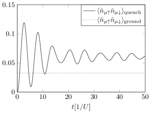
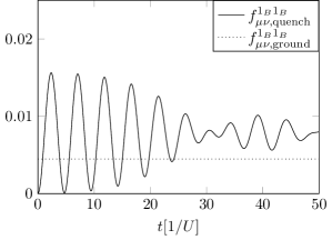
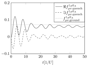
Figure 15: Time-dependence of the quantum depletion, the nearest-neighbour correlation function $f^{1_{B}0_{A}}_{\mu\nu}$, and the next-to-nearest-neighbour correlation function $f^{1_{B}1_{B}}_{\mu\nu}$ in three dimensions after a quench within the Mott phase from $J/U=0$ to $J/U=0.5$ in comparison to their ground state values.

13.3 Quench

Now we consider a quantum quench, i.e., a sudden switch from $J=0$ to some finite value of $J$, where we find the following non-vanishing correlations

$$f^{1_{B}1_{B}}_{\mu\nu,\mathrm{quench}}=-f^{0_{A}0_{A}}_{\mu\nu,\mathrm{quench}} = \frac{1}{N}\sum_{\mathbf{k}}2J^{2}T_{\mathbf{k}}^{2}\,\frac{1-\cos(\omega_{\mathbf{k}}t)}{\omega_{\mathbf{k}}^{2}}\,e^{i(\mathbf{x}_{\mu}-\mathbf{x}_{\nu})\cdot\mathbf{k}}\,,$$ (146)

$$f^{1_{B}0_{A}}_{\mu\nu,\mathrm{quench}}=\left({f}^{0_{A}1_{B}}_{\mu\nu,\mathrm{quench}}\right)^{*} = \frac{1}{N}\sum_{\mathbf{k}}JT_{\mathbf{k}}U\frac{1-\cos(\omega_{\mathbf{k}}t)}{\omega_{\mathbf{k}}^{2}}e^{i(\mathbf{x}_{\mu}-\mathbf{x}_{\nu})\cdot\mathbf{k}}$$ (147)

$$-\frac{i}{N}\sum_{\mathbf{k}}JT_{\mathbf{k}}\,\frac{\sin(\omega_{\mathbf{k}}t)}{\omega_{\mathbf{k}}}\,e^{i(\mathbf{x}_{\mu}-\mathbf{x}_{\nu})\cdot\mathbf{k}}\,.$$

Again, these correlations equilibrate to a quasi-stationary value, which is, however, not thermal. For some of these correlations, this quasi-stationary value lies even below the ground-state correlation, see Fig. 15. The probability to have two or zero particles at a site reads

$$\langle\hat{n}_{\mu s}\hat{n}_{\mu\bar{s}}\rangle_{\mathrm{quench}}=\langle\hat{\bar{n}}_{\mu s}\hat{\bar{n}}_{\mu\bar{s}}\rangle_{\mathrm{quench}}=\frac{1}{N}\sum_{\mathbf{k}}2J^{2}T_{\mathbf{k}}^{2}\,\frac{1-\cos(\omega_{\mathbf{k}}t)}{\omega_{\mathbf{k}}^{2}}\,.$$ (148)

This quantity also equilibrates to a quasi-stationary value of order $1/Z$. In analogy to the bosonic case, this quasi-stationary value could be explained by a small effective temperature – but this small effective temperature then does not work for the other observables, e.g., the correlations.

13.4 Spin modes

So far, we have considered expectations values such as $\langle\hat{c}_{\mu a}^{\dagger}\hat{c}_{\nu b}\hat{n}_{\mu\bar{a}}\hat{n}_{\nu\bar{b}}\rangle$, where – apart from the number operators $\hat{n}_{\mu\bar{a}}$ and $\hat{n}_{\nu\bar{b}}$ – one particle is annihilated at site $\nu$ and one is created at site $\mu$. These operator combinations correspond to a change of the occupation numbers and are thus called charge modes. However, as already indicated in Section 11, there are also other modes which leave the total occupation number of all lattice sites unchanged. Examples are $\langle\hat{c}_{\mu s}^{\dagger}\hat{c}_{\mu\bar{s}}\hat{c}_{\nu\bar{s}}^{\dagger}\hat{c}_{\nu s}\rangle$ or $\langle\hat{n}_{\mu a}\hat{n}_{\nu b}\rangle$ or combinations thereof. Many of these combinations can be expressed in terms of the effective spin operators in (118) via $\langle\hat{S}_{\mu}^{i}\hat{S}_{\nu}^{j}\rangle$. As one would expect from our study of the Bose-Hubbard model, the evolution of these spin modes vanishes to first order in $1/Z$

$$\partial_{t}\langle\hat{S}_{\mu}^{i}\hat{S}_{\nu}^{j}\rangle=\,{\cal O}(1/Z^{2})\,,$$ (149)

consistent with the Heisenberg Hamiltonian (119). In analogy to the $\langle\hat{n}_{\mu}\hat{n}_{\nu}\rangle$-correlator in the bosonic case, one has to go to second order $\,{\cal O}(1/Z^{2})$ in order to calculate these quantities. Fortunately, the charge modes discussed above do not couple to these spin modes to first order in $1/Z$ and hence we can omit them to this level of accuracy.

14 Tilted Fermi-Hubbard Lattice

Motivated by the bosonic case, we now study particle-hole pair creation via tunnelling in a tilted lattice. Again, we assume a spatially constant but possibly time-dependent force on the particles which acts on both spin species in the same way. Accordingly, we modify our Hamiltonian via

$$\hat{H}=-\frac{J}{Z}\sum_{\mu\nu,s}T_{\mu\nu}\hat{c}_{\mu,s}^{\dagger}\hat{c}_{\nu,s}+U\sum_{\mu}\hat{n}_{\mu}^{\uparrow}\hat{n}_{\mu}^{\downarrow}+\sum_{\mu}V_{\mu}(\hat{n}_{\mu}^{\uparrow}+\hat{n}_{\mu}^{\downarrow})\,,$$ (150)

where $V_{\mu}(t)=\mathbf{E}(t)\cdot\mathbf{x}_{\mu}$ denotes the additional potential. Performing the same procedure as before, we find modified equations of motion for the charge modes

$$i\partial_{t}f^{0_{A}0_{A}}_{\mu\nu} = +\frac{J}{Z}\sum_{\kappa\neq\mu,\nu}\left(T_{\mu\kappa}f^{1_{B}0_{A}}_{\kappa\nu}-T_{\kappa\nu}f^{0_{A}1_{B}}_{\mu\kappa}\right)\,,$$ (151)

$$i\partial_{t}f^{0_{A}1_{B}}_{\mu\nu} = +\frac{J}{Z}\sum_{\kappa\neq\mu,\nu}\left(T_{\mu\kappa}f^{1_{B}1_{B}}_{\kappa\nu}-T_{\kappa\nu}f^{0_{A}0_{A}}_{\mu\kappa}\right)$$ (152)

$$+(U+V_{\nu}-V_{\mu})f^{0_{A}1_{B}}_{\mu\nu}-\frac{J}{Z}T_{\mu\nu}\,,$$

$$i\partial_{t}f^{1_{B}0_{A}}_{\mu\nu} = -\frac{J}{Z}\sum_{\kappa\neq\mu,\nu}\left(T_{\kappa\nu}f^{1_{B}1_{B}}_{\mu\kappa}-T_{\mu\kappa}f^{0_{A}0_{A}}_{\kappa\nu}\right)$$ (153)

$$-(U-V_{\nu}+V_{\mu})f^{1_{B}0_{A}}_{\mu\nu}+\frac{J}{Z}T_{\mu\nu}\,,$$

$$i\partial_{t}f^{1_{B}1_{B}}_{\mu\nu} = +\frac{J}{Z}\sum_{\kappa\neq\mu,\nu}\left(T_{\mu\kappa}f^{0_{A}1_{B}}_{\kappa\nu}-T_{\kappa\nu}f^{1_{B}0_{A}}_{\mu\kappa}\right)\,.$$ (154)

In complete analogy to the bosonic case it is possible to factorise the differential equations for the correlation functions. We define effective particle and hole operators such that we have for the correlations functions without source terms

$$\langle\hat{p}_{\mu,A}^{\dagger}\hat{h}_{\nu,B}\rangle = f^{1_{A}0_{B}}_{\mu\nu},\qquad\langle\hat{h}_{\mu,B}^{\dagger}\hat{p}_{\nu,A}\rangle=f^{0_{B}1_{A}}_{\mu\nu},$$ (155)

$$\langle\hat{h}_{\mu,B}^{\dagger}\hat{h}_{\nu,B}\rangle = f^{0_{B}0_{B}}_{\mu\nu},\qquad\langle\hat{p}_{\mu,A}^{\dagger}\hat{p}_{\nu,A}\rangle=f^{1_{A}1_{A}}_{\mu\nu},$$ (156)

$$\langle\hat{h}_{\mu,A}^{\dagger}\hat{h}_{\nu,B}\rangle = f^{0_{A}0_{B}}_{\mu\nu},\qquad\langle\hat{p}_{\mu,B}^{\dagger}\hat{h}_{\nu,B}\rangle=f^{1_{B}0_{B}}_{\mu\nu},$$ (157)

$$\langle\hat{h}_{\mu,B}^{\dagger}\hat{h}_{\nu,A}\rangle = f^{0_{B}0_{A}}_{\mu\nu},\qquad\langle\hat{h}_{\mu,B}^{\dagger}\hat{p}_{\nu,B}\rangle=f^{0_{B}1_{B}}_{\mu\nu},$$ (158)

$$\langle\hat{p}_{\mu,B}^{\dagger}\hat{p}_{\nu,A}\rangle = f^{1_{B}1_{A}}_{\mu\nu},\qquad\langle\hat{h}_{\mu,A}^{\dagger}\hat{p}_{\nu,A}\rangle=f^{0_{A}1_{A}}_{\mu\nu},$$ (159)

$$\langle\hat{p}_{\mu,A}^{\dagger}\hat{p}_{\nu,B}\rangle = f^{1_{A}1_{B}}_{\mu\nu},\qquad\langle\hat{p}_{\mu,A}^{\dagger}\hat{h}_{\nu,A}\rangle=f^{1_{A}0_{A}}_{\mu\nu},$$ (160)

and for the correlation functions with source terms

$$\langle\hat{h}_{\mu,A}^{\dagger}\hat{p}_{\nu,B}\rangle = f^{0_{A}1_{B}}_{\mu\nu},\qquad\langle\hat{h}_{\mu,A}^{\dagger}\hat{h}_{\nu,A}\rangle=f^{0_{A}0_{A}}_{\mu\nu}+\delta_{\mu\nu},$$ (161)

$$\langle\hat{p}_{\mu,B}^{\dagger}\hat{h}_{\nu,A}\rangle = f^{1_{B}0_{A}}_{\mu\nu},\qquad\langle\hat{p}_{\mu,B}^{\dagger}\hat{p}_{\nu,B}\rangle=f^{1_{B}1_{B}}_{\mu\nu}\,.$$ (162)

This allows us to effectively factorise the equations for the correlation functions

$$i\partial_{t}\hat{p}_{\mu,B} = -\frac{J}{Z}\sum_{\kappa\neq\mu}T_{\mu\kappa}\left(\hat{h}_{\kappa,A}+\hat{p}_{\kappa,A}\right)+\left(\frac{U}{2}+V_{\mu}\right)\hat{p}_{\mu,B}$$ (163)

$$i\partial_{t}\hat{h}_{\mu,A} = -\frac{J}{Z}\sum_{\kappa\neq\mu}T_{\mu\kappa}\left(\hat{h}_{\kappa,B}+\hat{p}_{\kappa,B}\right)+\left(-\frac{U}{2}+V_{\mu}\right)\hat{h}_{\mu,A}$$ (164)

$$i\partial_{t}\hat{p}_{\mu,A} = \left(\frac{U}{2}+V_{\mu}\right)\hat{p}_{\mu,A}$$ (165)

$$i\partial_{t}\hat{h}_{\mu,B} = \left(-\frac{U}{2}+V_{\mu}\right)\hat{h}_{\mu,B}\,.$$ (166)

Due to the initial conditions, we can set the operators $\hat{h}_{\mu,B}$ and $\hat{p}_{\mu,A}$ to zero. After Fourier and Peierls transformation (58), we find the symmetric form

$$i\partial_{t}\hat{p}_{\mathbf{k},B} = +\frac{U}{2}\hat{p}_{\mathbf{k},B}-JT_{\mathbf{k}}(t)\hat{h}_{\mathbf{k},A}\,,$$ (167)

$$i\partial_{t}\hat{h}_{\mathbf{k},A} = -\frac{U}{2}\hat{h}_{\mathbf{k},A}-JT_{\mathbf{k}}(t)\hat{p}_{\mathbf{k},B}\,,$$ (168)

where the $T_{\mathbf{k}}(t)$ are time-dependent. Now the line of reasoning is analogous to the Bose-Hubbard model. Initially, the operators evolve according to

$$\hat{h}_{\mathbf{k},A} = e^{+iUt/2}\hat{A}_{\mathbf{k}}\,,$$ (169)

$$\hat{p}_{\mathbf{k},B} = e^{-iUt/2}\hat{B}_{\mathbf{k}}\,,$$ (170)

with $\langle\hat{A}_{\mathbf{k}}^{\dagger}\hat{A}_{\mathbf{p}}\rangle=0$ and $\langle\hat{B}_{\mathbf{k}}^{\dagger}\hat{B}_{\mathbf{p}}\rangle=\delta_{\mathbf{k,p}}$. At the end of the evolution, we find

$$\hat{h}_{\mathbf{k},A} = \left(\alpha_{\mathbf{k}}\hat{A}_{\mathbf{k}}+\beta_{\mathbf{k}}\hat{B}_{\mathbf{k}}\right)e^{+iUt/2}$$ (171)

$$\hat{p}_{\mathbf{k},B} = \left(\beta_{\mathbf{k}}^{*}\hat{A}_{\mathbf{k}}-\alpha_{\mathbf{k}}^{*}\hat{B}_{\mathbf{k}}\right)e^{-iUt/2}\,.$$ (172)

In contrast to the bosonic case (where $|\alpha_{\mathbf{k}}|^{2}-|\beta_{\mathbf{k}}|^{2}=1$), we have $|\alpha_{\mathbf{k}}|^{2}+|\beta_{\mathbf{k}}|^{2}=1$. This difference reflects the fermionic nature of the quasi-particles and will have consequences for the case of resonant hopping (see below). The number of created particle-hole pairs then yields the depletion

$$\langle\hat{n}_{\mu s}\hat{n}_{\mu\bar{s}}\rangle=\langle\hat{\bar{n}}_{\mu s}\hat{\bar{n}}_{\mu\bar{s}}\rangle=\frac{1}{N}\sum_{\mathbf{k}}|\beta_{\mathbf{k}}|^{2}\,.$$ (173)

Note that the equations (167) and (168) are analogous to the Dirac equation in 1+1 dimensions, if we consider a small effective electric field $\mathbf{E}$. In this case, particle-hole pair creation will occur predominantly in the vicinity of those points in $\mathbf{k}$-space, where $T_{\mathbf{k}}$ vanishes, i.e., where the energy gap $\omega_{\mathbf{k}}$ in (138) assumes it minimum. Inserting $\mathbf{k}=\mathbf{k}_{0}+\delta\mathbf{k}$ with $T_{\mathbf{k}_{0}}=0$, we may approximate $T_{\mathbf{k}}(t)$ via

$$T_{\mathbf{k}}(t)\approx[\delta\mathbf{k}+\mathbf{A}(t)]\cdot[\nabla_{\mathbf{k}}T_{\mathbf{k}}]_{\mathbf{k}_{0}}\,.$$ (174)

Inserting this approximation into the equations (167) and (168), we get

$$i\partial_{t}\left(\begin{array}[]{c}\hat{p}_{\mathbf{k},B}\\ \hat{h}_{\mathbf{k},A}\end{array}\right)=\left(\frac{U}{2}\,\sigma^{z}-J[\nabla_{\mathbf{k}}T_{\mathbf{k}}]_{\mathbf{k}_{0}}\cdot[\delta\mathbf{k}+\mathbf{A}(t)]\sigma^{x}\right)\cdot\left(\begin{array}[]{c}\hat{p}_{\mathbf{k},B}\\ \hat{h}_{\mathbf{k},A}\end{array}\right)\,.$$ (179)

This is precisely the same form as a Dirac equation in 1+1 space-time dimensions if we identify the effective speed of light via

$$\mathbf{c}_{\rm eff}=J[\nabla_{\mathbf{k}}T_{\mathbf{k}}]_{\mathbf{k}_{0}}\,,$$ (180)

and the effective mass according to

$$m_{\rm eff}\mathbf{c}_{\rm eff}^{2}=\frac{U}{2}\,.$$ (181)

Note, however, that $\mathbf{c}_{\rm eff}$ depends on $\mathbf{k}_{0}$ in general, i.e., the analogy only works if we single out a specific direction. In contrast to the bosonic case, we do not find a full analogy valid for all $\mathbf{k}$-directions, since the dispersion relation is not isotropic near the minimum in the fermionic case. Nevertheless, we may use the analogy to the 1+1 dimensional Dirac equation in order to estimate the pair creation probability via

$$|\beta_{\mathbf{k}\approx\mathbf{k}_{0}}|^{2}\sim\exp\left\{-\pi\frac{m_{\rm eff}^{2}\mathbf{c}_{\rm eff}^{4}}{\mathbf{c}_{\rm eff}\cdot\mathbf{E}}\right\}=\exp\left\{-\pi\frac{U^{2}}{4J[\nabla_{\mathbf{k}}T_{\mathbf{k}}]_{\mathbf{k}_{0}}\cdot\mathbf{E}}\right\}\,,$$ (182)

where we have assumed a slowly varying field $\mathbf{E}$. This result should be relevant for the investigations of the dielectric break-down in the Fermi-Hubbard model, see, e.g., [100, 101, 102].

15 Resonant Tunnelling

In the previous Section, we have studied the case of small potential gradients, i.e., small effective electric fields $V_{\mu}(t)=\mathbf{E}(t)\cdot\mathbf{x}_{\mu}$, for which we have obtained a quantitative analogy to the Sauter-Schwinger effect, which describes tunnelling from the negative continuum (i.e., the Dirac sea) to the positive continuum. Now let us investigate the case of strong potential gradients. In this case, the lattice structure becomes important and resonance effects play a role. For simplicity, we assume a small hopping rate $J\ll U$ where we can solve the equations for the charge modes (151-154) via time-dependent perturbation theory. In this case, Eq. (152) simplifies to

$$\left(i\partial_{t}-U-V_{\nu}+V_{\mu}\right)f^{0_{A}1_{B}}_{\mu\nu}=-\frac{J}{Z}T_{\mu\nu}+\,{\cal O}(J^{2})\,,$$ (183)

as the other terms $J(T_{\mu\kappa}f^{1_{B}1_{B}}_{\kappa\nu}-T_{\kappa\nu}f^{0_{A}0_{A}}_{\mu\kappa})$ are of higher order in $J$. We see that this equation becomes resonant if $V_{\mu}-V_{\nu}=U$, i.e., if the energy gained by tunnelling from site $\mu$ to site $\nu$ compensates the gap $U+\,{\cal O}(J^{2})$. In this resonance case, the correlation grows linearly with time $f^{0_{A}1_{B}}_{\mu\nu}=iJtT_{\mu\nu}/Z+\,{\cal O}(J^{2})$. Of course, Eq. (153) has the same structure, but becomes resonant for the opposite case $V_{\mu}-V_{\nu}=-U$. Either way, the other two correlators

$$i\partial_{t}f^{0_{A}0_{A}}_{\mu\nu}=\frac{J}{Z}\sum_{\kappa\neq\mu,\nu}\left(T_{\mu\kappa}f^{1_{B}0_{A}}_{\kappa\nu}-T_{\kappa\nu}f^{0_{A}1_{B}}_{\mu\kappa}\right)\,,$$ (184)

and similarly $f^{1_{B}1_{B}}_{\mu\nu}$, grow quadratically $f^{0_{A}0_{A}}_{\mu\nu}\propto J^{2}t^{2}$.

The same perturbative analysis can be done for the bosonic case, if we start from equations (19-21). Alternatively, we could employ the equations (24-26) in Fourier space

$$\left[i\partial_{t}-U+3JT_{\mathbf{k}}(t)\right]f_{\mathbf{k}}^{12} = -\sqrt{2}JT_{\mathbf{k}}(t)(f_{\mathbf{k}}^{11}+f_{\mathbf{k}}^{22}+1)\,,$$

$$\left[i\partial_{t}+U-3JT_{\mathbf{k}}(t)\right]f_{\mathbf{k}}^{21} = +\sqrt{2}JT_{\mathbf{k}}(t)(f_{\mathbf{k}}^{11}+f_{\mathbf{k}}^{22}+1)\,,$$

$$i\partial_{t}f_{\mathbf{k}}^{11}=i\partial_{t}f_{\mathbf{k}}^{22} = \sqrt{2}JT_{\mathbf{k}}(t)(f^{12}_{\mathbf{k}}-f^{21}_{\mathbf{k}})\,,$$

where we have inserted the time-dependent hopping matrix $T_{\mathbf{k}}(t)$ after the Peierls transformation (58). Since $T_{\mathbf{k}}$ is periodic in $\mathbf{k}$ (the $\mathbf{k}$-space is a periodic repetition of the Brillouin zone), the time-dependent hopping matrices $T_{\mathbf{k}}(t)$ are oscillating harmonically for constant potential gradients. Thus the above set of equations corresponds to parametric resonance and can be analysed with Floquet theory. For simplicity, let us assume that the $T_{\mathbf{k}}(t)$ behave after the Peierls transformation as

$$T_{\mathbf{k}}(t)=\frac{1}{Z}\left(e^{iE_{0}t}\chi_{\mathbf{k}}+e^{-iE_{0}t}\chi_{\mathbf{k}}^{*}\right)\,.$$ (185)

In order to solve equations (24-26) we make the Floquet ansatz

$$f^{12}_{\mathbf{k}}=\sum_{n=-\infty}^{\infty}e^{i(\nu+n)E_{0}t}f^{12}_{n}\,,$$ (186)

$$f^{11}_{\mathbf{k}}=f^{22}_{\mathbf{k}}=\sum_{n=-\infty}^{\infty}e^{i(\nu+n)E_{0}t}f^{11}_{n}-\frac{1}{2}\,,$$ (187)

$$f^{21}_{\mathbf{k}}=\sum_{n=-\infty}^{\infty}e^{i(\nu+n)E_{0}t}f^{21}_{n}\,,$$ (188)

where $\nu$ denotes the Floquet exponent and the $f^{ab}_{n}$ are discrete Fourier coefficients of the correlation functions $f_{\mathbf{k}}^{ab}$. In order to satisfy equations (24-26), the functions $f^{ab}_{n}$ have to fulfill the linear system of equations

$$\hat{\mathbf{M}}\cdot\mathbf{f}=\mathbf{0}\,,$$ (189)

where we defined the infinite-dimensional matrix

$$\hat{\mathbf{M}}=\left(\begin{array}[]{ccccccc}....&....&....&&&&\\ &\chi_{\mathbf{k}}\mathbf{M}_{-1}&\mathbf{1}&\chi_{\mathbf{k}}^{*}\mathbf{M}_{-1}&&&\\ &&\chi_{\mathbf{k}}\mathbf{M}_{0}&\mathbf{1}&\chi_{\mathbf{k}}^{*}\mathbf{M}_{0}&&\\ &&&\chi_{\mathbf{k}}\mathbf{M}_{1}&\mathbf{1}&\chi_{\mathbf{k}}^{*}\mathbf{M}_{1}&\\ &&&&....&....&....\end{array}\right)$$ (195)

with

$$\mathbf{M}_{n}=\frac{J}{ZE_{0}}\left(\begin{array}[]{ccc}-\frac{3}{\nu+n+{U}/{E_{0}}}&-\frac{2\sqrt{2}}{\nu+n+{U}/{E_{0}}}&0\\ \frac{2}{\nu+n}&0&-\frac{\sqrt{2}}{\nu+n}\\ 0&\frac{2\sqrt{2}}{\nu+n-{U}/{E_{0}}}&\frac{3}{\nu+n-{U}/{E_{0}}}\end{array}\right)\,,$$ (199)

and the vector

$$\mathbf{f}=(...,f^{12}_{-1},f^{11}_{-1},f^{21}_{-1},f^{12}_{0},f^{11}_{0},f^{21}_{0},f^{12}_{1},f^{11}_{1},f^{21}_{1},...)^{T}\,.$$ (200)

The set of equations (189) has only nontrivial solutions if the determinant of the infinite-dimensional matrix vanishes, that is

$$\Delta(\nu)=\mathrm{Det}(\hat{\mathbf{M}})=0\,.$$ (201)

The above relation determines the Floquet exponent $\nu$ up to multiples of $2\pi$ and it can be shown that $\nu$ satisfies the equality [103]

$$\sin^{2}(\pi\nu)=\sin^{2}\left(\frac{\pi U}{E_{0}}\right)\Delta(0)\,.$$ (202)

If the hopping rate is much smaller than the potential gradient, that is $J\ll E_{0}$, we may expand $\Delta(0)$ in powers of $J/E_{0}$. Using the matrix-identity

$$\mathrm{Det}(\hat{\mathbf{M}})=\exp(\tr\{\ln\hat{\mathbf{M}}\})\,,$$ (203)

we find up to forth order in $J/E_{0}$

$$\sin^{2}\left(\pi\nu\right) = \sin^{2}\left(\frac{\pi U}{E_{0}}\right)\Bigg{[}1+\frac{16J^{2}|\chi_{\mathbf{k}}|^{2}\pi U}{Z^{2}E_{0}(E_{0}^{2}-U^{2})}\cot\left(\frac{\pi U}{E_{0}}\right)$$ (204)

$$+\frac{8J^{4}|\chi_{\mathbf{k}}|^{4}\pi U}{Z^{4}\sin^{2}\left(\frac{\pi U}{E_{0}}\right)}\frac{1}{E_{0}^{2}(E_{0}^{2}-U^{2})^{3}(4E_{0}^{2}-U^{2})}$$

$$\quad\times\Bigg{\{}8\pi U\left(4E_{0}^{4}-5E_{0}^{2}U^{2}+U^{4}\right)\cos\left(\frac{2\pi U}{E_{0}}\right)$$

$$\quad\quad+E_{0}\left(-19E_{0}^{4}+76E_{0}^{2}U^{2}-33U^{4}\right)\sin\left(\frac{2\pi U}{E_{0}}\right)\Bigg{\}}\Bigg{]}\,.$$

Two cases need to be distinguished. In the first case, the right hand side of (204) is between zero and unity, the Floquet exponent is real and the correlation functions are bounded. In the second case, the right hand side of (204) is bigger than unity or smaller than zero, the Floquet exponent acquires an imaginary part and the correlation functions grow exponentially, $f_{\mathbf{k}}^{ab}\sim\exp(\Im\nu tE_{0})$, corresponding to a Floquet resonance.

We find the first resonance being located at $U=E_{0}$ with a width of $\Delta U=2(\Im\nu)_{\mathrm{max}}E_{0}=4\sqrt{2}J|\chi_{\mathbf{k}}|/Z$. The second resonance is located at $U=2E_{0}+16J^{2}|\chi_{\mathbf{k}}|^{2}/(3E_{0}Z^{2})$ and has the width $\Delta U=2(\Im\nu)_{\mathrm{max}}E_{0}=12\sqrt{2}J^{2}|\chi_{\mathbf{k}}|^{2}/(Z^{2}E_{0})$. In principle, there are resonances when $E_{0}/U$ adopts higher integer values but they become smaller for increasing $E_{0}/U$.

In contrast, the correlation functions in the Fermi-Hubbard model do not grow exponentially. This distinction between the bosonic and the fermionic case can already be deduced from the difference of the conserved quantities (28) and (139). While the relation (28) allows in principle arbitrary large values of the correlation functions, we find from (139) that $f_{\mathbf{k}}^{1_{B}1_{B}}$ cannot exceed unity and is therefore bounded.

16 Conclusions & Outlook

For the Bose and the Fermi-Hubbard model, we studied the quantum correlations analytically by using the hierarchy of correlations obtained via a formal expansion into powers of $1/Z$. Starting deep in the Mott regime $J/U\to 0$ with exactly one particle per lattice site, we derived the correlations in the ground state for a finite value of $J$ and after a quantum quench (i.e., suddenly switching on $J$). From these correlations, we can also infer the quantum depletion, i.e., the probability of having zero (“holon”) or two (“doublon”) particles at a given lattice site. It turns out that these observables approach a quasi-equilibrium state some time after the quench – but this quasi-equilibrium state is not thermal. Furthermore, we derived the particle-hole (“doublon-holon”) pair creation probability via tunnelling in tilted lattices and found remarkable analogies to the Sauter-Schwinger effect (i.e., electron-positron pair creation out of the quantum vacuum by an external electric field) in the case of weak tilts. For strong tilts, one obtains resonant tunnelling reminiscent of the Bloch oscillations for non-interacting particles.

For the Bose-Hubbard model, we also studied a quench from the Mott state to the super-fluid regime and calculated the growth of phase coherence. Going up to second order in $1/Z$, we derived the correlations of the number and parity operators, again in the ground state and after a quench. For the Fermi-Hubbard model, we found that the spin and charge modes decouple to first order in $1/Z$. The dynamics of the charge modes (particle-hole excitations) already contributes to first order in $1/Z$ whereas the time-evolution of the spin modes requires going up to the second order in $1/Z$, similar to the number and parity correlations in the bosonic case.

Comparing our analytical results to numerical simulations for bosons on finite-size lattices in one and two spatial dimensions, we found qualitative agreement. Thus, although our analytical approach is formally based on the limit $Z\gg 1$, we expect that our results apply – at least qualitatively – to lattices in three ($Z=6$), two ($Z=4$), or even one ($Z=2$) spatial dimension. There are only a few properties which strongly depend on the dimensionality of the system, one example being the maximum of the parity correlator well within the Mott regime, which occurs in one spatial dimension only. In view of the tremendous experimental progress regarding ultra-cold atoms in optical lattices, for example, most of our predictions should be testable experimentally.

In this paper, we used the zero-temperature Mott phase as our initial state – but the presented method can easily be applied to other initial states. For example, finite initial temperatures can be incorporated as well because our approach is based on density matrices. Even at zero temperature, it should be interesting to study other initial states. In the bosonic case, we could start with $U=0$ (instead of $J=0$), i.e., in the super-fluid phase, where we may use $\rho^{0}_{\mu}=\left|\alpha\right>_{\mu}\!\left<\alpha\right|$ with the coherent state $\hat{b}_{\mu}\left|\alpha\right>_{\mu}=\alpha\left|\alpha\right>_{\mu}$, see, e.g., [41]. In this way, an order parameter $\langle\hat{b}_{\kappa}\rangle\not=0$ is introduced at the expense of making the total particle number ill-defined $[\hat{N},\hat{\rho}_{\mu}]\not=0$. As another possibility, one could assume non-integer filling $\langle\hat{n}_{\mu}\rangle\not\in\mathbb{N}$, where one has a non-vanishing super-fluid component even for arbitrarily small $J$. For example, taking $\langle\hat{n}_{\mu}\rangle<1$, the initial state would be $\rho^{0}_{\mu}=\left|\psi\right>_{\mu}\!\left<\psi\right|$ with $\left|\psi\right>=\alpha\left|0\right>+\beta\left|1\right>$. In these cases, the time-dependence of $\rho^{0}_{\mu}$ will be non-trivial in general. In the fermionic case, an analogous initial state would be $\rho^{0}_{\mu}=\left|\psi\right>_{\mu}\!\left<\psi\right|$ with $\left|\psi\right>=\alpha\left|0^{\uparrow}0^{\downarrow}\right>+\beta\left|1^{\uparrow}1^{\downarrow}\right>$, which could describe a Bose-Einstein condensate of Cooper-like pairs, which may be stabilised by an attractive interaction $U<0$, for example.

17 Appendix: Derivation of the hierarchy

In this Appendix, we derive the hierarchical set of equations for the correlation functions. The quantum evolution of the one-site density matrix can be derived by tracing von Neumann’s equation (6) over all lattice sites but $\mu$ and exploiting the invariance of the trace under cyclic permutations

$$i\partial_{t}\hat{\rho}_{\mu} = \frac{1}{Z}\tr_{\not\mu}\left\{\sum_{\alpha,\beta\neq\mu}\mathcal{L}_{\alpha\beta}\hat{\rho}+\sum_{\alpha\neq\mu}\mathcal{L}^{S}_{\alpha\mu}\hat{\rho}\right\}+\tr_{\not\mu}\left\{\sum_{\alpha\neq\mu}\mathcal{L}_{\alpha}\hat{\rho}+\mathcal{L}_{\mu}\hat{\rho}\right\}$$ (205)

$$= \frac{1}{Z}\sum_{\alpha\neq\mu}\mathcal{L}^{S}_{\mu\alpha}\tr_{\alpha}\{\hat{\rho}_{\mu\kappa}\}+\mathcal{L}_{\mu}\hat{\rho}_{\mu}\,.$$

Using the definition of the two-point correlations given in (3), we arrive at (9). Similarly, the differential equation for the two-particle density matrix can be deduced by tracing over all lattice sites but $\mu$ and $\nu$,

$$i\partial_{t}\hat{\rho}_{\mu\nu} = i\left(\partial_{t}\hat{\rho}_{\mu\nu}^{\mathrm{corr}}+\hat{\rho}_{\mu}\partial_{t}\hat{\rho}_{\nu}+\hat{\rho}_{\nu}\partial_{t}\hat{\rho}_{\mu}\right)$$ (206)

$$= \frac{1}{Z}\sum_{\alpha\neq\mu\nu}\tr_{\alpha}\left\{\mathcal{L}_{\mu\kappa}^{S}\hat{\rho}_{\mu\nu\alpha}\right\}+\frac{1}{Z}\sum_{\alpha\neq\mu\nu}\tr_{\alpha}\left\{\mathcal{L}_{\kappa\nu}^{S}\hat{\rho}_{\mu\nu\alpha}\right\}$$

$$+\frac{1}{Z}\mathcal{L}_{\mu\nu}^{S}\hat{\rho}_{\mu\nu}+\mathcal{L}_{\mu}\hat{\rho}_{\mu\nu}+\mathcal{L}_{\nu}\hat{\rho}_{\mu\nu}\,.$$

With the definitions (3) and the time-evolution for the single-site density matrix (205), we find for the two-point correlation functions (10). The equations (9) and (10) preserve the hierarchy in time if initially $\hat{\rho}_{\mu}=\mathcal{O}(Z^{0})$ and $\hat{\rho}_{\mu\nu}^{\mathrm{corr}}=\mathcal{O}(1/Z)$ holds. In order to derive the full hierarchy, we define the generating functional

$${\cal F}(\hat{\alpha})={\cal F}(\{\hat{\alpha}_{\mu}\})=\ln\left[\tr\left\{\hat{\rho}\bigotimes_{\mu}(\mathbf{1}_{\mu}+\hat{\alpha}_{\mu})\right\}\right]\,,$$ (207)

where $\hat{\rho}$ is the density matrix of the full lattice and

$$\hat{\alpha}_{\mu}=\sum_{m,n}\alpha_{\mu}^{m,n}|m\rangle_{\mu}\langle n|$$ (208)

are arbitrary operators acting on the Hilbert spaces associated to the lattice sites $\mu$ with the local basis $\{\left|n\right>_{\mu}\}$. The role of this functional is to generate all correlated density matrices via the derivatives with respect to these operators $\hat{\alpha}_{\mu}$ which are defined via

$$\frac{\partial{\cal F(\{\alpha\})}}{{\partial\hat{\alpha}_{\mu}}}=\sum_{m,n}|n\rangle_{\mu}\langle m|\,\frac{\partial\cal F(\{\alpha\})}{\partial\alpha^{m,n}_{\mu}}=\sum_{m,n}|n\rangle_{\mu}\langle m|\,\frac{\partial{\cal F}(\{\alpha\})}{\partial\,{{}_{\mu}\!\left<m\right|}\hat{\alpha}_{\mu}\left|n\right>_{\mu}}\,.$$ (209)

If we consider an ensemble ${\cal S}=\{\mu_{1},\dots,\mu_{\ell}\}$ of $\ell$ different lattice sites $\mu_{1}\not=\dots\not=\mu_{\ell}$, we obtain the correlation operators via

$$\hat{\rho}^{\rm corr}_{\cal S}=\left.\frac{\partial}{\partial\hat{\alpha}_{\mu_{1}}}\frac{\partial}{\partial\hat{\alpha}_{\mu_{2}}}\dots\frac{\partial}{\partial\hat{\alpha}_{\mu_{\ell}}}{\cal F}(\hat{\alpha})\right|_{\hat{\alpha}=0}\,.$$ (210)

These operators are related to the corresponding reduced density matrix operator $\rho_{\cal S}$ through the relation

$$\hat{\rho}_{\cal S}=\hat{\rho}_{\mu_{1}\dots\mu_{\ell}}=\sum_{\cup_{i}{\cal P}_{i}={\cal S}}\prod_{i}\hat{\rho}^{\rm corr}_{{\cal P}_{i}}$$ (211)

where the sum runs over all possible segmentations of the subset ${\cal S}$ into partitions ${\cal P}_{i}$ starting from the whole subset ${\cal P}={\cal S}$ and ranging to single lattice sites ${\cal P}_{i}=\{\mu\}$ where $\hat{\rho}^{\rm corr}_{{\cal P}_{i}=\{\mu\}}=\hat{\rho}_{\mu}$ is understood. For two and three lattice sites, the above equation reproduces Eq. (3).

Our derivation is based on the following scaling hierarchy of correlations:

$$\hat{\rho}_{\cal S}^{\rm c}=\,{\cal O}\left(Z^{1-|\cal S|}\right)$$ (212)

where $|\cal S|$ is the number $\ell$ of lattice sites in the set $\cal S$. From the Liouville equation (6), the temporal evolution of ${\cal F}$ is given by

$$i\partial_{t}{\cal F}(\hat{\alpha}) = \sum_{\mu}\tr_{\mu}\left\{\hat{\alpha}_{\mu}\,{\cal L}_{\mu}\frac{\partial{\cal F}}{\partial\hat{\alpha}_{\mu}}\right\}$$

$$+ \frac{1}{Z}\sum_{\mu,\nu}\tr_{\mu\nu}\left\{(\hat{\alpha}_{\mu}+\hat{\alpha}_{\nu}+\hat{\alpha}_{\mu}\hat{\alpha}_{\nu})\,{\cal L}_{\mu\nu}\left(\frac{\partial^{2}{\cal F}}{\partial\hat{\alpha}_{\mu}\partial\hat{\alpha}_{\nu}}+\frac{\partial{\cal F}}{\partial\hat{\alpha}_{\mu}}\frac{\partial{\cal F}}{\partial\hat{\alpha}_{\nu}}\right)\right\}\,.$$

By taking successive derivatives and using the generalised Leibniz rule

$$\frac{\partial}{\partial\hat{\alpha}_{\mu_{1}}}\frac{\partial}{\partial\hat{\alpha}_{\mu_{2}}}\dots\frac{\partial}{\partial\hat{\alpha}_{\mu_{\ell}}}\left[{\cal F}(\hat{\alpha})\right]^{2} = \sum_{{\cal P}\subseteq{\cal S}}^{{\cal P}\cup\bar{\cal P}={\cal S}}\left[\left(\prod_{\mu_{i}\in{\cal P}}\frac{\partial}{\partial\hat{\alpha}_{\mu_{i}}}\right){\cal F}(\hat{\alpha})\right]\times$$ (215)

$$\times\left[\left(\prod_{\mu_{j}\in\bar{\cal P}}\frac{\partial}{\partial\hat{\alpha}_{\mu_{j}}}\right){\cal F}(\hat{\alpha})\right]\,,$$

as well as the the property

$$\frac{\partial^{2}{\cal F}(\hat{\alpha})}{\partial\hat{\alpha}_{\mu}^{2}}=\frac{\partial}{\partial\hat{\alpha}_{\mu}}\frac{\partial}{\partial\hat{\alpha}_{\mu}}{\cal F}(\hat{\alpha})=-\frac{\partial{\cal F}(\hat{\alpha})}{\partial\hat{\alpha}_{\mu}}\frac{\partial{\cal F}(\hat{\alpha})}{\partial\hat{\alpha}_{\mu}}=-\left(\frac{\partial{\cal F}(\hat{\alpha})}{\partial\hat{\alpha}_{\mu}}\right)^{2}\,,$$ (216)

we establish the following set of equations for the correlated density matrices:

$$i\partial_{t}\hat{\rho}^{\rm corr}_{\cal S} = \sum_{\mu\in{\cal S}}\,{\cal L}_{\mu}\hat{\rho}^{\rm corr}_{\cal S}+\frac{1}{Z}\sum_{\mu,\nu\in{\cal S}}\,{\cal L}_{\mu\nu}\,\hat{\rho}^{\rm corr}_{\cal S}$$ (217)

$$+\frac{1}{Z}\sum_{\kappa\notin{\cal S}}\sum_{\mu\in{\cal S}}\tr_{\kappa}\Bigg{[}\,{\cal L}^{S}_{\mu\kappa}\hat{\rho}^{\rm corr}_{{\cal S}\cup{\kappa}}+\sum_{{\cal P}\subseteq{\cal S}\setminus\{\mu\}}^{{\cal P}\cup\bar{\cal P}={\cal S}\setminus\{\mu\}}\,{\cal L}^{S}_{\mu\kappa}\hat{\rho}^{\rm corr}_{\{\mu\}\cup{\cal P}}\,\hat{\rho}^{\rm corr}_{\{\kappa\}\cup\bar{\cal P}}\Bigg{]}$$

$$+\frac{1}{Z}\sum_{\mu,\nu\in{\cal S}}\sum_{{\cal P}\subseteq{\cal S}\setminus\{\mu,\nu\}}^{{\cal P}\cup\bar{\cal P}={\cal S}\setminus\{\mu,\nu\}}\Bigg{\{}\,{\cal L}_{\mu\nu}\,\hat{\rho}^{\rm corr}_{\{\mu\}\cup{\cal P}}\,\hat{\rho}^{\rm corr}_{\{\nu\}\cup\bar{\cal P}}$$

$$-\tr_{\nu}\Bigg{[}\,{\cal L}^{S}_{\mu\nu}(\hat{\rho}^{\rm corr}_{\{\mu,\nu\}\cup\bar{\cal P}}+\sum_{{\cal Q}\subseteq\bar{\cal P}}^{{\cal Q}\cup\bar{\cal Q}=\bar{\cal P}}\hat{\rho}^{\rm corr}_{\{\mu\}\cup{\cal Q}}\,\hat{\rho}^{\rm corr}_{\{\nu\}\cup\bar{\cal Q}})\Bigg{]}\hat{\rho}^{\rm corr}_{\{\nu\}\cup{\cal P}}\Bigg{\}}\,.$$

For $\ell=1$ and $\ell=2$ we recover the equations (9) and (10). A careful inspection of this set of equations shows that the hierarchy in (212) is preserved in time: Imposing the scaling $\hat{\rho}^{\rm corr}_{\cal S}=\,{\cal O}(Z^{1-|\cal S|})$ on the r.h.s. of the above equation, we find that the time derivative on the l.h.s. does also satisfy the hierarchy (212). Therefore, inserting (212) into (217) and taking the limit $Z\rightarrow\infty$, we obtain the leading-order contributions

$$i\partial_{t}\hat{\rho}^{\rm corr}_{\cal S} = \sum_{\mu\in{\cal S}}\,{\cal L}_{\mu}\hat{\rho}^{\rm corr}_{\cal S}+\frac{1}{Z}\sum_{\kappa\notin{\cal S}}\sum_{\mu\in{\cal S}}\tr_{\kappa}\Bigg{[}\sum_{{\cal P}\subseteq{\cal S}\setminus\{\mu\}}^{{\cal P}\cup\bar{\cal P}={\cal S}\setminus\{\mu\}}\,{\cal L}^{S}_{\mu\kappa}\hat{\rho}^{\rm corr}_{\{\mu\}\cup{\cal P}}\,\hat{\rho}^{\rm corr}_{\{\kappa\}\cup\bar{\cal P}}\Bigg{]}$$ (218)

$$+\frac{1}{Z}\sum_{\mu,\nu\in{\cal S}}\sum_{{\cal P}\subseteq{\cal S}\setminus\{\mu,\nu\}}^{{\cal P}\cup\bar{\cal P}={\cal S}\setminus\{\mu,\nu\}}\Bigg{\{}\,{\cal L}_{\mu\nu}\,\hat{\rho}^{\rm corr}_{\{\mu\}\cup{\cal P}}\,\hat{\rho}^{\rm corr}_{\{\nu\}\cup\bar{\cal P}}$$

$$-\tr_{\nu}\Bigg{[}\,{\cal L}^{S}_{\mu\nu}\sum_{{\cal Q}\subseteq\bar{\cal P}}^{{\cal Q}\cup\bar{\cal Q}=\bar{\cal P}}\hat{\rho}^{\rm corr}_{\{\mu\}\cup{\cal Q}}\,\hat{\rho}^{\rm corr}_{\{\nu\}\cup\bar{\cal Q}}\Bigg{]}\hat{\rho}^{\rm corr}_{\{\nu\}\cup{\cal P}}\Bigg{\}}+\,{\cal O}(Z^{-|\cal S|})\,.$$

For $\ell=1$ and $\ell=2$, we recover equations (11) and (12).

In contrast to the exact expression (217), the approximated leading-order equations (218) form a closed set. The exact time evolution (217) of the $|\cal S|$-point correlator $\partial_{t}\hat{\rho}^{\rm corr}_{\cal S}$ also depends on the higher-order correlation term $\hat{\rho}^{\rm corr}_{{\cal S}\cup{\kappa}}$ involving $|{\cal S}|+1$ points. The approximated expression (218), on the other hand, only contains correlators of the same or lower rank. This facilitates the iterative solution of the problem sketched in Section 3. First one solves the zeroth-order equation (11) for $\hat{\rho}_{\mu}^{0}$. Inserting this result $\hat{\rho}_{\mu}^{0}$ into the first-order (in $1/Z$) equation (12) for $\hat{\rho}_{\mu\nu}^{\rm corr}$, we obtain a first-order result for $\hat{\rho}_{\mu\nu}^{\rm corr}$. This first-order result for $\hat{\rho}_{\mu\nu}^{\rm corr}$ can then be inserted into the equation for $\hat{\rho}_{\mu\nu\lambda}^{\rm corr}$ which is of second order $1/Z^{2}$. Furthermore, we may use the first-order result for $\hat{\rho}_{\mu\nu}^{\rm corr}$ in order to obtain a better approximation for the on-site density matrix $\hat{\rho}_{\mu}^{1}$ which is valid to first order in $1/Z$ and contains the quantum depletion etc. Repeating this iteration, we may successively “climb up” to higher and higher orders in $1/Z$.

18 Appendix: Staggered Magnetic Field

We assumed in Section 12 that the initial state of the Fermi-Hubbard system is given by the Néel state. However, for $J=0$ we have infinitely many states with same energy and vanishing total spin. In order to single out the Néel state, we add a staggered magnetic field to the Hubbard Hamiltonian,

$$\hat{H} = -\frac{J}{Z}\sum_{\mu,\nu}T_{\mu\nu}\left(\hat{c}_{\mu\uparrow}^{\dagger}\hat{c}_{\mu\uparrow}+\hat{c}_{\mu\downarrow}^{\dagger}\hat{c}_{\mu\downarrow}\right)$$ (219)

$$+\sum_{\mu}\left(U\hat{n}_{\mu}^{\uparrow}\hat{n}_{\mu}^{\downarrow}-A_{\mu\downarrow}\hat{n}_{\mu}^{\downarrow}-A_{\mu\uparrow}\hat{n}_{\mu}^{\uparrow}\right)\,.$$

If we choose the magnetic field as $A_{\mu\downarrow}(x_{\mu}\in\mathcal{A})=a$, $A_{\mu\downarrow}(x_{\mu}\in\mathcal{B})=0$, $A_{\mu\uparrow}(x_{\mu}\in\mathcal{B})=a$, and $A_{\mu\uparrow}(x_{\mu}\in\mathcal{A})=0$, the Néel state is the unique ground state for $J=0$ at half filling. The Heisenberg equations (121)-(123) read now

$$i\partial_{t}\hat{c}_{\mu s} = -\frac{J}{Z}\sum_{\kappa\neq\mu}T_{\mu\kappa}\hat{c}_{\kappa s}+U\hat{c}_{\mu s}\hat{n}_{\mu\bar{s}}-A_{\mu s}\hat{c}_{\mu s}$$ (220)

$$i\partial_{t}\hat{c}_{\mu s}^{\dagger} = \frac{J}{Z}\sum_{\kappa\neq\mu}T_{\mu\kappa}\hat{c}^{\dagger}_{\kappa s}-U\hat{c}^{\dagger}_{\mu s}\hat{n}_{\mu\bar{s}}+A_{\mu s}\hat{c}^{\dagger}_{\mu s}$$ (221)

$$i\partial_{t}\hat{n}_{\mu s} = -i\partial_{t}\hat{\bar{n}}_{\mu s}=\frac{J}{Z}\sum_{\kappa\neq\mu}T_{\mu\kappa}\left(\hat{c}_{\kappa s}^{\dagger}\hat{c}_{\mu s}-\hat{c}_{\mu s}^{\dagger}\hat{c}_{\kappa s}\right)\,,$$ (222)

To first order in $1/Z$, we find the closed set of differential equations, cf. Eqs. (124)-(127),

$$i\partial_{t}\langle\hat{c}_{\mu a}^{\dagger}\hat{c}_{\nu b}\hat{n}_{\mu\bar{a}}\hat{n}_{\nu\bar{b}}\rangle = \frac{J}{Z}\sum_{\kappa\neq\mu,\nu}T_{\mu\kappa}\langle\hat{c}_{\kappa a}^{\dagger}\hat{c}_{\nu b}(\hat{n}_{\kappa\bar{a}}+\hat{\bar{n}}_{\kappa\bar{a}})\hat{n}_{\nu\bar{b}}\rangle\langle\hat{n}_{\mu\bar{a}}\rangle_{0}$$ (223)

$$-\frac{J}{Z}\sum_{\kappa\neq\mu,\nu}T_{\nu\kappa}\langle\hat{c}_{\mu a}^{\dagger}\hat{c}_{\kappa b}\hat{n}_{\mu\bar{a}}(\hat{n}_{\kappa\bar{b}}+\hat{\bar{n}}_{\kappa\bar{b}})\rangle\langle\hat{n}_{\nu\bar{b}}\rangle_{0}$$

$$+(A_{\mu a}-A_{\nu b})\langle\hat{c}_{\mu a}^{\dagger}\hat{c}_{\nu b}\hat{n}_{\mu\bar{a}}\hat{n}_{\nu\bar{b}}\rangle$$

$$+\frac{J}{Z}T_{\mu\nu}\langle\hat{c}_{\nu a}^{\dagger}\hat{c}_{\nu b}\hat{n}_{\mu\bar{a}}\hat{n}_{\nu\bar{b}}\rangle_{0}-\frac{J}{Z}T_{\mu\nu}\langle\hat{c}_{\mu a}^{\dagger}\hat{c}_{\mu b}\hat{n}_{\mu\bar{a}}\hat{n}_{\nu\bar{b}}\rangle_{0}$$

$$i\partial_{t}\langle\hat{c}_{\mu a}^{\dagger}\hat{c}_{\nu b}\hat{n}_{\mu\bar{a}}\hat{\bar{n}}_{\nu\bar{b}}\rangle = \frac{J}{Z}\sum_{\kappa\neq\mu,\nu}T_{\mu\kappa}\langle\hat{c}_{\kappa a}^{\dagger}\hat{c}_{\nu b}(\hat{n}_{\kappa\bar{a}}+\hat{\bar{n}}_{\kappa\bar{a}})\hat{\bar{n}}_{\nu\bar{b}}\rangle\langle\hat{n}_{\mu\bar{a}}\rangle_{0}$$ (224)

$$-\frac{J}{Z}\sum_{\kappa\neq\mu,\nu}T_{\nu\kappa}\langle\hat{c}_{\mu a}^{\dagger}\hat{c}_{\kappa b}\hat{n}_{\mu\bar{a}}(\hat{n}_{\kappa\bar{b}}+\hat{\bar{n}}_{\kappa\bar{b}})\rangle\langle\hat{\bar{n}}_{\nu\bar{b}}\rangle_{0}$$

$$-(U-A_{\mu a}+A_{\nu b})\langle\hat{c}_{\mu a}^{\dagger}\hat{c}_{\nu b}\hat{n}_{\mu\bar{a}}\hat{\bar{n}}_{\nu\bar{b}}\rangle$$

$$+\frac{J}{Z}T_{\mu\nu}\langle\hat{c}_{\nu a}^{\dagger}\hat{c}_{\nu b}\hat{n}_{\mu\bar{a}}\hat{\bar{n}}_{\nu\bar{b}}\rangle_{0}-\frac{J}{Z}T_{\mu\nu}\langle\hat{c}_{\mu a}^{\dagger}\hat{c}_{\mu b}\hat{n}_{\mu\bar{a}}\hat{\bar{n}}_{\nu\bar{b}}\rangle_{0}$$

$$i\partial_{t}\langle\hat{c}_{\mu a}^{\dagger}\hat{c}_{\nu b}\hat{\bar{n}}_{\mu\bar{a}}\hat{n}_{\nu\bar{b}}\rangle = \frac{J}{Z}\sum_{\kappa\neq\mu,\nu}T_{\mu\kappa}\langle\hat{c}_{\kappa a}^{\dagger}\hat{c}_{\nu b}(\hat{n}_{\kappa\bar{a}}+\hat{\bar{n}}_{\kappa\bar{a}})\hat{n}_{\nu\bar{b}}\rangle\langle\hat{\bar{n}}_{\mu\bar{a}}\rangle_{0}$$ (225)

$$-\frac{J}{Z}\sum_{\kappa\neq\mu,\nu}T_{\nu\kappa}\langle\hat{c}_{\mu a}^{\dagger}\hat{c}_{\kappa b}\hat{\bar{n}}_{\mu\bar{a}}(\hat{n}_{\kappa\bar{b}}+\hat{\bar{n}}_{\kappa\bar{b}})\rangle\langle\hat{n}_{\nu\bar{b}}\rangle_{0}$$

$$+(U+A_{\mu a}-A_{\nu b})\langle\hat{c}_{\mu a}^{\dagger}\hat{c}_{\nu b}\hat{\bar{n}}_{\mu\bar{a}}\hat{n}_{\nu\bar{b}}\rangle$$

$$+\frac{J}{Z}T_{\mu\nu}\langle\hat{c}_{\nu a}^{\dagger}\hat{c}_{\nu b}\hat{\bar{n}}_{\mu\bar{a}}\hat{n}_{\nu\bar{b}}\rangle_{0}-\frac{J}{Z}T_{\mu\nu}\langle\hat{c}_{\mu a}^{\dagger}\hat{c}_{\mu b}\hat{\bar{n}}_{\mu\bar{a}}\hat{n}_{\nu\bar{b}}\rangle_{0}$$

$$i\partial_{t}\langle\hat{c}_{\mu a}^{\dagger}\hat{c}_{\nu b}\hat{\bar{n}}_{\mu\bar{a}}\hat{\bar{n}}_{\nu\bar{b}}\rangle = \frac{J}{Z}\sum_{\kappa\neq\mu,\nu}T_{\mu\kappa}\langle\hat{c}_{\kappa a}^{\dagger}\hat{c}_{\nu b}(\hat{n}_{\kappa\bar{a}}+\hat{\bar{n}}_{\kappa\bar{a}})\hat{\bar{n}}_{\nu\bar{b}}\rangle\langle\hat{\bar{n}}_{\mu\bar{a}}\rangle_{0}$$ (226)

$$-\frac{J}{Z}\sum_{\kappa\neq\mu,\nu}T_{\nu\kappa}\langle\hat{c}_{\mu a}^{\dagger}\hat{c}_{\kappa b}\hat{\bar{n}}_{\mu\bar{a}}(\hat{n}_{\kappa\bar{b}}+\hat{\bar{n}}_{\kappa\bar{b}})\rangle\langle\hat{\bar{n}}_{\nu\bar{b}}\rangle_{0}$$

$$+(A_{\mu a}-A_{\nu b})\langle\hat{c}_{\mu a}^{\dagger}\hat{c}_{\nu b}\hat{\bar{n}}_{\mu\bar{a}}\hat{\bar{n}}_{\nu\bar{b}}\rangle$$

$$+\frac{J}{Z}T_{\mu\nu}\langle\hat{c}_{\nu a}^{\dagger}\hat{c}_{\nu b}\hat{\bar{n}}_{\mu\bar{a}}\hat{\bar{n}}_{\nu\bar{b}}\rangle_{0}-\frac{J}{Z}T_{\mu\nu}\langle\hat{c}_{\mu a}^{\dagger}\hat{c}_{\mu b}\hat{\bar{n}}_{\mu\bar{a}}\hat{\bar{n}}_{\nu\bar{b}}\rangle_{0}\,.$$

If $x_{\mu}\in A$ and $x_{\nu}\in B$ we denote the correlations $\langle\hat{c}_{\mu\downarrow}^{\dagger}\hat{c}_{\mu\downarrow}\hat{n}_{\mu\uparrow}\hat{n}_{\nu\uparrow}\rangle=f_{\mu\nu}^{1_{A}1_{B}}$, $\langle\hat{c}_{\mu\downarrow}^{\dagger}\hat{c}_{\mu\downarrow}\hat{\bar{n}}_{\mu\uparrow}\hat{n}_{\nu\uparrow}\rangle=f_{\mu\nu}^{0_{A}1_{B}}$, etc. Inserting the zeroth-order Néel state, we find four equations which fully decouple, cf. Eq. (128),

$$i\partial_{t}f^{1_{A}0_{B}}_{\mu\nu} = -(U-a)f^{1_{A}0_{B}}_{\mu\nu}$$ (227)

$$i\partial_{t}f^{0_{B}1_{A}}_{\mu\nu} = (U-a)f^{0_{B}1_{A}}_{\mu\nu}$$ (228)

$$i\partial_{t}f^{0_{B}0_{B}}_{\mu\nu} = 0$$ (229)

$$i\partial_{t}f^{1_{A}1_{A}}_{\mu\nu} = 0\,.$$ (230)

In general, these four correlations are sources in the following four pairs of coupled equations, cf. Eqs. (129)-(132),

$$i\partial_{t}f^{0_{A}0_{B}}_{\mu\nu} = \frac{J}{Z}\sum_{\kappa\neq{\mu,\nu}}T_{\mu\kappa}\left(f^{1_{B}0_{B}}_{\kappa\nu}+f^{0_{B}0_{B}}_{\kappa\nu}\right)+af^{0_{A}0_{B}}_{\mu\nu}$$ (231)

$$i\partial_{t}f^{1_{B}0_{B}}_{\mu\nu} = \frac{J}{Z}\sum_{\kappa\neq{\mu,\nu}}T_{\mu\kappa}\left(f^{0_{A}0_{B}}_{\kappa\nu}+f^{1_{A}0_{B}}_{\kappa\nu}\right)-Uf^{1_{B}0_{B}}_{\mu\nu}\,,$$ (232)

$$i\partial_{t}f^{0_{B}0_{A}}_{\mu\nu} = -\frac{J}{Z}\sum_{\kappa\neq{\mu,\nu}}T_{\kappa\nu}\left(f^{0_{B}1_{B}}_{\mu\kappa}+f^{0_{B}0_{B}}_{\mu\kappa}\right)-af^{0_{B}0_{A}}_{\mu\nu}$$ (233)

$$i\partial_{t}f^{0_{B}1_{B}}_{\mu\nu} = -\frac{J}{Z}\sum_{\kappa\neq{\mu,\nu}}T_{\kappa\nu}\left(f^{0_{B}0_{A}}_{\mu\kappa}+f^{0_{B}1_{A}}_{\mu\kappa}\right)+Uf^{0_{B}1_{B}}_{\mu\nu}\,,$$ (234)

$$i\partial_{t}f^{1_{B}1_{A}}_{\mu\nu} = \frac{J}{Z}\sum_{\kappa\neq{\mu,\nu}}T_{\mu\kappa}\left(f^{0_{A}1_{A}}_{\kappa\nu}+f^{1_{A}1_{A}}_{\kappa\nu}\right)-af^{1_{B}1_{A}}_{\mu\nu}$$ (235)

$$i\partial_{t}f^{0_{A}1_{A}}_{\mu\nu} = \frac{J}{Z}\sum_{\kappa\neq{\mu,\nu}}T_{\mu\kappa}\left(f^{0_{B}1_{A}}_{\kappa\nu}+f^{1_{B}1_{A}}_{\kappa\nu}\right)+Uf^{0_{A}1_{A}}_{\mu\nu}\,,$$ (236)

$$i\partial_{t}f^{1_{A}1_{B}}_{\mu\nu} = -\frac{J}{Z}\sum_{\kappa\neq{\mu,\nu}}T_{\kappa\nu}\left(f^{1_{A}0_{A}}_{\mu\kappa}+f^{1_{A}1_{A}}_{\mu\kappa}\right)+af^{1_{A}1_{B}}_{\mu\nu}$$ (237)

$$i\partial_{t}f^{1_{A}0_{A}}_{\mu\nu} = -\frac{J}{Z}\sum_{\kappa\neq{\mu,\nu}}T_{\kappa\nu}\left(f^{1_{A}0_{B}}_{\mu\kappa}+f^{1_{A}1_{B}}_{\mu\kappa}\right)-Uf^{1_{A}0_{A}}_{\mu\nu}\,.$$ (238)

The eigenfrequencies of these equations read now

$$\omega_{\mathbf{k}}^{\pm}=\frac{U+a\pm\sqrt{4J^{2}T_{\mathbf{k}}^{2}+(U-a)^{2}}}{2}\,.$$ (239)

In contrast to the eigenmodes (133) we see that the modes (239) have a gap in the limit $J\rightarrow 0$. This enables us to switch on $J$ and then switch off $a$ adiabatically in order to have a well-defined initial state without correlations. Furthermore we have the four coupled equations, cf. Eqs. (134)-(137),

$$i\partial_{t}f^{0_{A}0_{A}}_{\mu\nu} = \frac{J}{Z}\sum_{\kappa\neq{\mu,\nu}}\left\{T_{\mu\kappa}\left(f^{0_{B}0_{A}}_{\kappa\nu}+f^{1_{B}0_{A}}_{\kappa\nu}\right)-T_{\kappa\nu}\left(f^{0_{A}0_{B}}_{\mu\kappa}+f^{0_{A}1_{B}}_{\mu\kappa}\right)\right\}$$ (240)

$$i\partial_{t}f^{0_{A}1_{B}}_{\mu\nu} = \frac{J}{Z}\sum_{\kappa\neq{\mu,\nu}}\left\{T_{\mu\kappa}\left(f^{1_{B}1_{B}}_{\kappa\nu}+f^{0_{B}1_{B}}_{\kappa\nu}\right)-T_{\kappa\nu}\left(f^{0_{A}0_{A}}_{\mu\kappa}+f^{0_{A}1_{A}}_{\mu\kappa}\right)\right\}$$ (241)

$$+(U+a)f^{0_{A}1_{B}}_{\mu\nu}-\frac{J}{Z}T_{\mu\nu}$$

$$i\partial_{t}f^{1_{B}0_{A}}_{\mu\nu} = \frac{J}{Z}\sum_{\kappa\neq{\mu,\nu}}\left\{T_{\mu\kappa}\left(f^{0_{A}0_{A}}_{\kappa\nu}+f^{1_{A}0_{A}}_{\kappa\nu}\right)-T_{\kappa\nu}\left(f^{1_{B}1_{B}}_{\mu\kappa}+f^{1_{B}0_{B}}_{\mu\kappa}\right)\right\}$$ (242)

$$-(U+a)f^{1_{B}0_{A}}_{\mu\nu}+\frac{J}{Z}T_{\mu\nu}$$

$$i\partial_{t}f^{1_{B}1_{B}}_{\mu\nu} = \frac{J}{Z}\sum_{\kappa\neq{\mu,\nu}}\left\{T_{\mu\kappa}\left(f^{0_{A}1_{B}}_{\kappa\nu}+f^{1_{A}1_{B}}_{\kappa\nu}\right)-T_{\kappa\nu}\left(f^{1_{B}0_{A}}_{\mu\kappa}+f^{1_{B}1_{A}}_{\mu\kappa}\right)\right\}\,.$$ (243)

The eigenfrequencies of these equations read now

$$\omega_{\mathbf{k}}^{\pm}=\pm\sqrt{4J^{2}T_{\mathbf{k}}^{2}+(U+a)^{2}}\,.$$ (244)

19 Appendix: Second-order Equations

The differential equation for the three-point correlator reads

$$i\partial_{t}\hat{\rho}_{\alpha\beta\gamma}^{\mathrm{corr}} = \hat{\mathcal{L}}_{\alpha}\hat{\rho}_{\alpha\beta\gamma}^{\mathrm{corr}}+\frac{1}{Z}\hat{\mathcal{L}}^{S}_{\alpha\beta}\left(\hat{\rho}_{\alpha}\hat{\rho}^{\mathrm{corr}}_{\beta\gamma}+\hat{\rho}_{\beta}\hat{\rho}^{\mathrm{corr}}_{\alpha\gamma}\right)$$ (245)

$$+\frac{1}{Z}\sum_{\kappa\neq\{\alpha,\beta,\gamma\}}\mathrm{tr}_{\kappa}\left\{\hat{\mathcal{L}}^{S}_{\alpha\kappa}\left(\hat{\rho}^{\mathrm{corr}}_{\alpha\beta\gamma}\hat{\rho}_{\kappa}+\hat{\rho}^{\mathrm{corr}}_{\alpha\beta}\hat{\rho}^{\mathrm{corr}}_{\kappa\gamma}+\hat{\rho}^{\mathrm{corr}}_{\alpha\gamma}\hat{\rho}^{\mathrm{corr}}_{\kappa\beta}+\hat{\rho}_{\alpha}\hat{\rho}^{\mathrm{corr}}_{\kappa\beta\gamma}\right)\right\}$$

$$-\frac{1}{Z}\hat{\rho}_{\alpha\gamma}^{\mathrm{corr}}\mathrm{tr}_{\alpha}\left\{\hat{\mathcal{L}}^{S}_{\alpha\beta}\hat{\rho}_{\beta}\hat{\rho}_{\alpha}\right\}-\frac{1}{Z}\hat{\rho}_{\alpha\beta}^{\mathrm{corr}}\mathrm{tr}_{\alpha}\left\{\hat{\mathcal{L}}^{S}_{\alpha\gamma}\hat{\rho}_{\gamma}\hat{\rho}_{\alpha}\right\}$$

$$-\frac{1}{Z}\hat{\rho}_{\alpha}\mathrm{tr}_{\alpha}\left\{\hat{\mathcal{L}}_{\alpha\beta}^{S}\hat{\rho}_{\beta\gamma}^{\mathrm{corr}}\hat{\rho}_{\alpha}+\hat{\mathcal{L}}_{\alpha\beta}^{S}\hat{\rho}_{\beta}\hat{\rho}_{\alpha\gamma}^{\mathrm{corr}}\right\}$$

$$-\frac{1}{Z}\hat{\rho}_{\alpha}\mathrm{tr}_{\alpha}\left\{\hat{\mathcal{L}}_{\alpha\gamma}^{S}\hat{\rho}_{\gamma\beta}^{\mathrm{corr}}\hat{\rho}_{\alpha}+\hat{\mathcal{L}}_{\alpha\gamma}^{S}\hat{\rho}_{\gamma}\hat{\rho}_{\alpha\beta}^{\mathrm{corr}}\right\}$$

$$+(\alpha\rightarrow\beta,\beta\rightarrow\gamma,\gamma\rightarrow\alpha)+(\alpha\rightarrow\gamma,\gamma\rightarrow\beta,\beta\rightarrow\alpha)$$

$$+\mathcal{O}(1/Z^{3})\,.$$

In the following we use the matrix elements of $\hat{\rho}_{\mu\nu}^{\mathrm{corr}}$ and $\hat{\rho}_{\mu}$ in order $1/Z$ and define

$$\hat{\rho}_{\alpha\beta\gamma}^{\mathrm{corr}}=\sum_{a,a^{\prime},b,b^{\prime},c,c^{\prime}}\rho_{\alpha\beta\gamma}^{aa^{\prime}bb^{\prime}cc^{\prime}}|a\rangle_{\alpha}\langle a^{\prime}|\otimes|b\rangle_{\beta}\langle b^{\prime}|\otimes|c\rangle_{\gamma}\langle c^{\prime}|\,.$$ (246)

All three-point correlations can be deduced by permutation and complex conjugation from the following set of differential equations

$$i\partial_{t}\rho_{\alpha\beta\gamma}^{001001} = \frac{J}{Z}\sum_{\kappa\neq\alpha,\beta,\gamma}T_{\beta\kappa}\left(\rho_{\alpha\kappa\gamma}^{001001}+\sqrt{2}\rho_{\alpha\kappa\gamma}^{002101}\right)$$ (247)

$$-\frac{J}{Z}\sum_{\kappa\neq\alpha,\beta,\gamma}T_{\gamma\kappa}\left(\rho_{\alpha\beta\kappa}^{001001}+\sqrt{2}\rho_{\alpha\beta\kappa}^{001012}\right)$$

$$+\frac{J}{Z}\sum_{\kappa\neq\alpha,\beta,\gamma}T_{\alpha\kappa}f^{11}_{\alpha\beta}\left(f^{11}_{\kappa\gamma}+\sqrt{2}f^{12}_{\kappa\gamma}\right)$$

$$-\frac{J}{Z}\sum_{\kappa\neq\alpha,\beta,\gamma}T_{\alpha\kappa}f^{11}_{\alpha\gamma}\left(f^{11}_{\kappa\beta}+\sqrt{2}f^{21}_{\kappa\beta}\right)$$

$$i\partial_{t}\rho_{\alpha\beta\gamma}^{001012} = -U\rho_{\alpha\beta\gamma}^{001012}+\frac{J}{Z}\sum_{\kappa\neq\alpha,\beta,\gamma}T_{\beta\kappa}\left(\rho_{\alpha\kappa\gamma}^{001012}+\sqrt{2}\rho_{\alpha\kappa\gamma}^{002112}\right)$$ (248)

$$+\frac{J}{Z}\sum_{\kappa\neq\alpha,\beta,\gamma}T_{\gamma\kappa}\left(\sqrt{2}\rho_{\alpha\beta\kappa}^{001001}+2\rho_{\alpha\beta\kappa}^{001012}\right)$$

$$+\frac{J}{Z}\sum_{\kappa\neq\alpha,\beta,\gamma}T_{\alpha\kappa}f^{11}_{\alpha\beta}\left(f^{21}_{\kappa\gamma}+\sqrt{2}f^{22}_{\kappa\gamma}\right)$$

$$-\frac{J}{Z}\sum_{\kappa\neq\alpha,\beta,\gamma}T_{\alpha\kappa}f^{21}_{\alpha\gamma}\left(f^{11}_{\kappa\beta}+\sqrt{2}f^{21}_{\kappa\beta}\right)+\frac{J}{Z}T_{\alpha\gamma}\sqrt{2}f^{11}_{\alpha\beta}$$

$$i\partial_{t}\rho_{\alpha\beta\gamma}^{002101} = U\rho_{\alpha\beta\gamma}^{002101}-\frac{J}{Z}\sum_{\kappa\neq\alpha,\beta,\gamma}T_{\beta\kappa}\left(\sqrt{2}\rho_{\alpha\kappa\gamma}^{001001}+2\rho_{\alpha\kappa\gamma}^{002101}\right)$$ (249)

$$-\frac{J}{Z}\sum_{\kappa\neq\alpha,\beta,\gamma}T_{\gamma\kappa}\left(\rho_{\alpha\beta\kappa}^{002101}+\sqrt{2}\rho_{\alpha\beta\kappa}^{002112}\right)$$

$$+\frac{J}{Z}\sum_{\kappa\neq\alpha,\beta,\gamma}T_{\alpha\kappa}f^{12}_{\alpha\beta}\left(f^{11}_{\kappa\gamma}+\sqrt{2}f^{12}_{\kappa\gamma}\right)$$

$$-\frac{J}{Z}\sum_{\kappa\neq\alpha,\beta,\gamma}T_{\alpha\kappa}f^{11}_{\alpha\gamma}\left(f^{12}_{\kappa\beta}+\sqrt{2}f^{22}_{\kappa\beta}\right)-\frac{J}{Z}T_{\alpha\beta}\sqrt{2}f^{11}_{\alpha\gamma}$$

$$i\partial_{t}\rho_{\alpha\beta\gamma}^{002112} = -\frac{J}{Z}\sum_{\kappa\neq\alpha,\beta,\gamma}T_{\beta\kappa}\left(\sqrt{2}\rho_{\alpha\kappa\gamma}^{001012}+2\rho_{\alpha\kappa\gamma}^{002112}\right)$$ (250)

$$+\frac{J}{Z}\sum_{\kappa\neq\alpha,\beta,\gamma}T_{\gamma\kappa}\left(\sqrt{2}\rho_{\alpha\beta\kappa}^{002101}+2\rho_{\alpha\beta\kappa}^{002112}\right)$$

$$+\frac{J}{Z}\sum_{\kappa\neq\alpha,\beta,\gamma}T_{\alpha\kappa}f^{12}_{\alpha\beta}\left(f^{21}_{\kappa\gamma}+\sqrt{2}f^{22}_{\kappa\gamma}\right)$$

$$-\frac{J}{Z}\sum_{\kappa\neq\alpha,\beta,\gamma}T_{\alpha\kappa}f^{21}_{\alpha\gamma}\left(f^{12}_{\kappa\beta}+\sqrt{2}f^{22}_{\kappa\beta}\right)$$

$$-\frac{J}{Z}T_{\alpha\beta}\sqrt{2}f^{21}_{\alpha\gamma}+\frac{J}{Z}T_{\alpha\gamma}\sqrt{2}f^{12}_{\alpha\beta}$$

$$i\partial_{t}\rho_{\alpha\beta\gamma}^{221001} = \frac{J}{Z}\sum_{\kappa\neq\alpha,\beta,\gamma}T_{\beta\kappa}\left(\rho_{\alpha\kappa\gamma}^{221001}+\sqrt{2}\rho_{\alpha\kappa\gamma}^{222101}\right)$$ (251)

$$-\frac{J}{Z}\sum_{\kappa\neq\alpha,\beta,\gamma}T_{\gamma\kappa}\left(\rho_{\alpha\beta\kappa}^{221001}+\sqrt{2}\rho_{\alpha\beta\kappa}^{221012}\right)$$

$$-\frac{J}{Z}\sum_{\kappa\neq\alpha,\beta,\gamma}T_{\alpha\kappa}f^{21}_{\alpha\beta}\left(f^{11}_{\kappa\gamma}+\sqrt{2}f^{12}_{\kappa\gamma}\right)$$

$$+\frac{J}{Z}\sum_{\kappa\neq\alpha,\beta,\gamma}T_{\alpha\kappa}\sqrt{2}f^{12}_{\alpha\gamma}\left(f^{11}_{\kappa\beta}+\sqrt{2}f^{21}_{\kappa\beta}\right)$$

$$-\frac{J}{Z}T_{\alpha\gamma}\sqrt{2}f^{21}_{\alpha\beta}+\frac{J}{Z}T_{\alpha\beta}\sqrt{2}f^{12}_{\alpha\gamma}$$

$$i\partial_{t}\rho_{\alpha\beta\gamma}^{221012} = -U\rho_{\alpha\beta\gamma}^{221012}+\frac{J}{Z}\sum_{\kappa\neq\alpha,\beta,\gamma}T_{\beta\kappa}\left(\rho_{\alpha\kappa\gamma}^{221012}+\sqrt{2}\rho_{\alpha\kappa\gamma}^{222112}\right)$$ (252)

$$+\frac{J}{Z}\sum_{\kappa\neq\alpha,\beta,\gamma}T_{\gamma\kappa}\left(\sqrt{2}\rho_{\alpha\beta\kappa}^{221001}+2\rho_{\alpha\beta\kappa}^{221012}\right)$$

$$-\frac{J}{Z}\sum_{\kappa\neq\alpha,\beta,\gamma}T_{\alpha\kappa}\sqrt{2}f^{21}_{\alpha\beta}\left(f^{21}_{\kappa\gamma}+\sqrt{2}f^{22}_{\kappa\gamma}\right)$$

$$+\frac{J}{Z}\sum_{\kappa\neq\alpha,\beta,\gamma}T_{\alpha\kappa}\sqrt{2}f^{22}_{\alpha\gamma}\left(f^{11}_{\kappa\beta}+\sqrt{2}f^{21}_{\kappa\beta}\right)+\frac{J}{Z}T_{\alpha\beta}\sqrt{2}f^{22}_{\alpha\gamma}$$

$$i\partial_{t}\rho_{\alpha\beta\gamma}^{222101} = U\rho_{\alpha\beta\gamma}^{222101}-\frac{J}{Z}\sum_{\kappa\neq\alpha,\beta,\gamma}T_{\beta\kappa}\left(\sqrt{2}\rho_{\alpha\kappa\gamma}^{221001}+2\rho_{\alpha\kappa\gamma}^{222101}\right)$$ (253)

$$-\frac{J}{Z}\sum_{\kappa\neq\alpha,\beta,\gamma}T_{\gamma\kappa}\left(\rho_{\alpha\beta\kappa}^{222101}+\sqrt{2}\rho_{\alpha\beta\kappa}^{222112}\right)$$

$$-\frac{J}{Z}\sum_{\kappa\neq\alpha,\beta,\gamma}T_{\alpha\kappa}\sqrt{2}f^{22}_{\alpha\beta}\left(f^{11}_{\kappa\gamma}+\sqrt{2}f^{12}_{\kappa\gamma}\right)$$

$$+\frac{J}{Z}\sum_{\kappa\neq\alpha,\beta,\gamma}T_{\alpha\kappa}\sqrt{2}f^{12}_{\alpha\gamma}\left(f^{12}_{\kappa\beta}+\sqrt{2}f^{22}_{\kappa\beta}\right)-\frac{J}{Z}T_{\alpha\gamma}\sqrt{2}f^{22}_{\alpha\beta}$$

$$i\partial_{t}\rho_{\alpha\beta\gamma}^{222112} = -\frac{J}{Z}\sum_{\kappa\neq\alpha,\beta,\gamma}T_{\beta\kappa}\left(\sqrt{2}\rho_{\alpha\kappa\gamma}^{221012}+2\rho_{\alpha\kappa\gamma}^{222112}\right)$$

$$+\frac{J}{Z}\sum_{\kappa\neq\alpha,\beta,\gamma}T_{\gamma\kappa}\left(\sqrt{2}\rho_{\alpha\beta\kappa}^{222101}+2\rho_{\alpha\beta\kappa}^{222112}\right)$$

$$-\frac{J}{Z}\sum_{\kappa\neq\alpha,\beta,\gamma}T_{\alpha\kappa}\sqrt{2}f^{22}_{\alpha\beta}\left(f^{21}_{\kappa\gamma}+\sqrt{2}f^{22}_{\kappa\gamma}\right)$$

$$+\frac{J}{Z}\sum_{\kappa\neq\alpha,\beta,\gamma}T_{\alpha\kappa}\sqrt{2}f^{22}_{\alpha\gamma}\left(f^{12}_{\kappa\beta}+\sqrt{2}f^{22}_{\kappa\beta}\right)$$

$$i\partial_{t}\rho_{\alpha\beta\gamma}^{111001} = \frac{J}{Z}\sum_{\kappa\neq\alpha,\beta,\gamma}T_{\beta\kappa}\left(\rho_{\alpha\kappa\gamma}^{111001}+\sqrt{2}\rho_{\alpha\kappa\gamma}^{112101}\right)$$ (255)

$$-\frac{J}{Z}\sum_{\kappa\neq\alpha,\beta,\gamma}T_{\gamma\kappa}\left(\rho_{\alpha\beta\kappa}^{111001}+\sqrt{2}\rho_{\alpha\beta\kappa}^{111012}\right)$$

$$-\frac{J}{Z}\sum_{\kappa\neq\alpha,\beta,\gamma}T_{\alpha\kappa}\left(f^{11}_{\alpha\beta}-\sqrt{2}f^{21}_{\alpha\beta}\right)\left(f^{11}_{\kappa\gamma}+\sqrt{2}f^{12}_{\kappa\gamma}\right)$$

$$+\frac{J}{Z}\sum_{\kappa\neq\alpha,\beta,\gamma}T_{\alpha\kappa}\left(f^{11}_{\alpha\gamma}-\sqrt{2}f^{12}_{\alpha\gamma}\right)\left(f^{11}_{\kappa\beta}+\sqrt{2}f^{21}_{\kappa\beta}\right)$$

$$+\frac{\sqrt{2}J}{Z}T_{\alpha\gamma}f^{21}_{\alpha\beta}-\frac{\sqrt{2}J}{Z}T_{\alpha\beta}f^{12}_{\alpha\gamma}$$

$$i\partial_{t}\rho_{\alpha\beta\gamma}^{111012} = -U\rho_{\alpha\beta\gamma}^{111012}+\frac{J}{Z}\sum_{\kappa\neq\alpha,\beta,\gamma}T_{\beta\kappa}\left(\rho_{\alpha\kappa\gamma}^{111012}+\sqrt{2}\rho_{\alpha\kappa\gamma}^{112112}\right)$$ (256)

$$+\frac{J}{Z}\sum_{\kappa\neq\alpha,\beta,\gamma}T_{\gamma\kappa}\left(\sqrt{2}\rho_{\alpha\beta\kappa}^{111001}+2\rho_{\alpha\beta\kappa}^{111012}\right)$$

$$-\frac{J}{Z}\sum_{\kappa\neq\alpha,\beta,\gamma}T_{\alpha\kappa}\left(f^{11}_{\alpha\beta}-\sqrt{2}f^{21}_{\alpha\beta}\right)\left(f^{21}_{\kappa\gamma}+\sqrt{2}f^{22}_{\kappa\gamma}\right)$$

$$+\frac{J}{Z}\sum_{\kappa\neq\alpha,\beta,\gamma}T_{\alpha\kappa}\left(f^{21}_{\alpha\gamma}-\sqrt{2}f^{22}_{\alpha\gamma}\right)\left(f^{11}_{\kappa\beta}+\sqrt{2}f^{21}_{\kappa\beta}\right)$$

$$-\frac{\sqrt{2}J}{Z}T_{\alpha\gamma}f^{11}_{\alpha\beta}-\frac{\sqrt{2}J}{Z}T_{\alpha\beta}f^{22}_{\alpha\gamma}$$

$$i\partial_{t}\rho_{\alpha\beta\gamma}^{112101} = U\rho_{\alpha\beta\gamma}^{112101}-\frac{J}{Z}\sum_{\kappa\neq\alpha,\beta,\gamma}T_{\beta\kappa}\left(\sqrt{2}\rho_{\alpha\kappa\gamma}^{111001}+2\rho_{\alpha\kappa\gamma}^{112101}\right)$$ (257)

$$-\frac{J}{Z}\sum_{\kappa\neq\alpha,\beta,\gamma}T_{\gamma\kappa}\left(\rho_{\alpha\beta\kappa}^{112101}+\sqrt{2}\rho_{\alpha\beta\kappa}^{112112}\right)$$

$$-\frac{J}{Z}\sum_{\kappa\neq\alpha,\beta,\gamma}T_{\alpha\kappa}\left(f^{11}_{\alpha\beta}-\sqrt{2}f^{22}_{\alpha\beta}\right)\left(f^{11}_{\kappa\gamma}+\sqrt{2}f^{12}_{\kappa\gamma}\right)$$

$$+\frac{J}{Z}\sum_{\kappa\neq\alpha,\beta,\gamma}T_{\alpha\kappa}\left(f^{11}_{\alpha\gamma}-\sqrt{2}f^{12}_{\alpha\gamma}\right)\left(f^{12}_{\kappa\beta}+\sqrt{2}f^{22}_{\kappa\beta}\right)$$

$$+\frac{\sqrt{2}J}{Z}T_{\alpha\gamma}f^{22}_{\alpha\beta}+\frac{\sqrt{2}J}{Z}T_{\alpha\beta}f^{11}_{\alpha\gamma}$$

$$i\partial_{t}\rho_{\alpha\beta\gamma}^{112112} = -\frac{J}{Z}\sum_{\kappa\neq\alpha,\beta,\gamma}T_{\beta\kappa}\left(\sqrt{2}\rho_{\alpha\kappa\gamma}^{111012}+2\rho_{\alpha\kappa\gamma}^{112112}\right)$$ (258)

$$+\frac{J}{Z}\sum_{\kappa\neq\alpha,\beta,\gamma}T_{\gamma\kappa}\left(\sqrt{2}\rho_{\alpha\beta\kappa}^{112101}+2\rho_{\alpha\beta\kappa}^{112112}\right)$$

$$-\frac{J}{Z}\sum_{\kappa\neq\alpha,\beta,\gamma}T_{\alpha\kappa}\left(f^{12}_{\alpha\beta}-\sqrt{2}f^{22}_{\alpha\beta}\right)\left(f^{21}_{\kappa\gamma}+\sqrt{2}f^{22}_{\kappa\gamma}\right)$$

$$+\frac{J}{Z}\sum_{\kappa\neq\alpha,\beta,\gamma}T_{\alpha\kappa}\left(f^{21}_{\alpha\gamma}-\sqrt{2}f^{22}_{\alpha\gamma}\right)\left(f^{12}_{\kappa\beta}+\sqrt{2}f^{22}_{\kappa\beta}\right)$$

$$-\frac{\sqrt{2}J}{Z}T_{\alpha\gamma}f^{12}_{\alpha\beta}+\frac{\sqrt{2}J}{Z}T_{\alpha\beta}f^{21}_{\alpha\gamma}$$

$$i\partial_{t}\rho_{\alpha\beta\gamma}^{200101} = U\rho_{\alpha\beta\gamma}^{200101}-\frac{J}{Z}\sum_{\kappa\neq\alpha,\beta,\gamma}T_{\beta\kappa}\left(\rho_{\alpha\kappa\gamma}^{200101}+\sqrt{2}\rho_{\alpha\kappa\gamma}^{201201}\right)$$ (259)

$$-\frac{J}{Z}\sum_{\kappa\neq\alpha,\beta,\gamma}T_{\gamma\kappa}\left(\rho_{\alpha\beta\kappa}^{200101}+\sqrt{2}\rho_{\alpha\beta\kappa}^{200112}\right)$$

$$+\frac{J}{Z}\sum_{\kappa\neq\alpha,\beta,\gamma}T_{\alpha\kappa}\left(f^{12}_{\alpha\beta}-\sqrt{2}f^{11}_{\alpha\beta}\right)\left(f^{11}_{\kappa\gamma}+\sqrt{2}f^{12}_{\kappa\gamma}\right)$$

$$+\frac{J}{Z}\sum_{\kappa\neq\alpha,\beta,\gamma}T_{\alpha\kappa}\left(f^{12}_{\alpha\gamma}-\sqrt{2}f^{11}_{\alpha\gamma}\right)\left(f^{11}_{\kappa\beta}+\sqrt{2}f^{12}_{\kappa\beta}\right)$$

$$-\frac{\sqrt{2}J}{Z}T_{\alpha\beta}f^{11}_{\alpha\gamma}-\frac{\sqrt{2}J}{Z}T_{\alpha\gamma}f^{11}_{\alpha\beta}$$

$$i\partial_{t}\rho_{\alpha\beta\gamma}^{200112} = -\frac{J}{Z}\sum_{\kappa\neq\alpha,\beta,\gamma}T_{\beta\kappa}\left(\rho_{\alpha\kappa\gamma}^{200112}+\sqrt{2}\rho_{\alpha\kappa\gamma}^{201212}\right)$$ (260)

$$+\frac{J}{Z}\sum_{\kappa\neq\alpha,\beta,\gamma}T_{\gamma\kappa}\left(\sqrt{2}\rho_{\alpha\beta\kappa}^{200101}+2\rho_{\alpha\beta\kappa}^{200112}\right)$$

$$+\frac{J}{Z}\sum_{\kappa\neq\alpha,\beta,\gamma}T_{\alpha\kappa}\left(f^{12}_{\alpha\beta}-\sqrt{2}f^{11}_{\alpha\beta}\right)\left(f^{21}_{\kappa\gamma}+\sqrt{2}f^{22}_{\kappa\gamma}\right)$$

$$+\frac{J}{Z}\sum_{\kappa\neq\alpha,\beta,\gamma}T_{\alpha\kappa}\left(f^{22}_{\alpha\gamma}-\sqrt{2}f^{21}_{\alpha\gamma}\right)\left(f^{11}_{\kappa\beta}+\sqrt{2}f^{12}_{\kappa\beta}\right)$$

$$+\frac{\sqrt{2}J}{Z}T_{\alpha\gamma}f^{12}_{\alpha\beta}-\frac{\sqrt{2}J}{Z}T_{\alpha\beta}f^{21}_{\alpha\gamma}$$

$$i\partial_{t}\rho_{\alpha\beta\gamma}^{201201} = \frac{J}{Z}\sum_{\kappa\neq\alpha,\beta,\gamma}T_{\beta\kappa}\left(\sqrt{2}\rho_{\alpha\kappa\gamma}^{200101}+2\rho_{\alpha\kappa\gamma}^{201201}\right)$$ (261)

$$-\frac{J}{Z}\sum_{\kappa\neq\alpha,\beta,\gamma}T_{\gamma\kappa}\left(\rho_{\alpha\beta\kappa}^{201201}+\sqrt{2}\rho_{\alpha\beta\kappa}^{201212}\right)$$

$$+\frac{J}{Z}\sum_{\kappa\neq\alpha,\beta,\gamma}T_{\alpha\kappa}\left(f^{22}_{\alpha\beta}-\sqrt{2}f^{21}_{\alpha\beta}\right)\left(f^{11}_{\kappa\gamma}+\sqrt{2}f^{12}_{\kappa\gamma}\right)$$

$$+\frac{J}{Z}\sum_{\kappa\neq\alpha,\beta,\gamma}T_{\alpha\kappa}\left(f^{12}_{\alpha\gamma}-\sqrt{2}f^{11}_{\alpha\gamma}\right)\left(f^{21}_{\kappa\beta}+\sqrt{2}f^{22}_{\kappa\beta}\right)$$

$$+\frac{\sqrt{2}J}{Z}T_{\alpha\beta}f^{12}_{\alpha\gamma}-\frac{\sqrt{2}J}{Z}T_{\alpha\gamma}f^{21}_{\alpha\beta}$$

$$i\partial_{t}\rho_{\alpha\beta\gamma}^{201212} = -U\rho_{\alpha\beta\gamma}^{201212}+\frac{J}{Z}\sum_{\kappa\neq\alpha,\beta,\gamma}T_{\beta\kappa}\left(\sqrt{2}\rho_{\alpha\kappa\gamma}^{200112}+2\rho_{\alpha\kappa\gamma}^{201212}\right)$$ (262)

$$+\frac{J}{Z}\sum_{\kappa\neq\alpha,\beta,\gamma}T_{\gamma\kappa}\left(\sqrt{2}\rho_{\alpha\beta\kappa}^{201201}+2\rho_{\alpha\beta\kappa}^{201212}\right)$$

$$+\frac{J}{Z}\sum_{\kappa\neq\alpha,\beta,\gamma}T_{\alpha\kappa}\left(f^{22}_{\alpha\beta}-\sqrt{2}f^{21}_{\alpha\beta}\right)\left(f^{21}_{\kappa\gamma}+\sqrt{2}f^{22}_{\kappa\gamma}\right)$$

$$+\frac{J}{Z}\sum_{\kappa\neq\alpha,\beta,\gamma}T_{\alpha\kappa}\left(f^{21}_{\alpha\gamma}-\sqrt{2}f^{22}_{\alpha\gamma}\right)\left(f^{21}_{\kappa\beta}+\sqrt{2}f^{22}_{\kappa\beta}\right)$$

$$+\frac{\sqrt{2}J}{Z}T_{\alpha\beta}f^{22}_{\alpha\gamma}+\frac{\sqrt{2}J}{Z}T_{\alpha\gamma}f^{22}_{\alpha\beta}$$

$$i\partial_{t}\rho_{\alpha\beta\gamma}^{310101} = 3U\rho_{\alpha\beta\gamma}^{310101}-\frac{J}{Z}\sum_{\kappa\neq\alpha,\beta,\gamma}T_{\beta\kappa}\left(\rho_{\alpha\kappa\gamma}^{310101}+\sqrt{2}\rho_{\alpha\kappa\gamma}^{311201}\right)$$ (263)

$$-\frac{J}{Z}\sum_{\kappa\neq\alpha,\beta,\gamma}T_{\gamma\kappa}\left(\rho_{\alpha\beta\kappa}^{310101}+\sqrt{2}\rho_{\alpha\beta\kappa}^{310112}\right)$$

$$-\frac{\sqrt{3}J}{Z}\sum_{\kappa\neq{\alpha,\beta,\gamma}}f^{12}_{\alpha\beta}\left(f^{11}_{\kappa\gamma}+\sqrt{2}f^{12}_{\kappa\gamma}\right)$$

$$-\frac{\sqrt{3}J}{Z}\sum_{\kappa\neq{\alpha,\beta,\gamma}}f^{12}_{\alpha\gamma}\left(f^{11}_{\kappa\beta}+\sqrt{2}f^{12}_{\kappa\beta}\right)$$

$$-\frac{\sqrt{3}J}{Z}T_{\alpha\beta}f^{12}_{\alpha\gamma}-\frac{\sqrt{3}J}{Z}T_{\alpha\gamma}f^{12}_{\alpha\beta}$$

$$i\partial_{t}\rho_{\alpha\beta\gamma}^{310112} = 2U\rho_{\alpha\beta\gamma}^{310112}-\frac{J}{Z}\sum_{\kappa\neq\alpha,\beta,\gamma}T_{\beta\kappa}\left(\rho_{\alpha\kappa\gamma}^{310112}+\sqrt{2}\rho_{\alpha\kappa\gamma}^{311212}\right)$$ (264)

$$+\frac{J}{Z}\sum_{\kappa\neq\alpha,\beta,\gamma}T_{\gamma\kappa}\left(\sqrt{2}\rho_{\alpha\beta\kappa}^{310101}+2\rho_{\alpha\beta\kappa}^{310112}\right)$$

$$-\frac{\sqrt{3}J}{Z}\sum_{\kappa\neq{\alpha,\beta,\gamma}}f^{12}_{\alpha\beta}\left(f^{21}_{\kappa\gamma}+\sqrt{2}f^{22}_{\kappa\gamma}\right)$$

$$-\frac{\sqrt{3}J}{Z}\sum_{\kappa\neq{\alpha,\beta,\gamma}}f^{22}_{\alpha\gamma}\left(f^{11}_{\kappa\beta}+\sqrt{2}f^{12}_{\kappa\beta}\right)-\frac{\sqrt{3}J}{Z}T_{\alpha\beta}f^{22}_{\alpha\gamma}$$

$$i\partial_{t}\rho_{\alpha\beta\gamma}^{311201} = 2U\rho_{\alpha\beta\gamma}^{311201}+\frac{J}{Z}\sum_{\kappa\neq\alpha,\beta,\gamma}T_{\beta\kappa}\left(\sqrt{2}\rho_{\alpha\kappa\gamma}^{310101}+2\rho_{\alpha\kappa\gamma}^{311201}\right)$$ (265)

$$-\frac{J}{Z}\sum_{\kappa\neq\alpha,\beta,\gamma}T_{\gamma\kappa}\left(\rho_{\alpha\beta\kappa}^{311201}+\sqrt{2}\rho_{\alpha\beta\kappa}^{311212}\right)$$

$$-\frac{\sqrt{3}J}{Z}\sum_{\kappa\neq{\alpha,\beta,\gamma}}f^{22}_{\alpha\beta}\left(f^{11}_{\kappa\gamma}+\sqrt{2}f^{12}_{\kappa\gamma}\right)$$

$$-\frac{\sqrt{3}J}{Z}\sum_{\kappa\neq{\alpha,\beta,\gamma}}f^{12}_{\alpha\gamma}\left(f^{21}_{\kappa\beta}+\sqrt{2}f^{22}_{\kappa\beta}\right)-\frac{\sqrt{3}J}{Z}T_{\alpha\gamma}f^{22}_{\alpha\beta}$$

$$i\partial_{t}\rho_{\alpha\beta\gamma}^{311212} = U\rho_{\alpha\beta\gamma}^{311212}+\frac{J}{Z}\sum_{\kappa\neq\alpha,\beta,\gamma}T_{\beta\kappa}\left(\sqrt{2}\rho_{\alpha\kappa\gamma}^{310112}+2\rho_{\alpha\kappa\gamma}^{311212}\right)$$ (266)

$$+\frac{J}{Z}\sum_{\kappa\neq\alpha,\beta,\gamma}T_{\gamma\kappa}\left(\sqrt{2}\rho_{\alpha\beta\kappa}^{311201}+2\rho_{\alpha\beta\kappa}^{311212}\right)$$

$$-\frac{\sqrt{3}J}{Z}\sum_{\kappa\neq{\alpha,\beta,\gamma}}f^{22}_{\alpha\beta}\left(f^{21}_{\kappa\gamma}+\sqrt{2}f^{22}_{\kappa\gamma}\right)$$

$$-\frac{\sqrt{3}J}{Z}\sum_{\kappa\neq{\alpha,\beta,\gamma}}f^{22}_{\alpha\gamma}\left(f^{21}_{\kappa\beta}+\sqrt{2}f^{22}_{\kappa\beta}\right)$$

By separating the two-point correlations in terms of order $1/Z$ and of order $1/Z^{2}$ according to $\hat{\rho}_{\mu\nu}^{\mathrm{corr}}=\hat{\rho}_{\mu\nu}^{\mathrm{corr}(1)}+\hat{\rho}_{\mu\nu}^{\mathrm{corr}(2)}$ we find with

$$\hat{\rho}_{\mu\nu}^{\mathrm{corr}(2)}=\sum_{m,m^{\prime},n,n^{\prime}}\rho_{\mu\nu}^{mm^{\prime}nn^{\prime}}|m\rangle_{\mu}\langle m^{\prime}|\otimes|n\rangle_{\nu}\langle n^{\prime}|$$ (267)

the following set of differential equations

$$i\partial_{t}\rho_{\mu\nu}^{1001} = \frac{J}{Z}\sum_{\kappa\neq\mu,\nu}T_{\mu\kappa}\left(\rho_{\kappa\nu}^{1001}+\sqrt{2}\rho_{\kappa\nu}^{2101}+\sqrt{3}\rho_{\kappa\nu}^{3201}\right)$$ (268)

$$-\frac{J}{Z}\sum_{\kappa\neq\mu,\nu}T_{\nu\kappa}\left(\rho_{\mu\kappa}^{1001}+\sqrt{2}\rho_{\mu\kappa}^{1012}+\sqrt{3}\rho_{\mu\kappa}^{1023}\right)$$

$$-\frac{J}{Z}\sum_{\kappa\neq\mu,\nu}T_{\mu\kappa}\Big{(}\rho^{\mu\kappa\nu}_{001001}+\sqrt{2}\rho^{\mu\kappa\nu}_{002101}-\rho^{\mu\kappa\nu}_{111001}$$

$$\qquad\qquad-\sqrt{2}\rho^{\mu\kappa\nu}_{112101}+\sqrt{2}\rho^{\mu\kappa\nu}_{200101}+2\rho^{\mu\kappa\nu}_{201201}\Big{)}$$

$$-\frac{J}{Z}\sum_{\kappa\neq\mu,\nu}T_{\nu\kappa}\Big{(}\rho^{\nu\mu\kappa}_{111001}+\sqrt{2}\rho^{\nu\mu\kappa}_{111012}-\rho^{\nu\mu\kappa}_{001001}$$

$$\qquad\qquad-\sqrt{2}\rho^{\nu\mu\kappa}_{001012}-\sqrt{2}\rho^{\nu\mu\kappa}_{021010}-2\rho^{\nu\mu\kappa}_{021021}\Big{)}$$

$$-3f_{0}\frac{\sqrt{2}J}{Z}\sum_{\kappa\neq\mu,\nu}\left(T_{\nu\kappa}f^{12}_{\mu\kappa}-T_{\mu\kappa}f^{21}_{\kappa\nu}\right)$$

$$i\partial_{t}\rho_{\mu\nu}^{2112} = -\frac{J}{Z}\sum_{\kappa\neq\mu,\nu}T_{\mu\kappa}\left(\sqrt{2}\rho_{\kappa\nu}^{1012}+2\rho_{\kappa\nu}^{2112}+\sqrt{6}\rho_{\kappa\nu}^{3212}\right)$$ (269)

$$+\frac{J}{Z}\sum_{\kappa\neq\mu,\nu}T_{\nu\kappa}\left(\sqrt{2}\rho_{\mu\kappa}^{2101}+2\rho_{\mu\kappa}^{2112}+\sqrt{6}\rho_{\mu\kappa}^{2123}\right)$$

$$-\frac{J}{Z}\sum_{\kappa\neq\mu,\nu}T_{\mu\kappa}\bigg{(}\sqrt{2}\rho^{\mu\kappa\nu}_{111012}+2\rho^{\mu\kappa\nu}_{112112}-\sqrt{2}\rho^{\mu\kappa\nu}_{221012}-2\rho^{\mu\kappa\nu}_{222112}$$

$$\qquad\qquad+\sqrt{3}\rho^{\mu\kappa\nu}_{310112}+\sqrt{6}\rho^{\mu\kappa\nu}_{311212}-\rho^{\mu\kappa\nu}_{200112}-\sqrt{2}\rho^{\mu\kappa\nu}_{201212}\bigg{)}$$

$$-\frac{J}{Z}\sum_{\kappa\neq\mu,\nu}T_{\nu\kappa}\bigg{(}\sqrt{2}\rho^{\nu\mu\kappa}_{222101}+2\rho^{\nu\mu\kappa}_{222112}-\sqrt{2}\rho^{\nu\mu\kappa}_{112101}-2\rho^{\nu\mu\kappa}_{112112}$$

$$\qquad\qquad+\rho^{\nu\mu\kappa}_{022110}+\sqrt{2}\rho^{\nu\mu\kappa}_{022121}-\sqrt{3}\rho^{\nu\mu\kappa}_{132110}-\sqrt{6}\rho^{\nu\mu\kappa}_{132121}\bigg{)}$$

$$-3f_{0}\frac{\sqrt{2}J}{Z}\sum_{\kappa\neq\mu,\nu}\left(T_{\nu\kappa}f^{12}_{\mu\kappa}-T_{\mu\kappa}f^{21}_{\kappa\nu}\right)$$

$$i\partial_{t}\rho_{\mu\nu}^{1012} = -U\rho_{\mu\nu}^{1012}+\frac{J}{Z}\sum_{\kappa\neq\mu,\nu}T_{\mu\kappa}\left(\rho_{\kappa\nu}^{1012}+\sqrt{2}\rho_{\kappa\nu}^{2112}+\sqrt{3}\rho_{\kappa\nu}^{3212}\right)$$ (270)

$$+\frac{J}{Z}\sum_{\kappa\neq\mu,\nu}T_{\nu\kappa}\left(\sqrt{2}\rho_{\mu\kappa}^{1001}+2\rho_{\mu\kappa}^{1012}+\sqrt{6}\rho_{\mu\kappa}^{1032}\right)$$

$$-\frac{J}{Z}\sum_{\kappa\neq\mu,\nu}T_{\mu\kappa}\Big{(}\rho^{\mu\kappa\nu}_{001012}+\sqrt{2}\rho^{\mu\kappa\nu}_{002112}-\rho^{\mu\kappa\nu}_{111012}$$

$$\qquad\qquad-\sqrt{2}\rho^{\mu\kappa\nu}_{112112}+\sqrt{2}\rho^{\mu\kappa\nu}_{200112}+2\rho^{\mu\kappa\nu}_{201212}\Big{)}$$

$$-\frac{J}{Z}\sum_{\kappa\neq\mu,\nu}T_{\nu\kappa}\bigg{(}\sqrt{2}\rho^{\nu\mu\kappa}_{221001}+2\rho^{\nu\mu\kappa}_{221012}-\sqrt{2}\rho^{\nu\mu\kappa}_{111001}-2\rho^{\nu\mu\kappa}_{111012}$$

$$\qquad\qquad+\rho^{\nu\mu\kappa}_{021010}+\sqrt{2}\rho^{\nu\mu\kappa}_{021021}-\sqrt{3}\rho^{\nu\mu\kappa}_{131010}-\sqrt{6}\rho^{\nu\mu\kappa}_{131021}\bigg{)}$$

$$-3f_{0}\frac{J}{Z}\sum_{\kappa\neq\mu,\nu}\left(T_{\nu\kappa}\left(f^{21}_{\mu\kappa}+\sqrt{2}f^{22}_{\mu\kappa}\right)+\sqrt{2}T_{\mu\kappa}\left(f^{11}_{\kappa\nu}+\sqrt{2}f^{21}_{\kappa\nu}\right)\right)$$

$$+4f_{0}\frac{\sqrt{2}J}{Z}T_{\mu\nu}$$

$$i\partial_{t}\rho_{\mu\nu}^{2101} = U\rho_{\mu\nu}^{2101}-\frac{J}{Z}\sum_{\kappa\neq\mu,\nu}T_{\nu\kappa}\left(\rho_{\mu\kappa}^{2101}+\sqrt{2}\rho_{\mu\kappa}^{2112}+\sqrt{3}\rho_{\mu\kappa}^{2123}\right)$$ (271)

$$-\frac{J}{Z}\sum_{\kappa\neq\mu,\nu}T_{\mu\kappa}\left(\sqrt{2}\rho_{\kappa\nu}^{1001}+2\rho_{\kappa\nu}^{2101}+\sqrt{6}\rho_{\kappa\nu}^{3201}\right)$$

$$+\frac{J}{Z}\sum_{\kappa\neq\mu,\nu}T_{\nu\kappa}\Big{(}\rho^{\nu\mu\kappa}_{002101}+\sqrt{2}\rho^{\nu\mu\kappa}_{002112}-\rho^{\nu\mu\kappa}_{112101}$$

$$\qquad\qquad-\sqrt{2}\rho^{\nu\mu\kappa}_{112112}+\sqrt{2}\rho^{\nu\mu\kappa}_{022110}+2\rho^{\nu\mu\kappa}_{022121}\Big{)}$$

$$+\frac{J}{Z}\sum_{\kappa\neq\mu,\nu}T_{\mu\kappa}\bigg{(}\sqrt{2}\rho^{\mu\kappa\nu}_{221001}+2\rho^{\mu\kappa\nu}_{222101}-\sqrt{2}\rho^{\mu\kappa\nu}_{111001}-2\rho^{\mu\kappa\nu}_{112101}$$

$$\qquad\qquad+\rho^{\mu\kappa\nu}_{200101}+\sqrt{2}\rho^{\mu\kappa\nu}_{201201}-\sqrt{3}\rho^{\mu\kappa\nu}_{310101}-\sqrt{6}\rho^{\mu\kappa\nu}_{311201}\bigg{)}$$

$$+3f_{0}\frac{J}{Z}\sum_{\kappa\neq\mu,\nu}\left(T_{\mu\kappa}\left(f^{12}_{\kappa\nu}+\sqrt{2}f^{22}_{\kappa\nu}\right)+\sqrt{2}T_{\nu\kappa}\left(f^{11}_{\mu\kappa}+\sqrt{2}f^{12}_{\mu\kappa}\right)\right)$$

$$-4f_{0}\frac{\sqrt{2}J}{Z}T_{\mu\nu}$$

$$i\partial_{t}\rho^{1023}_{\mu\nu} = -2U\rho^{1023}_{\mu\nu}+\frac{J}{Z}\sum_{\kappa\neq\mu,\nu}T_{\mu\kappa}\left(\rho^{1023}_{\kappa\nu}+\sqrt{2}\rho^{2123}_{\kappa\nu}\right)$$ (272)

$$-\frac{J}{Z}\sum_{\kappa\neq\mu,\nu}T_{\nu\kappa}\left(-\sqrt{3}\rho^{\nu\mu\kappa}_{221001}-\sqrt{6}\rho^{\nu\mu\kappa}_{221012}+\sqrt{2}\rho^{\nu\mu\kappa}_{131010}+2\rho^{\nu\mu\kappa}_{131021}\right)$$

$$+f_{0}\frac{\sqrt{3}J}{Z}T_{\mu\nu}+f_{0}\frac{\sqrt{3}J}{Z}\sum_{\kappa\neq\mu,\nu}T_{\nu\kappa}(f^{11}_{\mu\kappa}+\sqrt{2}f^{21}_{\mu\kappa})$$

$$i\partial_{t}\rho^{3201}_{\mu\nu} = 2U\rho^{3201}_{\mu\nu}-\frac{J}{Z}\sum_{\kappa\neq\mu,\nu}T_{\nu\kappa}\left(\rho^{3201}_{\mu\kappa}+\sqrt{2}\rho^{3212}_{\mu\kappa}\right)$$ (273)

$$-\frac{J}{Z}\sum_{\kappa\neq\mu,\nu}T_{\mu\kappa}\left(\sqrt{3}\rho^{\mu\kappa\nu}_{221001}+\sqrt{6}\rho^{\mu\kappa\nu}_{222101}-\sqrt{2}\rho^{\mu\kappa\nu}_{310101}-2\rho^{\mu\kappa\nu}_{311201}\right)$$

$$-f_{0}\frac{\sqrt{3}J}{Z}T_{\mu\nu}-f_{0}\frac{\sqrt{3}J}{Z}\sum_{\kappa\neq\mu,\nu}T_{\mu\kappa}(f^{11}_{\nu\kappa}+\sqrt{2}f^{12}_{\nu\kappa})$$

$$i\partial_{t}\rho^{3212}_{\mu\nu} = U\rho^{3212}_{\mu\nu}+\frac{J}{Z}\sum_{\kappa\neq\mu,\nu}T_{\nu\kappa}\left(\sqrt{2}\rho^{3201}_{\mu\kappa}+2\rho^{3212}_{\mu\kappa}\right)$$ (274)

$$-\frac{J}{Z}\sum_{\kappa\neq\mu,\nu}T_{\mu\kappa}\left(\sqrt{3}\rho^{\mu\kappa\nu}_{221012}+\sqrt{6}\rho^{\mu\kappa\nu}_{222112}-\sqrt{2}\rho^{\mu\kappa\nu}_{310112}-2\rho^{\mu\kappa\nu}_{311212}\right)$$

$$-f_{0}\frac{\sqrt{3}J}{Z}\sum_{\kappa\neq\mu,\nu}T_{\mu\kappa}(f^{21}_{\nu\kappa}+\sqrt{2}f^{22}_{\nu\kappa})$$

$$i\partial_{t}\rho^{2123}_{\mu\nu} = -U\rho^{2123}_{\mu\nu}-\frac{J}{Z}\sum_{\kappa\neq\mu,\nu}T_{\nu\kappa}\left(\sqrt{2}\rho^{1023}_{\kappa\mu}+2\rho^{2123}_{\kappa\mu}\right)$$ (275)

$$-\frac{J}{Z}\sum_{\kappa\neq\mu,\nu}T_{\nu\kappa}\left(-\sqrt{3}\rho^{\nu\mu\kappa}_{222101}-\sqrt{6}\rho^{\nu\mu\kappa}_{222112}+\sqrt{2}\rho^{\nu\mu\kappa}_{132110}+2\rho^{\nu\mu\kappa}_{132121}\right)$$

$$+f_{0}\frac{\sqrt{3}J}{Z}\sum_{\kappa\neq\mu,\nu}T_{\nu\kappa}(f^{12}_{\mu\kappa}+\sqrt{2}f^{22}_{\mu\kappa})$$

$$i\partial_{t}\rho^{1111}_{\mu\nu} = -\frac{J}{Z}\sum_{\kappa}T_{\mu\kappa}\bigg{(}\rho^{101101}_{\kappa\nu\mu}+\sqrt{2}\rho^{211101}_{\kappa\nu\mu}-\sqrt{2}\rho^{101112}_{\kappa\nu\mu}-2\rho^{211112}_{\kappa\nu\mu}$$ (276)

$$\qquad\qquad-\rho^{101101}_{\mu\nu\kappa}-\sqrt{2}\rho^{101112}_{\mu\nu\kappa}+\sqrt{2}\rho^{211101}_{\mu\nu\kappa}+2\rho^{101112}_{\mu\nu\kappa}\bigg{)}$$

$$-\frac{J}{Z}\sum_{\kappa}T_{\nu\kappa}\bigg{(}\rho^{111001}_{\mu\kappa\nu}+\sqrt{2}\rho^{112101}_{\mu\kappa\nu}-\sqrt{2}\rho^{111012}_{\mu\kappa\nu}-2\rho^{112112}_{\mu\kappa\nu}$$

$$\qquad\qquad-\rho^{111001}_{\mu\nu\kappa}-\sqrt{2}\rho^{111012}_{\mu\nu\kappa}+\sqrt{2}\rho^{112101}_{\mu\nu\kappa}+2\rho^{112112}_{\mu\nu\kappa}\bigg{)}$$

$$+\frac{J}{Z}2\sqrt{2}T_{\mu\nu}(f^{12}_{\mu\nu}-f^{21}_{\mu\nu})$$

$$i\partial_{t}\rho^{2222}_{\mu\nu} = -\frac{J}{Z}\sum_{\kappa}T_{\mu\kappa}\bigg{(}\sqrt{2}\rho^{102212}_{\kappa\nu\mu}+2\rho^{212212}_{\kappa\nu\mu}-\sqrt{2}\rho^{212201}_{\mu\nu\kappa}-2\rho^{212212}_{\mu\nu\kappa}\bigg{)}$$ (277)

$$-\frac{J}{Z}\sum_{\kappa}T_{\nu\kappa}\bigg{(}\sqrt{2}\rho^{221012}_{\mu\kappa\nu}+2\rho^{222112}_{\mu\kappa\nu}-\sqrt{2}\rho^{222101}_{\mu\nu\kappa}-2\rho^{222112}_{\mu\nu\kappa}\bigg{)}$$

$$i\partial_{t}\rho^{0000}_{\mu\nu} = -\frac{J}{Z}\sum_{\kappa}T_{\mu\kappa}\bigg{(}-\rho^{100001}_{\kappa\nu\mu}-\sqrt{2}\rho^{210001}_{\kappa\nu\mu}+\rho^{100001}_{\mu\nu\kappa}+\sqrt{2}\rho^{100012}_{\mu\nu\kappa}\bigg{)}$$ (278)

$$-\frac{J}{Z}\sum_{\kappa}T_{\nu\kappa}\bigg{(}-\rho^{001001}_{\mu\kappa\nu}-\sqrt{2}\rho^{002101}_{\mu\kappa\nu}+\rho^{001001}_{\mu\nu\kappa}+\sqrt{2}\rho^{001012}_{\mu\nu\kappa}\bigg{)}$$

$$i\partial_{t}\rho^{0011}_{\mu\nu} = -\frac{J}{Z}\sum_{\kappa}T_{\mu\kappa}\bigg{(}-\rho^{101101}_{\kappa\nu\mu}-\sqrt{2}\rho^{211101}_{\kappa\nu\mu}+\rho^{101101}_{\mu\nu\kappa}+\sqrt{2}\rho^{101112}_{\mu\nu\kappa}\bigg{)}$$ (279)

$$-\frac{J}{Z}\sum_{\kappa}T_{\nu\kappa}\bigg{(}\rho^{001001}_{\mu\kappa\nu}+\sqrt{2}\rho^{002101}_{\mu\kappa\nu}-\sqrt{2}\rho^{001012}_{\mu\kappa\nu}-2\rho^{002112}_{\mu\kappa\nu}$$

$$\qquad\qquad-\rho^{001001}_{\mu\nu\kappa}-\sqrt{2}\rho^{001012}_{\mu\nu\kappa}+\rho^{002101}_{\mu\nu\kappa}+2\rho^{002112}_{\mu\nu\kappa}\bigg{)}$$

$$-\sqrt{2}\frac{J}{Z}T_{\mu\nu}(f^{12}_{\mu\nu}-f^{21}_{\mu\nu})$$

$$i\partial_{t}\rho^{1122}_{\mu\nu} = -\frac{J}{Z}\sum_{\kappa}T_{\mu\kappa}\bigg{(}\rho^{102201}_{\kappa\nu\mu}+\sqrt{2}\rho^{212201}_{\kappa\nu\mu}-\sqrt{2}\rho^{102212}_{\kappa\nu\mu}-2\rho^{212212}_{\kappa\nu\mu}$$ (280)

$$\qquad\qquad-\rho^{102201}_{\mu\nu\kappa}-\sqrt{2}\rho^{102212}_{\mu\nu\kappa}+\sqrt{2}\rho^{212201}_{\mu\nu\kappa}+2\rho^{212212}_{\mu\nu\kappa}\bigg{)}$$

$$-\frac{J}{Z}\sum_{\kappa}T_{\nu\kappa}\bigg{(}\sqrt{2}\rho^{111012}_{\mu\kappa\nu}+2\rho^{112112}_{\mu\kappa\nu}-\sqrt{2}\rho^{112101}_{\mu\nu\kappa}-2\rho^{112112}_{\mu\nu\kappa}\bigg{)}$$

$$-\sqrt{2}\frac{J}{Z}T_{\mu\nu}(f^{12}_{\mu\nu}-f^{21}_{\mu\nu})$$

$$i\partial_{t}\rho^{0022}_{\mu\nu} = -\frac{J}{Z}\sum_{\kappa}T_{\mu\kappa}\bigg{(}-\rho^{102201}_{\kappa\nu\mu}-\sqrt{2}\rho^{102201}_{\kappa\nu\mu}+\rho^{102201}_{\mu\nu\kappa}+\sqrt{2}\rho^{102212}_{\mu\nu\kappa}\bigg{)}$$ (281)

$$-\frac{J}{Z}\sum_{\kappa}T_{\nu\kappa}\bigg{(}\sqrt{2}\rho^{001012}_{\mu\kappa\nu}+2\rho^{002112}_{\mu\kappa\nu}-\sqrt{2}\rho^{002101}_{\mu\nu\kappa}-2\rho^{002112}_{\mu\nu\kappa}\bigg{)}$$

$$+\sqrt{2}\frac{J}{Z}T_{\mu\nu}(f^{12}_{\mu\nu}-f^{21}_{\mu\nu})$$

19.1 Renormalised frequencies

The two-point correlations to first order in $1/Z$ are determined by the differential equations

$$i\partial_{t}f_{\mathbf{k}}^{12} = +(U-3JT_{\mathbf{k}})f_{\mathbf{k}}^{12}-\sqrt{2}JT_{\mathbf{k}}(f_{\mathbf{k}}^{11}+f_{\mathbf{k}}^{22})+\mathrm{source\,term}\,,$$ (282)

$$i\partial_{t}f_{\mathbf{k}}^{21} = -(U-3JT_{\mathbf{k}})f_{\mathbf{k}}^{21}+\sqrt{2}JT_{\mathbf{k}}(f_{\mathbf{k}}^{11}+f_{\mathbf{k}}^{22})+\mathrm{source\,term}\,,$$ (283)

$$i\partial_{t}f_{\mathbf{k}}^{11} = i\partial_{t}f_{\mathbf{k}}^{22}=\sqrt{2}JT_{\mathbf{k}}(f^{12}_{\mathbf{k}}-f^{21}_{\mathbf{k}})\,.$$ (284)

The $1/Z^{2}$-contribution of the correlations $f^{12}_{\mathbf{k}},f^{21}_{\mathbf{k}},f^{11}_{\mathbf{k}}$ and $f^{22}_{\mathbf{k}}$ can be deduced from (268-271). Defining the Fourier transform

$$\rho_{\mu\nu}^{mm^{\prime}nn^{\prime}}=\frac{1}{N}\sum_{\mathbf{k}}\rho_{\mathbf{k}}^{mm^{\prime}nn^{\prime}}e^{i\mathbf{k}\cdot(\mathbf{x}_{\mu}-\mathbf{x}_{\nu})}\,.$$ (285)

we find from equations (268-271)

$$i\partial_{t}\rho^{2101}_{\mathbf{k}} = +U\rho^{2101}_{\mathbf{k}}-3JT_{\mathbf{k}}(\rho^{2101}_{\mathbf{k}}-3f_{0}f^{12}_{\mathbf{k}})$$ (286)

$$-\sqrt{2}JT_{\mathbf{k}}\left(\rho_{\mathbf{k}}^{1001}+\rho_{\mathbf{k}}^{2112}-3f_{0}f^{11}_{\mathbf{k}}-3f_{0}f^{22}_{\mathbf{k}}\right)$$

$$+\mathrm{source\,terms}\,,$$

$$i\partial_{t}\rho^{1012}_{\mathbf{k}} = -U\rho^{1012}_{\mathbf{k}}+3JT_{\mathbf{k}}(\rho^{1012}_{\mathbf{k}}-3f_{0}f^{21}_{\mathbf{k}})$$ (287)

$$+\sqrt{2}JT_{\mathbf{k}}\left(\rho_{\mathbf{k}}^{1001}+\rho_{\mathbf{k}}^{2112}-3f_{0}f^{11}_{\mathbf{k}}-3f_{0}f^{22}_{\mathbf{k}}\right)$$

$$+\mathrm{source\,terms}\,,$$

$$i\partial_{t}\rho^{1001}_{\mathbf{k}} = i\partial_{t}\rho^{2112}_{\mathbf{k}}=\sqrt{2}JT_{p}\left(\rho_{\mathbf{k}}^{2101}-\rho_{\mathbf{k}}^{1012}-3f_{0}f^{12}_{\mathbf{k}}+3f_{0}f^{21}_{\mathbf{k}}\right)$$ (288)

$$+\mathrm{source\,terms}\,.$$

As a next step we add equations (282) and (286), (283) and (287), (284) and (288) and define

$$\tilde{\rho}_{\mathbf{k}}^{2101} = f^{12}_{\mathbf{k}}+\rho_{\mathbf{k}}^{2101}$$ (289)

$$\tilde{\rho}_{\mathbf{k}}^{1012} = f^{21}_{\mathbf{k}}+\rho_{\mathbf{k}}^{1012}$$ (290)

$$\tilde{\rho}_{\mathbf{k}}^{2112} = f^{22}_{\mathbf{k}}+\rho_{\mathbf{k}}^{2112}$$ (291)

$$\tilde{\rho}_{\mathbf{k}}^{1001} = f^{11}_{\mathbf{k}}+\rho_{\mathbf{k}}^{1001}\,.$$ (292)

From this follows a system of differential equations which is valid up to $\mathcal{O}(1/Z^{2})$,

$$i\partial_{t}\tilde{\rho}_{\mathbf{k}}^{2101} = +\left[U-3JT_{\mathbf{k}}\left(1-3f_{0}\right)\right]\tilde{\rho}_{\mathbf{k}}^{2101}-\sqrt{2}JT_{\mathbf{k}}\left(1-3f_{0}\right)\left(\tilde{\rho}_{\mathbf{k}}^{1001}+\tilde{\rho}_{\mathbf{k}}^{2112}\right)$$ (293)

$$+\mathrm{source\,terms}\,,$$

$$i\partial_{t}\tilde{\rho}_{\mathbf{k}}^{1012} = -\left[U-3JT_{\mathbf{k}}(1-3f_{0})\right]\tilde{\rho}_{\mathbf{k}}^{1012}+\sqrt{2}JT_{\mathbf{k}}(1-3f_{0})\left(\tilde{\rho}_{\mathbf{k}}^{1001}+\tilde{\rho}_{\mathbf{k}}^{2112}\right)$$ (294)

$$+\mathrm{source\,terms}\,,$$

$$i\partial_{t}\tilde{\rho}_{\mathbf{k}}^{1001} = i\partial_{t}\tilde{\rho}_{\mathbf{k}}^{2112}=\sqrt{2}JT_{\mathbf{k}}(1-3f_{0})\left(\tilde{\rho}_{\mathbf{k}}^{2101}-\tilde{\rho}_{\mathbf{k}}^{1012}\right)$$ (295)

$$+\mathrm{source\,terms}\,.$$

The homogeneous part of equations (282)-(284) is related to the homogeneous part of (293)-(295) via the substitution $T_{\mathbf{k}}\rightarrow T_{\mathbf{k}}(1-3f_{0})$ from which follows immediately the renormalised frequency (78).

19.2 Parity-parity and particle-number correlations

The parity-parity and the particle-number correlations are determined in $\mathcal{O}(1/Z^{2})$ by the differential equations (276-281). Since the right-hand sides of (276-281) involve three-point correlations, we have solve the equations (247)-(258). The calculations can be simplified by observing that it is possible to express the right-hand sides of (276-281) by total time-derivatives using (247), (250), (251), (19), (255), (258) and (282)-(284). We find the exact expressions

$$\rho^{1111}_{\mu\nu} = -\frac{1}{N^{2}}\sum_{\mathbf{k,p,q}}\left(\rho_{\mathbf{kpq}}^{111001}+\rho_{\mathbf{kpq}}^{112112}\right)\left(e^{i\mathbf{q\cdot x}_{\mu}+i\mathbf{p\cdot x}_{\mu}+i\mathbf{k\cdot x}_{\nu}}+e^{i\mathbf{q\cdot x}_{\nu}+i\mathbf{k\cdot x}_{\mu}+i\mathbf{p\cdot x}_{\nu}}\right)$$ (296)

$$-\frac{2}{N^{2}}\sum_{\mathbf{p,q}}\left(f^{11}_{\mathbf{q}}f^{11}_{\mathbf{p}}+f^{12}_{\mathbf{q}}f^{21}_{\mathbf{p}}\right)e^{i(\mathbf{p}+\mathbf{q})\cdot(\mathbf{x}_{\mu}-\mathbf{x}_{\nu})}$$

$$\rho^{2222}_{\mu\nu} = \frac{1}{N^{2}}\sum_{\mathbf{k,p,q}}\rho_{\mathbf{kpq}}^{222112}\left(e^{i\mathbf{q\cdot x}_{\mu}+i\mathbf{p\cdot x}_{\mu}+i\mathbf{k\cdot x}_{\nu}}+e^{i\mathbf{q\cdot x}_{\nu}+i\mathbf{k\cdot x}_{\mu}+i\mathbf{p\cdot x}_{\nu}}\right)$$ (297)

$$-\frac{1}{N^{2}}\sum_{\mathbf{p,q}}f^{11}_{\mathbf{p}}f^{11}_{\mathbf{q}}e^{i(\mathbf{p}+\mathbf{q})\cdot(\mathbf{x}_{\mu}-\mathbf{x}_{\nu})}$$

$$\rho^{0000}_{\mu\nu} = \frac{1}{N^{2}}\sum_{\mathbf{k,p,q}}\rho_{\mathbf{kpq}}^{001001}\left(e^{i\mathbf{q\cdot x}_{\mu}+i\mathbf{p\cdot x}_{\mu}+i\mathbf{k\cdot x}_{\nu}}+e^{i\mathbf{q\cdot x}_{\nu}+i\mathbf{k\cdot x}_{\mu}+i\mathbf{p\cdot x}_{\nu}}\right)$$ (298)

$$-\frac{1}{N^{2}}\sum_{\mathbf{p,q}}f^{11}_{\mathbf{p}}f^{11}_{\mathbf{q}}e^{i(\mathbf{p}+\mathbf{q})\cdot(\mathbf{x}_{\mu}-\mathbf{x}_{\nu})}$$

$$\rho^{0011}_{\mu\nu} = \frac{1}{N^{2}}\sum_{\mathbf{k,p,q}}\rho_{\mathbf{kpq}}^{111001}e^{i\mathbf{p\cdot x}_{\mu}+i\mathbf{k\cdot x}_{\nu}+i\mathbf{q\cdot x}_{\mu}}$$ (299)

$$-\frac{1}{N^{2}}\sum_{\mathbf{k,p,q}}\left(\rho_{\mathbf{kpq}}^{001001}+\rho_{\mathbf{kpq}}^{002112}\right)e^{i\mathbf{q\cdot x}_{\nu}+i\mathbf{k\cdot x}_{\mu}+i\mathbf{p\cdot x}_{\nu}}$$

$$+\frac{1}{N^{2}}\sum_{\mathbf{p,q}}\left(f^{11}_{\mathbf{p}}f^{11}_{\mathbf{q}}+f^{12}_{\mathbf{p}}f^{21}_{\mathbf{q}}\right)e^{i(\mathbf{p}+\mathbf{q})\cdot(\mathbf{x}_{\mu}-\mathbf{x}_{\nu})}$$

$$\rho^{1122}_{\mu\nu} = -\frac{1}{N^{2}}\sum_{\mathbf{k,p,q}}\left(\rho_{\mathbf{kpq}}^{221001}+\rho_{\mathbf{kpq}}^{222112}\right)e^{i\mathbf{p\cdot x}_{\mu}+i\mathbf{k\cdot x}_{\nu}+i\mathbf{q\cdot x}_{\mu}}$$ (300)

$$+\frac{1}{N^{2}}\sum_{\mathbf{k,p,q}}\rho_{\mathbf{kpq}}^{112112}e^{i\mathbf{q\cdot x}_{\nu}+i\mathbf{k\cdot x}_{\mu}+i\mathbf{p\cdot x}_{\nu}}$$

$$\rho^{0022}_{\mu\nu} = \frac{1}{N^{2}}\sum_{\mathbf{k,p,q}}\rho_{\mathbf{kpq}}^{221001}e^{i\mathbf{p\cdot x}_{\mu}+i\mathbf{k\cdot x}_{\nu}+i\mathbf{q\cdot x}_{\mu}}+\frac{1}{N^{2}}\sum_{\mathbf{k,p,q}}\rho_{\mathbf{kpq}}^{002112}e^{i\mathbf{q\cdot x}_{\nu}+i\mathbf{k\cdot x}_{\mu}+i\mathbf{p\cdot x}_{\nu}}$$ (301)

$$-\frac{1}{N^{2}}\sum_{\mathbf{p,q}}f^{12}_{\mathbf{p}}f^{21}_{\mathbf{q}}e^{i(\mathbf{p}+\mathbf{q})\cdot(\mathbf{x}_{\mu}-\mathbf{x}_{\nu})}\,,$$

where we defined the Fourier transforms

$$\rho^{aa^{\prime}bb^{\prime}cc^{\prime}}_{\alpha\beta\gamma}=\frac{1}{N^{2}}\sum_{\mathbf{k,p,q}}\rho^{aa^{\prime}bb^{\prime}cc^{\prime}}_{\mathbf{kpq}}e^{i\mathbf{k\cdot x}_{\alpha}+i\mathbf{p\cdot x}_{\beta}+i\mathbf{q\cdot x}_{\gamma}}\,.$$ (302)

After solving the differential equations for the three-point-correlations and inserting the solutions in (296)-(301) we find the parity-parity and particle-number correlations which are given in Section 9.

References

References

- [1] J. Hubbard, Proc. Roy. Soc. A 276, 238 (1963).
- [2] J. Hubbard, Proc. R. Soc. Lond. A, 277, 237 (1964).
- [3] J. Hubbard, Proc. R. Soc. Lond. A, 281, 401 (1964).
- [4] H. Tasaki, J. Phys.: Condens. Matter 10, 4353 (1998)
- [5] M. Köhl, H. Moritz, T. Stöferle, K. Günter, and T. Esslinger, Phys. Rev. Lett. 94, 080403 (2005).
- [6] R. Jördens, N. Strohmaier, K. Günter, H. Moritz, T. Esslinger, Nature 455, 204 (2008).
- [7] U. Schneider, L. Hackermüller, S. Will, T. Best, I. Bloch, T. A. Costi, R. W. Helmes, D. Rasch, A. Rosch, Science, 322, 1520 (2008).
- [8] M. P. A. Fisher, P. B. Weichman, G. Grinstein, and D. S. Fisher, Phys. Rev. B 40, 546 (1989).
- [9] M. Greiner, O. Mandel, T. Esslinger, T. W. Hänsch, and I. Bloch, Nature 415, 39 (2002).
- [10] W. S. Bakr, A. Peng, M. E. Tai, R. Ma1, J. Simon, J. I. Gillen, S. Fölling, L. Pollet, and M. Greiner, Science 329, 547 (2010).
- [11] E. H. Lieb and F. Y. Wu, Phys. Rev. Lett. 20, 1445 (1968).
- [12] F. H. L. Essler, H. Frahm, F. Göhmann, A. Klümper, V. E. Korepin, The One-Dimensional Hubbard Model, Cambridge University Press (2005).
- [13] L. Amico and V. Penna, Phys. Rev. Lett. 80, 2189 (1998).
- [14] A. Georges, G. Kotliar, W. Krauth and M. J. Rozenberg, Rev. Mod. Phys. 68, 13 (1996).
- [15] H. Q. Lin, J. E. Hirsch, and D. J. Scalapino, Phys. Rev. B 37, 7359 (1988).
- [16] C. Kollath, A. M. Läuchli, and E. Altman, Phys. Rev. Lett. 98, 180601 (2007).
- [17] R. T. Scalettar, G. G. Batrouni, and G. T. Zimanyi, Phys. Rev. Lett. 66, 3144 (1991).
- [18] M. C. Gutzwiller, Phys. Rev. Lett. 10, 159 (1963).
- [19] M. Cheneau, P. Barmettler, D. Poletti, M. Endres, P. Schauß, T. Fukuhara, C. Gross, I. Bloch, C. Kollath, and S. Kuhr, Nature 481, 484 (2012).
- [20] M. Endres, M. Cheneau, T. Fukuhara, C. Weitenberg, P. Schauß, C. Gross, L. Mazza, M. C. Bañuls, L. Pollet, I. Bloch, S. Kuhr, Science 334 200 (2011).
- [21] D. Jaksch, C. Bruder, J. I. Cirac, C. W. Gardiner, and P. Zoller, Phys. Rev. Lett. 81, 3108 (1998).
- [22] W. Zwerger,J. Opt. B: Quantum Semiclass. Opt 5, S9 (2003).
- [23] S. Sachdev, Quantum phase transitions, (Cambridge University Press, Cambridge, England, 2001).
- [24] I. Bloch, Nature Physics, 1, 23 (2005).
- [25] C. Sias, A. Zenesini, H. Lignier, S. Wimberger, D. Ciampini, O. Morsch, and E. Arimondo, Phys. Rev. Lett. 98, 120403 (2007).
- [26] M. Raizen, C. Salomon, and Q. Niu, Physics Today, 50, 30 (1997).
- [27] R. Schützhold, M. Uhlmann, Y. Xu and U. R. Fischer, Phys. Rev. Lett. 97, 200601 (2006).
- [28] U. R. Fischer, R. Schützhold, M. Uhlmann, Phys. Rev. A 77, 043615 (2008).
- [29] J. K. Freericks and H. Monien, Europhys. Lett. 26 545, (1994).
- [30] J. K. Freericks and H. Monien, Phys. Rev. B 53, 2691 (1996).
- [31] B. Damski and J. Zakrzewski Phys. Rev. A 74, 043609 (2006).
- [32] A. Hubener, M. Snoek, and W. Hofstetter, Phys. Rev. B 80, 245109 (2009).
- [33] Y. Li, M. R. Bakhtiari, L. He, W. Hofstetter, Phys. Rev. B 84, 144411 (2011)
- [34] Y. Li, M. R. Bakhtiari, L. He, W. Hofstetter, Phys. Rev. A 85, 023624 (2012)
- [35] D. S. Rokhsar, and B. G. Kotliar, Phys. Rev. B 44, 10328 (1991).
- [36] M. Christandl, R. Koenig, G. Mitchison, R. Renner, Comm. Math. Phys., 273, 473 (2007).
- [37] R. Kubo, J. Phys. Soc. Japan 17, 1100 (1962).
- [38] R. Balescu, Equilibrium and Nonequilibrium Statistical Mechanics (Wiley, New York, 1975).
- [39] P. Barmettler, D. Poletti, M. Cheneau, and C. Kollath, arXiv:1202.5558v1 (2012).
- [40] H. R. Krishnamurthy, C. Jayaprakash, S. Sarker, and W. Wenzel Phys. Rev. Lett. 64, 950 (1990).
- [41] K. V. Krutitsky, and P. Navez, Phys. Rev. A 84, 033602 (2011).
- [42] P. Navez, R. Schützhold, Phys. Rev. A 82, 063603 (2010).
- [43] M. Snoek, EPL 95, 30006 (2011).
- [44] M. Greiner, I. Bloch, O. Mandel, T. W. Hänsch, and T. Esslinger, Phys. Rev. Lett. 87, 160405 (2001).
- [45] M. Kollar, F. Alexander Wolf, and M. Eckstein, Phys. Rev. B 84, 054304 (2011).
- [46] C. Gogolin, M. P. Müller, and J. Eisert, Phys. Rev. Lett. 106, 040401 (2011).
- [47] M. Eckstein, A. Hackl, S. Kehrein, M. Kollar, M. Moeckel, P. Werner, F. A. Wolf, Eur. Phys. J. Spec. Top. 180, 217 (2009).
- [48] T. Kitagawa, A. Imambekov, J. Schmiedmayer, and E. Demler, New J. Phys. 13, 073018 (2011).
- [49] M. C. Bauls, J. I. Cirac, and M. B. Hastings, Phys. Rev. Lett. 106, 050405 (2011).
- [50] M. Moeckel, and S. Kehrein, Ann. Phys, 324, 2146 (2009).
- [51] M. Cramer et al., Phys. Rev. Lett. 101, 063001 (2008).
- [52] A. Flesch et al., Phys. Rev. A 78, 033608 (2008).
- [53] M. Cramer, C. M. Dawson, J. Eisert, and T. J. Osborne, Phys. Rev. Lett. 100, 030602 (2008).
- [54] G. S. Uhrig, Phys. Rev. A 80, 061602 (2009).
- [55] M. Moeckel, and S. Kehrein, Phys. Rev. Lett. 100, 175702 (2008).
- [56] M. Eckstein, M. Kollar, and P. Werner, Phys. Rev. B, 81, 115131 (2010).
- [57] M. Moeckel, and S. Kehrein, New J. Phys. 12, 055016 (2010).
- [58] N. Strohmaier, D. Greif, R. Jördens, L. Tarruell, H. Moritz, and T. Esslinger, Phys. Rev. Lett. 104, 080401 (2010).
- [59] M. Eckstein, M. Kollar, and P. Werner, Phys. Rev. Lett. 103, 056403 (2009).
- [60] O. Morsch, J. H. Müller, M. Cristiani, D. Ciampini, and E. Arimondo, Phys. Rev. Lett. 87, 140402 (2001).
- [61] M. Cristiani, O. Morsch, J.‘H. Müller, D. Ciampini, and E. Arimondo, Phys. Rev. A 65, 063612 (2002).
- [62] M. B. Dahan, E. Peik, J. Reichel, Y. Castin, and C. Salomon, Phys. Rev. Lett. 76, 4508 (1996).
- [63] F. Queisser, P. Navez, and R. Schützhold, Phys. Rev. A 85, 033625 (2012).
- [64] D. Witthaut, M. Werder, S. Mossmann, and H. J. Korsch, Phys. Rev. E 71, 036625 (2005).
- [65] S. Sachdev, K. Sengupta, and S. M. Girvin, Phys. Rev. B 66, 075128 (2002).
- [66] S. Wimberger, R. Mannella, O. Morsch, E. Arimondo, A. R. Kolovsky, and A. Buchleitner, Phys. Rev. A 72, 063610 (2005).
- [67] A. R. Kolovsky and H. J. Korsch, Phys. Rev. A 67, 063601 (2003).
- [68] A. R. Kolovsky and H. J. Korsch, Int. J. Mod. Phys. B 18, 1235 (2004).
- [69] A. R. Kolovsky, Phys. Rev. A 70, 015604 (2004).
- [70] A. R. Kolovsky, Phys. Rev. Lett. 90, 213002 (2003).
- [71] A. R. Kolovsky and A. Buchleitner, Phys. Rev. E 68, 056213 (2003).
- [72] A. R. Kolovsky, H. J. Korsch and E.-M. Graefe, Phys. Rev. A 80 023617 (2009).
- [73] D.-I. Choi and Q. Niu, Phys. Rev. Lett. 82, 2022 (1999).
- [74] R. Ma, M. E. Tai, P. M. Preiss, W. S. Bakr, J. Simon, and M. Greiner, Phys. Rev. Lett. 107, 095301 (2011).
- [75] J. Simon, W. S. Bakr, R. Ma, M. E. Tai, P. M. Preiss, and M. Greiner, Nature 472, 307 (2011).
- [76] F. Sauter, Zeits f. Physik 69, 742 (1931).
- [77] J. Schwinger, Phys. Rev. 82, 664 (1951).
- [78] L. V. Keldysh, Sov. Phys. JETP 02, 1307 (1965).
- [79] E. Brezin and C. Itzykson, Phys. Rev. D 2, 1191 (1970).
- [80] G. V. Dunne, Eur. Phys. J. D, 55, 327 (2009).
- [81] R. Schützhold, H. Gies, and G. Dunne, Phys. Rev. Lett. 101, 130404 (2008).
- [82] S. P. Kim, H. K. Lee, and Y. Yoon, Phys. Rev. D 78, 105013 (2008).
- [83] S. P. Gavrilov and D. M. Gitman, Phys. Rev. D 53, 7162 (1996).
- [84] P. Würtz, T. Langen, T. Gericke, A. Koglbauer, and H. Ott, Phys. Rev. Lett. 103, 080404 (2009).
- [85] N. Gemelke, X. Zhang, C.-L. Hung, and C. Chin, Nature 460, 995 (2009).
- [86] J. F. Sherson, C. Weitenberg, M. Endres, M. Cheneau, I. Bloch, S. Kuhr, Nature 467, 68 (2010).
- [87] V. F. Elesin, V. A. Kashurnikov, and L. A. Openov, JETP Lett. 60, 177 (1994).
- [88] V. A. Kashurnikov, A. I. Podlivaev, and B. V. Svistunov, Pis’ma Zh. Eksp. Teor. Fiz. 61, 375 (1995) [JETP Lett. 61, 381 (1995)].
- [89] V. A. Kashurnikov, A. I. Podlivaev, N. V. Prokof’ev, and B. V. Svistunov, Phys. Rev. B 53, 13091 (1996).
- [90] V. A. Kashurnikov and B. V. Svistunov, Phys. Rev. B 53, 11776 (1996).
- [91] R. Roth and K. Burnett, Phys. Rev. A 67, 031602(R) (2003); ibid. 68, 023604 (2003).
- [92] R. Roth and K. Burnett, J. Phys. B 37, 3893 (2004).
- [93] K. V. Krutitsky, M. Thorwart, R. Egger, and R. Graham, Phys. Rev. A 77, 053609 (2008).
- [94] M. Hild, F. Schmitt, I. Türschmann, and R. Roth, Phys. Rev. A 76, 053614 (2007).
- [95] J. M. Zhang and R. X. Dong, Eur. J. Phys. 31, 591 (2010).
- [96] E. Fradkin, Field Theories Of Condensed Matter Systems, Addison-Wesley (1991).
- [97] W. Metzner and D. Vollhardt, Phys. Rev. Lett. 62, 324 (1989).
- [98] P. Fazekas, Lecture Notes On electron Correlation and Magnetism, World Scientific (1999).
- [99] A. Auerbach, Interacting Electrons And Quantum Magnetism, Springer (1994).
- [100] M. Eckstein, T. Oka, and P. Werner, Phys. Rev. Lett. 105, 146404 (2010).
- [101] T. Oka, R. Arita, and H. Aoki, Phys. Rev. Lett. 91, 066406 (2003).
- [102] T. Oka and H. Aoki, Phys. Rev. B 81, 033103 (2010).
- [103] Z. X. Wang and D. R. Guo, Special Functions (World Scientific, 1989).