Material Laws and numerical Methods in applied superconductivity

    

ZAGUAN: Theses Digital Repository
University of Zaragoza (Spain)

Thesis submitted for the Degree of Doctor in Physics.
University of Zaragoza, Spain (2012).

Author: Harold Steven Ruiz Rondan

Advisor: Dr. Antonio Badía Majós

   

Material Laws And Numerical Methods In Applied Superconductivity

   

Harold Steven Ruiz Rondan

Department of Condensed Matter Physics, University of Zaragoza.
Spanish National Research Council (CSIC), Institute of Materials Science of Aragón (ICMA)

Every step of my career
makes me feel proudest
of my family.
To them.

Preface

One century has elapsed since the discovery of superconductivity by Heike Kamerlingh Onnes, opening a new world of significant applications in technologies ranging from electric power devices such as motors and generators, large magnet systems such as those needed in storage rings for particle accelerators, and electricity transmission in power lines. As it is well-known, the technological usage of any superconducting material is based upon its ability to carry and maintain a current with no applied voltage whatsoever, i.e., with an almost negligible loss of energy even in those cases when the superconductor is subjected to strong enough applied magnetic fields. Although electrical currents can flow with a negligible loss of energy maintaining the superconductor in an appropriate temperature environment, superconductivity can be destroyed by the effect of a sufficiently intense magnetic field or the flow of a current density exceeding a critical value. Indeed, most of the technological applications of the superconductors are directly linked to their magnetic properties, and in particular in the way that they expell the magnetic fields. This fact leads to the classification of superconductors in two different kinds. On the one hand, Type-I superconductors are mainly characterized by a unique curve for the maximal applied magnetic field which a superconductor is able to expell before the sudden transition to the normal state occurs. On the other hand, Type-II superconductors are characterized by a new phase or “mixed-state” where the transition from the superconducting state to the normal state allows the existence of bundles of magnetic flux penetrating the sample (vortices), before reaching the sudden transition to the normal state. This remarkable property allows to preserve the superconducting state with the advantage of sustaining much higher magnetic fields, and therefore carrying much higher current densities. However, this ability is directly related to the pinning efficiency of a given material as the motion of vortices produces a high dissipation of energy which in turn can lead to the quench of the superconducting state. It is worth noting that all the superconductors, from metal-alloys to cuprates, fullerenes, $MgB_{2}$, iron-based systems that have been discovered along the last 60 years, are Type-II superconductors, and consequently almost all the actual superconducting technology is based on these kind of materials. Thus, since the vortices must be pinned by the underlying crystallographic structure and the presence of different kind of defects, the knowledge of the electromagnetic properties and laws governing the pinning of vortices becomes a crucial but not trivial issue for the understanding and developing of devices in the framework of applied superconductivity.

In spite of significant theoretical and practical interest, from the macroscopical point of view, the material laws and the electromagnetic properties of type-II superconductors still deserve attention, and currently no book exists that covers all the aspects about this topic in full depth. This thesis attempts to contribute with some novel numerical methods in applied superconductivity, including a comprehensive discussion of the different mechanisms involved in the vortex dynamics.

The book has been structured in three parts with sequential chapters increasing the level of complexity, both from the mathematical point of view and as concerns to the underlying phenomena. On the one hand, a general critical state theory for type-II superconductors with magnetic anisotropy, its computation, implications, and consequently some applications for particular problems, is what the first and second part try to convey. On the other hand, some microscopical aspects of the superconductivity have been also considered and the attained results have been compiled along the third part of this thesis.

In detail, the first part of this book is devoted to the study of the electromagnetic properties of type-II superconductors in the critical state regime. After an introductory Chapter 1, which reviews the classical statements of the critical state theory and derived approaches, Chapter 2 focuses on the variational theory for critical state problems and the establishment of a general material law for 3D critical states with an associated magnetic anisotropy and the underlying physics for the mechanism of flux depinning and cutting. Then, a technical but important issue arises and is covered in Chapter 3: how to deal with large-scale nonlinear minimization problems such as those presented in the general critical state theory for applied superconductivity, but in a personal computer. A well defined structure for the minimization functional, constraints, bounds, and preconditioners, based upon a set of FORTRAN packages, solve this problem.

Hopefully, at the end of the first part, the reader will feel either attracted or at least intrigued by the scope of our theory and methods. In this sense, the second part of this book is devoted to sketch some of the main results obtained along this line, i.e., we show some examples where we have implemented our general critical state theory whose impact affects not only the understanding of the physical properties of a superconducting system but also at its potential applications.

In Chapter 4, the advantages of the variational method are emphasized focusing on its numerical performance that allows to explain a wide number of physical scenarios. In particular, we present a thorough analysis of the underlying effects derived of the three dimensional magnetic anisotropy and different material laws (or models) which allow us to treat with the flux depinning and cutting mechanisms.

Chapter 5 deals with the study of the longitudinal transport problem (the current is applied parallel to some bias magnetic field) in type II superconductors. In particular, for the slab geometry with three dimensional components of the local electromagnetic quantities, the complex interaction between shielding and transport is solved. On the one hand, based on a simplified analytical method for 2D configurations, and on the other hand, based on a wide set of numerical studies for general scenarios (3D), it is shown that an outstanding inversion of the current flow in a surface layer, and the remarkable enhancement of the current density by their compression towards the center of the sample, are straightforwardly predicted when the physical mechanisms of flux depinning and consumption (via line cutting) are recalled. In addition, a number of striking collateral effects, such as local and global paramagnetic behavior, are predicted.

Chapter 6 addresses to a comprehensive study of the electromagnetic response of superconducting wires subjected to diverse configurations of transverse magnetic field and/or longitudinal transport current. In particular, we have performed a wide set of numerical experiments dealing with the local and global effects underlying to the distribution of field and current for a straight, infinite, type II superconducting wire, it immersed in an oscillating magnetic field applied perpendicular to its surface ($\textbf{B}_{0}$), and the simultaneous action of an AC transport current ($I_{tr}$). Thus, in a first part we have introduced the theoretical framework of this problem focusing on the numerical advantages of our variational method. Likewise, we provide a thorough discussion about some of the main macroscopic quantities which may be experimentally measured, such as the magnetization curve and the hysteretic AC loss, as well as on the local behavior of the electromagnetic quantities E, B, and J. Three different regimes of excitation have been considered: (i) Isolated electromagnetic excitations, where only the action of $\textbf{B}_{0}$ or $I_{tr}$ is considered, (ii) Synchronous electromagnetic sources, where the concomitant action of $\textbf{B}_{0}$ and $I_{tr}$ shows a unique oscillating phase and frequency, and (iii) Asynchronous electromagnetic sources, where $\textbf{B}_{0}$ and $I_{tr}$ do not show the same oscillating frequency and therefore are out-phase. The underlying effects of considering premagnetized wires under the above mentioned regimes are also considered. Thus, several striking effects as the strong localization of the local density of power loss, a distinct low-pass filtering effect intrinsic to the wire’s magnetic response, exotic magnetization loops, increases and decreases of the hysteretic AC loss by power supplies with double frequency effects, and significant differences between the widely used approximate formulae and the actual AC loss numerically calculated, have been detected and explained.

The last part of this dissertation concerns our contribution to another aspect of superconductivity. By means of a specific integral method applied to spectroscopic data, we have been able to draw some conclusions on the influence of the Electron-Phonon (E-Ph) coupling mechanism in cuprate superconductors. More specifically, we have focused on the analysis of high-resolution angle resolved photoemission spectroscopies (ARPES) in several families of cuprate superconductors. Although relying on solid (and sophisticated) techniques in the realm of quantum theory, we describe a phenomenological procedure that allows to obtain relevant physical parameters concerning the E-Ph interaction.

Thus, in chapter 7, we introduce a novel theoretical model which allows a quite general explanation of the so-called nodal kink effect observed in ARPES, for several doping levels in the cuprate families $La_{2-x}Sr_{x}CuO_{4}$, $Bi_{2}Sr_{2}CaCu_{2}O_{8+x}$, and $YBa_{2}Cu_{3}O_{6+x}$.

Finally, in an effort to clarify the influence of the E-Ph coupling mechanism to the boson mechanism which causes the pair formation in the superconducting state, chapter 8 addresses the study of the superconducting thermodynamical quantities, $T_{c}$, the ratio gap $2\Delta_{0}/k_{B}T_{c}$, and the zero temperature gap $\Delta_{0}$, for a wide set of natural and empirical equations.

In reading this book, we want to remark that each one of its parts have its own introduction and concluding sections, and also the list of references to the literature have been placed forward. In addition, a small glossary can be found at the end of this book.

Hopefully, this thesis may serve to bring a bigger community interested in the world of superconductivity, either in the application of their macroscopical properties or the understanding of their microscopical ground.

February 2012, Zaragoza - Spain.

Part I Electromagnetism of type II superconductors

      Introduction

The high interest concerning the investigation of the macroscopic magnetic properties of type-II superconductors in the mixed state is markedly associated with its relevance to technological and industrial applications achieving elevated transport currents with no discernible energy dissipation. It relates to a wide list of physical phenomena concerning the physics of vortices, which may be basically analyzed in terms of interactions between the flux lines themselves (lattice elasticity and line cutting), and interactions with the underlying crystal structure averaged by the so-called flux pinning mechanism.

In a mesoscopic description of real type-II superconductors, the distribution of vortices may be simplified through a mean-field approach for a volume containing a big enough number of vortices and making use of an appropriate material law incorporating the intrinsic properties of the material. This picture of coarse-grained fields, i.e.: magnetic induction ${\bf B}\equiv\langle{\bf b}\rangle$, electric current density ${\bf J\equiv\langle{\bf j}\rangle}$ and electric field ${\bf E\equiv\langle{\bf e}\rangle}$, allows to state the problem of the driving force due to the currents circulating in the superconducting sample and their balance with the limiting pinning force acting on the vortex lattice so as to prevent destabilization and the consequent propagation of dissipative states. Per unit volume, this reads ${\bf J}\times{\bf B}={\bf F}_{p}$ (or $J_{\perp}B=F_{p}$). The underlying concept behind this balance condition is already a classical subject well known as the critical state model by Charles P. Bean [2]. In this simple, but brilliant model, the response of the superconducting sample is provided by assuming that the electrical current density vector J (oriented perpendicular to the direction of the local magnetic field vector ${\bf B}$) compensates with the pinning force, and then, it is constrained by a threshold value $\textbf{J}_{c}$ which defines a local critical state for the array of magnetic flux lines. Thus, in view of Faraday’s law, external field variations are opposed by the maximum current density $J_{c}$ within the material, and after the changes occur, $J_{c}$ persists in those regions which have been affected by an electric field. Although, such a model allows to capture the main features of the magnetic response of superconductors with pinning at low frequencies and temperatures, through the minimal mathematical complication, the stronger limitation of Bean’s ansatz is that one can just apply it to vortex lattices composed by parallel flux lines perpendicular to the current flow, and unless for highly symmetric situations J does not necessarily satisfy the condition $\textbf{J}=\textbf{J}_{\perp}$. In fact, a proper theory for the critical state must allow the coexistence of nonparallel flux lines. Thus, rotations of B can lead to entanglement and recombination of neighboring flux lines which brings a component of the current density along the local magnetic field, $\textbf{J}_{\parallel}$. This component generates distortions which also become unstable when a threshold value $J_{c\parallel}$ is exceeded, giving way to the so-called flux cutting phenomenon.

When the conditions $J_{\parallel}=J_{c\parallel}$ and $J_{\perp}=J_{c\perp}$ become active, the so-called double critical state appears [3]. In simple words, this upgraded theory (double critical state model or DCSM) generalises the one-dimensional concept introduced by Bean [2] to anisotropic scenarios for the material law in terms of the natural concepts $E_{\parallel}(J_{\parallel})$ and $E_{\perp}(J_{\perp})$ [4, 5, 6]. From the mathematical point of view, the critical state problem can be understood as finding the equilibrium distribution for the circulating current density $\textbf{J}(\textbf{r})$ defined by the conditions $J_{\parallel}\leq J_{c\parallel}$ and $J_{\perp}\leq J_{c\perp}$, both consistent with the Maxwell equations in quasistationary form, and under continuity boundary conditions that incorporate the influence of the sources. Being a quasi-stationary approach, the critical state is customarily stated without an explicit role for the transient electric field. Thus, Faraday’s law is implicitly used through Lenz’ law by selecting the actual value $\pm J_{c}$ or $0$ that minimizes flux variations when solving Ampere’s law $\nabla\times\textbf{B}=\mu_{0}\textbf{J}$ along the process. Customarily, one also considers situations where the local components of the magnetic field $\textbf{H}(\textbf{r})$ along the superconductor (SC) are much higher than the lower critical field $H_{c1}$ and well below $H_{c2}$ to allow the use of the linear relation $\textbf{B}=\mu_{0}\textbf{H}$.

Within this picture of the electromagnetic problem, in this first part of the book we introduce the important definitions and concepts of those topics behind the critical state theory, extending its scope for three dimensional cases with help of numerical methods in the framework of the variational formalism for optimal control problems. We want to emphasize that although it is not our intent to develop a comprehensive study of these mathematical topics, we will show common mathematical techniques which are found to be particularly useful in applied superconductivity. The reader is referred to the references [7, 8, 9, 10, 11, 12, 13, 14] for a more thorough discussion of this material.

Chapter 1 is devoted to introduce the theoretical background that justifies the critical state concept as a valid constitutive law for superconducting materials. First, the critical state is described by the classical differential formalism of the Maxwell equations, and then, the prescribed magnetoquasistationary approximation is thoroughly discussed.

In chapter 2, our proposed general critical state theory is developed in two parts. Firstly, the critical state problem is posed in terms of an equivalent optimal control problem with variational statements, i.e., the classical Maxwell equations are translated to the variational formalism where a simpler set of integral equations with boundary conditions is to be solved by a minimization procedure. Is to be noticed, that despite of the fact that the reader can feel more familiar to the differential formalism, the numerical solution of the differential set of equations is much more cumbersome than minimizing an integral functional. Secondly, the underlying vortex physics is posed in terms of a quite general material law for type-II superconductors with magnetic anisotropy, which characterizes the conducting behavior in terms of the threshold values for the current density and the physical mechanisms of flux depinning and cutting.

Finally, chapter 3 covers the basic facts related to the computational method adopted for the solution of general critical state problems such as those tackled in the following part of this book. Here, no attempt is made to scrutinize through the FORTRAN packages for large scale nonlinear optimization. Instead, the presentation of this chapter must be understood as a schematic tool for dealing with a wide variety of problems in applied superconductivity.

Chapter 1 General Statements Of The Critical State

  1.1 The Critical State In The Maxwell Equations Formalism

The fundamental concept on which the critical state theory relies is that, in many cases, the experimental conditions allow to analyze the evolution of the system in a magnetoquasisteady (MQS) regime of the time-dependent Maxwell equations accompanied by material constitutive laws, ${\bf H}({\bf B})$, ${\bf D}({\bf E})$, and ${\bf J}({\bf E})$. Thus, Faraday’s and Ampere’s laws represent a coupled system of time evolution field equations

$$\partial_{t}{\bf B}=-\nabla\times{\bf E}\quad,\quad\partial_{t}{\bf D}=\nabla\times{\bf H}-{\bf J}\,,$$ (1.1)

which together determine the distribution of supercurrents within the sample. Here, the induced transient electric field is determined through an appropriate material relation ${\bf J}({\bf E})$, and is used to update the profile of $\bf J$.

Notice that, as equilibrium magnetization is usually neglected in the critical-state regime, one is enabled to use the relation $\textbf{B}=\mu_{0}\textbf{H}$, so that there are no average surface currents. Furthermore, as the magnetic fields of interest are some fraction of the critical transition magnetic field $H_{c2}$ that is much greater than the penetration field $H_{c1}$, the distribution of vortices and the corresponding supercurrents will be thermodynamically favoured to go into the superconductor, such that a ramp in the magnetic field is induced by the external excitation within the interval $[t,t+dt]$, see Fig. 1.1(a). Thus, as a consequence of a very fast diffusion (elevated flux flow resistivity), the electric field quickly adjusts to a constant value along the excitation interval, and once the magnetic field ramp stops, $E$ goes back to zero again.

The readjusting vertical bands are considered a second order effect and allow for charge separation and recombination, according to the specific ${\bf E}({\bf J})$ model [see Fig. 1.1(b)]. Therefore, we are allowed to model the flux as entering the superconductor at zero field cooling, where the electric field arises when some critical condition for the volume current density is reached ($J_{c}$ in the 1D representation). Then, corresponding to the MQS limit, the electric field instantaneously increases to a certain value determined by the rate of variation of the magnetic field and then goes back to zero.

By taking divergence in both sides of the Faraday’s and Ampere’s laws, and recalling integrability (permutation of space and time derivatives) it leads to the additional conditions

$$\partial_{t}(\nabla\cdot{\bf B})=0\quad,\quad\partial_{t}(\nabla\cdot{\bf D})+\nabla\cdot{\bf J}=0\,.$$ (1.2)

Within this picture, the remaining Maxwell equations can be interpreted as “spatial initial conditions” for Eq. (1.2) which are defining the existence of conserved electric charges, i.e.,

$$\nabla\cdot{\bf B}(t=0)=0\quad,\quad\nabla\cdot{\bf D}(t=0)=\rho(t=0)\,.$$ (1.3)

In this sense, the set of equations (1.1), upon substitution of $\bf H$, $\bf D$ and $\bf J$ through the constitutive laws, and with appropriate initial conditions, uniquely determine the evolution profiles ${\bf B}({\bf r},t)$ and ${\bf E}({\bf r},t)$.

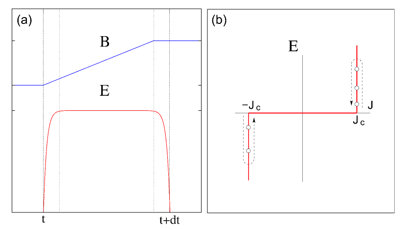
Figure 1.1: (a) Schematic representation the time dependence of the electromagnetic fields within the MQS regime. (b) Pictorial drawing of the critical state model in terms of a one dimensional ${E}({J})$ law.

Notice that, for slow and uniform sweep rates of the external excitations (magnetic field sources and/or transport current), the transient variables $\bf E$, $\bf D$ and $\rho$ are small, and proportional to $\dot{\bf B}$, whereas $\ddot{\bf B}$, $\dot{\bf E}$ and $\dot{\rho}$ are negligible. Thus, the main hypothesis within the MQS regime is that the displacement current densities $\partial_{t}{\bf D}$ are much smaller than $\bf J$ in the bulk and vanish in a first order treatment. This causes a crucial change in the mathematical structure of the Maxwell equations: Ampere’s law is no longer a time evolution equation, but becomes a purely spatial condition. It reads as

$$\nabla\times{\bf B}\simeq\mu_{0}{\bf J}\,,$$ (1.4)

with approximate integrability condition $\nabla\cdot{\bf J}\simeq 0$.

In the MQS limit, Faraday’s law is the unique time evolution equation. Then, one can find the evolution profile ${\bf B}({\bf r},t)$ from

$$\partial_{t}{\bf B}=-\nabla\times{\bf E}=-\nabla\times\left[\rho(\textbf{J})\leavevmode\nobreak\ \mu_{0}\nabla\times{\bf B}\right]\,.$$ (1.5)

Here, $\rho({\bf J})$ plays the role of a nonlinear and possibly nonscalar resistivity that should properly incorporate the physics of the threshold and dissipation mechanisms associated to the flux depinning and flux cutting mechanisms.

We want to mention that, although the B-formulation in Eq. (1.5) is definitely the most extended one, the possibilities of E-formulations [15], J-formulations [16], or a vector potential oriented theory (A-formulation) [17], in which the dependent variables are the fields ${\bf E}$, ${\bf J}$, or A respectively, have also been exploited by several authors.

  1.2 The Critical State Regime And The MQS Limit

In spite of the seeming simplicity of the MQS approach ($\partial_{t}\textbf{D}\approxeq 0$), we want to emphasize that the numerical procedure to solve a critical state problem is closely linked to the consequences of having assumed this limit. Below, two of the most relevant consequences of the MQS limit are highlighted.

1. Notice that, making use of the conductivity law through its inverse function ${\bf E}({\bf J})$, the successive field penetration profiles within the superconductor may be obtained by the finite-difference expression of Faraday’s law,

   $$\frac{B_{l+1}-B_{l}}{\delta t}=-\nabla\times{\bf E}\leavevmode\nobreak\ \left(\mu_{0}\textbf{J}_{l+1}\approx\nabla\times\textbf{B}_{l+1}\right)\,.$$ (1.6)

   Here we have assumed an evolutionary discretization scheme, where $\textbf{B}_{l}$ stands for the local magnetic field induction at the time layer $l\delta t$, and the current density profiles are related to some magnetic diffusion process that takes place when the local condition for critical state $\textbf{J}(\textbf{r})\leq\textbf{J}_{c}(\textbf{r})$ is violated. On the other hand, the constitutive law ${\bf D}({\bf E})$ which is not used in Eq. (1.6), plays no role in the evolution of the magnetic variables $\textbf{B}_{l+1}$ and $\textbf{J}_{l+1}$, which means that the magnetic “sector” is decoupled from the charge density profile because the coupling term (charge recombination) has disappeared. In this sense, notice that the local profile $\textbf{B}_{l+1}$ can be solved in terms of the previous field distribution $\textbf{B}_{l}$ and the boundary conditions at time layer $(l+1)\delta t$.

2. As the initial conditions must fulfill the Ampere’s law $\nabla\times\textbf{B}_{l}=\mu_{0}\textbf{J}_{l}$ as well as $\nabla\cdot\textbf{B}_{l}=0$ and $\nabla\cdot\textbf{J}_{l}=0$, only the inductive component of E (given by $\nabla\times{\bf E}_{\rm ind}=-\dot{\bf B}$, $\nabla\cdot{\bf E}_{\rm ind}=0$) determines the evolution of $\bf B$ (Faraday’s law). At this point, the conducting law in its inverse formulation ${\bf E}({\bf J})$ seems show certain ambiguity, as far as two different material laws related by ${\bf E}_{2}({\bf J})={\bf E}_{1}({\bf J})+\nabla\Phi({\bf J})$ determine the same magnetic and current density profiles. Going into some more detail, whereas for the complete Maxwell equations statement, the potential component of the electric field ($\nabla\times{\bf E}_{\rm pot}=0$, $\epsilon_{0}\nabla\cdot{\bf E}_{\rm pot}=\rho$), is coupled to $\bf B$ and ${\bf E}_{\rm ind}$ through the $\dot{\bf D}$ term (which contains both inductive and potential parts), within the MQS limit it is irrelevant for the magnetic quantities. In fact, one is enabled to include the presence of charge densities without contradiction with the condition $\nabla\cdot{\bf J}\simeq 0$ by means of inhomogeneity or nonlinearity in the $\textbf{E}(\textbf{J})$ relation. Then one has that the condition $\nabla\cdot\textbf{J}=0$ does not imply $\nabla\cdot\textbf{E}=0$. The charge density ${\rho}$ can be understood as a parametrized charge of static character as far as $\dot{\rho}$ is neglected. As indicated above, once the magnetic variables are computed, one has the freedom to modify the “electrostatic sector” if necessary by the rule ${\bf E}({\bf J})+\nabla\Phi$ while still maintaining the values of $\bf B$ and $\bf J$. This invariance can be of practical interest as far as the “electrostatic” behavior in the critical state regime is still under discussion, it because of the inherent difficulties in the direct measurement of transient charge densities [6, 18, 19, 20].

Chapter 2 Variational Theory for Critical State Problems

  2.1 General Principles Of The Variational Method

As we have mentioned before, the numerical solution of the critical state problem from the differential formalism of the Maxwell equations may be cumbersome. One possibility for making the resolution of this system affordable is to find an equivalent variational statement of Eq. (1.6). Then, one can avoid the integration of these set of differential equations by inversion of a set of Euler-Lagrange equations

$$\mu_{0}\textbf{J}_{l+1}-\nabla\times\textbf{B}_{l+1}=0\,,$$ (2.1)

and

$$\mu_{0}\nabla\times\textbf{p}_{l}+\textbf{B}_{l+1}-\textbf{B}_{l}=0\,,$$ (2.2)

for arbitrary variations of the Lagrange multiplier (i.e., $\delta\textbf{p}_{l}$), and the time-discretized local magnetic induction field (i.e., $\delta\textbf{B}_{l+1}$). Eventually, the Lagrange multiplier, $\textbf{p}_{l}$, will be basically identified with the electric field of the problem.

Going into more detail, let us consider a small path step $\delta t$, from some initial profile of the magnetic field $\textbf{B}_{l}(\textbf{r})$ to a final profile $\textbf{B}_{l+1}(\textbf{r})$, and the corresponding $\textbf{J}_{l}(\textbf{r})$ and $\textbf{J}_{l+1}(\textbf{r})$. Defining $\Delta\textbf{B}=\textbf{B}_{l+1}-\textbf{B}_{l}$, both configurations can be considered to be connected by a steady process performing a small linear step, such that $\textbf{B}_{l+1}=\textbf{B}_{l}+s\Delta\textbf{B}$ with $s\in[0,1]\delta t$. Recalling that the initial condition fulfills Ampere’s law $\nabla\times\textbf{B}_{l}=\mu_{0}\textbf{J}_{l}$, as well as $\nabla\cdot\textbf{B}_{l}=0$ and $\nabla\cdot\textbf{J}_{l}=0$, the time-averaged Lagrange density (over whole space) is

$${\cal L}=\frac{1}{2}|\Delta\textbf{B}|^{2}+\textbf{E}\cdot(\nabla\times\textbf{B}_{l+1}-\textbf{J}_{l+1})\delta t\,.$$ (2.3)

Thus, the physically admissible Lagrangian multipliers in the critical state regime must satisfy the condition

$$\textbf{p}=\textbf{E}_{cs}\delta t\,,$$ (2.4)

where the critical state electric field $(\textbf{E}_{cs})$ must be properly defined by the imposed material law $\textbf{E}(\textbf{J})$.

However, concerning the “unknown parameter” $\textbf{J}_{l+1}$, as far as it is not allowed to take arbitrary values, we cannot impose arbitrary variations as it is customary for the typical steady condition of the Euler-Lagrange equations. Instead, an Optimal Control-like Maximum principle equivalent to a maximal projection rule $\textbf{\^{E}}\cdot\textbf{J}$ must be used (see Refs. [7, 21]). For a more comprehensive review of the optimal control theory which can be understood as a generalization of the variational calculus, the interested reader is directed to see, for instance, Refs. [12, 13, 14].

In simple terms, the optimal control concept introduces a geometrical picture of the material law for the boundary conditions of the vector J that may be of much help when discussing the idea of a general critical state theory. Summarizing, it is necessary to declare that there must be a region $\Delta_{\textbf{r}}$ within the J space (possibly oriented according to the local magnetic field B̂, and/or also depending on $|\textbf{B}|$ and r) such that nondissipative current flow occurs when the condition $\textbf{J}\in\Delta_{\textbf{r}}$ is verified. Thus, the minimum of the Lagrangian must be sought within the set of current density vectors fulfilling ${\bf J}\in\Delta_{\textbf{r}}$, i.e.: $\textbf{J}_{l+1}$ is determined by the condition

$${\rm Min}\{{\cal L}\}|_{\textbf{J}\in\Delta_{\textbf{{r}}}}\equiv{\rm Max}\{\textbf{J}\cdot\textbf{p}\}|_{\textbf{J}\in\Delta_{\textbf{{r}}}}\,.$$ (2.5)

Notice that an $\textbf{E}(\textbf{J})$ law is needed in addition to Eq. 2.3. Thus, together with the concept of a very high dissipation when J is driven outside $\Delta_{\textbf{r}}$ by some nonvanishing electric field, Eq. 2.5 suffices to determine the relation between the directions of J and E. Notice that the maximal shielding condition is equivalent to the maximum projection rule, it means that the orthogonality condition of the electric field direction with the surface of $\Delta_{\textbf{r}}$ is recalled, and the Lagrange multiplier can be straightforwardly identified with the electric field of the problem, i.e.,

$${\rm Max}\{\textbf{J}\cdot\textbf{p}\}|_{\textbf{J}\in\Delta_{\textbf{r}}}\equiv{\rm Max}\{\textbf{E}\cdot\textbf{J}\}|_{\textbf{J}\in\Delta_{\textbf{r}}}\,.$$ (2.6)

Notice also that Ampere’s law is imposed [Eq. (2.1)] through the Lagrange multiplier, while the discretized version of Faraday’s law [Eq. (2.2)] is derived as an Euler-Lagrange equation for the variational problem, so that absolute consistency with the Maxwell equations is obtained. In fact, maximal global (integral) shielding is achieved through a maximal local shielding rule [Eq. (2.6)] that reproduces the elementary evolution of $\partial_{t}{\bf J}$ for a perfect conductor with restricted currents. Thus, in practice, if one explicitly introduces Ampere’s law $(\nabla\textbf{B}_{l+1}=\mu_{0}\textbf{J}_{l+1})$, minimization is made in terms of

$${\cal F}[\textbf{J}_{l+1}]={\rm Min}\left\{-\int_{\Re^{3}}\textbf{E}\cdot\textbf{J}_{l+1}\right\}\,,$$ (2.7)

and the minimum is sought over $\textbf{J}_{l+1}\in\Delta_{r}$ for a fixed E. However, as we have mentioned before, special attention must be payed to the feasible ambiguity of the function $\textbf{E}(\textbf{J})$ as it can lead to fake values of the variables J.

Likewise, the straightforward equivalence between the convex functionals for Eqs. (2.5) and (2.7) allows to establish an equivalent minimization principle in terms of the general definitions

$$\textbf{B}=\nabla\times\textbf{A}\,,$$ (2.8)

and

$$\textbf{E}=-\partial_{t}\textbf{A}-\nabla\varPhi\,,$$ (2.9)

by imposing the material law $\textbf{E}(\textbf{J})$ through the Lagrange multiplier $\textbf{p}_{l+1}$. Thus, the minimization problem turns to find out the invariant gauge conditions $\nabla\varPhi_{l+1}$ and $\textbf{J}_{l+1}\in\Delta_{\textbf{r}}$ for a given function $\textbf{A}[\textbf{J}]$, in such manner that

$${\cal F}[\textbf{B}_{l+1},\nabla\varPhi]={\rm Min}\int_{\Re^{3}} \frac{1}{2}|\Delta\textbf{B}|^{2}-\Delta\textbf{A}\cdot(\nabla\times\textbf{B}_{l+1}-\textbf{J}_{l+1})$$

$$-\nabla\varPhi(\nabla\times\textbf{B}_{l+1}-\textbf{J}_{l+1})\delta t\,.$$

We call the readers’ attention to notice that the uncoupling of the electromagnetic potentials can be accomplished by exploiting the arbitrariness involved in the definition of A. In fact, since B is defined through Eq. (2.8) in terms of A, the vector potential is arbitrary to the extent that the gradient of some scalar function can be added. Therefore, the “magnetic sector” could be decoupled of the “electric sector” if the physical admissible states in the time-averaged Lagrange density $L$ are invariant gauge of the Lagrange multipliers p. As a consequence, if the problem is such that there are no intrinsic electromagnetic sources, $\varPhi\equiv 0$ (for type-II superconductors it means absence of transport current), a proper choice of A should satisfy the Coulomb gauge $(\nabla\cdot\textbf{A}\equiv 0)$. In this sense, by using the Laplace equation, the second term in Eq. (2) is reduced to $\Delta\textbf{A}\cdot\delta_{t}^{2}\textbf{A}$ meanwhile the third term have vanished by assuming $\varPhi\equiv 0$. Then, as the MQS approximation relies in assume that the electric field quickly adjusts to a constant value along the interval $[t+\delta t]$, for enough small time steps $\delta t$ (see Fig. 1.1) the action of $\Delta\textbf{A}\cdot\delta_{t}^{2}\textbf{A}$ may be neglected, and therefore the solution of the critical state problem can be also achieved from the functional for the magnetic sector:

$${\cal F}[\textbf{B}(\cdot)]={\rm Min}\int_{\Re^{3}}\frac{1}{2}|\Delta\textbf{B}|^{2}\,.$$ (2.11)

Recall that, the minimization principle is based on a discretization of the path followed by the external sources, meaning that it is an approximation to the continuous evolution whose accuracy increases as the step diminishes.

Moreover, we must emphasize that the derived functionals [Eqs. (2.7) & (2.11)] are in matter of fact fully equivalents, as long as the minimization procedure accomplishes the boundary conditions imposed by the prescribed sources and the material law $\textbf{J}\in\Delta_{\textbf{r}}$. Thus, in those cases when an intrinsic electromagnetic source must be considered, i.e., $\nabla\varPhi\neq 0$, the global set of variables must me constrained by the prescribed conditions. For example, if the superconductor is carrying a transport current $I_{tr}$ flowing through the surface $s$, one has to mandatorily consider the external constraint

$$\int_{s}\textbf{J}\cdot\hat{\textbf{n}}ds=I_{tr}\,$$ (2.12)

and further update the distribution of current to satisfy the physical condition $\textbf{E}\cdot\textbf{J}=0$ (at those points where the magnetic flux does not vary), by means the use of a calibrated potential Ã. Thus, one of the advantage of the formulation in Eq. (2.11) is that the number of variables can be reduced avoiding to include the intrinsic variables associated to $\varPhi$, accordingly to the statement $\textbf{E}=-\partial_{t}\textbf{A}-\nabla\varPhi\equiv\partial_{t}\textbf{\~{A}}$

Concluding, for 3D problems, it must be emphasized that the introduced minimization principle can be applied for any shape of the superconducting volume $\Omega$ as well as for any general restriction (material law) for the current density $\textbf{J}_{l+1}\in\Delta_{\textbf{r}}$. Different possibilities for the material law are described in the following chapter. It is also to be noticed that the searching of the minimum for the allowed set of current densities must fulfill the intrinsic condition $\nabla\cdot\textbf{J}=0$ to be consistent with charge conservation in the quasi-steady regime. Further, from the numerical point of view, the advantage of the variational formulation in Eqs. (2.7) & (2.11) is that one can avoid the integration of the equivalent partial differential equations and straightforwardly minimize the discretized integral by using a numerical algorithm for constrained minimization (see Chapter 3). This fact represents an important advantage in the performance and power of the numerical methods applied to the design of superconducting devices, where symmetry arguments can allow further simplifications and correspondingly faster numerical convergence.

  2.2 The Material Law: SCs with magnetic anisotropy

In this section, we will continue our discussion of the critical state theory which still needs the explicit inclusion of a material law $\textbf{J}(\textbf{E})$ that dictates the magnetic response of a superconducting sample for a given external excitation. For simplicity, we start with an overview of the material law for 1D systems, that will be gradually generalized until a 3D formulation is reached.

2.2.1  Onto The 1D Critical States

For our purposes, it is sufficient to recall that the basic structure of the critical state problem (Fig. 1.1) relates to an experimental graph within the $\{V,I\}$ plane that basically contains two regions defined by the critical current value $I_{c}$ as follows:

1. $-I_{c}\leq I\leq I_{c}$ with perfect conducting behavior, i.e.: $V=0$ and $\partial_{t}I=0$.

2. For $I\gtrsim I_{c}$, the curve is characterized by a high ${\partial_{I}V}$ slope (and antisymmetric for $I\lesssim-I_{c}$). Further steps, with $I$ increasing above the critical value $I_{c}$, i.e., the eventual transition to the normal state, may be neglected for slow sweep rates of the external sources, which produce moderate electric fields.

Within the local description of the electromagnetic quantities involved in the superconducting response, different models have been used for the corresponding $E\leftrightarrow J$ graph, the most popular being

1. The power law model 
   $E=\alpha\;{\rm sgn}(J)\left({|J|}/{J_{c}}\right)^{n}$, with $\alpha$ a constant and $n$ high.

2. The piecewise continuous linear approximation 
   $E=0$ for $|J|\leq J_{c}$, and $E=\beta\;{\rm sgn}(J)(|J|-J_{c})$ for $|J|>J_{c}$, $\beta$ having a high value.

3. Bean’s model 
   $J$ constant for $E=0$, and $J={\rm sgn}(E)J_{c}$ for $E\neq 0$.

In some treatments, the first or second models are implemented, in order to transfer a full ${\bf E}({\bf J})$ law to the Maxwell equations. Further, notice that Bean’s model may be obtained from the other representations through the limiting cases $n\to\infty$ and $\beta\to\infty$ respectively.

The well known experimental evidence of a practical sweep rate independence for magnetic moment measurements (unless for high frequency alternating sources or at elevated temperatures) allows the use of the clearest Bean’s model because the critical state problem is no longer a time-dependent problem, but a path-dependent one, meaning that the trajectory of the external sources ${\bf H}_{0}$ uniquely determines the magnetic evolution of the sample. This makes an important difference when one compares to more standard treatments, as far as Faraday’s law is not completely determined from the path [4]. Strictly speaking, one has

$$\Delta{\bf B}=-\nabla\times[{\bf E}\Delta t]\,\,,$$ (2.13)

with $\Delta t$ (and therefore $|{\bf E}|$) depending on the external sources. i.e., the absence of an intrinsic time constant gives way to the arbitrariness in the time scale of the problem.

Furthermore, in the actual 1D applications of Beans’s model, Faraday’s law is not strictly solved and E is absent from the theory. It is just the sign rule (the vectorial part of the material law), that is used to integrate Ampere’s law. Notice that such sign rule corresponds to a maximal shielding response against magnetic vector variations, and thus, determines the selection of $J=\pm J_{c}$.

Regarding the direction of E, in “1D” problems one has ${\bf J}\parallel{\bf E}$ and both orthogonal to $\bf B$, such that the physical threshold related to a maximum value of the force balancing the magnetostatic term ${\bf J}\times{\bf B}$ gives place to the material law

$$J_{\perp}={\rm sgn}(E_{\perp})J_{c\perp}\qquad{\rm for}\qquad E_{\perp}\neq 0\,\,.$$ (2.14)

Here, $E_{\perp}$ stands for the component of ${\bf E}$ along the direction ${\bf B}\times({\bf J}\times{\bf B})$, and the material law falls in a “1D” scalar condition which describes the physical mechanism of vortex depinning.

At this point, the constitutive relation for the critical state describes the underlying physics for the coarse-grained fields in homogeneous type-II superconductors. However, it is well known that the coarse-grained behavior approach straightforwardly depends on the manufacturing process of the superconducting sample as far as inclusion of impurities, magnetic defects, or deformation of their cristal structure imposes the local coupling of $J_{c}$ with the intrinsic variation of the magnetic field B. Thus, for practical purposes we emphasize that the theoretical framework developed in this book is fully general, with caution of suggest to the experimentalist the need of an apriori measurement of the dependence $\textbf{J}_{c}[\textbf{r},\textbf{B},T]$ at least in those cases where the condition $\textbf{J}\perp\textbf{B}$ can be asserted. Henceforth, the implementation for a particular superconductor can be carried out.

2.2.2  Towards The 3D Critical States

In the case of superconductors with anisotropy of the critical current, the description of their magnetic behavior requires the development of approaches more sophisticated than 1D-Bean’s model. The main issue is that, in general, the parallelism of ${\bf E}$ and ${\bf J}$ and their perpendicularity to ${\bf B}$ are no longer warranted. Then, the sign rule of Eq. (2.14) does not suffice for determining the solution of Eq. (2.6), and the optimal control condition with $\textbf{J}\in\Delta_{\textbf{r}}$ (a vectorial rule) must be invoked.

The simplest assumption that translates the critical state problem to 3D situations was already issued by Bean in Ref. [22]. It has been called the isotropic critical state model (ICSM) and generalizes 1D Bean’s law to

$${\bf J}=J_{c}\,\hat{\bf E}\quad{\rm if}\quad E\neq 0\,,$$ (2.15)

i.e., the region $\Delta_{\textbf{r}}$ becomes a sphere. Noticeably, in spite of lacking a solid physical basis, thanks to its mathematical simplicity, this qualitative model has been widely used by several authors for reproducing a number of experiments with rotating and crossed magnetic fields [7, 8, 23]. In any case, one could argue that statistical averaging over a system of entangled flux lines within a random pinning structure might be responsible for the isotropization of $\Delta_{\textbf{r}}$.

On the other hand, the general statement of the critical state in terms of well accepted physical basis was firstly introduced by John R. Clem [3], and it is currently known as the double critical state model (DCSM). In particular, this theory assumes two different critical parameters, $J_{c\parallel}$ and $J_{c\perp}$ acting as the thresholds for the components of ${\bf J}$ parallel and perpendicular to ${\bf B}$ respectively. Notice that, $J_{c\perp}$ relates to the flux depinning threshold induced by the Lorentz force on flux tubes ($\textbf{J}\times\textbf{B}$), while the additional $J_{c\parallel}$ is imposed by a maximum gradient in the angle between adjacent vortices ($\textbf{B}\cdot\nabla\gamma=J_{\parallel}$) before mutual cutting and recombination occurs [see Fig. 2.1 (a)]. In brief, the DCSM may be expressed by the statement

$$\left\{\begin{array}[]{ll}{\bf J}_{\parallel}&=J_{c\parallel}\;\hat{\bf u}\\ {\bf J}_{\perp}&=J_{c\perp}\,\hat{\bf v}\end{array}\right.\,,$$ (2.18)

being û the unit vector for the direction of B, and v̂ a unit vector in the perpendicular plane to B.

Within the DCSM, the region $\Delta_{\textbf{r}}$ is a cylinder with its axis parallel to $\bf B$, and a rectangular longitudinal section in the plane defined by the unit vectors $\hat{\bf B},\hat{\bf J}_{\perp}$ [see Fig.  2.1 (b)]. The edges of the region $\Delta_{\textbf{r}}$ introduce a criterion for classifying the CS configurations into:

1. T zones or flux transport zones ($J_{\perp}=J_{c\perp}$; $J_{\parallel}<J_{c\parallel}$) where the flux depinning threshold has been reached (${\bf J}$ belongs to the horizontal sides of the rectangle),

2. C-zones or flux cutting zones ($J_{\parallel}=J_{c\parallel}\leavevmode\nobreak\ ;\leavevmode\nobreak\ J_{\perp}<J_{c\perp}$) where the cutting threshold has been reached (${\bf J}$ belongs to the vertical sides of the rectangle),

3. CT zones ($J_{\parallel}=J_{c\parallel}$ and $J_{\perp}=J_{c\perp}$) where both $J_{\parallel}$ and $J_{\perp}$ have reached their critical values (corners of the rectangle), and

4. O zones depicted the regions without energy dissipation (the current density vector belongs to the interior of the rectangle).

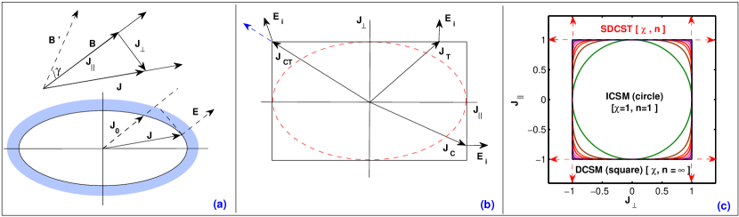
Figure 2.1: Pane (a), Top: Schematic representation of the local relative orientations of B and J. Also sketched is the direction of the magnetic field at some neighboring point, at an angle $\gamma$. The vectors ${\bf B}$, ${\bf B}^{\prime}$ and ${\bf J}$ do not necessarily lie at the same plane. The current is decomposed into its parallel and perpendicular components, i.e.: ${\bf J}={\bf J}_{\parallel}+{\bf J}_{\perp}$. Bottom: the perfect conducting region within the plane perpendicular to B. An induced electric field is shown. Initially (${\bf J}_{0}$), the high dissipation region is touched, but almost instantaneously J shifts along the boundary, reaching a point where the condition ${\bf E}\perp\partial\Delta_{\textbf{r}}$ is fulfilled. Anisotropy within the plane is allowed. Pane (b): Geometric interpretation of the DCSM. J is constrained to the boundary of a rectangular region. T, C and CT states are related to the horizontal and vertical sides, and to the corners. Coupling between the components $J_{c\parallel}$ and $J_{c\perp}$ is envisaged by the EDCSM (dotted red ellipse). Pane (c): Our generalization of the material law for critical state problems or SDCST. Several regions are shown from the degree of the superelliptical functions ($n=1,2,3,4,6,10,20,40,\infty$) and $\chi=J_{c\parallel}/J_{c\perp}=1$.

Notice that $J_{c\parallel}$ and $J_{c\perp}$ are determined from different physical phenomena, and their values may be very different (in general $J_{c\parallel}>J_{c\perp}$ or even $J_{c\parallel}\gg J_{c\perp}$). Nevertheless, the coupling of parallel and perpendicular effects has been longer recognized by the experiments [20, 24] and, for instance, may be included in the theory by the condition $J_{c\parallel}=KBJ_{c\perp}$ with $K$ a material dependent constant.

Recalling that the mesoscopic parameters $\textbf{J}_{c}$ are related to averages over the flux line lattice, interacting activation barriers for the mechanisms of flux depinning and cutting are expected and this may give place to deformations of the boundary $\partial\Delta_{\textbf{r}}$ [see Fig.  2.1(b)]. Thus, validated in those cases where a good agreement with the experiments is achieved, the theoretical scenario can be enlarged by a number of alternative approaches that focus on different aspects of the vast number of experimental activities in this field, e.g. one can identify the so-called:

1. Isotropic critical state models (ICSM) [4, 5, 23]
                                 $J^{2}=J_{\parallel}^{2}+J_{\perp}^{2}\leq J_{c}^{2}$

2. Elliptical double critical state models (EDCSM) [4, 25]
                                $J_{\parallel}^{2}/J_{c\parallel}^{2}+J_{\perp}^{2}/J_{c\perp}^{2}\leq 1$

3. T critical state model (TCSM) [4, 5, 6, 26, 27]
                             $J_{\parallel}$ unbounded $\forall$ $J_{\perp}\leq J_{c\perp}$ .

Remarkably, the whole set of models have been recently unified by us in Ref. [5] within a continuous two-parameter theory that poses the critical state problem in terms of geometrical concepts within the $J_{\parallel}-J_{\perp}$ plane (see Fig.  2.1 (c)). To be specific, in this framework, we have shown that by the application of our variational statement [4], one is able to specify almost any critical state law by means of an integer index $n$, that accounts for the smoothness of the $J_{\parallel}(J_{\perp})$ relation, and a certain bandwidth characterizing the magnetic anisotropy ratio $\chi\equiv J_{c\parallel}/J_{c\perp}$. This and the variational formalism introduced above constitutes the so-called Smooth Double Critical State Theory (SDCST), which allows to elucidate the relation between diverse physical processes and the actual material law.

Mathematically, the material law introduced in our general theory for the critical state problem or SDCST is based upon the idea that either material or extrinsic anisotropy can be easily incorporated by prescribing a region $\Delta_{\textbf{r}}$ where the physically admissible states of J are hosted as limiting cases of a smooth expression defined by the two-parameter family of superelliptic functions,

$$\left(\frac{J_{\parallel}}{J_{c\parallel}}\right)^{2n}+\left(\frac{J_{\perp}}{J_{c\perp}}\right)^{2n}\leq 1.$$ (2.19)

We call the readers’ attention to the fact that an index $n=1$ and a bandwidth defined by $\chi\equiv J_{c\parallel}/J_{c\perp}=1$ correspond to the standard ICSM [23]. On the other hand, when one assumes enlarged bandwidth (i.e.: $\chi>1$), the region $\Delta_{\textbf{r}}$ of the SDCST becomes the standard EDCSM introduced by Romero-Salazar and Pérez-Rodríguez [25]. When the bandwidth $\chi$ is extremely large, i.e., $J_{c\parallel}\gg J_{c\perp}$, one recovers the so-called $T-$zones treated by Brandt and Mikitik [26]. Rectangular regions strictly corresponding to the DCSM [3] are obtained for the limit $n\rightarrow\infty$ and arbitrary $\chi$. Finally, allowing $n$ to take values over the positive integers, a wide scenario describing anisotropy effects is envisioned [Fig. 2.1(c)]. Such regions will be named after superelliptical and their properties can be understood in terms of the rounding (or smoothing) of the corners for the DCSM.

Chapter 3 Computational Method

In chapter 2.1 we have mentioned that the minimization functionals [Eq. (2.7) or Eq. (2.11)] may be transformed so as to get a practical vector potential formulation. In turn, the resulting formulation can be expressed in terms of the so-called magnetic inductance matrices which allows a clearest identification of the set of elements playing some role in the minimization procedure. In this chapter, we shall discuss how to implement the above statements for general critical states in the framework of the computational methods for large scale nonlinear optimization problems.

Being more specific, in Eq. (2.11) the integrand $\frac{1}{2}(\Delta{\bf B})^{2}$ can be rewritten as $\frac{1}{2}(\Delta{\bf B})\cdot(\nabla\times\Delta{\bf A})$, and manipulated to get $\frac{1}{2}(\Delta{\bf A})\cdot(\nabla\times\Delta{\bf B})$ plus a divergence term, fixed by the external sources at a distant surface. Now, the integral is restricted to the superconducting sample volume $\Omega$, because $\nabla\times\Delta{\bf B}=\mu_{0}\Delta{\bf J}$ is only unknown within the superconductor. In addition, assuming that local sources such as an injected transport current may be introduced as an external constraint, and with the boundary condition that A goes to zero sufficiently fast as they approach infinity, the vector potential can be expressed as:

$$\Delta{\bf A}=\Delta{\bf A}_{0}+\frac{\mu_{0}}{4\pi}\int_{\Omega}\frac{\Delta{\bf J}}{|{\bf r}-{\bf r}^{\prime}|}d^{3}{\bf r}^{\prime}\,.$$ (3.1)

This transforms ${\cal F}$ into a double integral over the body of the sample, i.e.:

$${\cal F}[\textbf{A}(\cdot),J\in\Delta_{\textbf{r}}]= \frac{8\pi}{\mu_{0}}\int_{\Omega}\Delta{\bf A}_{0}\cdot{\bf J}_{l+1}({\bf r})d^{3}{\bf r}$$ (3.2)

$$+\int\!\int_{\Omega\times\Omega}\frac{{\bf J}_{l+1}({\bf r}^{\prime})\cdot[{\bf J}_{l+1}({\bf r})-2{\bf J}_{l}({\bf r})]}{|{\bf r}-{\bf r}^{\prime}|}d^{3}{\bf r}d^{3}{\bf r}^{\prime}\;$$

As a consequence, only the unknown current components within the superconductor $(\textbf{J}_{l+1})$ appear in the computation so reducing the number of unknown variables. At this point let me emphasize that Eq. (3.2) can be applied for any shape of the superconducting volume $\Omega$ as well as for any physical constraint (material law $\Delta_{\textbf{r}}$) for the local current density $\textbf{J}_{l+1}$, and further for any condition defined by the external sources ($\textbf{A}_{0}$). Above this, minimization must ensure the charge conservation condition by searching the minimum for the allowed set of current densities fulfilling $\nabla\cdot\textbf{J}=0$.

On the other hand, also it may be noticed that the double integral in Eq. (3.2) can be (eventually) identified as the Neumann formula once it has been transformed into filamentary closed circuits. A noteworthy fact is that regarding the superconducting volume, the coefficients of the intrinsic inductance matrices are straightforwardly independent of time and consequently, they appear in the root problem before going to minimize the functional. Indeed, the proper description of the inductance coefficients directly depends on the geometry of the superconductor and the boundary conditions defined by the dynamics of the external electromagnetic sources, where any symmetry of the problem allows further simplifications and correspondingly faster numerical convergence. To be specific, upon discretization in current elements ($I_{i}=J_{i}s_{i}$), the minimization functional for critical state problems bears the algebraic structure

$${\cal F}[I_{l+1}]=\frac{1}{2}\sum_{i,j}I_{i,l+1}M_{ij}I_{j,l+1}-\sum_{i,j}I_{i,l}M_{ij}I_{j,l+1}+\sum_{i}I_{i,l+1}\Delta A_{0}(M_{0})\,,$$ (3.3)

with $\{I_{i,l+1}\}$ the set of unknown currents at specific circuits for the problem of interest, $M_{ij}$ their intrinsic inductance coupling coefficients, and $M_{0}$ the inductance matrices associated to the external sources $A_{0}$.

Corresponding to the critical state rule ${\bf J}\in\Delta_{\textbf{r}}$, in order to minimize Eq. (3.3) each value $J_{i}$ must be constrained. Thus, as it was described in chapter 2.2.2, we have found that a number of constraints related to physically meaningful critical state models may be expressed in the algebraic form

$${\rm F}_{\alpha}\left(\sum_{i}I_{i}C_{ij}^{\alpha}I_{j}\right)\leq f_{0\alpha}\,\leavevmode\nobreak\ \forall\leavevmode\nobreak\ j$$ (3.4)

with $f_{0}$ some constant representing the physical threshold, and ${\rm F}_{\alpha}(\cdot)$ an algebraic function based upon a coupling matrix $C_{ij}^{\alpha}$ whose elements depend on the physical model. For example, in the simpler cases (isotropic models), the constraints correspond to assume the matricial elements $C_{ij}=\delta_{ij}$, and the physical threshold $f_{0}={J}_{c}^{2}$.

For simplicity, most technical procedures related to the introduction of intricate models and either depict the minimization functional in terms of the inductance coefficients (including those for external sources) will be left as matter of study of the following chapters (Part II). In return, below we present a thorough analysis of the computational tools handled for critical state problems at large scale.

With the purpose of obtaining a minimal understanding about how a critical state problem can be tackled from the numerical point of view, the computational method is sketched in the flow charts of figures 3.1 & 3.2.

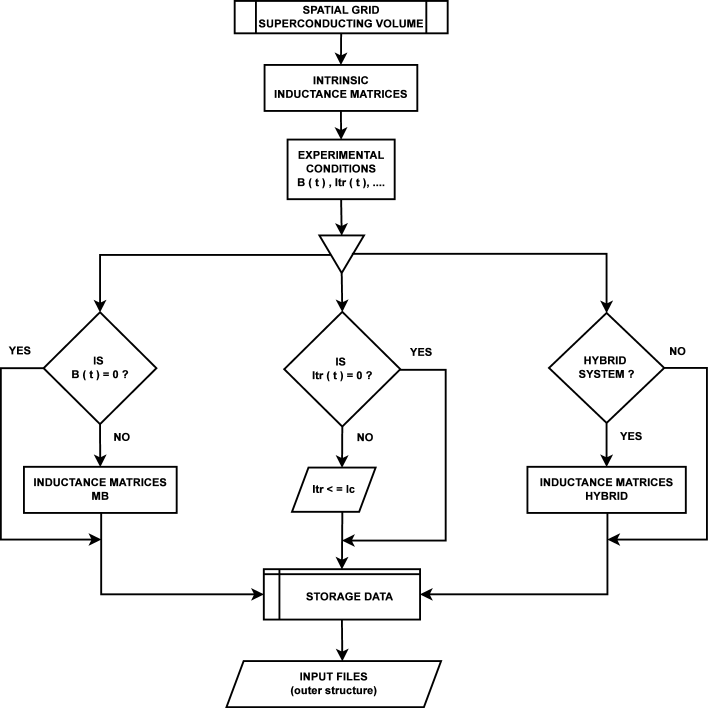
Figure 3.1: Flow chart describing the preparation and management of the input elements for the objective function.

The first step is designing a grid which will allows to describe the superconducting volume $\Omega$ as a set of elements $\delta\Omega_{i}$, each of them characterized by a well defined current density flowing along the coordinates $\textbf{r}_{i}$. Then, the matrices for the intrinsic inductance coefficients between the elements $\textbf{J}(\textbf{r}_{i})$ and $\textbf{J}(\textbf{r}_{j})$ for all the set of possible couples $(\textbf{r}_{i},\textbf{r}_{j})\in\Omega$ must be calculated and stored on disk. As the mesh of points $(\textbf{r}_{i},\textbf{r}_{j})$ can be considerably large, we suggest take advantage on the matricial formalism provided by Matlab^® and their own language for storage data. Once the spatial elements playing some role into the functional have been properly defined, the temporal sector must be introduced by means enough small path steps of the external electromagnetic sources, i.e., the experimental conditions must be connected by the finite difference expressions such a $\Delta\textbf{B}_{0}=\textbf{B}_{l+1}-\textbf{B}_{l}$, where the associated distribution of currents $\textbf{I}_{l+1}$ plays the role of unknown. To be specific, in those cases where the superconductor is subjected to an external magnetic field $\textbf{B}_{0}$, additional inductance matrices ($M_{0}$) must be introduced according to the definition

$$\textbf{A}_{0}(\textbf{B}_{0},\textbf{r}_{j})=\textbf{B}_{0}\times\textbf{r}_{j}\,.$$ (3.5)

On the other side, the vector potential $\textbf{A}_{0}$ not only allows to define the contribution at the local potential A produced by an external magnetic field ($\textbf{A}_{{\rm B}}$), rather it also allows consider the coupling with another materials such as ferromagnets.

Before going within the minimization procedure, it has to be noticed that those cases considering a transport current along the superconducting sample must be understood as a problem where the minimization variables are required to satisfy a set of auxiliary constraints [see Eq. (2.12)] under the global critical state condition $I_{tr}\leq I_{c}$. Also, as the values for the elements $\textbf{I}_{l}(\textbf{r})$ are assumed to be known in advance, the linear elements into the argument of the functional (objective function) can be calculated before minimizing.

At this point, it is probably worthwhile to argue on what we mean by the computational method for minimization of an objective function. Firstly, this notion is clearly computer dependent, as the size of large scale problems can require a substantial amount of memory and store. Moreover, what is large in a personal computer can be significantly different from what is large on a super computer. The first machine just to have a smaller memory and storage than the second one, and therefore has more difficulty handling problems involving a large amount of data. Secondly, the size of the objective function strongly depends on the structure and the mathematical formulation of the problem and exploiting it is often crucial if one wants to obtain an answer efficiently. The complexity of this structure is often a central key in assessing the size of a problem. For example, for linear objective functions (not our case) it is possible to solve pretty large size problems (say four million variables). However, the objective function for problems in applied superconductivity is in general highly nonlinear and, for instance, the quadratic terms suggest to reduce the number of variables in a root square factor (say two thousand variables). One advisable possibility for reducing the number of elements in the objective function is subdividing the problem into loosely connected subsystems, i.e., all the internal operations which do not depend of the minimization variables must be preallocated to a well structured data (Figure. 3.1). Lastly, an efficient algorithm for nonlinear optimization problems must be either invoked or built. Fortunately, nowadays there is a significant amount of available software with standard optimization tools which allow a faster foray in this matter [28, 29].

We must call reader’s attention on the fact that efficient algorithms for small-scale problems (in the sense that, assuming infinite precision, quasi-Newton methods for unconstrained optimization are invariant under linear transformations) do not necessarily translate into efficient algorithms for large scale problems. Perhaps the main reason is that, in order to be able to handle large problems with a high accuracy, the structure of the objective function and the minimization algorithms have both of them to be enough simple and tractable to avoid a wasting of time in the scaling of variables for the inner iteration subproblem (the minimization itself) and the finding of an optimum value for each one of the variables with respect to the remaining variables sought. In this context, one of the most powerful algorithms for large and nonlinear constrained optimization problems, known as LANCELOT, has been developed by the professors Andrew Conn (IBM corporation, USA), Nick Gould (Rutherford Appleton Laboratory, UK), Philippe Toint (Facultés Universitaries Notre-dame de la Paix, Belgium), and Dominique Orban (Ecole Polytechnique de Montreal, Canada) [29]. The wide number of optimization techniques provided by this package and their flexibility in handle and storage of large amounts of variables, make this program a clever choice for tackle highly complicated systems as those described by Eq. (3.2).

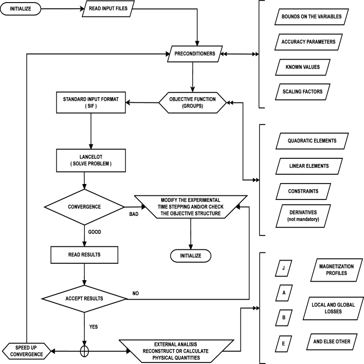
Figure 3.2: Flow chart describing the main structure of the computational method implemented along this book.

A thorough study of the minimization techniques and the computational language allocated in this package is far away of the purpose of this thesis. However, the structure of a general problem can be understood via the flow chart in figure 3.2. In brief, the minimization functional is translated into a suite of FORTRAN procedures for minimizing an objective function, where the minimization variables are required to satisfy a set of auxiliary constraints and possibly internal bounds. Here, the major advantage of LANCELOT is the use of a Standard Input Format (SIF) as a unified method for communicating numerical data and FORTRAN subprograms with any optimization algorithm. Thus, when an optimization problem (minimizing or maximizing a sought of variables) is specified in the SIF decoder, one is required to write one or more files in ordered sections which accomplish the role of introduce the set of preconditioners for the objective function.

Once the set of input data has been structured accordingly to the number of variables and further on the temporal dependence of the experimental conditions (see Fig. 3.1), one is enabled to predefine a set of input cards allowing the knowledgeable user to specify a priori known limits on the possible values of the objective function, as well as on the specific optimization variables, accuracy parameters, and scaling factors (see Fig. 3.2). Then, the minimization functional or so-called objective function is subdivided in a set of groups, whose purpose is twofold: On the one hand, the linear and nonlinear (quadratic) elements for the minimization procedure are identified in a fore. Likewise, the specification of analytical first derivatives is optional, but recommended whenever possible. The SIF decoder allows also include the Hessian matrix of the objective function, if the second-order partial derivatives of the whole set of minimization variables are known, otherwise the derivatives of the nonlinear element functions can be approximated by some finite difference method.

Actually, the full Hessian matrix can be difficult to compute in practice; in such situations, quasi-Newton algorithms can be straightforwardly called by LANCELOT where at least ten different minimization algorithms have been already implemented and coded according to the standard input format provided by the SIF decoder [29]. Notwithstanding, the solution obtained by LANCELOT may be compromised if finite difference approximations are used, it has been our experience that, once understood, the programming language of SIF is in fact quite efficient for problem specifications, in such manner that for objective functions correctly written, and constraint functions well defined, any method can efficiently reach to the solution sought. In this sense, additional groups may be announced to make up the objective function by including an “starting point” for the envisaged solution (if it is more or less known, or by defect it is equals to zero) or, for introducing additional constraints (external functions conditioning the system) as it is the case when the superconductor implies a flow of transport current.

It may happen that a specific problem uses variables or general constraints whose numerical values are widely different in magnitude, causing significant difficulties in the numerical convergence. However, LANCELOT also gives the chance of incorporate a list of scaling factors which are applied to the general constraints and variables separately before the optimization commences, allowing a clearest handling of the group elements in highly nonlinear problems as those herein considered. Thus, assuring a good convergence, whether single or double precision, is implying in turn to modify the experimental time stepping and either, the accuracy parameters such as, the number of iterations allowed, the constraint and gradient accuracy, the penalty parameter and the trust region for the optimizing.

Finally, in applied superconductivity, a set of complementary programs have to be developed in an effort to provide a comprehensive understanding of the temporal evolution of the electromagnetic quantities. For example, if the set of minimization variables corresponds to the local profiles of current density $\textbf{J}_{i}(\textbf{r}_{i})$, additional codes must to be used for calculating $\textbf{A}_{i}(\textbf{r})$, $\textbf{B}_{i}(\textbf{r})$, and $\textbf{E}_{i}(\textbf{r})$ in the whole $\Re^{3}$-space. Thus, although integrated quantities such as the magnetic moment $\textbf{M}(\textbf{J}_{i},\textbf{r}_{i})$ may be revealing a smooth trend despite the use of a poor numerical accuracy, it is of utter importance testing the numerical convergence by calculating the local profiles for the electromagnetic quantities concerning to derived quantities. In this sense, the following part of this book is devoted to the reliable solution of some interesting problems in applied superconductivity, where the critical state statement falls into a large scale optimization problem.

Conclusions I

In summary, in this part we have shown that the critical state theory for the magnetic response of type-II superconductors may be built in a quite general framework and in turn it may be solved by several means. As our interest is to deal with highly nonlinear problems at large-scale, we have emphasized in the performance of variational methods and computational techniques for solving problems on personal computers.

We remark that the basic concepts underlying our generalization of the critical state theory can be identified as follows:

1. The critical state theory bears a Magneto Quasi Steady (MQS) approximation for the Maxwell equations in which $\ddot{\textbf{B}}$, $\dot{\bf E}$ and $\dot{\rho}$ are second order quantities and consequently, the displacement current densities $\dot{\textbf{D}}$ are much smaller than J in the bulk and vanish in a first order treatment. This means that the magnetic flux dynamics can be entirely described by the finite-difference expression of Faraday’s law

   $$\Delta\textbf{B}=-\nabla\times(\textbf{E}\delta t)\,,$$ (3.6)

   where the physically admissible states must accomplish the MQS Ampere’s law, i.e., $\nabla\times\textbf{B}=\mu_{0}\textbf{J}$. Here, the inductive part of ${\bf E}$ may be introduced through Faraday’s law, whereas the role of electrostatic quantities is irrelevant for the magnetic sector. In other words, E may be modified by a gradient function (${\bf E}\to{\bf E}+\nabla\phi$) with no effect on the magnetic response.

2. In type-II superconductors, the law that characterizes the conducting behavior of the material may be written in terms of thresholds values for the current density constrained to a geometrical region $(\textbf{J}\in\Delta_{\textbf{r}})$ which suffices to determine the relation between the directions of E and J. Thus, E is no longer an unknown variable but rather plays the role of a parameter to be adjusted in a direct algebraic minimization, i.e.,

   $${\rm Min}\{L\}|_{\textbf{J}\in\Delta_{\textbf{{r}}}}\equiv{\rm Max}\{\textbf{J}\cdot\textbf{p}\}|_{\textbf{J}\in\Delta_{\textbf{{r}}}}\equiv{\rm Max}\{\textbf{E}\cdot\textbf{J}\}|_{\textbf{J}\in\Delta_{\textbf{{r}}}}\,.$$ (3.7)

   In physical terms, the material “reacts” with a maximal shielding rule when electric fields are induced, and a perfect conducting behavior characterizes the magnetostatic equilibrium when external variations cease. In fact, is to be noticed that the above representation can be understood as the macroscopic counterpart of the underlying vortex physics. Thus, recalling that, in type II superconductors an incomplete isotropy for the limitations of the current density relative to the orientation of the local magnetic field arises from the different physical conditions of current flow either along or across the Abrikosov vortices, one may talk about magnetically induced anisotropy where the physical barriers of flux depinning and cutting are customarily depicted by the condition $\textbf{J}\leq\textbf{J}_{c}\in\Delta_{\textbf{r}}$. The evolution from one magnetostatic configuration to another occurs through the local violation of this condition, i.e.: ${\bf J}\notin\Delta_{\textbf{r}}$ ($\textbf{J}>\textbf{J}_{c}$). However, owing to the high dissipation, an almost instantaneous response may be assumed, represented by a maximum shielding rule in the form ${\rm Max}\{{\bf J}\cdot\hat{\bf E}\}\left.\right|_{{\bf J}\in\Delta_{\textbf{r}}}$.

3. With the aim of offering a meaningful reduction of the number of variables, we have shown that the problem can be simplified by solving a minimization functional with a underlying structure based upon inductance matrices [see Eq. (3.3)]. In particular, the mutual inductance representation with ${\bf J}({\bf r})$ as the unknown, offers two important advantages:

   (i) intricate boundary conditions and infinite domains are avoided, and

   (ii) the transparency of the numerical statement and its performance (stability) are outlined.

   Then, the quantities of interest (flux penetration profiles and magnetic moment) are obtained by integration.

4. Most popular models for critical state problems have been generalized in our so-called smooth double critical state theory (SDCST) for anisotropic material laws [5]. This theory relies on our variational framework for general critical state problems [4] that allows us to incorporate the above-mentioned physical structure in the form of mathematical restrictions for the circulating current density. Two fundamental material-dependent quantities play key roles in this theory $(J_{c\parallel},J_{c\perp})$ related to the flux cutting and flux depinning thresholds. Notoriously, the boundary condition for the material law $\textbf{J}\in\Delta_{\textbf{r}}$ and the mutual interaction between the critical thresholds have been described in a quite general picture, based upon the relation between the coupling parameters $\chi\equiv J_{c\parallel}/J_{c\perp}$ and the smoothing index $n$ of the superelliptical condition $(J_{\parallel}/J_{c\parallel})^{2n}+(J_{\perp}/J_{c\perp})^{2n}\leq 1$.

   Hence, our SDCST cover a wide range of laws:

   (i) the isotropic model ($\chi^{2}=1$, $n=1\Rightarrow\Delta_{\textbf{r}}$ is a circle),

   (ii) the elliptical model ($\chi^{2}>1$, $n=1\Rightarrow\Delta_{\textbf{r}}$ is an ellipse),

   (iii) the rectangular model ($\chi^{2}\geq 1$, $n\to\infty\Rightarrow\Delta_{\textbf{r}}$ is a rectangle),

   (iv) the infinite band model ($\chi^{2}\rightarrow\infty$), and

   (v) else others with smooth magnetic anisotropy ($\chi^{2}\geq 1$, $n\in{\rm N}\geqslant 1\Rightarrow\Delta_{\textbf{r}}$ is a rectangle with smoothed corners).

Finally, let me emphasize that the scope of our theory is rather beyond the actual examples treated in the following part of this thesis. On the one side, we have shown that the critical state concept allows arbitrariness in the presence of electrostatic charge and potential, and one could simply upgrade the models by the rule ${\bf E}\to{\bf E}+\nabla\phi$ if necessary. For instance, a scalar function $\phi$ may be introduced if the direction of ${\bf E}$ has to be modified respect to the maximum shielding rule in the MQS limit. On the other side, the extension of the theory to arbitrary sample geometries is intrinsically allowed by the mutual inductance representation. Thus, this first part has laid necessary groundwork for attacking general critical state problems in 3D geometry.

Part II Critical State Problems:

Effects & Applications

      Introduction

In the first part of this book the magnetic flux dynamics of type-II superconductors within the critical state regime has been posed in a generalized framework, by using a variational theory supported by well established physical principles and quite general numerical methods. The equivalence between the variational statement and more conventional treatments, based on the solution of the differential Maxwell equations together with appropriate conductivity laws have been stated. On other side, in an effort to explore new physical scenarios devoted to convey the advantages of the variational statement, in this part we present a thorough analysis of several problems of recognized importance for the development and physical understanding of intrinsic phenomena linked to the technological application of type-II superconductors.

In particular, Chapter 4 is devoted to present the extensions of the so-called double critical state model to three dimensional configurations in which either flux transport (T-states), cutting (C-states) or both mechanisms (CT-states) occur. Firstly, we show the features of the transition from T to CT states. Secondly, we focus on our generalized expression for the flux cutting threshold in 3D systems and show its relevance in the slab geometry. Recall that, our method has allowed us to unify a number of conventional models describing the complex vortex configurations in the critical state regime. Thus, in this chapter several material laws already included in our generalized SDCST are compared to each other so as to weigh out the inherent influence of the magnetic anisotropy and the coupling between the flux depinning and cutting mechanisms. This is done by using different initial configurations (diamagnetic and paramagnetic) of a superconducting slab in 3D magnetic field, which allow to show that the predictions of the SDCST range from the collapse to zero of transverse magnetic moment in the isotropic model to nearly force-free configurations in which paramagnetic values can arbitrarily increase with the applied field for magnetically anisotropic current-voltage laws.

Chapter 5 addresses the study of several intriguing phenomena for the transport current in type II superconductors. In particular, we present an exhaustive study of the electromagnetic response for the so-called longitudinal transport problem (current is applied parallel to the external magnetic field) in the slab geometry. On the one hand, we will introduce a simplified analytical model for a 2D configuration of the electromagnetic quantities. Then, based upon numerical studies for general scenarios (3D) we will go beyond the analytical models, and in general, it will shown that a remarkable inversion of the current flow in a surface layer may be predicted under a wide set of experimental conditions, including modulation of the applied magnetic field either perpendicular or parallel (longitudinal) to the transport current density. On the other hand, according to our SDCST where the magnetic anisotropy of the superconducting material obeys a geometrical region enclosed by a superelliptical function for the current density vector, a thorough characterization of the underlying mechanism of flux cutting and depinning has been performed. Thus, the intriguing occurrence of negative current patterns and the enhancement of the transport current flow along the center of the superconducting sample are reproduced as a straightforward consequence of the magnetically induced internal anisotropy. Moreover, we establish that the maximal transport current density allowed by the superconducting sample after compression towards the center of the sample, is related to the maximal projection of the current density vector onto the local magnetic field or material law. Also, it will be shown that a high correlation exists between the evolution of the transport current density and the appearance of striking collateral effects, such as local and global paramagnetic structures in terms of the applied longitudinal magnetic field. Finally, the elusive measurement of the threshold value for the cutting current component ($J_{c\parallel}$) is suggested on the basis of local measurements of the transport current density.

Finally, chapter 6 is devoted to introduce a thorough study of the electromagnetic response, either local or global, of straight infinite superconducting wires in the critical state regime under the action of diverse configurations of transverse magnetic field and/or longitudinal transport current. A comprehensive theoretical framework for the physical concepts underlying the temporal evolving of the electromagnetic quantities and the production of hysteretic losses is in a fore. Thus, along this line, and for the numerical implementation of our numerical statement, we have considered three different excitation regimes which are focused on the electromagnetic response of a superconducting wire with cylindrical cross-section: (i) Isolated electromagnetic excitations, in which only the action of an external source of oscillating transverse magnetic field, $\textbf{B}_{0}$, or an impressed AC transport current, $I_{tr}$, is conceived. (ii) Synchronous oscillating excitations, which deals with the simultaneous action of $\textbf{B}_{0}$ and $I_{tr}$ for experimental situations wherein both sources are showing the same oscillating features (identical phase and frequency). Eventually, in (iii) asynchronous excitation sources, we have addressed to most intricate configurations where the oscillating sources are out of phase by assuming that one of them sources is connected to a power supply with a double frequency than the other. The temporal dynamics of the assorted electromagnetic quantities, such as the local profiles of current density $\textbf{J}_{i}$, the lines of magnetic field (isolevels of the vector potential A), the vector components of the magnetic flux density B, the local density of power dissipation $\textbf{E}_{i}\cdot\textbf{J}_{i}$, the magnetic moment curves M, and the hysteretic AC losses $L$, are shown for each one of the above mentioned cases including a wide set of amplitudes for the oscillating excitations. Striking differences between the actual hysteretic losses (predicted by numerical methods) and the regular approximation formulas with the concomitant action of both sources are highlighted. Also quite interesting magnetization loops with exotic shapes non connected to Bean-like structures are outlined. An outstanding low pass filtering effect intrinsic to the magnetic response of the system, and a strongest localization of the heat release is envisioned for systems subjected to synchronous excitations. Furthermore, contrary to the generalized assumption that asynchronous sources may attain reductions in the hysteretic losses, we show that as a consequence of considering double frequency effects, noticeably increase of the hysteretic losses may be found.

Chapter 4 Type-II SCs With Intrinsic Magnetic Anisotropy

As stated above, a rather complete description of irreversible phenomena in type-II superconductors at a macroscopic level is done through the SDCST framework by the application of our variational statement [2] and further use of an appropriate material law $\textbf{J}(\textbf{E})$ [3]. Essentially, our concept is to define the material law in terms of a geometrical region $\Delta_{\textbf{r}}(\textbf{J})$ within the $J_{\parallel}-J_{\perp}$ plane, such that nondissipative current flow occurs when the condition $\textbf{J}=\textbf{J}_{\parallel}+\textbf{J}_{\perp}\in\Delta_{\textbf{r}}$ is verified. In contrast, a very high dissipation is to be assumed when J is driven outside $\Delta_{\textbf{r}}$. Is of utter importance to recall that the material law encodes the mechanism related to the breakdown of magnetostatic equilibrium as well as the dissipation modes operating in the transient from one state to the other. Thus, our scheme allows to translate the DCSM physics [4] onto a region of currents defined in the $\Re^{3}$–space (3D) by a cylinder with its axis parallel to the local magnetic field B, and a rectangular longitudinal section in the plane defined by the vectors $\textbf{{J}}_{\parallel}=J_{c\parallel}\textbf{\^{u}}$ and $\textbf{J}_{\perp}=J_{c\perp}\textbf{\^{v}}$, being û the unit vector for the direction of B, and v̂ a unit vector in the perpendicular plane to B (see Figure 4.1).

Is to be noticed that in 2D problems with in-plane currents and magnetic field, the current density region straightforwardly coincides with the above mentioned longitudinal section ($\Delta_{\textbf{r}}=\Delta_{{\rm p}}$). We recall that, in this scheme the parts of the sample where the local profiles of the current density J have reached the boundary $J_{c\perp}$ (the flux depinning threshold) are customarily called flux transport zones ($J_{\perp}=J_{c\perp}\leavevmode\nobreak\ ;\leavevmode\nobreak\ J_{\parallel}<J_{c\parallel}$), and the profiles satisfying this condition are called T-states. They are represented by points in a horizontal band. Physically, the flux lines are migrating while basically retaining their orientation. On the other hand, regions where only the cutting threshold is active are denoted as flux cutting zones ($J_{\parallel}=J_{c\parallel}\leavevmode\nobreak\ ;\leavevmode\nobreak\ J_{\perp}<J_{c\perp}$) or simply as C-states. They are represented by points in a vertical band. In those regions where both mechanisms have reached their critical values are defined as CT zones ($J_{\parallel}=J_{c\parallel}$ and $J_{\perp}=J_{c\perp}$) or CT-states. The current density vector belongs to the corners of a rectangle. Finally, the regions without energy dissipation are called O zones, and the current density vector belongs to the interior of the rectangle.

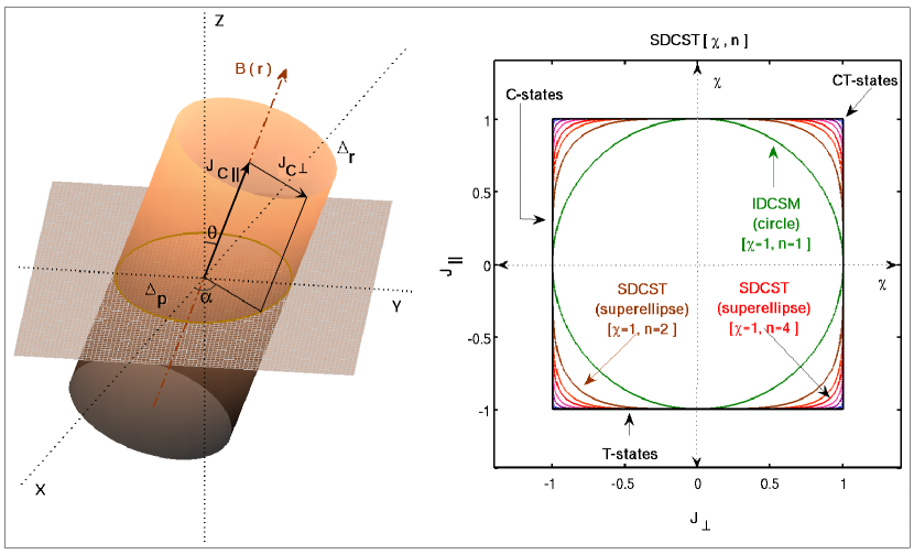
Figure 4.1: Left: The critical current restriction is represented by a cylindrical region $\Delta_{\textbf{r}}$ around the local magnetic field axis (length $2J_{c\parallel}$ and diameter $2J_{c\perp}$), $\Delta_{p}$ is the projection on the plane (x,y), $\alpha$ is the angle between the in-plane field projection and the x-axis, and $\theta$ is the angle between the field and the $z$ axis. Right: Geometrical representation of some of the material-law models depicted into the SDCST. The width and height of the region is controlled by the anisotropy parameter $\chi^{2}=J_{c\parallel}^{2}/J_{c\perp}^{2}$, and a smoothing index $n$.

In this chapter, and corresponding to the material laws depicted in the right side of figure 4.1, we will show that the variational statement may be used to predict the magnetic response of type-II superconductors with 3D anisotropy. In a first part, we will give the details related to the mathematical statement of the general critical state in a three dimensional slab geometry, i.e., both in-plane and perpendicular magnetic field components are applied to an infinite slab and varied in a given fashion. Then, the second and third part are devoted to apply the theory and predict the magnetic structure for the limiting cases, i.e., on one hand, the isotropic model ($\chi^{2}=1,n=1$) and on the other hand, the infinite width-band model ($\chi^{2}\rightarrow\infty$) or model of T-states. Subchapter 4.4 is devoted to explore the set of effects associated to the DCSM hypothesis ($\chi^{2}\geq 1,n\rightarrow\infty$). A wide range of applied fields will be considered, and our results compared to those with possible analytical approaches. Finally, as we are highly interested in knowing and understanding the role played by the physical mechanisms of flux depinning and flux cutting, the last part addresses different physical scenarios by means of different smooth double critical state models paying special attention to the influence of the smoothing index $n$ and the widthband $\chi$. In any case, smooth models have to be considered as related to a number of experiments that one could not explain within piecewise continuous models [5, 6, 7, 8, 9, 10] or the previous ones. In addition, appendix 1 explores the concept of critical angle gradient in 3D systems, as an alternative model to deal with anisotropic systems in the slab symmetry.

  4.1 3D variational statement in slab geometry

In this subchapter, we derive a specific variational formulation in superconducting slabs for eventual 3D local field configurations (figure 4.1), i.e., both in plane and transverse local magnetic field components emerge as derived effects of the flux depinning and flux cutting mechanisms. To be specific, we will consider an infinite slab, cooled under the assumption of an initial state defined by a uniform vortex lattice perpendicular to the external surfaces (i.e., a constant magnetic field $H_{z0}$), and then subjected to a certain process for the applied parallel field (i.e., $[H_{x0}(t),H_{y0}(t)]$) as is indicated in Fig. 4.2.

Recalling the symmetry properties of the electromagnetic quantities, one can describe the problem as a stack of current layers parallel to the sample’s surface, in such manner that the slab occupies the space $|z|\leq a$. Thus, it suffices to discretize the upper half, i.e.: $0\leq z_{i}\leq a$ as symmetry (or antisymmetry) conditions may be applied, and the position independence for a given value of $z_{i}$ ensures a divergenceless ${\bf J}$. Notice also that, within this approximation, one has to include two components of ${\bf J}$ within each layer, i.e.: $[J_{x}(z_{i}),J_{y}(z_{i})]$. At this point it would be worth mentioning that in order to simplify the mathematical statements we shall normalize the electrodynamic quantities by defining $\textbf{h}\equiv\textbf{H}/J_{c\perp}a$, $\textbf{j}\equiv\textbf{J}/J_{c\perp}$, and $\texttt{z}\equiv z/a$. Recall that one may assume the numerical value $J_{c\perp}$ as known a priori or obtained from experiment. In turn, our problem will be described in terms of $N_{s}$ discretized layers of equal thickness $\delta$ ($z_{i}=\delta\,i\;,\;\delta\equiv a/N_{s}$), each one characterized by a current density function $\textbf{j}(z_{i})=\textbf{j}_{x}(z_{i})+\textbf{j}_{y}(z_{i})$ distributed along $|z_{i}|\leq N_{i}a/N_{s}$. Eventually, for each layer, the unknown variables entering the minimization procedure may be defined accordingly to sheet currents, $I_{i,l+1}^{x}\equiv\delta j_{x}(z_{i},t=l+1)$ and $I_{i,l+1}^{y}\equiv\delta j_{y}(z_{i},t=l+1)$.

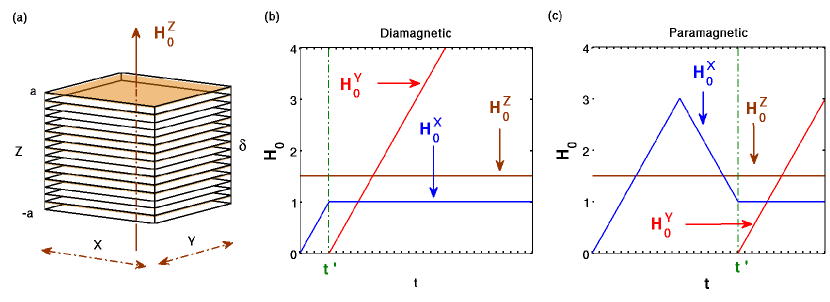
Figure 4.2: One the one hand, we show a pictorial illustration of the slab geometry with a perpendicular magnetic component $H_{z0}$ [sketch (a)]. On the other hand, schematics of the time dependence of the applied magnetic fields in the diamagnetic and paramagnetic configurations are depicted [sketches (b) and (c), respectively]

Then, a straightforward application of Ampère’s law allows to express the penetrating magnetic field along the $x-axis$ as the sums over the layers:

$$h_{x}(z_{i})\equiv h_{i}^{x}=-\sum_{j>i}I_{j}^{y}-I_{i}^{y}/2\,.$$ (4.1)

Similarly, the local profiles for the longitudinal magnetic field component $h_{y}(z_{i})$ can be evaluated from,

$$h_{y}(z_{i})\equiv h_{i}^{y}=\sum_{j>i}I_{j}^{x}+I_{i}^{x}/2\,.$$ (4.2)

Following the concept introduced in the previous chapter [see Eq. (3.3)], the following form of the objective function over the current sheets arises

$${\cal F}[I_{l+1}]= \leavevmode\nobreak\ \frac{1}{2}\sum_{i,j}I_{i,l+1}^{x}{\rm M}_{ij}^{x}I_{j,l+1}^{x}-\sum_{i,j}{\rm I}_{i,l}^{x}{\rm M}_{ij}^{x}I_{j,l+1}^{x}$$ (4.3)

$$+\frac{1}{2}\sum_{i,j}I_{i,l+1}^{y}{\rm M}_{ij}^{y}I_{j,l+1}^{y}-\sum_{i,j}{\rm I}_{i,l}^{y}{\rm M}_{ij}^{y}I_{j,l+1}^{y}$$

$$-\sum_{i}I_{i,l+1}^{y}(i-1/2)({\rm h}_{0,l+1}^{x}-{\rm h}_{0,l}^{x})$$

$$+\sum_{i}I_{i,l+1}^{x}(i-1/2)({\rm h}_{0,l+1}^{y}-{\rm h}_{0,l}^{y})\,.$$

In an effort to provide an easier understanding of the above functional, we stress that only the physical quantities playing the role of unknowns are shown in italics. Then, we may straightforwardly identify the quadratic and linear groups for the minimization procedure. In detail, the sheet currents $I_{l+1}^{x}$ and $I_{l+1}^{y}$ represent the unknown variables to be minimized as a given initial state $[{\rm I}_{l}^{x},{\rm I}_{l}^{y}]$ is connected by the steady processes $\Delta{\rm h}_{0}^{x}={\rm h}_{0,l+1}^{x}-{\rm h}_{0,l}^{x}$ and $\Delta{\rm h}_{0}^{y}={\rm h}_{0,l+1}^{y}-{\rm h}_{0,l}^{y}$, and their mutual inductance matrices ${\rm M}_{ij}^{x}$ and ${\rm M}_{ij}^{y}$. It is to be noticed that the index $l$ is introduced to indicate time discretization, i.e., $I_{i}(l+\delta t)-I_{i}(t)\equiv I_{i,l+1}-I_{i,l}$. When this index is omitted, it will be meant that the element is time independent, i.e., it is valid for any step $l$ and calculated as an external input for the objective function (see Figs. 3.1 & 3.2).

On the other hand, recall that the inductance matrices are directly linked to the design of a grid representing the location of variables into the superconducting volume. Thus, in the slab symmetry the circuits are just layers made up of straight lines along the $x$ and $y$ axis, and $\{I_{i}^{x},I_{i}^{y},\forall i\in\Omega\}$ is a compact notation for the whole set. Then, for our discretized array of layers the reader can check that a straightforward substitution of the squared components of the magnetic field entering the expression in Eq. (2.11) in terms of Eqs. (4.1) & (4.2), leads to the following formulas for the mutual inductance coupling elements:

$${\rm M}_{ij}^{x}={\rm M}_{ij}^{y} \equiv 1+2\left[{\rm min}\left\{i,j\right\}\right]\quad\forall\;i\neq j$$

$${\rm M}_{ii}^{x}={\rm M}_{ii}^{y} \equiv 2\left(\frac{1}{4}+i-1\right)$$ (4.4)

Notice that inductive coupling only occurs between $x$ and $y$ layers separately, and the corresponding coefficients are identical.

Finally, we stress that minimization has to be performed under a prescribed material law $\textbf{J}\in\Delta_{\textbf{r}}$ (i.e., some of the geometrical regions depicted in Figure 4.1), and ${\cal F}$ turns a new minimization functional for each different time step $(l=1,2,...)$. Specifically, the three dimensionality of the local magnetic field vector is controlled by the threshold values for the physical mechanisms responsible of the depinning and cutting of the vortices, i.e., the critical values $J_{c\parallel}$ and $J_{c\perp}$. Thus, in order to understand the three dimensionality of the vector J one has to consider the polar decomposition

$${\bf J}_{i}={\bf J}_{i}^{\parallel}+{\bf J}_{i}^{\perp\alpha}+{\bf J}_{i}^{\perp{\theta}}\,,$$ (4.5)

with the parallel, azimuth and polar components of ${\bf J}_{i}$ defined in terms of the magnetic field direction $\textbf{\^{H}}_{i}$. After some simple algebraic operations in a Cartesian coordinate system, the following expressions are obtained for such components:

1. The current component parallel to $\textbf{\^{h}}_{i}$ or so-called cutting current component $I_{i}^{\parallel}$:

   $$I_{i}^{\parallel}=\frac{h_{i}^{x}I_{i}^{x}+h_{i}^{y}I_{i}^{y}}{\left[(h_{i}^{x})^{2}+(h_{i}^{y})^{2}+(h_{i}^{z})^{2}\right]^{1/2}}\,.$$ (4.6)

2. The component of ${\bf I}$ perpendicular to the plane defined by the vectors ẑ and ĥ or so-called azimuthal current component

   $$I_{i}^{\perp\alpha}=\frac{-h_{i}^{y}I_{i}^{x}+h_{i}^{x}I_{i}^{y}}{\left[(h_{i}^{x})^{2}+(h_{i}^{y})^{2}\right]^{1/2}}\,.$$ (4.7)

3. The component of ${\bf I}$ perpendicular to ĥ and contained in the plane defined by the vectors ẑ and ĥ or so-called polar current component $I_{\perp\theta}$:

   $$I_{i}^{\perp\theta}=\frac{h_{i}^{z}(h_{i}^{x}I_{i}^{x}+h_{i}^{y}I_{i}^{y})}{\left\{\left[(h_{i}^{x})^{2}+(h_{i}^{y})^{2}+(h_{i}^{z})^{2}\right]\leavevmode\nobreak\ \left[(h_{i}^{x})^{2}+(h_{i}^{y})^{2}\right]\right\}^{1/2}}\,.$$ (4.8)

Thus, as an example, within the framework of the DCSM hypothesis one has to invoke the conditions

$$\left(1-(h_{i}^{x})^{2}\right)(I_{i}^{x})^{2}+\left(1-(h_{i}^{y})^{2}\right)(I_{i}^{y})^{2}-2h_{i}^{x}h_{i}^{y}I_{i}^{x}I_{i}^{y}\leq{\rm I}_{c\perp}^{2}\,,$$ (4.9)

and

$$(h_{i}^{x}I_{i}^{x})^{2}+(h_{i}^{y}I_{i}^{y})^{2}+2h_{i}^{x}h_{i}^{y}I_{i}^{x}I_{i}^{y}\leq{\rm I}_{c\parallel}^{2}\,.$$ (4.10)

In summary, the objective function is constrained by the group of functions defined by Eqs. (4.9) & (4.10), and their minimization provides the magnetic response of the superconductor by means a collection of discretized current elements for the planar sheets of current density $[j_{i}^{x},j_{i}^{y}]$ at the time steps $l+1=1,2,3,...$.

  4.2 Isotropic predictions in “3D” configurations

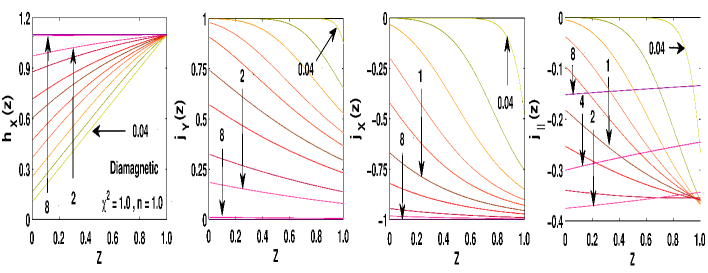
Figure 4.3: In the diamagnetic configuration and the isotropic model ($\chi^{2}=1$,$n=1$), we show the profiles for the local magnetic field component $h_{x}[z,h_{y}(a)]$ and their corresponding current-density profiles $j_{y}[z,h_{y}(a)]$, starting from a first-time step defined by $h_{x}(a)=1.1$ and $h_{z0}=1.5$. The current component $j_{x}[z,h_{y}(a)]$ and the cutting component $j_{\parallel}[z,h_{y}(a)]$ are also shown. The curves are labeled according to the component of longitudinal magnetic field at the slab surface, and correspond to the values $h_{y}(a)=0.040,0.2,0.4,0.6,0.8,1.0,1.2,1.6,2.0,4.0,$ and $8.0$.

Below, we show the theoretical predictions for the region or material law defined by the region $(\chi^{2}=1,n=1)$ or isotropic model (see Fig. 4.1), along the magnetization processes indicated in Figure 4.2.

Starting from a fully penetrated state with a magnetic field applied perpendicular to the slab surfaces ($h_{z0}$), i.e., a lattice of parallel vortices is assumed to nucleate parallel to the $z$ axis within the sample, one configures either a diamagnetic or a paramagnetic critical state by sweeping an applied parallel component $h_{x0}$ (thus inducing $j_{y}$). For example, if in a first temporal branch $(t<t^{\prime})$ the material is subjected to an increasing magnetic field $h_{x}$ by means of $\Delta h_{x}(a)$, time path steps are characterized by tilted flux lines which penetrate the specimen until an equilibrium distribution is achieved (diamagnetic). Then, if the external magnetic field is subsequently lowered, thereby reducing the retaining magnetic pressure, flux lines migrate out of the sample until the equilibrium is restored (paramagnetic).

Eventually, at $t=t^{\prime}$ an increasing ramp in the other longitudinal field component $h_{y0}$ is switched on and thus, an electric field $E_{x}$ arises at a surface layer of the superconductor which produces a current density $j_{x}$ that will screen the excitation. Then, owing the restrictions on the current density vector ${\bf j}$ introduced by the material law, the local component $j_{y}$ is affected and the corresponding local magnetic field $h_{x}(z)$ is pushed towards the center of the sample in the diamagnetic case (see Figure. 4.3) or towards the external surface in the paramagnetic one (see Figure. 4.4).

In detail, figures 4.3 & 4.4 show how the local component $h_{x}(0)$ increases (diamagnetic case) or it reduces (paramagnetic case) until the specimen is fully penetrated to satisfy the condition $h_{x}(z)=h_{x}(a)\;\forall\leavevmode\nobreak\ z$, i.e., $j_{y}(z)\rightarrow 0$ as $h_{y}$ increases. As a consequence, no sign reversal in the induced currents is predicted. Two important features of this model are to be remarked.

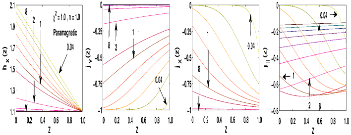
Figure 4.4: Same as figure 4.3, but in the paramagnetic configuration illustrated in figure 4.2. Here, the curves are labeled according to the values $h_{y}(a)=0.040,0.2,0.4,0.6,0.8,1.0,1.2,2.0,3.0,4.0,5.0,6.0,7.0,$ and $8.0$.

On the one hand, it has to be recalled that by the symmetry conditions invoked before, we may assert that, for long loops, the contribution coming from the U turn at the far ends, exactly equals the contribution of the long sides. This may be shown starting from the condition $\nabla\cdot\textbf{J}=0$ (no sources) that allows us to consider the current-density distribution as a collection of loops and ensures the equality of the integrals over $zj_{x}$ and $zj_{y}$. Thus, the magnetic moment components per unit area may be obtained by numerical integration of the current density along the slab thickness, i.e.,

$$\textbf{M}=\int_{-a}^{a}\textbf{z}\times\textbf{j}dz\,.$$ (4.11)

Then, the saturation of the current components $j_{x}(z)$ and $j_{y}(z)$, indicates that the isotropic hypothesis ($j_{c}=j_{c\parallel}=j_{c\perp}$ i.e., $\chi^{2}=1,n=1$) is providing a straightforward explanation of the observed magnetization collapse [11]. Furthermore, by comparison between the Figs. 4.3 & 4.4 with their corresponding magnetization curves (see curves in green in Fig. 4.5), we also noticed that the magnetization collapse is obtained simultaneous to the monotonic reduction of the cutting current density or $j_{\parallel}$.

On the other hand, another related phenomenon, the so-called paramagnetic peak effect of the magnetic moment can not be foreseen by the isotropic material law. As a consequence, more sophisticated models have to be either invoked and revalidated by the study of the components of cutting and depinning for the current density. It has to be mentioned, that in previous works far away of the DCSM hypothesis, this observation was explored in terms of the so-called two velocity electrodynamic model as a crude approximation for the real dynamics in a flux line lattice (see details in Ref. [12])

  4.3 T-states in “3D” configurations

In this section we continue the previous discussion, but now assuming a region with an infinite band-width $(\chi\rightarrow\infty)$ or so called model for T-states. Recalling that the magnetic field h is measured in units of the physically relevant penetration field $J_{c\perp}a$ then, numerical experiments with $h_{z0}=0.1$, $h_{z0}=1.5$, and $h_{z0}=10$ will cover the range of interest.

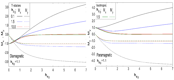
Figure 4.5: The magnetic moment $M_{x}$ (solid lines) and $M_{y}$ (dashed lines) per unit area as a function of the applied magnetic field component $h_{y0}$ in the diamagnetic (left pane) and paramagnetic (right pane) initial configurations of Fig. 4.2. Several cases are shown accordingly to the field intensities: $h_{x0}=1.1$ together with $h_{z0}=0.1$ (black), $h_{z0}=1.5$ (blue), and $h_{z0}=10.0$ (red), for the T-states model. Also, the corresponding curve for $h_{x0}=1.1$ and $h_{z0}=1.5$ for the isotropic model (green) are shown. Units are $j_{c\bot}a$ for $h$ and $j_{c\bot}a^{2}$ for $M$.

In figure 4.5 we display our results for the magnetic moment components per unit area under the experimental conditions depicted in figure 4.2. The plots indicate the following features:

1. In general, a saturation is reached for $M_{y}(h_{y0})$, as compared to the eventual linear increase of $M_{x}(h_{y0})$ for the highest values of $h_{y0}$.

2. The higher $h_{z0}$, the sooner the saturation is reached.

3. Increasing $h_{z0}$ rapidly diminishes the slope of $M_{x}(h_{y0})$.

4. In the paramagnetic case, a minimum is observed (more evidently for $M_{x}$, and more visible for $h_{z0}=1.5$), that is smoothed either for the higher or lower values of this field component.

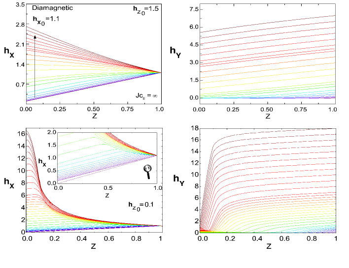
Figure 4.6: Magnetic field components $h_{x}(z)$ (left) and $h_{y}(z)$ (right) corresponding to the current-density profiles for the T-state limit in the diamagnetic configuration with $h_{z0}=1.5$ (top) and $h_{z0}=0.1$ (bottom) respectively.

Here, we want to call readers’ attention on the fact that our results for moderate perpendicular fields ($h_{z0}=1.5$ and $h_{z0}=10$) are in perfect agreement with the differential equation approach provided by Brandt and Mikitik in Ref. [13] (for more details see Ref. [2]). For these cases, the underlying flux penetration profiles fully coincide with our calculations. However, in Ref. [13] the low field region was uncovered. Thus, here we will show the exotic behavior of the field and current-density profiles for the low field regime (e.g., $h_{z0}=0.1$) in comparison with the local electromagnetic behavior for moderate fields (e.g., $h_{z0}=1.5$).

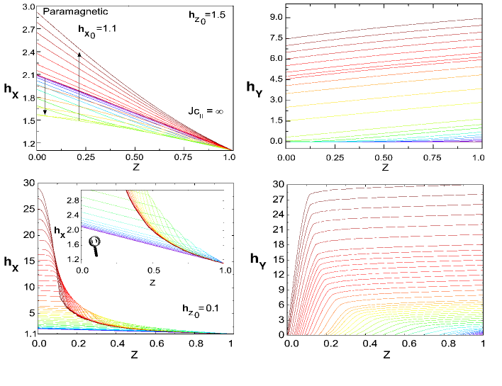
Figure 4.7: Same as Fig. 4.6 but for the paramagnetic configuration

Figures 4.6 & 4.7 respectively display the behavior of the in-plane magnetic field components [$h_{x}(z)$,$h_{y}(z)$] in the diamagnetic and paramagnetic cases. On the one hand, in the diamagnetic case we notice that for moderate fields, the local magnetic field $h_{x}(z)$ is monotonically pushed towards the center of the sample with a nearly homogeneous distribution of the cutting current component $j_{\parallel}$ (see figure 4.8). In an analogous manner, for the paramagnetic case the dynamics of the local component $h_{x}(z)$ is also related to the dynamics of the cutting current component. Thus, in a first stage the array of vortices closer to the center of the sample shows a decrease of the local component $h_{x}(z)$ until the full penetration state for the applied magnetic field $h_{y}(z)$ is achieved. Then, the cutting condition $j_{\parallel}\neq 0$ is warranted for the whole sample. Interestingly, once the center of the sample reaches the cutting condition a fast change of sign in the slope of $j_{\parallel}$ is envisaged which straightforwardly corresponds to the change of sign in the slope of the magnetic moment $M_{x}$ or peak effect. In turn, it leads to a second stage which is mainly characterized by an array of vortices with a monotone increase of the components $h_{y}(z)$ and $h_{x}(z)$ under the boundary condition for the initial state (e.g., in our cases we have assumed $h_{x}(a)=1.1$ for t=t’, see also Fig. 4.2).

On the other hand, it is to be noticed that the effects induced by the consideration of an unbounded cutting component are rather less simple for the low field regime (e.g., $h_{z0}=0.1$). Indeed, a steep variation of $h_{y}$ occurs for the inner region of the sample, corresponding to large values of $j_{\parallel}$ essentially dominated by $j_{x}$. On the contrary, $h_{x}$ displays a small slope, which relates to the condition $j_{\perp}=1$ (essentially, $j_{\perp}\approx j_{y}$ in the inner region).

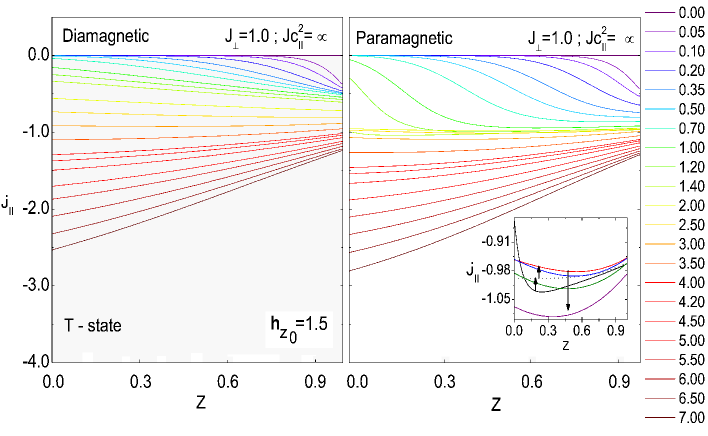
Figure 4.8: Profiles of the parallel current component $j_{\parallel}$ for the T-state hypothesis “$J_{c\parallel}\to\infty$ and $J_{c\perp}=1.0$”. The curves are labeled according to the applied field $h_{y0}$ (at right), assuming $h_{z0}=1.5$. The diamagnetic (left pane) and paramagnetic (right pane) cases are shown. In the paramagnetic case, the profiles of $J_{\parallel}$ for $h_{y0}=1.35,\,1.7,\,2.0,\,2.3,\,2.6,\,3.0$ are shown as an inset, and correspond to the sign change in the slope of the magnetic moment $M_{x}$ (see figure 4.5).

More into detail, Fig. 4.9 displays the behavior of the projection of the current density onto the direction of the magnetic field ($j_{\parallel}$) under the ansatz of a T-state structure for $h_{z0}=0.1$. It is apparent that the full penetration of the T-state perturbation requires a high field component ($h_{y0}\approx 18$ and $h_{y0}\approx 30$ for the diamagnetic and paramagnetic cases respectively), and a very high ratio $J_{\parallel}/J_{c\perp}\equiv j_{\parallel}$ ($\approx 180$ for the diamagnetic case and $\approx 340$ for the paramagnetic one). Notice that until these values are reached, one has $J_{\parallel}=0,J_{\perp}=1$ for the inner part of the sample, and a certain distribution $J_{\parallel}(z)$ for the outer region. We also recall a somehow complex structure with one or two minima in between the surface of the sample and the point reached by the perturbation. Interestingly, when $h_{y0}$ grows, the minimum becomes very flat, corresponding to a nearly constant value of $j_{\parallel}$. From the physical point of view, the minimum basically represents the region where ${\bf h}$ rotates so as to accommodate the penetration profile ${\bf h}(z)$ to the previous state of magnetization $(h_{x},0,h_{z0})$. From the point of view of Faraday’s law, this takes place as quickly as possible so as to minimize flux variations.

Finally, we want to call readers’ attention on two derived facts from this model. On the one hand, is to be noted that within the T-states model the magnetization collapse does not take place at least for perpendicular fields lower than $h_{z0}=10$. Indeed, a tiny slope on the magnetization moment curve is still present (see Fig. 4.5). On the other hand, as consequence of the non constrained cutting component, there is no restriction on the longitudinal component of the current density that increases arbitrarily towards the center of the sample (see Figs. 4.6 & 4.7). Thus, strictly speaking, this model can not be consider as physically admissible although some of the experimental evidences may be reproduced.

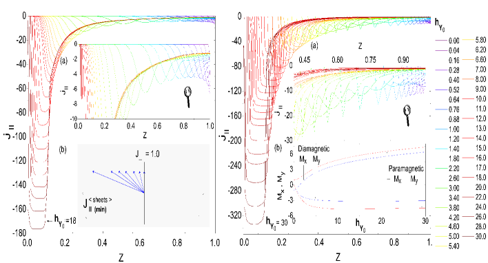
Figure 4.9: Profiles of the component $j_{\parallel}$ for the limit $J_{c_{\parallel}}\to\infty$ (T-state) with $h_{z0}=0.1$. In all cases the perpendicular current profiles satisfy $J_{\perp}=J_{c\perp}=1.0$. The diamagnetic (left) and paramagnetic (right) cases are shown. Left: inset (a) shows a zoom of $j_{{||}}$ for the first profiles of $h_{y_{0}}$. Inset (b) schematically shows the evolution of the vector $\bf J$ as function of its parallel and perpendicular components. Bottom: inset (a) shows a zoom of $j_{{||}}$ for the first profiles of increasing $h_{y0}$. Inset (b) shows the magnetic moment components ($M_{x}$, $M_{y}$) per unit area as a function of $h_{y0}$.

  4.4 CT-states in “3D” configurations

Below, we show the theoretical predictions derived by choosing a rectangular region for the material law $\Delta_{r}$ with a finite bandwidth $\chi$ or so-called DCSM (i.e., $\chi\geq 1$ and $n\rightarrow\infty$ within our SDCST). In order to keep the previous sequence of results and the underlying ideas, the same numerical experiments depicted in Fig. 4.2 will be analyzed.

Before going into detail, let us recall that the cases analyzed in the previous two sections directly correspond to the lower and higher limits of the double critical state approach, and in consequence, any material law displayed between them will be characterized by intermediate profiles for the electromagnetic quantities (more details in Refs. [2, 3]). Thus, we can summarize the rich phenomenology encountered by means a thorough analysis of the magnetic moment curves $M_{x}(h_{y0})$ and $M_{y}(h_{y0})$, and the local profiles for the cutting current component $j_{\parallel}(z)$.

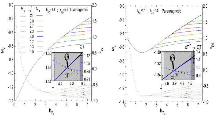
Figure 4.10: Magnetic moment curves per unit area ($M_{x},M_{y}$) as a function of the applied field $h_{y0}$ for the experimental configurations displayed in Fig. 4.2. Shown are the diamagnetic (left) and paramagnetic (right) cases for $h_{x0}=1.1$ and the moderate perpendicular field $h_{z0}=1.5$. The T-state curves ($j_{c\parallel}\gg 1$) are shown for comparison with the DCSM-cases: $j_{c_{||}}^{2}=$3.0, 2.7, 2.3, 2.0, 1,7, 1.3, 1.0. The insets show the particular case $j_{c_{||}}^{2}=2.0$ in the region where the transition T$\rightarrow$CT is visible.

Firstly, we show the corrections to $M_{x}$ and $M_{y}$ both for the diamagnetic and paramagnetic cases either at a moderate perpendicular field (Figure 4.10) or at a low perpendicular field (Figure 4.11), when the DCSM region corresponds to the aspect ratio values $\chi^{2}=1.0,1.3,1.7,2.0,2.3,2.7$ and $3.0$.

On the one hand, for a moderate perpendicular field (e.g., $h_{z0}=1.5$), it is noticeable that the limitation in $j_{c\parallel}$ produces a corner in the magnetic moment dependencies $M_{x,y}(H_{y0})$, which establishes the departure from the master curve defined by the T-state model. The corner in $M_{x}$ and $M_{y}$ appears at some characteristic field $h_{y0}^{*}$ that increases with $\chi$, eventually disappearing within the region of interest. Thus, the higher value of $h_{y0}$ for which the corner can not be observed ($h_{y0}\approx 3$ in the conditions depicted into the plots of Fig. 4.10), defines the acting threshold of the T-state model. The fine structure of the corner is shown in the insets of Fig. 4.10. Notice that, indeed, the deviation from the master curve takes place in two steps, being the second one that really defines the corner.

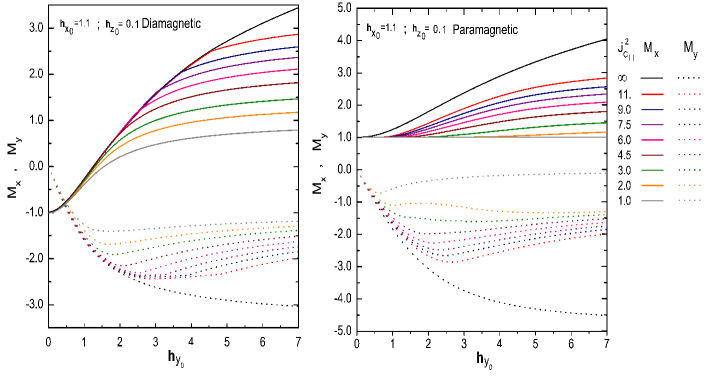
Figure 4.11: Same as figure 4.10, but in the lower perpendicular field regime $h_{z0}=0.1$. Here, the following DCSM-cases: $J_{c_{\parallel}}^{2}=$ 11.0, 9.0, 7.5, 6.0, 4.5, 3.0, 2.0, and 1.0, are shown.

On the other hand, for a low perpendicular field (e.g., $h_{z0}=0.1$), the general trends in the CT-state corrections do not very much differ from those at moderate field values. However, some distinctive features are worth to be mentioned for the $M_{x,y}(H_{y0})$ curves (Figure 4.11). To start with, we recall that the corner structure that defines the separation of the CT-curves from the master T-state behavior is different. Thus, as one can notice in Fig. 4.11, it is only for the higher values of the parameter $\chi^{2}$ that the separations take place abruptly. In particular, a smooth variation occurs for $\chi^{2}<6$ in all cases. Also noticeable is the change in the behavior of the initial part of the $M_{x}(h_{y0})$ curves for the paramagnetic case. Recall that the minimum observed for the moderate field patterns ($h_{z0}=1.5$) has now disappeared (this can be already detected for the T-states). Significantly, one can observe that by decreasing $\chi^{2}$, $M_{x}$ develops a nearly flat region at the low values of $h_{y0}$. Physically, this means that the initial $h_{x}(z)$ profile is basically unchanged. For the lowest values of $\chi^{2}$ this can take place over a noticeable range of applied fields $h_{y0}$ [2].

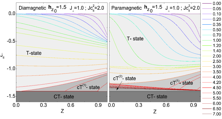
Figure 4.12: Profiles of the parallel currents $j_{\parallel}$ for the rectangular region hypothesis or DCSM with $J_{c\parallel}^{2}=2$ and $J_{\perp}=J_{c\perp}=1.0$. The curves are labeled according to the applied field $h_{y0}$ (at right), assuming $h_{z0}=1.5$. The diamagnetic (left) and paramagnetic (right) cases are shown.

Secondly, with the aim of providing a fair understanding on how the T-states break down for the 3D configurations studied in this chapter, in Figure 4.12 we have plotted the local profiles of $j_{\parallel}(z)$ for a moderate perpendicular field $h_{z0}=1.5$ while the external magnetic field $h_{y0}$ is increased. The left pane shows the process of saturation in which $j_{\parallel}$ reaches the value $j_{c\parallel}$ for the diamagnetic initial condition. Analogously, the right pane shows their corresponding behavior but for the paramagnetic initial condition. To allow a physical interpretation of these profiles, we have introduced the following notation: $cT$ denotes that $j_{\parallel}$ has reached the limit $j_{c\parallel}$ only partially within the sample, while $CT$ means that $j_{\parallel}$ equals $j_{c\parallel}$ for the whole range $0\leq z\leq a$. For the partial penetration cT-states, we additionally distinguish between the so-called cT⁽¹⁾ and cT⁽²⁾ phases. As one can see in the plot, cT⁽¹⁾ means that $j_{\parallel}$ penetrates linearly from the surface until the limitation is reached somewhere within the sample. For the diamagnetic case, the profile stops at the actual value $j_{c\parallel}$. However, for the paramagnetic case, the structure is more complex. Thus, $j_{\parallel}$ penetrates linearly until a linear increase (towards the center) curve is reached. This structure is followed until the contact between both lines reaches the surface. Then, the so-called cT⁽²⁾ region appears. The cutting current component $j_{\parallel}$ has reached the threshold value $j_{c\parallel}$ at the surface, and the whole $j_{\parallel}$ curve “pivots” around this point until the full CT-state is reached. We call the readers’ attention that the initial separations of the magnetic moment from the T-state master curves take place as soon as a cT-state is obtained. Further, the corners can be clearly assigned to the instant at which the full CT state appears.

Figure 4.13: Left pane: Profiles of the parallel ($J_{||}$) and perpendicular ($J_{\perp}$) current densities in the diamagnetic configuration at a low perpendicular field $h_{z0}=0.1$, for the rectangular region or DCSM law with $J_{c\parallel}^{2}=2.0$ and $J_{c_{\perp}}=1.0$. Central pane: Same as above, but the profiles for the paramagnetic configuration are shown. Right pane: Magnetic field components $h_{x}(z)$ (solid-lines) and $h_{y}(z)$ (dashed-lines) corresponding to the above mentioned paramagnetic configuration. For clarity, the $h_{y}(z)$ profile corresponding to $H_{y0}=1.40$ has been labeled accordingly. All the curves follow the same color scale convention corresponding to the values of the applied field $h_{y0}$. In left pane, inset (a) schematically shows the CT structure of the full penetration regime in the diamagnetic case. The CT-C structure behavior of ${\bf J}$ for the paramagnetic case is shown in the inset (b).

Also interesting are the peculiarities of the cutting and depinning components of the current density penetration profiles for low values of the perpendicular field $h_{z0}$. They can be observed in Figs. 4.13 & 4.14, which both reveal new physical mechanisms that do not appear for the moderate perpendicular field values. Once more, the first observation is that the appearance of the corner in the magnetic moment straightforwardly relates to the current density profiles. Thus, for the lower values of $\chi$ (no corner present), the profile $j_{\parallel}$ displays a rather simple structure, basically jumping from $0$ to $j_{c\parallel}$ at some point within the sample (Fig. 4.13). On the contrary, for the higher values of $\chi$ (those displaying a corner in $M_{xy}$) the evolution of the cutting profiles $j_{\parallel}(z)$ is much more complex (Fig. 4.14). Let us analyze these plots in more detail:

Firstly, Fig. 4.13 shows the cutting profiles $j_{\parallel}(z)$ both for the diamagnetic and paramagnetic cases with a DCSM region characterized by the parameter $\chi^{2}=2$. It is to be noticed that, in both cases, the step-like structure with $J_{\parallel}=0$ in the inner part and $J_{\parallel}=J_{c\parallel}$ in the periphery evolves until the full penetration state $J_{\parallel}=J_{c\parallel}\;,\;\forall\;z$ is reached. However, an outstanding fact is that in the paramagnetic case, for the first time along the exposition of this chapter we have met a set of conditions that produce an excursion of $j_{\perp}$, i.e., the customary condition $J_{\perp}=J_{c\perp}$ is violated during the process of increasing $h_{y0}$. To be specific, $J_{\perp}$ starts from the condition $J_{\perp}=J_{c\perp}$, given by the initial process in $h_{x0}$. Then, a basically linear decrease from some inner point towards the surface occurs, with an eventual reduction to a nearly null value at some regions within the sample (C-states are basically provoked). Further increase of $h_{y0}$ produces a new CT-state. This behavior is shown in a pictorial form within the insets of Fig. 4.13. Recall that the average current density sharply transits from a T-state ($J_{\perp}=J_{c\perp}\,,\,J_{\parallel}=0$) to the CT-state ($J_{\perp}=J_{c\perp}\,,\,J_{\parallel}=J_{c\parallel}$) for the diamagnetic case, while a T $\to$ C $\to$ CT evolution happens for the initial paramagnetic conditions. This behavior allows a physical interpretation in terms of the evolution of the magnetic field profiles. Thus, as stated before, the cases with small $\chi$ are characterized by a nearly frozen profile in $h_{x}$, as shown in right pane of Fig. 4.13. Then the structure of $h_{x}(z)$ and $h_{y}(z)$ is basically a cross between two straight lines, where the crossing point coincides with the minimum in $J_{\perp}(z)$. Thus, recalling the interpretation of the perpendicular component of the current density [Eqs. (4.7) & (4.8)], the minimum should be expected as $h_{x}^{2}+h_{y}^{2}$ has a very small variation around the crossing point of the two families of nearly parallel lines.

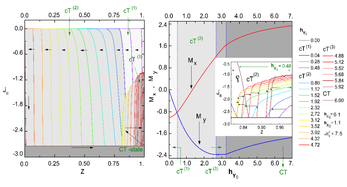
Figure 4.14: Left pane: Profiles of $j_{||}$ for the diamagnetic case within the rectangular DCSM with $\chi^{2}=7.5$ and $h_{z0}=0.1$. In all cases, one gets $J_{\perp}=J_{c\perp}=1.0$. Right pane: The corresponding magnetic moment components ($M_{x},M_{y}$) as a function of $h_{y0}$ are shown. The evolution from the initial full penetration T state to the final full penetration CT state takes place in three steps that are classified according to the structure along the sample width, by means the defined states: cT${}^{(1)}\equiv$ T-CT, cT${}^{(2)}\equiv$ T-CT-T, cT${}^{(3)}\equiv$ CT-T and eventually CT.

On the other hand, the details about the behavior of the cutting component $j_{\parallel}$ for the larger values of $\chi$ are presented in Fig. 4.14, that corresponds to the case $\chi^{2}=7.5$. Again, owing to the complexity of the structure, we introduce the notation cT⁽¹⁾, cT⁽²⁾ and cT⁽³⁾, that is explained below. Let us first recall that the corner appears when the partial penetration regime cT⁽³⁾ extinguishes and the full sample ($0<z<d/2$) satisfies the conditions $J_{\perp}=J_{c\perp}$ and $J_{\parallel}=J_{c\parallel}$ (i.e., CT). This property is clearly seen in the right pane of this figure. Thus, the cT⁽¹⁾ regime is characterized by a T region in the inner part of the sample ($J_{\perp}=J_{c\perp}$ and $J_{\parallel}=0$), that abruptly becomes CT at a point that progressively penetrates towards the center (T-CT structure). At a certain instant, the profile becomes T-CT-T because the outermost layers develop a subcritical $J_{\parallel}$. This is called cT⁽²⁾. Then, the central CT band grows towards both ends. In first instance, the inner T region becomes CT, giving a global CT-T structure, that we call cT⁽³⁾. In a final step, the surface T layer shrinks again to a null width and the full profile is a CT region. This instant establishes the appearance of the corner in the magnetization curves.

  4.5 Smooth critical states in “3D” configurations

As stated before, our smooth double critical state theory (SDCST) allows to specify almost any critical state law by means a simple mathematical statement that includes an index $n$ accounting for the smoothness of the $J_{\parallel}(J_{\perp})$ relation, and a certain bandwidth characterizing the magnetic anisotropy ratio $\chi=J_{c\parallel}/J_{c\perp}$ [see Eq. (2.19)]. The systematic consideration of the influence of these parameters is of remarkable importance as it allows a straightforward elucidation of the relation between diverse physical processes and the actual material law. Most of the experimental evidences reflecting accurate observations for the influence of the cutting effects onto the macroscopic measurements of magnetic moment for anisotropic superconducting samples, without transport current, may be summarized along two remarkable facts:

1. The occurrence of magnetization peaks which are mainly evident in paramagnetic configurations [5, 6, 7, 8, 9].

2. The collapse of the magnetization curves towards an ostensible isotropic response [8, 9, 10].

Nowadays, it is well known that the DCSM and its precursors (the T-state and Isotropic models) are not able to achieve a fair understanding of the above effects in a wide number of configurations, or at least these models do not handle environments with high magnetic fields [2]. This fact has lead to consider alternative models such as the two-velocity electrodynamic model [12], or the helical electrodynamic model [14], both lacking a solid physical basis for the mechanisms underlying the motion of vortices. In fact, being the threshold values for the cutting current component $(J_{c\parallel})$ and the depinning current component $(J_{c\perp})$ the main physical observables determining the magnetic anisotropy of a superconductor [15, 16, 17], within these models, other parameters have to be included ad-hoc.

Moreover, it is worth anticipating the following chapter, by mentioning that neither of the above mentioned models allow a correct explanation for the experimental remarks when the superconductor is also carrying a longitudinal transport current. Thus, the purpose of this section is vindicating the physical mechanisms of cutting and pinning, through a comprehensive study of the magnetic anisotropy of type II superconductors, by means the modification of the conventional DCSM which leads to the establishment of the SDCST. Such modifications can be justified as corrections to the simplifying ideas that flux depinning is only related to $J_{\perp}$ and the flux cutting is only related to $J_{\parallel}$. We emphasize that in a in a general scenario, one should consider the dependencies $J_{c\perp}=J_{c\perp}(J_{\parallel})$ and $J_{c\parallel}=J_{c\parallel}(J_{\perp})$ [2, 3, 13, 15, 16].

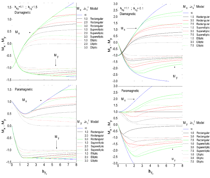
Figure 4.15: The magnetic moments $M_{x}$ and $M_{y}$ of the slab per unit area as a function of $h_{y_{0}}$ in the diamagnetic (top) and paramagnetic (bottom) cases with $h_{x0}=1.1$ and both for, a moderate perpendicular field $h_{z0}$=1.5 (left pane), and a low perpendicular field $h_{z0}=0.1$ (right pane). The “infinite band” or T-states model (blue solid lines), the DCSM or “rectangular regions” (other solid lines), the SDCST’s models with $n=4$ “superelliptical regions” (dashed-lines), and $n=1$ “elliptical regions” (dotted-lines), are shown for several values of the ratio $\chi^{2}\equiv j_{c\parallel}$ for a given $J_{c\perp}=1$.

Recalling that, mathematically, the effect of smoothing the corners for the rectangular DCSM region may be represented by a one-parameter family of superelliptical functions with the generic form given in Eq. (2.19), i.e.,

$$\left(\frac{J_{\parallel}}{J_{c\parallel}}\right)^{2n}+\left(\frac{J_{\perp}}{J_{c\perp}}\right)^{2n}\leq 1\,,$$

such kind of curves cover the whole range of interest just by allowing $n$ to take values over the positive integers. As the reader can easily verify for $\chi^{2}>1$, the index $n=1$ corresponds to the standard ellipse and $n\geq 4$ is basically a rectangle with faintly rounded corners (see Fig. 4.1).

In order to illustrate the effect of smoothing the material law $\Delta_{\textbf{r}}(\textbf{J}_{\parallel},\textbf{J}_{\perp})$ for different bandwidths $\chi$, below we will show the magnetization curves that are obtained for the diamagnetic and paramagnetic configurations considered before (Fig. 4.2). The main results of our analysis are depicted in Figs. 4.15 & 4.16.

Figure 4.15 shows the behavior of the magnetization curves $M_{x}$ and $M_{y}$ for an external perpendicular field of either moderate intensity $h_{z0}=1.5$ (left pane) or a lower intensity $h_{z0}=0.1$ (right pane). In order to simplify their interpretation, at this stage we will only compare the prediction for the smoothing index $n=4$ (superelliptic region) with the limiting cases $n=1$ (elliptic region) and $n\rightarrow\infty$ (a DCSM or rectangular region), under consideration of different bandwidths $\chi$.

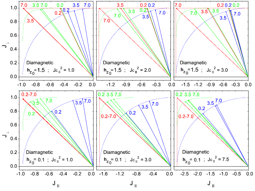
Figure 4.16: Current density vector J in the planar representation [$J_{\perp}$,$J_{\parallel}$] for three different material law models, corresponding to the following $\Delta_{\textbf{r}}$ regions: rectangular (red), superelliptical (green), and elliptical (blue). Here, the diamagnetic case for both a moderate field $h_{z0}=1.5$ and the lower field $h_{z}=0.1$ are shown. Several vectors for several values of the ratio $\chi=J_{c\parallel}/J_{c\perp}$ and the applied field $h_{y0}$ are shown and labeled on each arrow. The scales on the horizontal axes that have been re-sized for visual purposes.

Firstly, for the moderate perpendicular field region (left pane of Fig. 4.15), we observe that the overall effect of reducing the value of $\chi\equiv J_{c\parallel}/J_{c\perp}$ is the same for the three material laws or $\Delta_{\textbf{r}}$ regions. The smaller the value of $\chi$, the higher reduction respect to the T-state ($\chi\to\infty$) master curve for the magnetic moment components. On the other hand, as regards the particular details for each model, we recall: (i) as expected the smooth models lead to smooth variations, i.e.: the corner is not present, (ii) the breakdown of the T-state behavior occurs before (at higher values of $\chi$ or lower values of $h_{y0}$) for the smoother models. Strictly speaking, the concept of T-state is only valid for the rectangular region, but it is asymptotically generated as the superelliptic parameter $n$ grows. Finally, (iii) the isotropic CS limit, given by the circular region $n=1$ and $\chi=1$ produces the expected results [18]: $M_{x}$ collapses to zero, and $M_{y}$ develops a one dimensional critical state behavior.

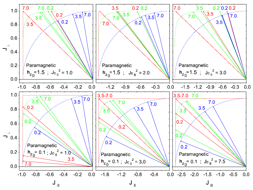
Figure 4.17: Same as Fig. 4.16, but here the $J$ vectors corresponds to the paramagnetic case.

Secondly, for the low perpendicular field region (right pane of Fig. 4.15, one can notice: (i) on the one hand, the rectangular and superelliptical models produce very similar results for the diamagnetic case, both for $M_{x}$ and for $M_{y}$, noticeably differing from the elliptical region predictions, that still show a practical collapse of $M_{x}$ and a saturation in $M_{y}$ as stated before. (ii) On the other hand, the paramagnetic case involves a higher complexity. Thus, we recall that the already mentioned feature of a “flat” behavior in $M_{x}$ for small values of $\chi$ within the rectangular region model, is no longer observed upon smoothing of the restriction region. On the contrary, the smooth models involve an initial negative slope and a minimum, resembling the behavior of $M_{x}$ for the rectangular model, but in moderate $h_{y0}$. As concerns $M_{y}$, important differences among the three models are also to be recalled.

In order to provide a physical interpretation of the behaviors reported in the above paragraphs for moderate and low perpendicular fields $h_{z0}$, a comparative plot of the current density vectors for each case is given in Figs. 4.16 & 4.17 respectively. For clarity, we restrict to the representation of the vector ${\bf J}$ at the surface of the sample ($z=a$) for a selected number of values of $h_{y0}$. Just at a first glance, one can relate the best coincidence in predicted magnetization to the more similar critical current density structures (superelliptical and rectangular regions for the diamagnetic case with $h_{z0}=0.1$). Recall that, in that case, the rectangular region produces a CT-state structure ($J_{\parallel}=J_{c\parallel}$ and $J_{\perp}=J_{c\perp}$) that is represented by a ${\bf J}$ vector, pinned in the corner. On the other hand, the vector ${\bf J}$ related to the superelliptic model does not pin at any point, because such a singular point does not exist. However, it is basically oriented in the same fashion and this relates to the good agreement in ${\bf M}$. We emphasize that the cases in which strong differences occur for the magnetic moment are also related to important changes in the behavior of ${\bf J}$. Thus, if one considers the paramagnetic case at small values of $h_{z0}$ and $h_{y0}$, the significant differences in magnetization relate to an opposite behavior in ${\bf J}$. Moreover, the rectangular model predicts a transition towards a C-state ($J_{\parallel}=J_{c\parallel}$ and $J_{\perp}\approx 0$), while the smooth versions produce a tendency towards the T-state (see left bottom panel of Fig. 4.17).

Appendix I Critical angle gradient in “3D” configurations

On the basis of minimum complexity, in this appendix the flux cutting criterion for 3D configurations will be revised under the assumption of a critical angle threshold instead of a superelliptical relation. Below let me present some results related to the concept of the critical angle gradient in 3D systems.

First recall that the limitation on $J_{\parallel}$ appears as related to the energy reduction by the cutting of neighboring flux lines when they are at an angle beyond some critical value [19, 20]. This concept has been largely exploited in the 2D slab geometry for fields applied parallel to the surface [4], and it is introduced by the local relation

$$\left|\frac{d\alpha}{dz}\right|=\left|\frac{J_{\parallel}}{H}\right|\leq K_{c}\,,$$ (4.12)

that establishes a critical angle gradient. Here, $\alpha$ stands for the angle between the flux lines and a given reference within the $XY$-plane (i.e.: an azimuthal angle). However, for the 3D cases under consideration, the relative misorientation between flux lines may also have a polar angle contribution, i.e.: ${\bf H}$ does not necessarily lie within the $XY$-plane or any other given plane.

As sketched in Fig. 2.1 (pag. 2.1), one has to introduce the angle $\gamma$ within the plane defined by the pair of flux lines under consideration. After some mathematical manipulations, it can be shown that, for the infinite slab geometry, with a three dimensional magnetic field one has

$$\frac{d\gamma}{dz}=\sqrt{\frac{J_{\parallel}^{2}}{H^{2}}+\frac{H_{z}^{2}J^{2}}{H^{4}}}=\frac{1}{H}\sqrt{J_{\parallel}^{2}+\frac{H_{z}^{2}}{H^{2}}\left(J_{\parallel}^{2}+J_{\perp}^{2}\right)}\,,$$ (4.13)

where the third component is also introduced. Actually, the above result is just a particular case of the relation

$$\nabla\times\left(B\hat{\bf B}\right)=\left[\left(\nabla B\right)\times\hat{\bf B}\right]+\left[B\;\left(\nabla\times\hat{\bf B}\right)\right]\equiv\left[{\bf J}_{\perp,1}\right]+\left[{\bf J}_{\perp,2}+{\bf J}_{\parallel}\right]\,,$$ (4.14)

showing that, in general, both ${\bf J}_{\parallel}$ and ${\bf J}_{\perp}$ can contribute to the spatial variation of the direction $\hat{\bf B}$.

Below, we display the effects of using the cutting limitation

$$\left|\frac{d\gamma}{dz}\right|\leq\kappa_{c}\,,$$ (4.15)

instead of assuming a constant value for the parallel critical current. Fig. 4.17 contains the main results. The calculations have been performed for the same diamagnetic and paramagnetic initial configurations displayed in Fig. 4.2.

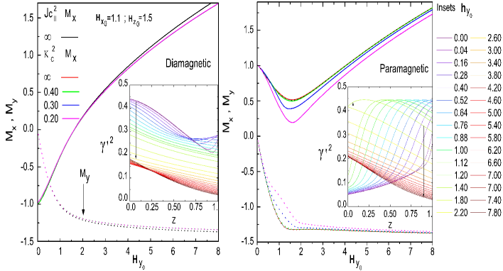
Figure 4.18: The magnetic moments per unit area $M_{x}$ (solid lines) and $M_{y}$ (dotted lines) of the slab as a function of $h_{y_{0}}$ for the critical angle gradient model [Eq.(4.15)]. The unrestricted case ($\kappa_{c}^{2}\to\infty$) is shown for comparison with several cases with a restricted angle gradient: $\kappa_{c}^{2}=$0.20, 0.30 and 0.40 (dimensionless units are defined by $\kappa_{c}\equiv K_{c}a$). Shown are the diamagnetic (left pane) an paramagnetic (right pane) cases for $h_{x_{0}}=1.1$ and $h_{z_{0}}$=1.5. The insets detail the evolution of the angle gradient profiles for $\kappa_{c}^{2}\to\infty$.

In general, one can see that the smaller values for the cutting threshold in whatever form produce the smaller magnetic moments (compare Figs. 4.10 & 4.11 with Fig. 4.18). However, some important differences are to be quoted. On the one hand, the critical angle criterion $|{\gamma}^{\prime}|\leq\kappa_{c}$ produces a smooth variation, by contrast to the corner structure induced by the critical current one $J_{\parallel}\leq J_{c\parallel}$. On the other hand, the effect of changing the value of $\kappa_{c}$ is much less noticeable, especially for the diamagnetic case, in which the full range of physically meaning values of $\kappa_{c}$ produce a negligible variation. Moreover, we call the readers’ attention that the above mentioned range for $\kappa_{c}$ is established by the application of Eq. (4.13) to the initial state of the sample. Thus, if one takes $J_{\parallel}=0,\,H_{z0}=1.5,\,H_{x0}=1.1$, the squared angle gradient takes the value ${\gamma}^{\prime 2}=0.19$ and one has to use $\kappa^{2}>0.19$ in order to be consistent with the initial critical state assumed.

Chapter 5 The Longitudinal Transport Problem

It is well known that various striking phenomena may occur when a type-II superconductor with intrinsic magnetic anisotropy is under the action of a transport current and a longitudinal magnetic field [2, 3, 7, 20, 33, 34, 25, 26, 35, 36, 21, 22, 23, 37, 38, 39, 40, 41, 42, 43, 44, 45, 24, 27, 28, 29, 17, 30, 31, 32, 46, 47]. In particular, a remarkable enhancement of the critical current density by means of its compression towards the center of the superconducting sample has been observed in a wide number of conventional and high temperature superconducting systems within a certain set of experimental conditions [20, 26, 25, 24, 27, 28, 29, 17, 30, 31, 32]. This property, together with other intriguing phenomena, such as the observation of paramagnetic moments, and outstandingly, the experimental observation of a counter intuitive phenomenon of negative resistance by the action of a parallel magnetic field, have been reported in the course of intense experimental and theoretical activities [7, 35, 36, 21, 22, 23, 37, 38, 39, 40, 41, 42, 43, 44, 45]. Most of these works were primarily concerned with the arrangement of the macroscopic current density ${\bf J}$ along the so-called nearly force free trajectories [48]. Recall that if ${\bf J}$ is nearly parallel to the magnetic induction ${\bf B}$, moderate or weak pinning forces are needed for avoiding the detrimental flux-flow losses related to the drift of flux tubes driven by the magnetostatic force (${\bf J}\times{\bf B}$ per unit volume). More specifically, negative voltages have been observed by different groups [35, 36, 21, 22, 23, 37, 38, 39, 21, 40, 41] when recording the current-voltage characteristics at specific locations on the surface of the sample (central region).

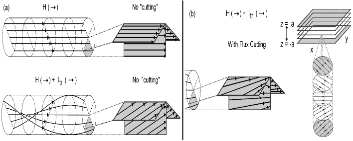
Figure 5.1: (a) Schematic representation of the helical model for the longitudinal transport problem in an infinite superconducting cylinder. An array of parallel helical fluxoids without flux cutting is assumed. (b) Pictorial illustration of the real situation where the flux cutting events appear. The cylindrical and slab symmetries are shown.

In a first approach, such resistive structure has been intuitively understood in terms of helical domains, closely connected to the force-free current parallel to the flux-lines [14, 21, 22, 23, 45, 29, 42]. The basic idea of this model relies in the fact that the averaged direction of the flux flow in a superconducting cylinder subjected to a longitudinal magnetic field and transport current, is the same as the direction of the Poynting’s vector $(\textbf{E}\times\textbf{H})$ onto the external surface, suggesting the occurrence of a continuous helical flux flow without flux cutting [see Fig. 5.1 (a)]. Also, in order to achieve a concordance with the experimental evidences [45, 29, 42], the resulting helical flux over the cylindrical surface must be subdivided in two domains for which the Poynting’s vector is directed in two concomitant directions: inwards (allowing the compressing of J towards the center of the specimen), and outwards (allowing the occurrence of surface regions with J flowing in counter direction to the flux of transport current). Nevertheless, despite the seeming simplicity of the helical model and its intuitive explanation for the increasing of the current density and the simultaneous occurrence of surface negative currents, the helical symmetry shown in Fig. 5.1(a) does not exist in any other symmetry different to the infinite cylinder, and furthermore, it does not include the flux cutting mechanism which causes many derived effects [see Fig. 5.1(b)]. Actually, regardless of the symmetry considered, there are some remarkable effects which can not be explained under this scenario. On the one hand, it has been stated that the direction of the helical structure and that of the magnetic field at the surface are really different [21, 22]. On the other hand, by increasing the magnetic field a continuous torsion of the helical domain should be expected, such that the vanishing of the negative current within a finite interval of the applied magnetic fields can not be conceived. Furthermore, it does neither explain the bounded increase of the transport current (i.e., the occurrence of a maximal peak on the longitudinal current density) as one raises the magnitude of the applied magnetic field. Finally, as a detail of fine structure, local paramagnetic domains cannot either be predicted within the above scenario. Therefore, a most accurate description of the diverse effects underlying to the longitudinal transport problem, have to include the physics behind the flux cutting mechanism.

Relying on our theoretical approach for the superconducting critical state problem in 3D magnetic field configurations and the aforementioned scenario, below we present an exhaustive analysis of the electrodynamic response for the so-called longitudinal transport problem of type-II superconductors in the slab geometry. Remarkable numerical and conceptual difficulties related to the implementation of the magnetic anisotropy and the relation between the flux-line cutting (crossing and recombination) and the flux-line depinning mechanisms, will be overcome by means simplified analytical models for extremal cases and the further comparison with the most general solution of the smooth double critical state theory (SDCST) for analogous material laws (subchapter 5.1). Then, supported by numerical simulations that cover an extensive set of experimental conditions, we put forward a much more complete physical scenario which is based upon a set of superelliptical material laws. Thus, subchapter 5.2 is devoted to show how the striking existence of negative flow domains, local and global paramagnetic structures, emergence of peak-like structures in both the critical current density and the longitudinal magnetic moment, as well as the compression of the transport current in type-II superconductors under parallel magnetic fields, are all predicted by our general critical state theory. In addition, we shall introduce some ideas that could be applied for the determination of the flux cutting threshold from local measurements of the current density flowing along specific layers of the superconducting sample, as correlated to the behavior of the magnetic moment components.

  5.1 Simplified analytical models and beyond

In this subchapter, we call the reader’s attention to the fact that two analytical approaches for the slab geometry in extreme situations may be found in the literature. The first one was introduced by Brandt and Mikitik in Ref. [13] for the regime of strong pinning with very weak longitudinal current conditions, i.e., $h_{z0}$ must be very high as compared to the in-plane applied field $h_{xy}(a)$ (then $J_{\parallel}\ll J_{c\perp}$). On the other hand, the opposite limit ($h_{z}\to 0$) was recently developed in our group (Ref. [33]). Thus, in a first stage let us show how the physical properties of the longitudinal transport problem may be understood within our simplified analytical model, and then we will move onto a general description of the problem in terms of the SDCST.

5.1.1 The simplest analytical model

First, recall that the Ampère’s law takes the following form for the infinite slab geometry considered in the previous chapter:

$$-\frac{dh_{y}}{dz}=j_{x}\quad;\quad\frac{dh_{x}}{dz}=j_{y}\,.$$ (5.1)

Also notice that, in the particular case $h_{z0}=0$ [i.e., $\theta=\pi/2$ in Fig. 4.1 (pag. 4.1)], the material law or region $\Delta_{p}$ becomes a rectangle with axis defined by the in-plane directions parallel and perpendicular to h. Thus, recalling the statements issued in chapter 4.1, one can show that such expressions may be transformed into the polar form

$$-h\frac{d\alpha}{dz}=j_{\parallel}^{\rm p}\quad;\quad\frac{dh}{dz}=j_{\perp}$$ (5.2)

with $h=\sqrt{h_{x}^{2}+h_{y}^{2}}$ the modulus of the magnetic field vector, and $\alpha={\rm atan}(h_{y}/h_{x})$ the angle between such vector and the $x$-axis.

Now, the thresholds of flux depinning and cutting imply the in-plane conditions

$$|j_{\parallel}^{\rm p}|\leq j_{c\parallel}^{\rm p}(\theta=\pi/2)=j_{c\parallel}\quad;\quad|j_{\perp}^{\rm p}|\leq 1\,.$$ (5.3)

Notice that, in general, Eq. (5.2) and the critical constraints defined in Eq. (5.3) would not straightforwardly lead to the solution of the problem. Thus, one should also use Faraday’s law, either by explicit introduction of the related electric fields (as in Refs. [15, 16]), or by our variational statement. However, as in this case $\theta=\pi/2$ and consequently $j_{c\parallel}^{\rm p}=j_{c\parallel}$, the resolution noticeably simplifies. In fact, for the considered situation, we will have a combination of the cases $j_{\parallel}^{\rm p}=\{0$ or $\pm j_{c\parallel}\}$, and $j_{\perp}^{\rm p}=\{0$ or $1\}$, and then integration of Eq. (5.2) is straightforward. For further mathematical ease, we will also consider $j_{c\parallel}$ and $j_{c\perp}$ to be field independent constants.

Following the notation introduced in chapter 4.4 we will refer to different zones within the sample that are basically related to macroscopic regions where well defined dissipation mechanisms occur. In brief, we will speak about T-zones, where only flux depinning (transport) occurs (${j}_{\parallel}=0\,,{j}_{\perp}=\pm 1$), C zones, where only flux cutting occurs (${j}_{\parallel}=\pm\chi\,,{j}_{\perp}=0$), CT zones where both transport and cutting occur (${j}_{\parallel}=\pm\chi\,,{j}_{\perp}=\pm 1$), and O-zones where neither flux transport nor cutting take place (${j}_{\parallel}=0\,,{j}_{\perp}=0$). Introducing the above set of possibilities in Eqs. (5.2) & (5.3) one gets the following cases for the incremental behavior of the magnetic field in polar components

$$dh=\left\{\begin{array}[]{rr}0\qquad\rm{(O,C)}&\\ \pm\,dz\;\;\rm{(T,CT)}&\end{array}\right.\!;\;d\alpha=\left\{\begin{array}[]{rr}0\qquad\qquad\rm{(O,T)}&\\ \pm\,({\chi}/{h})\,dz\;\;\rm{(C,CT)}&\end{array}\right.\,,$$ (5.8)

and all that remains for obtaining the penetration profiles is to solve successively (integrate) for $h$ and $\alpha$ with the corresponding boundary conditions (evolutionary surface values $h_{0},\alpha_{0}$). The case selection has to be made according to Lenz’s law. We note, in passing, that further specification related to the sign is usually included in the notation. Thus, a T₊ zone will exactly mean $dh=+dz$.

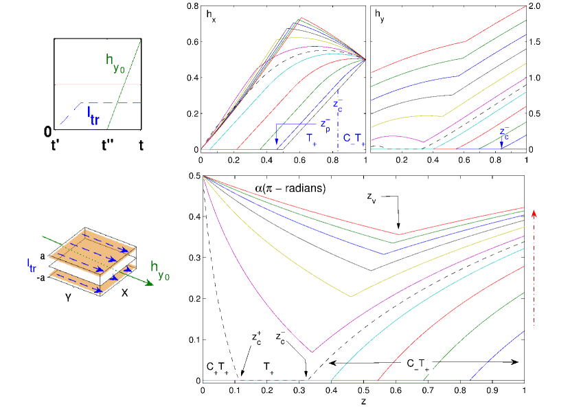
Figure 5.2: Left pane: Schematic representation of the simplest experimental configuration of the longitudinal transport problem which is solved by analytical methods. Right pane Penetration profiles of the magnetic field components and rotation angle in the longitudinal transport experiment ($h_{z0}=0$) for a superconducting slab of thickness $2a$, as calculated from Eq. (5.1). The zone structure induced by increasing the field $h_{y0}$ is marked upon some of the curves. The dashed line corresponds to the transition regime between the states $O/T_{+}/C_{-}T_{+}$ to the unstable regime of states $C_{+}T_{+}/T_{+}/C_{-}T_{+}$ (see text).

In detail, our experimental process starts with the application of the transport current along the y-axis (see left pane of Fig. 5.2) which produce a T₊ zone, i.e., the starting profile can be depicted as follows:

$$dh=dz\quad;\quad d\alpha=0$$

$${\Downarrow}\qquad\qquad$$ (5.9)

$$h=h_{x0}+{\tt z}-1\quad;\quad\alpha=0\,,$$

that penetrates from the surface until the point where $h$ equals $0$, i.e.: ${\tt z}_{p0}=1-I_{tr}$. In our units, ${\tt z}_{p0}=0.5$ for $I_{tr}=h_{x0}=0.5$.

On the one hand, an O zone appears in the inner region $0<{\tt z}<{\tt z}_{p0}$ as far as $I_{tr}<1$. On the other hand, unless an external source of magnetic field is switched on, the above situation remains valid. Thus, upon increasing the external field $h_{y0}$, a flux line rotation starts on the surface and the perturbation propagates towards the center in the form of a C_-T₊ zone defined by

$$dh=dz\quad;\quad d\alpha=-\frac{\chi}{h}\,dz\qquad\qquad$$

$${\Downarrow}\qquad\qquad\qquad\qquad\qquad$$ (5.10)

$$h=h_{x0}+{\tt z}-1\;;\;\alpha=\alpha_{0}+\chi{\rm ln}\left[1+\frac{{\tt z}-1}{h_{0}}\right]\,,$$

which covers the range ${\tt z}_{c}^{-}<{\tt z}<1$, defined by $\alpha=0$ $\Rightarrow$ ${\tt z}_{c}^{-}$ $=$ $1+h_{0}$ $[{\rm exp}(-\alpha_{0}/\chi)-1]$ (see Fig. 5.2). The former T₊ zone is pushed towards the center and occupies the interval ${\tt z}_{p}^{-}<{\tt z}<{\tt z}_{c}^{-}$ with ${\tt z}_{p}^{-}=1-h_{0}$. Finally, an O-zone fills the core $0<{\tt z}<{\tt z}_{p}^{-}$ until the condition ${\tt z}_{p}^{-}=0\Leftrightarrow h_{0}=1$ is reached. Then, with further increase of the local component $h_{y0}$, an instability towards the center of the sample consisting of a transient structure that becomes $C_{+}T_{+}/C_{-}T_{+}$ is induced.

In physical terms, flux vortices penetrate from the surface with some orientation given by the components of the vector $(h_{x},h_{y})$. Owing to the critical condition for the penetration of the field $dh/dz=1$, as soon as the modulus reaches the center, flux rotation must take place there. This is needed for accommodating the vector to the condition ${\bf h}({\tt z}=0)=(0,h_{y}({\tt z}=0))$. On the other hand, as the angle variation is determined by the value of $J_{c\parallel}$, a jump is induced at the center, i.e.: $\alpha({\tt z}=0)\to\pi/2$, and the related instability may be visualized by a critical $C_{+}T_{+}/T_{+}/C_{-}T_{+}$ profile (dashed lines at the right pane of Fig. 5.2) in which the field angle decreases from its surface value $\alpha_{0}$ to $0$ in the $C_{-}T_{+}$ region, then keeps null within the $T_{+}$ zone, and suddenly increases to the value $\pi/2$ in the inner $C_{+}T_{+}$ band defined by

$$dh=dz\quad;\quad d\alpha=\frac{\chi}{h}\,dz\qquad\qquad\quad$$

$${\Downarrow}\qquad\qquad\qquad\qquad\qquad$$ (5.11)

$$h=h_{x0}+{\tt z}-1\;;\;\alpha=\pi/2-\chi{\rm ln}\left[1+\frac{{\tt z}}{h_{0}-1}\right]\,.$$

In fact, the $C_{+}T_{+}/C_{-}T_{+}$ structure is stabilized with the intersection between regions at the point [$\alpha^{{+},{+}}({\tt z}_{\rm v})=\alpha^{{-},{+}}({\tt z}_{\rm v})$] given by

$${\tt z}_{{\rm v}}=1-h_{0}+\sqrt{h_{0}(h_{0}-1)}\leavevmode\nobreak\ {\rm exp}\left[\frac{\pi/2-\alpha_{0}}{\chi}\right]\,.$$ (5.12)

Finally, note that upon further increasing $h_{y0}$ the point ${\tt z}_{\rm v}$ follows the rule ${\tt z}_{\rm v}(h_{y0}\to\infty)\to(1+h_{x0}/\chi)/2$

In brief, our simple analytical model allows to identify the following physical phenomena as the longitudinal component of the magnetic field $h_{y0}$ (parallel to the flow direction of the transport current) is increased:

1. The appearance of a surface layer with negative transport current density (mind the slope of $h_{x}$ in Fig. 5.2 in view of Eq. (5.1)).

2. The applied magnetic field re-entry as related to the inner $C_{+}T_{+}$ zone, predicting the occurrence of local paramagnetic states near of the center of the superconducting sample.

These features will be confirmed along the forthcoming section, where the SDCST statements are thoroughly presented and a further comparison with the analytical model of Ref. [13] will be displayed.

5.1.2 The SDCST statement and the BM’s approach

Below, let us introduce an experimental configuration rather to the opposite side of the previous situation, and that may be used for comparison to the work in Ref. [13]. To be specific, based upon our well-known 3D physical scenario for superconductors with magnetic anisotropy, we shall consider the time evolution of magnetic profiles $\textbf{h}_{l+1}(z)$ within an infinite superconducting slab of thickness $2a$ (see Fig. 5.3), cooled under the assumption of an initial state defined by an uniform vortex lattice perpendicular to the external surfaces, i.e., a constant magnetic field $h_{z0}$. In terms of the geometrical interpretation for the material law, the above starting point or initial state corresponds to choose $\theta=0$ in Fig. 4.1 (pag. 4.1). Then, a transport current is injected along the superconducting slab in the direction of the $y-$axis inducing a rotation of the critical current region $\Delta_{\textbf{r}}$ on the plane of currents $xy$ by means the induced magnetic field component $h_{x}$ (i.e., $\theta\neq 0$ in Fig. 4.1). Finally, a third source of magnetic field is switched on along the $y-$axis, which induces a new rotation of the current density vector by means the introduced local component of magnetic field $h_{y}$ (i.e., $\alpha\neq 0$ in Fig. 4.1).

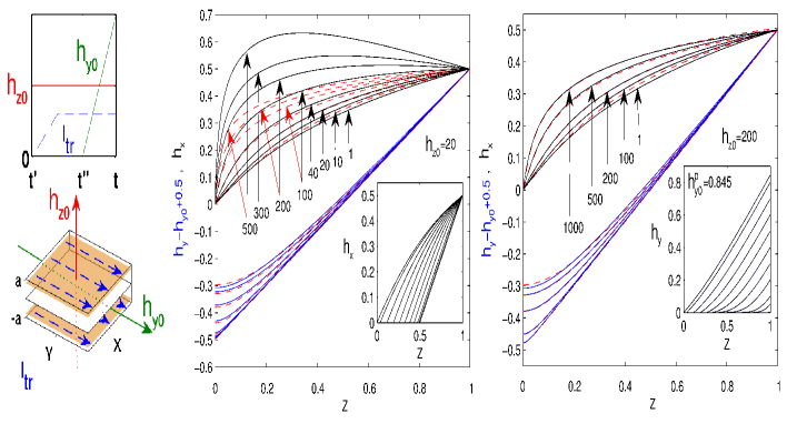
Figure 5.3: Left pane: Schematic representation of the 3D experimental configuration of the longitudinal transport problem in the slab geometry. Central and right panes: Profiles of the magnetic field components $h_{x}(z)$ and $h_{y}(z)$ for the longitudinal problem corresponding to a transport current along the $y$ axis of value $I_{\rm transport}\equiv J_{c\perp}a/2=0.5$ and at several increasing values of the magnetic field $h_{y0}$ as labeled in the curves. Here, we have assumed an uniform perpendicular field $h_{z0}=20$ (central pane) and then $h_{z0}=200$ (right pane). The plot shows the comparison of the full range numerical solution in the infinite widthband model or so-called T-state model (continuous lines) to the analytical approximation in Eq. (5) (dashed). The insets show the initial flux penetration profiles for both components of the magnetic field.

It is worth mentioning that, by symmetry, the current density is confined to the $xy$-plane, such that the distribution of the current can be displayed in a proper set of circuits naturally defined by a collection of in-plane current layers located at the heights $z_{i}$, and each one carrying a current density given by $[J_{x}(z_{i}),J_{y}(z_{i})]$ which must satisfy a certain set of physical constraints. In particular, this means that in practice one should impose the restriction that ${\bf J}$ belongs to the projection of the critical current region onto the plane (${\bf J}\in\Delta_{p}$) and that $\nabla\cdot\textbf{J}\equiv 0$. As a main fact it will be established that, when building the parallel configuration, the response of the superconductor depends on the limitations for the current density established by the depinning threshold $J_{c\perp}$ on the orientation of the local magnetic field, and eventually on the threshold value for the cutting component or $J_{c\parallel}$. This is easily understood at a qualitative level just by glancing once more the left-side of Fig. 4.1 (pag. 4.1). Within this picture, with transport current density flowing along the $xy$-plane, notice that for moderate values of the angle $\theta$ between the local magnetic field and the $z$-axis, the critical current restriction or material law $\Delta_{\rm p}$ becomes an ellipse of semi-axes $J_{c\perp}$ and $J_{c\parallel}^{\rm p}$ with

$$J_{c\parallel}^{\rm p}={J_{c\perp}}/{\cos{\theta}}=J_{c\perp}{\sqrt{H_{x}^{2}+H_{y}^{2}+H_{z}^{2}}}/{H_{z}}\,.$$ (5.13)

An increase of the in-plane magnetic field component will result in a tilt of the cylinder by an increase of the angle $\theta$. In particular notice that, initially the maximum value of the in-plane parallel current density, $J_{c\parallel}^{\rm p}$, grows with the angle $\theta$, independent of $J_{c\parallel}$ (which is, thus, absent from the theory) until the maximum value $\sqrt{J_{c\perp}^{2}+J_{c\parallel}^{2}}$ is reached. Then, the ellipse is truncated and eventually would be practically a rectangle of size $2J_{c\parallel}\times 2J_{c\perp}$ when $\gamma\to\pi/2$. Outstandingly, for large values of $\chi\equiv J_{c\parallel}/J_{c\perp}$ (long cylinders), the critical current along the parallel axis $J_{c\parallel}^{\rm p}$ increases more and more as the weight of $H_{z0}$ decreases, and furthermore, this quantity is always beyond the individual values $J_{c\perp}$ and $J_{c\parallel}$.

Recall that the variational statement for three dimensional configurations on the slab geometry has been thoroughly discussed in chapter 4.1. Thus, based on the numerical resolution for discretized layers, and within the mutual inductance formulation [Eq. (3.3)], the above described longitudinal problem takes the following form:

$${\cal F}[I_{l+1}]= \leavevmode\nobreak\ \frac{1}{2}\sum_{i,j}I_{i,l+1}^{x}{\rm M}_{ij}^{x}I_{j,l+1}^{x}-\sum_{i,j}{\rm I}_{i,l}^{x}{\rm M}_{ij}^{x}I_{j,l+1}^{x}$$ (5.14)

$$+\frac{1}{2}\sum_{i,j}I_{i,l+1}^{y}{\rm M}_{ij}^{y}I_{j,l+1}^{y}-\sum_{i,j}{\rm I}_{i,l}^{y}{\rm M}_{ij}^{y}I_{j,l+1}^{y}$$

$$+\sum_{i}I_{i,l+1}^{y}(i-1/2)({\rm h}_{0,l+1}^{y}-{\rm h}_{0,l}^{y})\,.$$

Moreover, we already know that the local components of the magnetic fields have to be evaluated according to equations of the kind (4.1) & (4.2), and the parallel and perpendicular projections of the sheet current components are given by

$$I_{\perp}^{2}=\left(1-(h_{i}^{x})^{2}\right)(I_{i}^{x})^{2}+\left(1-(h_{i}^{y})^{2}\right)(I_{i}^{y})^{2}-2h_{i}^{x}h_{i}^{y}I_{i}^{x}I_{i}^{y}\,,$$ (5.15)

and

$$I_{\parallel}^{2}=(h_{i}^{x}I_{i}^{x})^{2}+(h_{i}^{y}I_{i}^{y})^{2}+2h_{i}^{x}h_{i}^{y}I_{i}^{x}I_{i}^{y}\,.$$ (5.16)

Technically, the main differences with the problems considered in the above chapter are the inclusion of an additional constraint for the transport current, and new expressions for the inductance matrices.

On the one hand, for our problem with transport current, one has to consider for each temporal step the external constraint

$$\sum_{i}I_{i}^{y}(t)=I_{tr}(t)\,.$$ (5.17)

On the other hand, as related to the symmetry properties for the transport configuration [$I_{i}^{y}(z)=I_{i}^{y}(-z)$ as opposed to the antisymmetry for the case of shielding currents], here one has to use the mutual inductance expressions

$$M_{i,j}^{x}\equiv 1+2\left[min\{i,j\}\right]\,\qquad\,,\qquad M_{i,i}^{x}\equiv 2\left(\frac{1}{4}+i-1\right)\,,$$

(5.18)

$$M_{i,j}^{y}\equiv 1+2\left[N_{s}-max\{i,j\}\right]\,\qquad\,,\qquad M_{i,i}^{y}\equiv 2\left(\frac{1}{4}+N_{s}-i\right)\,.$$

with $N_{s}$ the full number of layers in the discretized slab.

Finally, within the framework of the SDCST, it is to be recalled that the local components of the current density have to be constrained according to one of the models contained by our generalized material law depicted in the right pane of Fig. 4.1 (pag. 4.1) [Mathematically see Eq. (2.19), pag. 2.19]. Thus, with the aim of achieving a comparison between our numerical results and the analytical approach of Ref. [13], in Fig. 5.3 we show some of the results for the T-states assumption under consideration of a strong perpendicular field $h_{z0}=200$, and the arising discrepancies when a perpendicular field of moderate intensity (e.g., $h_{z0}=20$) is considered.

Firstly, let us emphasize that within our SDCST there is no restriction for the ratios $\chi^{-1}\equiv J_{c\perp}/J_{c\parallel}$ and $\varsigma\equiv J_{c\perp}a/H_{z0}$, which become small parameters within the analytical approach of Ref. [13]. Notice that the smallness of $\chi^{-1}$ means that the arising critical state is approximated by the unbounded band region $|j_{\perp}|=1,0<|j_{\parallel}|<\infty$ described in the chapter 4.6 (T-states). The smallness of $\varsigma$ was meant to indicate a small deviation of the full magnetic field respect to the $z-axis$. Then, moderate values of $j_{\parallel}$ are expected. Notoriously, the above hypotheses of Ref. [13] allow to state the problem by a set of approximate analytic formulas for the electromagnetic quantities which in turn allow to bypass the numerical solution of the differential equations. However, as it will be shown below, the range of application is narrower than expected.

Figure 5.3 shows the comparison between the penetration profiles for the local magnetic field components $h_{x}$ and $h_{y}$ obtained from our SDCST with $\chi\rightarrow\infty$ and $j_{c\perp}=1$, and from the analytic expressions in Ref. [13], i.e.,

$$h_{x} = \frac{\alpha}{{\rm cos}\,\theta}{\rm arcsinh}\left(\frac{z}{\alpha}\right)$$

$$h_{y} = h_{y0}-\alpha\left(\sqrt{1+\frac{1}{\alpha^{2}}}-\sqrt{1+\frac{z^{2}}{\alpha^{2}}}\right)$$

$${\rm cos}\,\theta = 2\alpha\,{\rm arcsinh}\left(\frac{1}{\alpha}\right)\,.$$ (5.19)

Here, $\alpha$ has to be obtained for each value of the applied field from the condition $cos\theta=h_{z0}/\sqrt{h_{z0}^{2}+h_{y0}^{2}}$. One can notice that the agreement is rather good for the higher value of the perpendicular field $h_{z0}=200$ (right pane of Fig. 5.3), whereas remarkable differences appear for a moderate field $h_{z0}=20$ as $h_{y0}$ increases (central pane of Fig. 5.3). Our interpretation of the above facts is as follows.

On the one hand, as regards to the establishment of the full penetration profile, we have straightforwardly obtained this condition through the step-by-step integration starting from the state $h_{y0}=0$ (the evolution is shown in the insets of the Fig. 5.3). Whereas the value 0.796 is estimated for the penetration field $h_{y0}^{p}$ within the analytical approach of Ref. [13], by the straightforward method described above we get $h_{y0}^{p}=0.845$. Remarkably, in spite of some small differences for the low field profiles $h_{x}$ and $h_{y}$, at moderate values of the transverse field ($h_{y0}<h_{z0}$) the curves always coincide. On the other hand, the failure of the analytical approximation for the higher values of $h_{y0}$ is readily explained by the observation of the plot. Thus, increasing $h_{y0}$ compresses the transport current towards the center of the sample (as indicated by the slope of $h_{x}(z)$). For the case of $h_{z0}=20$ (central pane of Fig. 5.3), one gets $j_{y,max}\approx 5$ when $h_{y}\approx 100$ and $j_{y,max}\approx 50$ when $h_{y}\approx 1000$, then a considerable value of $j_{\parallel}$ is obtained. This leads to a not so good approximation from the analytic condition in the approximation of Ref. [13], which one is only valid for small values of this quantity. However, when comparison is made for $h_{z0}=200$, one gets $j_{y,max}\approx 1$ when $h_{y}\approx 100$ and $j_{y,max}\approx 5$ when $h_{y}\approx 1000$. Then, a much better performance is obtained for the analytical limit even for very high applied fields $h_{y0}$.

In brief, from the above discussion we may conclude that our SDCST overcomes previous limitations related to the weak longitudinal current conditions. By contrast, in the following section we will show a wide set of numerical calculations for material laws even most complicated than the simplest T-state model here considered, allowing to display the corrections needed in the general critical states.

  5.2 Magnetic anisotropy and the uncommon effects

This section will be devoted to unveil the features of longitudinal transport problems under general critical state conditions, and to identify the influence of a number of physical parameters along the different stages of the magnetization process. Here, for the experimental configuration depicted in the left pane of Fig. 5.3 and based on the numerical resolution of the variational statement, a complete tour along the whole set of values for the perpendicular field will be presented. We shall concentrate on the effect of the flux cutting boundary ($j_{c||}$) considering several conditions for the material law introduced by our SDCST (see left pane at Fig. 4.1, pag. 4.1). Firstly, the extreme case $\chi\to\infty$ or infinite bandwidth model (T-states model) will be considered (Subchapter 5.2.1). Secondly, several anisotropic models characterized by the superelliptic relation [Eq. (2.19), pag. 2.19]

$$j_{\perp}^{2n}+(j_{\parallel}/\chi)^{2n}\leq 1$$ (5.20)

will be thoroughly analyzed (Subchapter 5.2.2). In particular, we will set of material laws defined by the parameters $\chi=1$, 2, 3, and 4 with the smoothing index n=4.

Remarkably, our procedure will reveal the fingerprints of the cutting and depinning mechanisms, thus being a theoretical pathway for the reconstruction of the material law, represented by the proper region $\Delta_{\textbf{r}}$.

5.2.1 Extremal case: The T-states model

The T-state model for three dimensional configurations of the applied magnetic field has been exhaustively studied in chapter 4.3. Here, although the depicted scenario is similar, the assumption of a longitudinal transport current allow a straightforward understanding of the physical scopes of this model beyond the analytical approximations. First, we will analyze the properties of the local field [$\textbf{h}(z)$] and the current density profiles [$\textbf{j}(z)$] for a longitudinal configuration built in the fashion described in the left pane of Fig. 5.3 (a third component of the magnetic field $h_{z0}$ is incorporated).

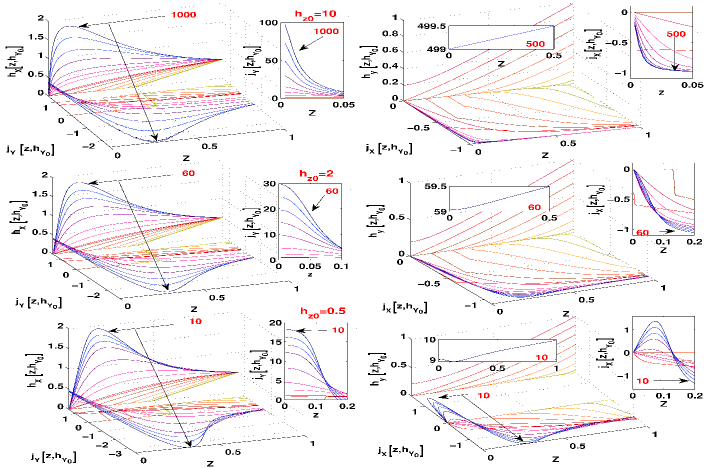
Figure 5.4: Profiles of the local magnetic field components $h_{x}[z,h_{y0}]$ and $h_{y}[z,h_{y0}]$, and the corresponding current-density profiles $j_{y}[z,h_{y0}]$ and $j_{x}[z,h_{y0}]$ for the T-state model and perpendicular magnetic field components $h_{z0}=10$ (top), $h_{z0}=2$ (middle) and $h_{z0}=0.5$ (bottom). The different curves correspond to the following sets of values for the applied longitudinal field at the surface: (i) top row: $h_{y0}=0.005,0.050,0.170,0.340,0.500,0.680,0.845,1.0,40.0,80.0,150.0,300.0,500.0,750.0$, $1000$, (ii) middle row: $h_{y}(a)=0.0050.050,0.170,0.340,0.500,0.680,0.845,1.0,5.0,10.0$, $20.0,30.0,40.0,50.0,60.0$, (iii) bottom row: $h_{y}(a)=0.001,0.050,0.170,0.340,0.500$, $0.680,0.845,1.0,2.0,3.0,5.0,7.0,8.0,9.0,10.0$. Insets to the middle pane correspond to the $j_{y}[z,h_{y0}]$ profiles closer to the center of the sample. Analogously, insets to the right correspond to the $j_{x}[z,h_{y0}]$ profiles. Finally, inner insets at right pane correspond to a specific profile of $h_{y}[z,h_{y0}]$ so as to highlight the occurrence of magnetic field reentry at low values of $h_{z0}$.

Fig. 5.4 shows the behavior of the magnetic field profiles and the induced currents subsequent to the application of the transport current for three different initial conditions: $h_{z0}=10$, $h_{z0}=2$, and $h_{z0}=0.5$, all of them under assumption of the T-state model. The initial state for the transport current condition ($I_{tr}=J_{c\perp}a/2$) establishes the initial transport profile $j_{y}\{0\leq z<a/2\}=0$ and $j_{y}\{a/2\leq z\leq a\}=1$. As the transport current is no longer modified, the condition $h_{x}(a)=0.5$ can be applied in what follows. On the other hand, by symmetry, one has the condition $h_{x}(0)=0$ at the center of the slab.

In detail, when the external magnetic field $[h_{y0}=h_{y}(a)]$ (the applied parallel field) is linearly increased from $h_{y}(a)=0$, a current density $j_{x}$ is induced from the superconducting surface as an effect of Faraday’s law. Simultaneously, the local component of the magnetic field $h_{x}(z)$ increases monotonically following two continuous stages fulfilling the aforementioned boundary conditions. First, the superconducting sample is fully penetrated by the transport current when $h_{y}^{\star}(a)=0.845\pm 0.003$ and eventually, the condition $j_{y}(0)=1$ is reached as soon as $h_{y}(a)\rightarrow 0.860$. We notice that the value of $h_{y}^{\star}(a)$ for the full penetration profile is basically independent of $h_{z0}$ (at least to the numerical precision of our numerical calculations), in agreement with our analytical solution [33] introduced in the previous section (Chapter 5.1.1). Second, a remarkable enhancement of the transport current density occurs around the center of the slab as $h_{y}(a)$ increases beyond $h_{y}^{\star}(a)$. Furthermore, an eventual negative current density appears shielding the positive transport current around the center of the slab. It is to be noticed that the appearance of negative current flow is enhanced when the magnetic component $h_{z0}$ is decreased (Fig. 5.5).

It is noteworthy that for the range of values $h_{z}(0)<h_{y}^{\star}(a)$ negative surface current appears even for the partial penetration regime, e.g., for $h_{z0}=0.5$ one has $j_{y}(a)<0$ for $h_{y}(a)>0.722$. Further, another outstanding property is the occurrence of profiles with magnetic field reentry (paramagnetism in the component $h_{y}$ around the center of the slab) for $h_{z0}\lesssim 1$ and under relatively low applied magnetic fields $h_{y}(a)$ (see Fig. 5.4). In fact, we call the readers’ attention that the above mentioned effects, local paramagnetism and negative current zones, have both been shown analytically in the limiting case $h_{z0}=0$ (Chapter 5.1.1). Along this line, as a general rule, we can conclude that the smaller the value of $h_{z0}$, the sooner the surface of negative transport current and even paramagnetic local effects appear.

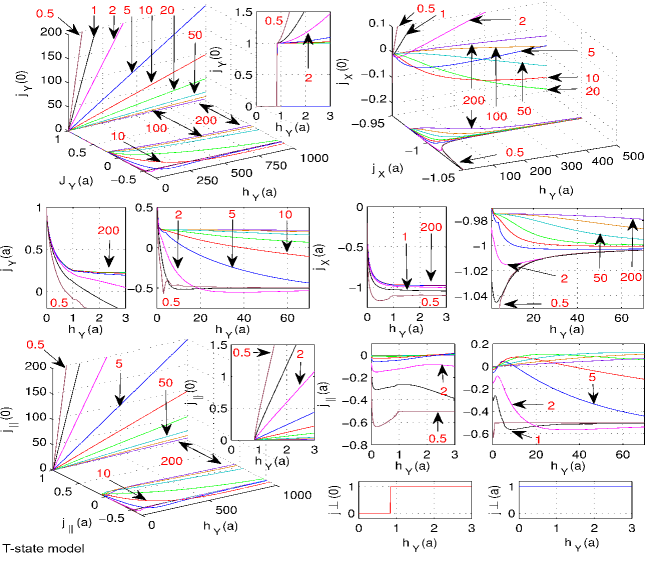
Figure 5.5: Dynamics of the local current density as a function of the applied longitudinal magnetic field $h_{y0}=h_{y}(a)$ along the central and external sheets of the slab. The results are shown for the T-state model ($J_{c||}\to\infty\leavevmode\nobreak\ \&\leavevmode\nobreak\ J_{c\perp}=1.0$). Top: the components $j_{y}$ and $j_{x}$ at $(z=0)$ and $(z=a)$. Middle: details of the above behavior. Bottom: dynamics of the parallel and perpendicular components of $\bf j$ in the same conditions as above. The different curves correspond to the values of the perpendicular magnetic field given by $h_{z0}=0.5,1,2,5,10,20,50,100,200$. Several scales have been displayed to avoid information loss with all plots running over the same color scale.

On the other hand, figure 5.5 displays the evolution of the current density vector focusing us on the specific values at the superconducting surface ($z=a$) and at the center of the superconducting slab ($z=0$) as the longitudinal magnetic field $h_{y}(a)$ is increased. Outstandingly, the involved physical features are straightforwardly explained by the polar decomposition of the current density introduced in chapter 4.1 [See Eqs. (4.6) - (4.8), pag. 4.6]. In brief, notice that the unbounded parallel current density allows unconstrained rotations for the flux lines as the applied magnetic field increases. In particular, this leads to negative values of $j_{y}(a)$ (slope of $h_{x}(a)$), simultaneous to high $j_{y}(0)$ (slope of $h_{x}(0)$). Moreover, it should be noticed that negative values of the transport current are favored by smaller and smaller values of the field component perpendicular to the surface of the sample $h_{z0}$. Also, notice that at the center of slab the flux line dynamics is mainly governed by the longitudinal transport current density $j_{y}(0)$. The basic idea is that for moderate values of $h_{z}$, when $h_{y}$ increases $j_{y}$ practically becomes $j_{\parallel}$. As this component is unconstrained, it grows indefinitely at the center.

For a closer connection with real experiments, below let’s concentrate on the magnetostatic properties by means of the global sample’s magnetization curve M(H). Thus, we have calculated M as a function of the longitudinal magnetic field $h_{y}(a)$.

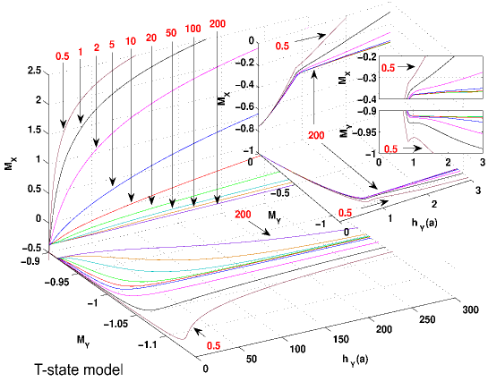
Figure 5.6: The magnetic moment components $(M_{x},M_{y})$ of the slab as a function of the applied magnetic field component $h_{y}(a)$ for the T-state model. The curves are labeled according to the perpendicular magnetic field $h_{z0}=0.5,1,2,5,10,20,50,100,200$. The insets show different zooms of the magnetic moment components for low values of the applied longitudinal field. The same color scale applies to all the plots.

Fig. 5.6 displays the magnetic moment components $M_{x}(h_{y0})$ and $M_{y}(h_{y0})$ in units of $J_{c\perp}a^{2}$. First, notice that within the partial penetration regime ($h_{y}(a)\leqslant h_{y}^{\star}(a)$) the magnetic moment components are almost independent of the perpendicular magnetic field $h_{z0}$ (at least for non small values of this quantity). On the contrary, when $h_{z0}<1$ and the patterns of negative current even occur before the fully penetrated state, the magnetization slightly increases. This is accompanied by faint field reentry effects that are also shown within the figure. Furthermore, as the threshold cutting current density $j_{c\parallel}$ is unbounded for the T-state model, the magnetic moment $M_{x}$ always increases as related to the diverging behavior of $j_{y}(0)$.

Let us emphasize that, as the unbounded behavior for the parallel current density assumed above leads to the prediction of arbitrarily high values of the transport current density, consequently the T-state model must be physically reconsidered. For example, on the one hand, the trend of the magnetic moment $M_{x}$ and also the unbounded longitudinal current density $j_{y}$ disagree with the experimental evidences recollected in Refs. [7, 35, 36, 42, 45, 29, 17, 30, 31, 32]. On the other hand, in Fig. 5.5 one can observe that, as soon as the flow of negative current along the superconducting surface is reached, it never disappears notwithstanding the longitudinal magnetic field remains increasing. By contrast, the disappearance of the patterns of superficial negative current were detected in Refs. [21, 22, 23, 39, 42, 45]. These observations have lead to consider $j_{c\parallel}$ bounded descriptions as satisfactory solutions of the peculiar phenomena involved on the longitudinal transport current problem [35, 36, 21, 22, 23]. Rather recent experimental data on high temperature superconductors [15, 16] also indicate that physical bounds are to be considered for both components of the critical current.

Thus, as will be described below in section 5.2.2, our generalized SDCST suits the necessity of dealing with a physically acceptable description of both local and global issues about the electromagnetic quantities involved in the longitudinal transport current problem [2, 33, 34].

5.2.2 Material laws with magnetic anisotropy: CT$\chi$ – models

More realistic models for the material law are presented below. Henceforth, we shall use the simplified notation T or CT$\chi$ as regards to the infinite bandwidth model (T by transport) or the superelliptical critical state models with anisotropy $\chi=|J_{c||}/J_{c\perp}|$ (CT by cutting and transport, and $\chi$ the index controlling the magnetic anisotropy of the model). Recall that neither the isotropic model (n=1) nor the rectangular models ($n\rightarrow\infty$) are able to achieve a full explanation of the involved physical events. Thus, hereafter a value $n=4$ will be chosen for the smoothing index, corresponding to an intermediate regime between the above mentioned material laws. As an additional advantage, we want to mention that, technically, the use of smooth models produces stable and faster numerical convergence.

In order to obtain continuity with the T-state results obtained above, the electrodynamic quantities of interest have been obtained under the same experimental configuration shown at the left pane of Fig. 5.3, and a similar analysis scheme to that developed in the previous section will be tackled here. Thus, with the aim of getting a detailed physical interpretation on how the longitudinal and transverse magnetic fields affect the dynamics of the transport current problem, we will show the magnetic penetration profiles for low and high perpendicular fields, i.e., $h_{z0}=0.5$ (Figs. 5.7 & 5.8) and $h_{z0}=10$ (Figs. 5.9 & 5.10), for different $CT\chi$ conditions. Then, for completeness, the set of initial conditions $h_{z0}$ is extended in Figs. 5.11 & 5.12, by means a thorough analysis of the dynamics of the current density over the central layer $[j_{y}(z=0)]$ and external layer $[j_{y}(z=a)]$ of the slab. Finally, it will be shown that the fingerprint of the different CT$\chi$ models is identified as a peak effect in the curves for the magnetic moment components (Fig. 5.13 & 5.14) caused by the maximal enhancement of the transport current density along the central layer.

( A. ) Penetration Profiles and current density behavior

On the one hand, let us recall that under the SDCST the square condition is given by $\chi=1$ (CT1) assuming the customary condition $J_{c\perp}=1$ (i.e., $j_{c\parallel}=1$ as $\chi\equiv J_{c\parallel}/J_{c\perp}$). This can be considered as a lower bound for such quantity because the experimental values reported in the literature are typically above unity. On the other hand, as we have observed an intricate behavior for the local dynamics of the electromagnetic quantities under the CT$\chi$ conditions, henceforward, we will split the experimental process in three successive stages as the longitudinal magnetic field component $h_{y}(a)$ is increased. We mean:

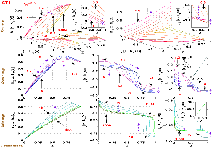
Figure 5.7: Profiles of the magnetic field components $h_{x}[z,h_{y0}]$ and $h_{y}[z,h_{y0}]$ for a perpendicular field component $h_{z0}=0.5$. Also included are the corresponding current-density profiles $j_{y}[z,h_{y0}]$ and $j_{x}[z,h_{y0}]$ for the CT1 model. For clarity, the longitudinal magnetic field is applied in three stages: Top, $h_{y}(a)=$0.005, 0.050, 0.170, 0.340, 0.500, 0.680, 0.845, 1.0, 1.1, 1.3; Middle, $h_{y}(a)=$1.3, 1.6, 1.9, 2.2, 3.0, 4.0, 5.0, 6.0, and Bottom $h_{y}(a)=10,20,40,80,100,125,150,1000$. Insets at top pane show a zoom of the current density profiles close the external sheet of the superconducting slab. Insets at either middle or bottom panes show the shape of one of the profiles $h_{y}[z,h_{y}(a)]$ for the corresponding stage. Dashed line arrows are included to supply a trace method from the initial profile until the last one, in correspondence to the aforementioned stages.

• The current density at the center $j_{y}(0)$ increases until a maximum value is obtained. The set of profiles for the physical quantities [$h_{x}(z)$,$j_{y}(z)$] and [$h_{y}(z)$,$j_{x}(z)$] in the partial penetration regime are also included within this stage (see e.g. top of Figs. 5.7 - 5.10). The occurrence of possible negative values for the longitudinal current density along the superconducting surface $j_{y}(a)$ is also focused for low values of the perpendicular magnetic field $h_{z0}$.

• The longitudinal current density profiles $j_{y}(z)$ show a bow tie pattern, whose evolution is shown until the minimum value for the longitudinal current density along the superconducting surface, $j_{y}(a)$, is reached (see e.g., the middle row of Figs. 5.7 - 5.10).

• Eventually, the longitudinal current density $j_{y}(a)$ grows up by increasing the longitudinal applied field $h_{y}(a)$, and further it stabilizes around a certain value (e.g., $j_{y}(a)\approx 0.5$ for CT1 case as it is shown in the bottom of Figs. 5.7 - 5.9).

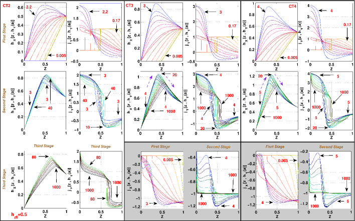
Figure 5.8: Profiles of $h_{x}[z,h_{y0}]$ and $j_{y}[z,h_{y0}]$ for the 1st (top) and 2nd (middle) stages of the magnetic dynamics described in the cases CT2 (left pane), CT3 (central pane) and CT4 (right pane), all under a field $h_{z0}=0.5$. The 3rd stage is only defined for the CT2 case (left pane - bottom), as we have not noticed remarkable difference between the 2nd and 3rd stages for cases CT3 and CT4, at least for values of the longitudinal applied field not beyond of $h_{y}(a)=1000$. So, in return, the lower panes in cases CT3 and CT4 show the profiles for $j_{x}[z,h_{y}(a)]$ for the 1st and 2nd stages. $h_{y}(a)$ is as follows. CT2: (1st stage) $h_{y}(a)=$0.005, 0.050, 0.170, 0.340, 0.500, 0.680, 0.845, 1.0, 1.1, 1.3, 1.6, 1.9, 2.2; (2nd stage) $h_{y}(a)=$3, 4, 5, 6, 8, 10, 20, 40; and (3rd stage) $h_{y}(a)=$ 80, 120, 160, 200, 300, 400, 600, 800, 1000. CT3: (1st stage) $h_{y}(a)=$0.005, 0.050, 0.170, 0.340, 0.500, 0.680, 0.845, 1.0, 1.5, 1.8, 2.2, 2.6, 3.0; and (2nd stage) $h_{y}(a)=$4, 5, 6, 8, 15, 20, 40, 70, 100, 150, 200, 300, 400, 600, 1000. CT4: (1st stage) $h_{y}(a)=$0.005, 0.050, 0.170, 0.340, 0.500, 0.680, 0.845, 1.0, 1.5, 1.8, 2.2, 2.6, 3.0, 4.0; and (2nd stage) $h_{y}(a)=$5, 6, 8, 15, 20, 40, 100, 200, 400, 600, 1000.

As far as concerns to the field and current density penetration profiles, it is to be noticed that the trend of the profiles for the partial penetration regime is fairly independent of the perpendicular magnetic field $h_{z0}$ (Figs. 5.7 - 5.10). Moreover, the partial penetration regime in which the transport current zone progressively penetrates the sample is nearly independent of the magnetic anisotropy of the critical state (compare the above profiles to their respective ones for the T-state condition in Fig. 5.4).

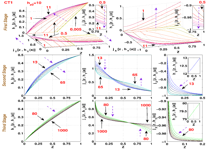
Figure 5.9: Same as Fig.5.7, but for $h_{z0}=10$ and the values of the longitudinal field: (Top) $h_{y}(a)=$ 0.005, 0.050, 0.170, 0.340, 0.500, 0.680, 0.845, 1.0, 4.0, 6.0, 8.0, 11, (Middle) $h_{y}(a)=$ 13, 15, 17, 20, 25, 35, 50, 65, (Bottom) $h_{y}(a)=$ 80, 100, 125, 150, 200, 300, 400, 1000.

We call readers’ attention to the fact that, in the aforementioned first stage, the negative current patterns are also found under the low applied magnetic fields $h_{z0}<0.5$. However, by contrast to the results within the previous section, it is to be recalled that for the T-state model the condition $j_{c||}\rightarrow\infty$ allows unbounded values for the longitudinal current $j_{y}$ at the center of the sample. By contrast, for the bounded cases CT$\chi$, the magnetic anisotropy of the material law $\Delta_{r}$ defines the maximal current density for the critical state regime. In other words, the maximal length of the vector j corresponds to the optimal orientation of the region $\Delta_{r}(\chi,n)$ in which the biggest distance into the superelliptical condition is reached, i.e., such situation corresponds to the maximal transport current allowed in the superconductor, and can be calculated by the following analytical expression

$${\rm Max}\{j_{c\parallel}(\Delta_{\textbf{r}})\}=j_{y}^{max}=\left(1+\chi^{2n/(n-1)}\right)^{(n-1)/2n}\,.$$ (5.21)

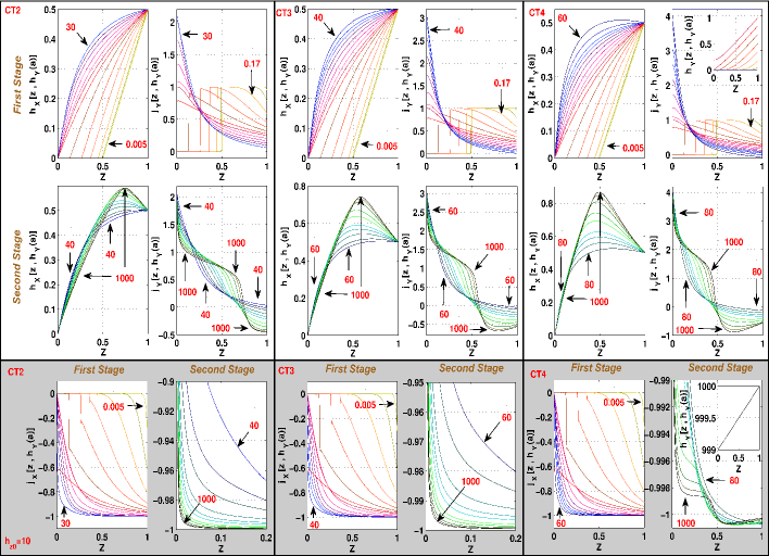
Figure 5.10: Similar to Fig. 5.8, but for $h_{z0}=10$. The curves are labeled as follows. CT2 (left pane): 1st stage (top) $h_{y}(a)=$ 0.005, 0.050, 0.170, 0.340, 0.500, 0.680, 0.845, 1.0, 5.0,10, 15, 20, 30, and 2nd stage (middle) $h_{y}(a)=$ 40, 60, 80, 120, 160, 200, 300, 400, 600, 800, 1000. CT3 (middle pane): 1st stage (top) $h_{y}(a)=$ 0.005, 0.050, 0.170, 0.340, 0.500, 0.680, 0.845, 1.0, 5.0, 10, 15, 20, 25, 30, 40, and 2nd stage (middle) $h_{y}(a)=$60, 80, 120, 160, 200, 300, 400, 600, 800, 1000. CT4 (right pane): 1st stage (top) $h_{y}(a)=$0.005, 0.050, 0.170, 0.340, 0.500, 0.680, 0.845, 1.0, 5.0, 10, 15, 20, 35, 30, 40, 60, and 2nd stage (middle) $h_{y}(a)=$ 80, 120, 160, 200, 300, 400, 600, 800, 1000. In the bottom of panes CT2, CT3 and CT4, the corresponding profiles of $j_{x}[z,h_{y}(a)]$ are shown.

( B. ) Central and superficial patterns of the current density

Note that Eq. 5.21 allows us to obtain the maximum value expected for $j_{y}$ in terms of the actual critical state model in use. Thus, as we have assumed n=4 for the different CT$\chi$ models considered here, one gets $j_{y}^{max}=1.2968$ for the CT1 case, $j_{y}^{max}=2.1127$ for the CT2 case, $j_{y}^{max}=3.0591$ for the CT3 case, and $j_{y}^{max}=4.0369$ for the CT4 case. These values may be checked by means our numerical results in Figs. 5.11 & 5.12 for the intensity of the transport current density in the central layer of the slab, i.e., the obtained patterns $j_{y}(0)$.

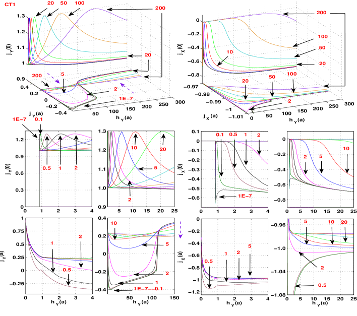
Figure 5.11: Evolution of the current density vector for the CT1 model. To the left, we show the patterns of transport current over the central layer ($j_{y}(z=0)$) and external layer ($j_{y}(z=a)$) of the slab. To the right, we show the variation of the perpendicular component $j_{x}(z=0)$ and $j_{x}(z=a)$. The curves are labeled according to the perpendicular magnetic field component $h_{z0}=$ 0.1, 0.5, 1, 2, 5, 10, 20, 50, 100, 200.

In addition, note that by a thorough analysis of the current density components along the central ($z=0$) and external layers ($z=|a|$) of the superconducting slab, several remarkable physical properties can be straightforward depicted (Figs. 5.11 & 5.12). On the one hand, notice that the full penetration regime can be clearly distinguished from the partial penetration regime, and remarkably the emergence of negative states for the transport current density close to the external surface of the superconducting sample it is more evident either when $h_{z0}$ is reduced and/or the current density anisotropy factor $\chi$ is increased. On the other hand, outstandingly the maximal value of the current density along the original direction of the transport current ($y-$axis) can be depicted in terms of $j_{y}(0)$, where its maximal value defined by Eq. (5.21) turns out to be independent of the perpendicular applied magnetic field at least as regards the existence of the peak effect in the transport current density. Thus, the enhancement of the transport current density can be either accelerated or decelerated with the tilt of the applied magnetic field, but in general terms, its maximum directly relates to the limitation introduced by the cutting mechanism. Physically, this means that the role played by the magnetic anisotropy of the material law may be characterized by the influence of the threshold cutting value on the enhancement of the critical current density.

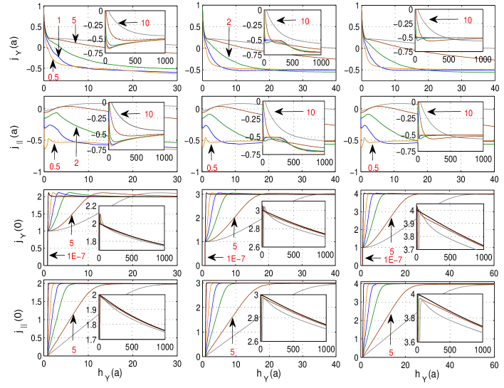
Figure 5.12: Dynamics of the current density vector for the models CT2 (left pane), CT3 (middle pane) and CT4 (right pane). The first row of plots corresponds to the patterns of transport current along the surface layers of the slab [$j_{y}(z=a)$]. The second one, corresponds to the respective values for the parallel component of the current density [$j_{||}(a)$]. The dynamics of the transport current $j_{y}$ and the component $j_{||}$ at the central layer of the superconducting slab $(z=0)$ is shown at the third and fourth rows, respectively. The curves are labeled according to the perpendicular magnetic field component $h_{z0}=$1E-7, 0.5, 1, 2, 5, 10 with all plots having the same color scheme.

In order to confirm the above physical interpretation, in Fig. 5.12 we show the magnetic dynamics of the longitudinal current density $j_{y}$, and the cutting current component $j_{||}$ for the conditions CT2, CT3, and CT4. We have taken a wide set of values for the perpendicular field component ($h_{z0}$). On the one hand, as far as concerns the sample’s surface, we have observed that the longitudinal current density $j_{y}(a)$ does not display significant differences when one has $\chi\geq 2$ (see also Fig. 5.5 for the T-state model with $\chi\rightarrow\infty$). Hence, the disappearance of the negative current flow along the external superconducting surface does not occur despite a very high applied magnetic field has been considered ($h_{y}(a)=1000$). On the other hand, it is important to notice that the patterns of the parallel current density along the superconducting surface ($j_{||}(a)$) are almost indistinguishable as soon as the condition $\chi\geq 2$ (CT2) is reached (upper half of Fig. 5.12). This implies that for an accurate picture of the parallel critical current, surface properties do not provide a useful information.

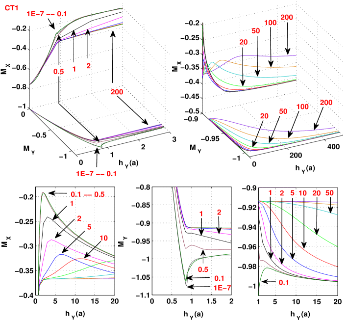
Figure 5.13: Magnetic moment components $M_{x}$ and $M_{y}$ of the slab as a function of the applied magnetic field $h_{y}(a)$ for the CT1 model. The curves are labeled according to the perpendicular magnetic field component $h_{z0}$ for each.

However, Fig. 5.12 shows that the threshold value for the cutting current density can be estimated from the experimental measurement of the transport current density along the central sheet of the superconducting sample. Moreover, regardless to the experimental conditions ($h_{z0}$, $h_{y}(a)$) and also for different bandwidths $\chi$ no significant change occurs in the parallel current density around the central sheet of the sample (lower half of Fig. 5.12).

( C. ) Features on the magnetic moment

Outstandingly, it is to be noticed that the limitation introduced by the flux cutting mechanism imposes a maximal compression of the current density within the sample. Thus, the peak effects both for the transport current density $j_{y}$ (Figs. 5.11 & 5.12) and for the magnetic moment component $M_{x}$ (Figs. 5.13 & 5.14) are defined by the instant at which the maximal transport current density occurs. Additionally, upon further increasing the longitudinal applied magnetic field component $h_{y}(a)$, the profile $h_{x}(z)$ will be forced to decrease from the central sheet ($z=0$) towards the external surface ($z=a$). This reversal generates a local distortion of the longitudinal current density $j_{y}$ in a bow tie shape (see the middle row of Figs. 5.7 & 5.10). Likewise, as soon as the profile $j_{||}(0)=j_{c||}$ is reached, the magnetic moment $M_{x}$ starts decreasing as one can see by comparison of Figs. 5.11 & 5.13 and Figs 5.12 & 5.14.

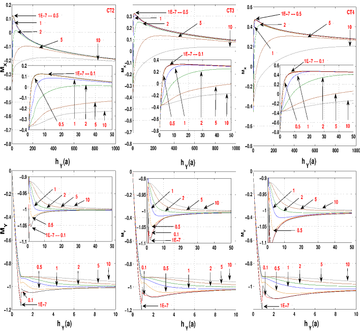
Figure 5.14: Same as Fig. 5.13, but here the curves are corresponding to the CT2 (left pane), CT3 (central pane), and CT4 (right pane) critical state models.

Finally, one additional feature is to be noted: the interval between the instant at which the maximal transport current condition is reached ($j_{y}(0)=j_{y}^{max}$), and the instant at which the slope of the magnetic moment $M_{x}$ changes sign, could be assumed as transient or stabilization period required for an accurate determination of the value $j_{c||}$ when measurements are performed in terms of the applied longitudinal field $h_{y0}=h_{y}(a)$. Apparently, this transient increases with the value of the perpendicular field $h_{z0}$. From this point on, $j_{y}(0)$ may be basically identified with $j_{c\parallel}$.

Chapter 6 Electromagnetism For Superconducting Wires

Type-II superconducting wires are deemed promising elements for large-scale technological applications such as power transmission cables, magnet systems for large particle accelerators, and magnetic-based medical techniques such as MRI. The usefulness of these kind of technology is straightforwardly linked to the local electromagnetic response of the superconductor under variations of the ambient magnetic field and the customary condition of transport-current. Special interest relies on determining the value of the maximum dissipation-free current and characterizing the mechanisms of reduction of electric power dissipation due to alternating fields and/or alternating current flow (commonly called AC losses).

Despite the electric power hysteretic losses associated to a superconducting material are somewhat smaller than the range of power dissipated in normal metals, from the practical point of view, the superconducting technology is still not so attractive to replace the power technology based in copper wires, because in order to keep the temperature of the superconductor below $T_{c}$, heat removal requires a sophisticated and costly cryogenic system. Thus, in order to make the superconducting devices more attractive and competitive with respect to other technologies, it is of utter importance to understand, predict, and eventually, reduce the AC losses of superconducting wires under practical configurations.

Major features of the macroscopic electromagnetic behavior of type-II superconducting wires have been captured in Bean’s model of the critical state [49]. In this framework, magnetization currents of density $\bf J$ are induced within the superconductor during variations of the magnetic flux which accordingly redistribute themselves to screen the penetrating flux within the sample. Their magnitude adopts the critical value $J_{c}$ at a given temperature and specified field. Although simple for idealized configurations, the electrodynamics underlying Bean’s model becomes cumbersome when realistic configurations are addressed. Thus, penetration of magnetic flux must be typically obtained by sophisticated numerical methods.

For example, in order to comprehend the distributions of the field and current in two- and three-dimensional samples subject to time-varying electromagnetic fields a sort of free-boundary problem should be solved. In a superconducting slab or a large cylinder (radius much smaller than their length) exposed either to a parallel magnetic field or a longitudinal transport current, the magnetic field has only one component, and analysis of the field and current distribution is simple [49]. Nevertheless, if the situation is such that the local magnetic field has two components that are functions of two spatial variables, then solving the free-boundary problem for arbitrary relations of the external excitations becomes more and more complicated. In fact, for real applications of superconducting wires, the scenario is such that a simultaneous field and transport current condition must be satisfied. Then, in addition to the ambient field one has the magnetic field generated by the transport current itself [50]. This is the situation, for example, in superconductor windings where each wire is subjected to the magnetic field of its neighboring wires. Thus, as this is the configuration very often met in practice, this chapter is devoted to study round superconducting wires under different configurations of transverse magnetic field and transport current flow.

Subchapter 6.1 is devoted to introduce the theoretical framework of the problem with special attention to the numerical procedure of our variational approach. It is to be noticed that the theoretical statements developed along this section are not only valid for round wires but rather for long superconductors with any topology of the transverse section, e.g., it may include strips of rectangular cross section, wires of elliptical or circular cross section, also any intermediate shape between them, and even multifilament structures as the observed in practical superconducting wires.

Then, in order to introduce our numerical results and to get a fairly clear understanding of the phenomena involved in the dynamics of the electromagnetic quantities for superconducting wires with simultaneous transport current and applied magnetic field, subchapter 6.2 deals with the simpler cases where the superconducting wire is only subjected to a transverse magnetic field in absence of transport current, or on the contrary, assume that the superconducting wire is only subjected to a transport current condition. For a closer connection with the experimental quantities, we have calculated the wire’s magnetic moment (M) and the hysteretic losses ($L$) as a function of AC external excitations, and their comparison with classical analytical approaches are featured. On the other hand, we present a thorough discussion about the observed patterns for the local dynamics of the electromagnetic quantities such as the inner distribution of current density J, the components of the magnetic flux density B and the isolevels of the vector potential A (i.e., the lines of magnetic field), as well as the local distribution of the density of power dissipation $\textbf{E}\cdot\textbf{J}$, whose profiles are displayed at the end of the chapter in the corresponding section of supplementary material.

In subchapter 6.3, numerical simulations of filamentary type II superconducting wires under simultaneous AC transport current and oscillating transverse magnetic field are performed. A wide number of configurations have been considered, with special attention to the aforementioned experimental quantities, M and $L$. On the one hand, according to the temporal evolution of the AC sources, exotic magnetization loops are envisaged. On the other hand, remarkable numerical corrections to several widely used approximate formulae for the hysteretic losses are identified. Also, in view of the differences found between the different cases studied, we present a comprehensive study of the local dynamics of the electromagnetic quantities in analogy to the previous section, which allows to reveal some of the main “control” factors affecting the losses into the superconducting wires. The full set of profiles describing the temporal dynamics for the electromagnetic quantities J, B, and $\textbf{E}\cdot\textbf{J}$ within the superconducting wire are shown as function of the external excitations at the end of this chapter. In more detail, subchapter 6.3.1 addresses the study of cases with synchronous oscillating excitations, where significant differences between the obtained AC losses and those predicted by regular approximation formulas are reported. Furthermore, noticeable non-homogeneous dissipation and field distortions are displayed, as well as an outstanding low pass filtering effect intrinsic to the magnetic response of the system is described. Then, premagnetized superconducting wires are also considered, i.e.: a magnetic moment is induced previous to switching on the synchronous oscillating excitation. Thus, the above envisioned results are straightforwardly generalized. Finally, subchapter 6.3.2 deals with asynchronous oscillating sources, focusing on the calculations of the double frequency effects provided by one or the other source. This closes our discussion about the main parameters controlling the hysteretic losses in superconducting wires, and how this knowledge can help in the design of new kinds of applications.

  6.1 Theoretical framework and general considerations

From the theoretical point of view and as has been stated in the previous chapters, the major features of the macroscopic electromagnetic behavior of type-II superconductors have been captured by Bean in the phenomenological model of the critical state [49], and its ideas have been extended in our generalized critical state theory or also called smooth double critical state theory (SDCST) [2, 3]. It is worth mentioning that despite our SDCST allows to include any experimental dependence of the critical current density on the local properties of the superconducting specimen (e.g., $J_{c}(H,T)$), the simple Bean’s statement $(J\leq J_{c})$ allows to achieve a clearest interpretation of the physical phenomena involved in the electromagnetic dynamics of type II superconductors. Moreover, it allows to establish the limiting values expected for macroscopic quantities such as magnetization and energy losses. Thus, in what follows we will assume that the critical current density does not depend on the applied magnetic field (at least for the intensities here considered) neither on the temperature.

Being more specific, the technical problem in the critical state theory consists of solving a free boundary problem for the distribution of penetrating current (or magnetic flux) for a given time of the external electromagnetic excitation. From the analytical point of view, in simplified configurations such as infinite slabs and cylinders, either considering transport current or parallel magnetic field, the inner flux-free region can be straightforwardly depicted by a planar front of flux or radial flux fronts centered in the symmetry axis of the superconductor respectively [51, 52]. Thus, once a method is found to obtain the actual size of the flux free region, all the magnetic properties such as the magnetic field lines, magnetization, and AC losses can be deduced from the knowledge of the penetrating current profiles, also called flux fronts. However, for a superconducting strip or cylinder exposed to a transverse magnetic field the flux fronts are not radially symmetric, and the free boundary problem is not so easy to be tackled. Nevertheless, already in early calculations as those performed in 1970s and 1980s various analytical simplifications have often been used, as for example sinusoidal or elliptical ansatz for the flux-free region [53, 54, 55], these studies being summarized in more detail in the books by Carr [56] and Gurevich et al. [57]. Even for extremal cases such as infinitely thin strips, exact analytical solutions can be achieved [58, 59, 60, 61, 62]. Most recently, analytical expressions for the magnetic field and current distributions within the CS model for hollow superconducting tubes of thickness much smaller than their external radius were reported by Mawatari [63]. On the other hand, either for the case of a strip with finite thickness or a bulk superconducting cylinder exposed to a transverse magnetic field, exact analytical solutions have not been obtained. Moreover, when the problem is such that the superconductor is simultaneously subjected to a transport current, asymmetric deformations of the flux free region can appear, and analytical approaches are even less conceivable. Thus, implementation of numerical procedures becomes mandatory when handling intricate configurations where simultaneous alternating transport current and transverse applied field occur.

First, a consistent implementation of a variational approach allowed Ashkin [64] to trace out the true structure of the partly flux-penetrated state of a superconducting wire subject to a transverse magnetic field, whose results were confirmed in the meantime by various numerical and analytical calculations [66, 67, 68, 69, 71, 72]. For example, Telschow and Koo [67] suggested an integral-equation approach for determining the flux-front profile, thus reducing the problem (for the case of a constant critical current density $J_{c}$) to solving a single Fredholm integral equation of the first kind which may be performed by several algorithms; the method applying generally to a sphere or long cylinders exposed to axisymmetric external fields. In a similar approach, Kuzovlev has established the integral equation for the flux-free zone and an exact value of the full penetration field ($B_{p}$) for a three-dimensional superconductor of an arbitrary axisymmetric form [68]. Bhagwat and Karmakar developed a method allowing for determination of the flux-front form in cylinder superconductors of different cross-sections and field orientations by solving a (formally infinite, in fact: large) system of nonlinear ordinary differential equations for coefficients determining the front [69]. On the other hand, in a similar fashion to the numerical solution for the ellipsoid geometry developed in Ref. [70], minimization procedures were used in Refs. [71] & [72] to optimize the trial boundary of the flux-free region avoiding assuming an a priori shape for the flux fronts as was customarily done in the precedent works.

At this point, it is worth of mention that currently the most popular trend in the analysis of magnetic flux dynamics in superconductors are the numerical simulations implementing finite-element methods in conjunction with nonlinear power-law voltage-current characteristics [73, 74, 75, 76]. Also of mention is the development of new formulations of the critical state model [77, 78, 79, 2, 3], or new algorithms to approach the CS in commercial finite element codes [80]. For example, on the one hand, Campbell et al. [79] have suggested that the critical state model could be made amenable in COMSOL-multiphysics by modifying the so called material law by an explicit function of the vector potential, and Farinon et al. [80] have proposed a special algorithm to be implemented in commercial ANSYS-code approaching the CS by an iterative adjustment of the material resistivity. On the other hand, a dual formulation approach to the free boundary problem was developed by Prigozhin [77] which allows consideration of a wide class of variational problems, particularly the treatment of the critical states in superconductors of complicated shapes without assuming a priory specific shape of the flux free zone. Likewise, in a way similar to the spirit of Prigozhin’s work, our above introduced variational statement for the most general SDCST [2, 3] allowing for arbitrary mutual orientation of the external field and transport current and implementing finite-element methods is able to tackle in a very efficient way the so called front tracking problem for superconducting wires [50]. In the present case of interest (a superconductor of thickness much smaller than its length, subjected to time dependent transverse magnetic field and a simultaneous transport current condition), the cumbersome analysis of the intrinsic anisotropy effects may be straightforwardly avoided, as the streamlines preserve only one direction (perpendicular to the applied magnetic field), which means a significant reduction of the computational time.

( A. ) Statements For The Variational Approach

Following the same methodology introduced in the previous chapters, here the whole superconducting region is involved in the calculation and the free boundary is obtained as a part of the solution of the minimization procedure. In this sense, the shape of the superconducting sample may be arbitrary and it is related to the mesh design (see Fig. 3.1). Going into detail, in our case of interest we are enabled to discretize the samples according to their cross-section area ($\Omega$) through a collection of points ($\textbf{r}_{i}$) depicting the straight infinite elementary filaments fulfilling the condition $r_{i}\in\Omega$. Thus, for a sufficiently large mesh, a uniform current density can be assumed within each elementary wire such that $I_{i}=J_{i}s_{i}$ with $s_{i}$ the cross sectional area of the filament. Then, the problem can be straightforwardly written in terms of local contributions of the vector potential $A_{i}(r_{i})$ accordingly to cylindrical filaments of section $s_{i}=\pi a^{2}$ with $a\ll R$, being $R$ the maximal distance from the geometrical center of the superconducting sample to its external surface (in our case, $R$ defines the radius of the circular section $\Omega$). Therefore, the vector potential of each filament ($A_{i}$) splits up into two expressions, one within the filaments of radius $a$:

$$A_{i}(r_{i}\in s_{i})=\frac{\mu_{0}}{4\pi}\left[2\pi a^{2}J_{i}\ln{\left(a\right)}-\pi(a^{2}-{r}_{i}^{2})J_{i}\right]+C_{1}\,\leavevmode\nobreak\ \,\leavevmode\nobreak\ ,\leavevmode\nobreak\ \,\forall\leavevmode\nobreak\ \,\leavevmode\nobreak\ \,{r}_{i}<a\,,$$ (6.1)

and one outside the filament:

$$A_{i}(r_{j}\notin s_{i})=-\frac{\mu_{0}}{4\pi}\left[J_{i}\ln(r_{ij}^{2}/a^{2})\right]+C_{2}\,\leavevmode\nobreak\ \,\leavevmode\nobreak\ ,\leavevmode\nobreak\ \,\forall\leavevmode\nobreak\ \,\leavevmode\nobreak\ \,r_{ij}\,.$$ (6.2)

Here, $r_{ij}$ denotes the distance between the centers of filaments $i$ and $j$, and $C_{1}$ and $C_{2}$ are arbitrary integration constants, one of them determined by continuity at $r_{i}=a$ and the other one can be absorbed in a global constant for the whole section $\Omega$ (C in what follows). In fact, as it was established in chapter 2.1 any arbitrary constant may be added to the vector potential $A_{i}$ without altering the magnetic field produced by the wires, and therefore one can choose $C\equiv 0$ to solve the critical state problem according to the minimization functional in Eq. (2.11). However, some care must be taken when electric fields related to flux variations are calculated. Let us be more specific. In general, an electrostatic term $\nabla\varPhi$ enters the definition of the electric field ($\textbf{E}=-\partial_{t}\textbf{A}-\nabla\varPhi$). In the long wire geometry, $\nabla\phi$ may be argued to be spatially constant ($C_{t}$) by symmetry reasons. Then, as related to gauge invariance, the vector potential A may be recalibrated in the form $A\rightarrow\tilde{A}+\nabla\varPhi$, and therefore, arbitrary constants may be induced so as to fit the physical condition $E=0$ for those regions with absence of magnetic flux variations. In fact, if the minimization functional has not to be constrained by a transport current condition, i.e. $I_{tr}(t)=0$, $C_{t}$ disappears in the optimization process.

We recall that in quasi-steady regime (excellent approximation for the large scale application frequencies) the discrete form of Faraday’s law ($\delta\textbf{B}_{i}=-\nabla\times\textbf{E}_{i}(\textbf{J}_{i})\,\delta t$) in a mesh of circuits that carry the macroscopic electric current density $J_{i}$, is obtained in general terms by minimizing the action of an averaged field Lagrangian ( of density ${\cal L}=[{\bf B}({t+\delta t})-{\bf B}({t})]^{2}/2$ ) coupling successive time layers. Thus, by using this procedure, and introducing the magnetic vector potential, the quantity to be minimized transforms to the so called objective function [viz., Eqs. (3.2) & (3.3)]

$$\frac{1}{2}\sum_{i,j}I_{i,l+1}{\rm M}_{ij}I_{j,l+1}-\sum_{i,j}I_{i,l}{\rm M}_{ij}I_{j,l+1}+\sum_{i}I_{i,l+1}\Delta A_{0}\,,$$ (6.3)

with $\{I_{i,l+1}\}$ the set of filaments with unknown current for the time steps $l+1$, $A_{0}$ the vector potential related to non-local sources, and $M_{ij}$ the mutual inductance matrix between filaments $i$ and $j$, which accordingly to Eqs. (6.1) & (6.2), for filaments of cylindrical cross section $s_{i}$ centered at the positions $r_{i}\in\Omega$ and subject to uniform distributions of current density $J_{i}\in s_{i}$ may be defined as:

$${\rm M}_{ij}=\left\{\begin{array}[]{ll}\dfrac{\mu_{0}}{8\pi}\nobreak\leavevmode\nobreak\leavevmode&,\leavevmode\nobreak\ \,\forall\leavevmode\nobreak\ \,\leavevmode\nobreak\ \,r_{i}=r_{j}\in\Omega\\ \\ -\dfrac{\mu_{0}}{4\pi}\ln(r_{ij}/a)\nobreak\leavevmode\nobreak\leavevmode&,\leavevmode\nobreak\ \,\forall\leavevmode\nobreak\ \,\leavevmode\nobreak\ \,r_{i}\neq r_{j}\in\Omega\,\leavevmode\nobreak\ \,\leavevmode\nobreak\ \,.\end{array}\right.$$ (6.7)

For our cases of interest, $A_{0}$ corresponds to the magnitude of the vector potential produced by a uniform transverse magnetic field $\textbf{B}_{0}$, which can be calculated from the components of the vectorial expression

$$\textbf{A}_{0}(\textbf{r}_{i})=\textbf{B}_{0}\times\textbf{r}_{i}\,.$$ (6.8)

Furthermore, when required, optimization must to be performed under the restriction of applied transport current, i.e.,

$$\sum_{i\in\Omega}I_{i}=I_{\rm tr}\,.$$ (6.9)

and the physically admissible solutions have to be constrained by the CS material law for the current density, that in this case reads $|J_{i}|\leq J_{c}$.

Minimization is done under prescribed sources $(B_{0},I_{tr})$ for the time step $l$ and the above CS material law, and as result of the optimization procedure one gets the distribution of current filaments along the cross section of the superconducting sample at the time step $l+1$. Eventually, the vector potential can be evaluated in the whole space by superposition of Eqs. (6.1), (6.2), and (6.8). Then, one may plot the magnetic flux lines as the isolevels of the total vector potential A, and the components of the magnetic flux density can be evaluated according to its definition $\textbf{B}=\nabla\times\textbf{A}$.

Furthermore, in order to achieve a closer connection with experiments the sample’s magnetic moment per unit length ($l$) has been calculated by means the vectorial expression

$$\textbf{M}=\frac{l}{2}\int_{\Omega}\textbf{r}\times\textbf{J}d\Omega\,,$$ (6.10)

and the hysteretic AC losses per unit time and volume ($\Phi$) for cyclic excitations of frequency $\omega$ can be calculated by integration of the local density of power dissipation ($\textbf{E}\cdot\textbf{J}$) as follows

$$L=\omega\oint_{f.c.}dt\int_{\Phi}\textbf{E}\cdot\textbf{J}d\Phi\,.$$ (6.11)

Here, $f.c.$ denotes a full cycle of the time-varying electromagnetic sources.

Applications of the above statements are developed along the following subchapters, in a systematic study of infinite cylindrical wires under a wide variety of different experimental conditions.

( B. ) Numerical procedure

Some technical details are worth of mentioning as far as concerns the numerical procedure.

On the one hand, the mesh utilized for the whole set of calculations presented along this chapter is defined in terms of a rectangular grid with filaments equally distanced under the prescribed condition $r_{ij}\geq 2a$ to satisfy Eq. (6.7). The number of filaments which have been considered to fill out the cross section of the superconducting cylinder is 3908. However, owing to the planar symmetry of the problem one is allowed to reduce the number of variables to 1954 (i.e., 977 filaments per quadrant), which is still a large number because the objective function to be minimized is highly nonlinear. To be more specific, the number of quadratic terms in Eq. (6.3) involve minimizing the action of 1910035 elements, i.e., the sum of elements produced by the mutual inductance terms between filaments (977*977*2), and the self inductance terms (977).

On the other hand, contrary to the common choice of a sinusoidal oscillation process we have run the simulations for triangular oscillating processes, which indeed do not change the electromagnetic response of the superconductor if resistive currents are neglected. In fact, an instantaneous response takes place in the absence of resistance. Also, under the critical state framework, Joule heat release may be calculated by $\dot{L}=J_{c}E$ as overcritical flow ($J>J_{c}$) is neglected because instantaneous response is assumed [Fig. 1.1 (pag. 1.1)].

  6.2 SC wires subjected to isolated external sources

6.2.1  Wires with an injected AC transport current

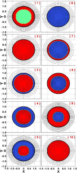
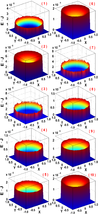
Figure S1: For an oscillating transport current of amplitude $I_{\tt{a}}=I_{c}$, and the temporal steps defined in Fig. 6.1(b) (pag. 6.1), we show the dynamics of the magnetic flux lines (projected isolevels of the vector potential), together with the profiles of current $I_{i}$ across the superconducting wire, in the 1st and 2nd column. Next, 3rd and 4th column show the corresponding evolution of the local density of power dissipation. The profiles of current are displayed according to: red ($+I_{i}$), blue ($-I_{i}$), and green (zero). The plotting interval is $\Delta I_{tr}(t)=I_{\tt{a}}/2$, with t=0 defining the virgin state (i.e., $I_{tr}=0$). Units are $\pi R^{2}J_{c}\equiv{I_{c}}$ for $I_{\rm tr}$, and $(\mu_{0}/4\pi)J_{c}^{2}R^{2}\delta t^{-1}$ for E$\cdotp$J.

As it is well known, the magnetic flux penetrates a superconducting material first entering from the surface towards the center while is shielded by screening currents flowing at the critical value $J_{c}$. Penetration occurs to a depth known as the flux front boundary, where the magnetic flux density drops to zero. Trivially, for long cylindrical wires (length much higher than its radius $R$) with transport current [see Fig. 6.1(a)], the flux front profile may be defined in terms of a set of circular front boundaries tracking the time evolution of the injected transport current. For example, and mainly to illustrate how the patterns of the main electromagnetic quantities evolve along the cyclic process depicted in the Fig. 6.1(b), our numerical results for the local profiles of current $I_{i}$, the components of the magnetic flux density B and the corresponding isolevels of the vector potential A (i.e., the flux lines of B), as well as the local distribution of the density of power dissipation $\textbf{E}\cdot\textbf{J}$ are shown in the section of supplementary material [Figs. S1 & S2 (pags. II, II)]. These figures will be of much help for eventual discussion about the AC hysteretic losses when simultaneous oscillating excitations must to be considered. However, already for this simple case, several aspects have to be noticed.

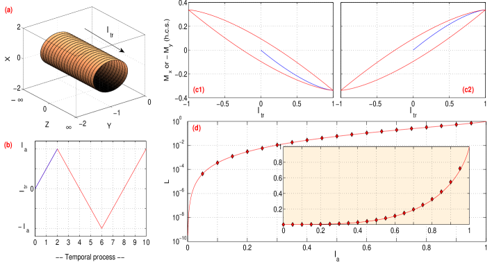
Figure 6.1: For the experimental configuration displayed in subplot (a), and for an injected AC transport current of amplitude $I_{\tt{a}}$ according to the temporal process depicted in subplot (b), we show the calculated components of the magnetic moment for half cross section of the superconducting wire, where (c1) corresponds to $\Omega^{+}$, i.e.: $(x,y)\in\Omega\leavevmode\nobreak\ |\leavevmode\nobreak\ x>0$, and (c2) to $\Omega^{-}$, i.e.: $(x,y)\in\Omega\leavevmode\nobreak\ |\leavevmode\nobreak\ x<0$. Notice that both sections cancel each other to satisfy $\textbf{M}(\Omega)=0$. In subplot (d) we show the calculated hysteretic AC losses per excitation cycle (since time-step 2 to 10). Red solid line corresponds to the exact analytical expression of Eq. (6.14), and solid diamonds corresponds to our numerical results. Inset shows the same results in linear scale. Here and henceforth, units are $\pi R^{2}J_{c}\equiv{I_{c}}$ for $I_{\rm tr}$, $(\mu_{0}/4\pi)J_{c}R$ for B, $J_{c}R^{3}$ for M, and $(\mu_{0}/4\pi)\omega R^{2}J_{c}^{2}$ for the hysteretic losses per cycles of frequency $\omega$.

First of all, let us to focus on the circulating transport currents so as to visualize their contribution to the total magnetic moment of the superconducting sample. Recall that, according to Eq. (6.10), those cases where only transport current is applied, the total magnetization of the superconducting sample becomes zero and the screening currents can be simply called “injected current lines”. They distribute accomplishing the critical state condition $j_{i}=j_{c}$ in the regions where $B(r_{i})\neq 0$. In fact, although these currents produce local patterns of magnetization as it is shown in Fig. 6.1(c), by symmetry, the sum over the whole sample is fully compensated. Nevertheless, for this case, M$(\Omega)=0$ does not imply the absence of hysteretic losses (see Fig. 6.1(d)) which are actually produced by the Joule heat release in those regions where flux transport occurs. On the other hand, as one can see in Fig. S1 (pag. II), the local density of power dissipation ($\textbf{E}\cdot\textbf{J}$) is not uniform despite the material law assumes the critical state condition $j_{i}=j_{c}$. This means that, locally one cannot assume a unique value for the electric field or $E=E_{c}$. In fact, for this case the maximal power dissipation always occurs over the superconducting surface decreasing to zero beyond the flux front.

Eventually, it is worth of mention that for this simple case the current distribution can be reliably calculated by following the boundary flux front defined through axisymmetric circumferences of radius $\tilde{r}=R\sqrt{1-I_{tr}/I_{c}}$, whose section $\tilde{r}<r<R$ produces the intensity of magnetic flux (in polar coordinates):

$$B_{\phi}=\frac{\mu_{0}I_{c}}{2\pi r}\left[\frac{I_{tr}}{I_{c}}+\left(\frac{r^{2}}{R^{2}}-1\right)\right]\,\leavevmode\nobreak\ \,\leavevmode\nobreak\ \,\forall\,\leavevmode\nobreak\ \,\leavevmode\nobreak\ \,\tilde{r}<r<R\,.$$ (6.12)

Notice that here, $I_{tr}$ stands for the applied transport current at a given time, and $I_{c}\equiv J_{c}\pi R^{2}$. Thus, the electric field can be analytically calculated by the one dimensional Maxwell equation $\partial_{r}E_{z}=\partial_{t}B_{\phi}$ satisfying the condition $E_{z}(r<\tilde{r})=0$, i.e.,

$$E_{z}=\frac{\mu_{0}}{2\pi}\ln{\left[\frac{r}{R}\left(1-\frac{I_{tr}}{I_{c}}\right)^{-1/2}\right]}\dot{I}_{tr}\,\leavevmode\nobreak\ \,\leavevmode\nobreak\ \,\forall\,\leavevmode\nobreak\ \,\leavevmode\nobreak\ \,\tilde{r}<r<R\,.$$ (6.13)

In fact, if the temporal evolution of the injected transport current is monotonic the average specific hysteretic loss rate per unit length can be calculated by integration of the local density of power dissipation ($\textbf{E}\cdot\textbf{J}$),

$$\dot{L}_{m}(I_{tr}(t))=\frac{1}{\pi R^{2}}\int_{0}^{2\pi}\int_{\hat{r}}^{R}E_{z}J_{c}\leavevmode\nobreak\ rd\phi dr=-\frac{\mu_{0}}{4\pi^{2}R^{2}}\left[I_{tr}+I_{c}\ln\left(1-\frac{I_{tr}}{I_{c}}\right)\right]\dot{I}_{tr}\,,$$

and integrating it with respect to time, the monotonic hysteretic losses is then

$${L}_{m}(I_{tr}(t))=\frac{\mu_{0}}{4\pi^{2}R^{2}}\left[I_{tr}I_{c}\left(1-\frac{I_{tr}}{2I_{c}}\right)+I_{c}^{2}\left(1-\frac{I_{tr}}{I_{c}}\right)\ln\left(1-\frac{I_{tr}}{I_{c}}\right)\right]$$ (6.14)

Moreover, if $I_{tr}(t)$ is periodic, the dependence of the hysteretic loss density per period on $I_{tr}=I_{\tt{a}}$ ($\tt{a}$ for the amplitude of the oscillating source) remains the same, and therefore the magnitude of the loss per cycle may be straightforwardly obtained from the monotonic first branch as, $L_{f.c.}=4L_{m}$.

6.2.2  Wires under an external AC magnetic flux

With the aim of providing a clear picture of the effects related to the occurrence of local magnetization currents (screening currents produced by external magnetic fields), the second case under consideration will correspond to a superconducting wire under zero transport current condition ($I_{tr}(t)=0$) and subjected to an external magnetic field perpendicular to its surface. Here, we must call readers’ attention to the fact that for this seemingly simple case an exact analytical solution for the dynamics of the flux front profiles has not been reported, although remarkable efforts have been done along the last five decades to implement diverse analytical and numerical approaches [64, 53, 54, 55, 56, 57, 71]. In fact, for an arbitrary relation between the amplitude of the applied field ($H_{a}$) and the full penetration value $H_{p}$, the cyclic hysteretic losses can only be found numerically. Nevertheless, for cylindrical superconducting wires subjected to a monotonic source $H_{0}(t)$, the losses may be approached by the so-called Gurevich’s relation [57]:

$$L_{m}(B_{0}(t))=\dfrac{2B_{p}^{2}}{3\mu_{0}}\left\{\begin{array}[]{ll}\left(\dfrac{B_{0}}{B_{p}}\right)^{3}\left(1-\dfrac{B_{0}}{2B_{p}}\right)\nobreak\leavevmode\nobreak\leavevmode&,\leavevmode\nobreak\ \,\forall\leavevmode\nobreak\ \,\leavevmode\nobreak\ \,B_{0}<B_{p}\\ \\ \dfrac{B_{0}}{B_{p}}-\dfrac{1}{2}\nobreak\leavevmode\nobreak\leavevmode&,\leavevmode\nobreak\ \,\forall\leavevmode\nobreak\ \,\leavevmode\nobreak\ \,B_{0}\geq B_{p}\,\leavevmode\nobreak\ \,\leavevmode\nobreak\ \,.\end{array}\right.$$ (6.18)

Here, the customary relation for superconducting materials $\textbf{B}=\mu_{0}\textbf{H}$ has been assumed, and $B_{p}$ is given by:

$$B_{p}=\frac{2}{\pi}\mu_{0}J_{c}R\,.$$ (6.19)

Just as in the previous case (only transport current), if $B_{0}(t)$ is periodic, the dependence of the hysteretic loss density per period remains the same, and the magnitude of the cyclic losses is higher by a factor of four regarding the monotonic branch.

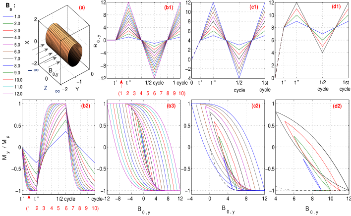
Figure 6.2: For the experimental configuration represented in subplot (a), and before applying an oscillating magnetic flux with amplitude $B_{\tt{a}}=B_{0,y}(t^{\prime\prime})-B_{0,y}(t^{\prime})$, three different initial states $(B_{0,y}(t^{\prime}))$ have been considered. Firstly, a non magnetized wire has been assumed accordingly to the magnetic temporal process displayed in subplot (b1). Subplots (b2) and (b3) show the evolution of the dimensionless magnetic moment $M_{y}/M_{p}$ as a function of the temporal process and the applied magnetic field $B_{0,y}$ respectively. Secondly, a premagnetized sample with $B(t^{\prime})<B_{p}$ has been considered (subplot c1), and the corresponding $M_{y}/M_{p}$ curves are displayed (subplot c2). Thirdly, in (d1) the initial state has been assumed to be $B(t^{\prime})=B_{p}$, and the corresponding $M_{y}/M_{p}$ curves are displayed in (d2). For all plots, curves are labeled according to $B_{\tt{a}}$. In subplots (b1) and (b2) an additional temporal scale in red has been incorporated to allow an straightforward interpretation for the sequence of profiles displayed in the section of supplementary material, Figs. S3 (pag. II) & S4 (pag. II). Recall that units for B are $(\mu_{0}/4\pi)J_{c}R$, and $J_{c}R^{3}$ for M.

( A. ) Features on the magnetic response

For a major understanding of the electromagnetic quantities involved, we have considered the experimental configuration depicted in Fig. 6.2(a) under different amplitudes for the applied magnetic flux $B_{0,y}$. Just for completeness, three different magnetization pre-conditions have been considered as relates the first branch of the temporal processes $t<t^{\prime}$ (see top pane in Fig. 6.2). Thus, subplots (b1) to (b3) correspond to a non magnetized wire for which one gets magnetization loops centered at the coordinates (0,0) of the plane ($M_{y},B_{0,y}$). However, in those cases where $B_{0,y}(t^{\prime})\neq 0$ [Figs. 6.2 (c1) and (d1)] a different behavior reveals. An initial magnetization branch is present when the external AC magnetic flux is switched on ($t=t^{\prime}$) [see dashed lines in Figs. 6.2 (c2) and (d2)]. Then, for $t>t^{\prime}$ the SC wire is subjected to an oscillating magnetic flux of amplitude $B_{\tt{a}}$, such that the first quarter of the subsequent periodic excitation occurs along the interval $t^{\prime}<t<t^{\prime\prime}$, and consequently the AC losses are calculated relative to cycles departing from $t^{\prime\prime}$. For the oscillating process in the above figure, the alternating magnetic field is applied along the same direction of the previous magnetization under the flux conditions $B_{0,y}(t^{\prime})<B_{p}$ and $B_{0,y}\geq B_{p}$ respectively. The following facts have to be noticed:

(i) Concerning to the numerical accuracy, it has to be noticed that the mutual inductance matrices used in this fore, corresponds to the exact analytical solution for filaments of cylindrical cross section. Thus, some discrepancies between the analytical and numerical quantities can be expected. In fact, in the classical results of Ref. [64] it may be noticed that the magnetization curve saturates to a flat value ($M_{p}$) before reaching the analytical limit $B_{p}=8$, which is in agreement with our numerical predictions in Fig. 6.2 ($B_{p}\simeq 7\pm 5\times 10^{-3}$). Accordingly to our numerical method, discrepancies with the analytical solution are explained in geometrical terms. Notice that even for a highly refined mesh, by assuming cylindrical filaments, the entire superconducting area cannot be filled, and therefore some deviation should be expected. We emphasize that other choices for the mesh elements filling the superconducting area could be done, but the complication seems unnecessary if one considers that the accuracy in the obtained physical quantities is already very high, and furthermore this mesh has been recognized to fit well to experimental evidences in the same geometry [65].

(ii) Recalling Eq. (6.10), the sum of the local magnetic moments associated to each of the filaments over the entire superconducting sample increases as $B_{0,y}$ grows monotonically until the condition $B_{0,y}=B_{p}$ is met. Then, the magnetization of the sample saturates to the analytical value $M_{p}=2J_{c}R^{3}/3$ (in our dimensionless units $M_{p}=2/3\approx 0.6667$). Regarding to our numerical results we have obtained $M_{p}\approx 0.655\pm 5\times 10^{-3}$.

(iii) Once the cyclic process starts ($t>t^{\prime\prime}$), and regarding the magnetization loops characterized by AC cycles of external magnetic flux with amplitudes higher than $B_{p}$, the magnetic moment saturates at different values given by the dimensionless relation

$$B_{p^{{\dagger}}}=\mp\left(2B_{p}-B_{\tt{a}}\mp B_{0}(t^{\prime})-1/2\right)\,,$$ (6.20)

where the signs choice is made simultaneously, it for consider the time derivative of the cyclic excitation.

For example, in Fig. 6.2(b3) if $B_{0}(t^{\prime})=0$ and the amplitude of the external magnetic flux is $B_{\tt{a}}=8$, into the cyclic process $(t>t^{\prime\prime})$ the magnetization of the superconducting wire saturates at $B_{0,y}=\mp 5.5$. On the other hand, if the sample has been previously premagnetized, the center of the magnetization loop is displaced in the axis $B_{0,y}$ of the plane $(M_{y},B_{0,y})$ by the amount $B_{0,y}(t^{\prime})$ [see Fig. 6.2 (c2,d2)], and therefore the sample saturates at two different values of the applied magnetic field (e.g., for $B_{\tt{a}}=8$, $M_{y}$ is equals to $M_{p}$ at $B_{0,y}=-1.5$, and $M_{y}$ is equals to $-M_{p}$ at $B_{0,y}=9.5$).

(iv) Remarkably, the set of magnetization loops displayed in Fig. 6.2 serves as a map for any magnetization loop and any arbitrary relation between the experimental parameters $B_{0,y}(t^{\prime})$ and $B_{\tt{a}}$. In fact, it can be done by the simple interpolation of the known shape of the magnetization loops where the first corner of $M_{y}$ (corresponding to the higher excitation peak for the first half of the excitation cycle) always falls over the magnetization branch for $t<t^{\prime\prime}$. Moreover, if $B_{\tt{a}}+B_{t^{\prime}}>B_{p}$ the position of the corners is straightforwardly given by the saturation values $B_{p^{{\dagger}}}$.

( B. ) Flux penetration and local power density

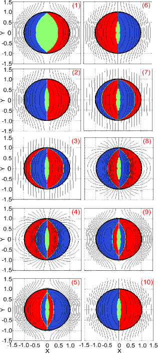
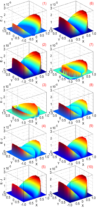
Figure S3: For an external AC magnetic flux applied along the $y-axis$, with amplitude $B_{\tt{a}}=6$, and for the temporal steps defined in Fig. 6.2(b) (pag. 6.2); the 1st and 2nd column show the dynamics of the magnetic flux lines and their corresponding profiles of current $I_{i}$. Next, 3rd and 4th column show the corresponding dynamics of the local density of power dissipation. The profiles of current are displayed according to: red ($+I_{i}$), blue ($-I_{i}$), and green (zero). The plotting interval is $\Delta B_{0,y}=3$, with t=0 defining the virgin state (i.e., $B_{0}=0$). Units are $(\mu_{0}/4\pi)J_{c}R$ for B, and $(\mu_{0}/4\pi)J_{c}^{2}R^{2}\delta t^{-1}$ for E$\cdotp$J.

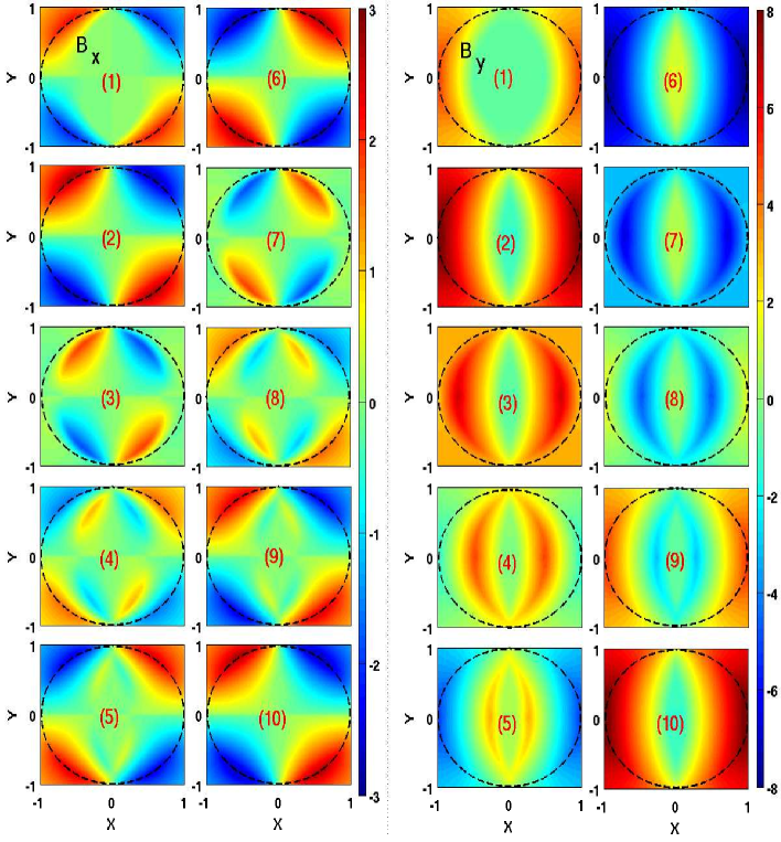
Figure S4: Colormaps for the intensity of the components of magnetic flux density $B_{x}$ (left pane) and $B_{y}$ (right pane) for the square section of area $4R^{2}$ enclosing the cylindrical wire of radius $R=1$. The profiles are plotted in according to the Fig. S3. The superconducting surface is depicted by the black dashed lines. Recall that units for B are $(\mu_{0}/4\pi)J_{c}R$.

For a clear understanding of the different terms affecting the calculation of the hysteretic losses in superconducting wires, it is advisable to get familiar with the local dynamics of the electromagnetic quantities in the same way as it was done in the previous section. Therefore, in the section of supplementary material, readers will find out some of our numerical results for one of the experimental processes depicted in Fig. 6.2. In particular, in Fig. S3 (pag. II) we show the flux penetration profiles for an external AC magnetic flux of amplitude $B_{\tt{a}}=6$ at intervals of $\Delta B_{0,y}=3$, assuming an initially non magnetized wire [see by reference the temporal process depicted in Fig. 6.2(b)]. Also shown are corresponding patterns for the local density of power dissipation across the section of the superconducting wire. The direction of the magnetic field can be tracked from the dynamics of the Cartesian components $B_{x}$ and $B_{y}$ both displayed in Fig. S4 (pag. II).

It becomes clear that the distribution of magnetization currents across the section of the superconducting wire preserves some symmetry respect to both Cartesian axes, although rotational invariance characteristic for transport problems [Fig. S1 (pag. II)] is not fulfilled. Actually, we can argue that for cases with no rotating transverse magnetic field the numerical problem may be reduced to considering only two of the four Cartesian quadrants according to the following symmetry condition: (i) $I_{i}(r_{i}(y^{+})=I_{i}(r_{i}(y^{-})$, being “$y$” the axis of the applied magnetic field $B_{0}$. Moreover, for our current case also the symmetry condition (ii) $I_{i}(r_{i}(x^{+})=-I_{i}(r_{i}(x^{-})$, being $x$ the axis perpendicular to the direction of $B_{0}$ may be called. However, the latter can only be fulfilled as long as the transport current condition $I_{tr}=0$ occurs.

As it may be observed in Fig. S3 (pag. II), once the external magnetic flux $B_{0,y}$ is switched on, a set of screening currents symmetric along the $y$-axis but antisymmetric by sign along the $x-$axis appears so as to expell the magnetic field from the inner sample [see also Fig. S4 (pag. II)]. Actually, for transverse magnetic fields, it is the Faraday’s law which produces the simultaneous occurrence of positive and negative screening currents distributed along the positive and negative semi-axis, but both orthonormal to the direction of the applied magnetic field. Thus, if the rate $\Delta B_{0,y}(t)$ is monotonic, the shape of the flux free region approaches to ellipses with their foci along the $y-$axis, but with acute nodes in the boundaries of their major axis. Moreover, the associated lengths to the major and minor semi-axis of the ellipse also change responding to the variation of the external magnetic flux in the different points where the screening currents are allocated, which is in concordance with Refs. [64, 67, 68, 69, 70, 71, 81].

As regards the local power loss density [right pane in Fig. S3 (pag. II)], we have observed some fine structure details which are worth of mention. First, if the rate of magnetic flux $\Delta B_{0,y}$ is monotonic (without change of sign), it is to be noticed that the specific local power density preserves the same kind of pattern observed for the dynamics of the local profiles of the magnetic flux density component $B_{y,i}$. However, the role played by the orthonormal component $B_{x,i}$ is rather different and geometry dependent [see subplots (1) and (2) in Figs. S3 (pag. II) & S4 (pag. II)]. Then, as soon as $\Delta B_{0,y}$ changes sign, the local distribution of power density is much more complex as the core enclosed by the flux fronts satisfying the condition $E=0$ must be shielded [see the sequence of subplots (3) to (10) in Figs. S3 (pag. II) & S4 (pag. II)].

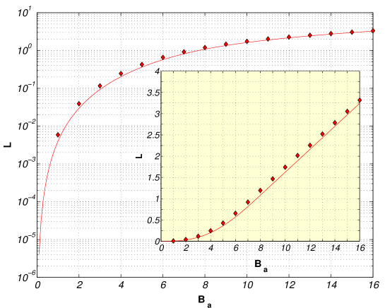
Figure 6.3: Hysteretic AC losses per cycle for an oscillating magnetic field of amplitude $B_{\tt{a}}$. Red solid line corresponds to the analytical approach of Eq. (6.18), and diamonds correspond to our numerical calculations. Inset shows the same results in linear scale. Units are $(\mu_{0}/4\pi)J_{c}R$ for $B_{0,y}$, and $(\mu_{0}/4\pi)\omega R^{2}J_{c}^{2}$ for the hysteretic losses per cycles of frequency $\omega$.

In general, power losses appear for the whole section where the magnetization currents are displayed, but their maximum contribution always occurs over the external surface of the superconducting sample. On the other hand, for the hysteretic losses per cycle the total amount of heat release can be straightforwardly calculated based on energy transport over the external surface of the superconducting sample as explained below.

6.2.3  Ultimate considerations on the AC losses

At this point and after gaining some experience by the analysis of wires under transport or applied magnetic field, we are in the position of casting Eq. (6.11) in different forms for convenient interpretation of the AC losses. Thus, taking advantage of the knowledge generated in the above sections, below we reformulate the argument $\dot{L}$ of Eq. (6.11) in terms of the definitions for E or J. This will allow a physical interpretation of the mechanism responsible for AC losses in complex configurations.

( A. ) Conventional approach [B-oriented]

First of all, recalling that the electric field may be defined for discretized time layers as $\textbf{E}=-\Delta\textbf{A}/\Delta t$, and furthermore, that it can be computed from the sum of the external vector potential $\textbf{A}_{0}(\textbf{B}_{0})$ [see Eq. (6.8)] and the vector potential induced by the screening currents $\textbf{A}_{ind}(\textbf{J}(r_{i}))$ [see Eqs. (6.1) & (6.2)], the losses of power density $\dot{L}\equiv\Delta L/\Delta t$ may be rewritten as

$$\Delta L=-\int_{\Omega}\Delta\textbf{A}_{0}\cdot\textbf{J}\leavevmode\nobreak\ dr-\int_{\Omega}\Delta\textbf{A}_{ind}\cdot\textbf{J}\leavevmode\nobreak\ dr\,.$$ (6.21)

Thus, recalling Eq. (6.10), the first term on the right-hand side of Eq. (6.21) becomes

$$\Delta L_{0}(\Delta B_{0,y})=-\int_{\Omega}\Delta\textbf{A}_{0}\cdot J\leavevmode\nobreak\ dr\equiv\int_{\Omega}M_{y}\leavevmode\nobreak\ dB_{0,y}\,,$$ (6.22)

which corresponds to the losses produced by an external excitation of magnetic flux density $B_{0}(t)$.

In fact, since the work by Ashkin (Ref. [64]), it is well known that for screening currents produced by external variations of an applied magnetic field of flux density $B_{0,y}$, the so called magnetization currents, the average AC losses can be straightforwardly calculated as the enclosed area by the magnetization loop $M_{y}$ as a function of the excitation $B_{0,y}$ (Fig. 6.2). Thus, as long as the experimental configuration is such that $I_{tr}(t)=0$, physically the AC hysteretic losses may be understood as surface losses due to remagnetization.

Nevertheless, as in most applications of superconducting wires, the system is subjected to a simultaneous oscillating transport current, a most careful analysis of the second term at the right-hand side of Eq. (6.21) is needed.

First recall that in the CS theory the MQS approach allows us to define Ampere’s law as the spatial condition $\mu_{0}\nabla\times\textbf{B}=\textbf{J}$, where $\textbf{B}_{i}$ is the local density of magnetic flux produced by the induced screening currents of density $\textbf{J}(\textbf{r}_{i})$ plus the density of magnetic flux produced by the external excitation $\textbf{B}_{0}(\textbf{r}_{i})$, i.e., $\textbf{B}_{i}=\textbf{B}_{0}(\textbf{r}_{i})+\textbf{B}_{ind}(\textbf{r}_{ij})$, so that the second term at the right-hand side of Eq. (6.21) may be rewritten as

$$\Delta L_{ind}=-\mu_{0}\int_{\Omega}\Delta\textbf{A}_{ind}\cdot\nabla\times\left(\textbf{B}_{0}+\textbf{B}_{ind}\right)\leavevmode\nobreak\ dr\,.$$ (6.23)

On the other hand, accordingly to the CS statement, $\Delta{J_{i}}=\pm J_{c}\neq 0$ accomplishes for the flux front profile, ergo $\Delta\textbf{A}_{ind}\equiv{\rm M}_{ij}\Delta J_{i}\neq 0$. Then, for systems only subjected to external magnetic fields, the distribution of screening currents over the cross section of the superconducting sample is such that the induced magnetic field over flux front is rotationally invariant with respect to the direction of the applied magnetic field. For example, considering the first monotonic branch in cases of Fig. 6.2, the flux front profile is defined by $B_{ind}(t)=-B_{0,y}(t)$. Said in other words, the induced magnetic field flows only in opposite direction to $B_{0}$ so that $\Delta L_{ind}=0$ as long as $I_{tr}(t)\equiv 0$, and therefore the hysteretic losses may be straightforwardly computed as $\Delta L\equiv\Delta L_{0}$ in the fashion of Eq. (6.22). Nevertheless, if $I_{tr}(t)\neq 0$ the local density of magnetic flux is not rotationally invariant with respect to the components of the induced magnetic field. For example, for the cases described in the previous subchapter (Fig. 6.1), where $B_{0,y}(t)\equiv 0$ (absence of magnetization currents), the magnetic flux density produced by the screening currents $J_{i}$, so called there injected current lines, shows two components $B_{x,i}$ and $B_{y,i}$ so that $\nabla\times\textbf{B}_{i}\neq 0$, and thence that $\Delta L\equiv\Delta L_{ind}\neq 0$ despite $\int_{\Omega}M(\textbf{r}_{i})\equiv 0$.

In order to understand the underlying physics behind the the concept of injected current lines into the critical state theory, at least for the 2D configurations studied along this chapter, it becomes useful to further analyze Eq. (6.23) by the vectorial definition $\textbf{A}\cdot\nabla\times\textbf{B}=$ $\nabla\cdot\textbf{B}\times\textbf{A}+$ $\textbf{B}\cdot\nabla\times\textbf{A}$, such that we can write

$$\Delta L_{ind}=-\mu_{0}\int_{\Omega}\nabla\cdot(\textbf{B}\times\Delta\textbf{A}_{ind})\leavevmode\nobreak\ dr-\mu_{0}\int_{\Omega}\frac{\textbf{B}\cdot\Delta\textbf{B}}{2}\leavevmode\nobreak\ dr\,.$$ (6.24)

Into this framework the first integral turns to a surface integral over the curved walls of the cylinder, which does not contribute to the average losses because the contribution to the surface integral from the end planes vanishes as $\textbf{B}\times\textbf{A}_{ind}\cdot\hat{\textbf{z}}=0$, while the integral over the lateral surface turns zero in a closed cycle. Therefore, the contribution of the injected current lines may be understood by the simple relation

$$\Delta L_{ind}=-\mu_{0}\int_{\Omega}\frac{\textbf{B}\cdot\Delta\textbf{B}}{2}\leavevmode\nobreak\ dr\,,$$ (6.25)

where it is pointed out that significant reductions of the hysteretic losses may be achieved by reducing the magnitude of the local inductive magnetic field.

( B. ) Alternative approach [S-oriented]

In order to justify that the hysteretic losses may be calculated by the knowledge of the electromagnetic quantities over the external surface of a superconducting material, it is interesting to transform Eq. (6.11) in terms of a second formulation based upon the definition of J instead of E. Indeed, assuredly the specific losses can be evaluated by the conservation energy principle defining $\textbf{J}=\nabla\times\textbf{H}-\partial_{t}\textbf{D}$ and by using the divergence theorem as follows:

$$\dot{L}=\int_{\Phi}\textbf{E}\cdot\left(\nabla\times\textbf{H}-\partial_{t}\textbf{D}\right)dr=-\int_{\Phi}(\textbf{E}\cdot\partial_{t}\textbf{D}+\textbf{H}\cdot\partial_{t}\textbf{B})\leavevmode\nobreak\ dr-\oint_{s}\textbf{S}\cdot\hat{\textbf{n}}\leavevmode\nobreak\ ds\,,$$

where $\Phi$ is introduced to distinguish the volume integral over the entire superconducting sample from the surface integral over the flux fronts defined by the Poynting’s vector $\textbf{S}=\textbf{E}\times\textbf{H}$, and $\hat{\textbf{n}}$ the unit vector normal to its surface element $(d\hat{\textbf{s}}_{i}=ds\hat{\textbf{n}})$.

The first term on the right-hand side of Eq. (6) represents the total electromagnetic energy stored within the superconductor volume, and the second one corresponds to the energy flow produced by the local variations of magnetic field as a consequence of the occurrence of screening currents. Then, if one is only interested on the hysteretic losses per closed cycles, one is entitled to evaluate the AC losses between two well-defined stationary regimes,

$$L=-\omega\int_{peak\leavevmode\nobreak\ a}^{peak\leavevmode\nobreak\ b}dt\oint_{s}\textbf{S}\cdot\hat{\textbf{n}}\leavevmode\nobreak\ ds=-2\omega\int_{h.f}dt\oint_{s}\textbf{S}\cdot\hat{\textbf{n}}\leavevmode\nobreak\ ds\,,$$ (6.27)

because the total electromagnetic energy is a conserved quantity between two consecutive peaks defined by the wavelength of the oscillating source. In fact, the calculation can be simplified following the same argument to consider only half cycle ($h.f$) of the excitation process. Remarkably, this fact can be straightforwardly observed by comparison between the local profiles $\textbf{E}\cdot\textbf{J}$ for the excitations of Figs. 6.1(a) or 6.2(b1), accordingly to the steps (6) and (10) in Figs. S1 (pag. II) and S3 (pag. II), respectively.

Finally, taking advantage of the two dimensional symmetry of our problem (as we have assumed wires of infinite length), Eq. (6.24) may be transformed to a path integral for the flux of energy over the external surface of the superconducting wire, which for cylindrical wires in polar coordinates is equivalent to say that the hysteretic losses per unit length can be reliably calculated by the following expression:

$$L=-2\omega\int_{h.f}dt\oint_{l}\textbf{S}\cdot d\hat{\textbf{{l}}}=\left.-2\omega R\int_{h.f}dt\oint_{l}\textbf{S}\cdot\hat{\textbf{r}}\leavevmode\nobreak\ d\phi\leavevmode\nobreak\ \right|_{r=R}\,.$$ (6.28)

  6.3 SC wires under simultaneous AC excitations $(\textbf{B}_{0}$ , $I_{tr})$

As we have mentioned before, the implementation of superconducting wire technology straightforwardly depends on the demonstration of their reliability, competitive advantages in terms of improved efficiency and reduced operating costs, with capital costs comparable to those of conventional devices. Thus, for the development of competitive devices for the industry, it is important to precisely understand the AC loss properties when realistic non-trivial AC excitations have to be considered. In fact, almost in all the conceived applications for superconducting wires, is well known that each one of the wires holds an AC transport current and experiences an additional AC magnetic field due to the neighboring wires. This situation is found, for example, in superconductor windings for AC magnets, generators, transformers and motors, where each turn feels the magnetic field of all the others [82, 83, 84, 85, 86, 87].

The first conceptualization of the problem of superconducting wires under configurations of simultaneous alternating current and applied magnetic field was provided in 1966 by Hancox [52], who studied the AC losses through simplified analytical methods for determining the flux front profile in an infinite slab subjected to a field applied parallel to the direction of the injected transport current. This work went almost unnoticed for over a decade, until a similar approach was proposed in 1979 by Carr [88]. Then, the same kind of experimental configurations but for monotonic rates of the experimental sources $(B_{0},I_{tr})$ has been studied since the 1990’s, under the assumptions of very thin superconducting strips to allow different analytical considerations [61, 62, 89]. However, in more realistic situations, where the cross section of the superconducting sample cannot be reduced one dimension, the use of exact analytical methods is not feasible. Thus, the use of numerical methods as the described in previous sections becomes in the more attainable procedure for the forecast and understanding of the electromagnetic observables such as the magnetization curves and the AC power density losses.

It is worth mentioning that despite the fact that there is a significant number of works assuming isolated superconducting wires of diverse geometries, mainly strips subjected to synchronous excitations [88, 90, 91, 92, 73, 89, 93, 75, 94, 95, 96, 97, 98, 99, 100, 101, 102, 103, 104, 105, 106], a thoroughly study of cylindrical superconducting wires was still absent, and therefore some outstanding predictions had not been reported before [50].

In the present subchapter, we show a comprehensive study of the physical features associated to the local electrodynamics of superconducting wires under the combined action of AC current and AC magnetic field, which continues our previous discussion and constitutes a step forward in the understanding of the electromagnetic observables and the local effects associated to the AC losses. Section 6.3.1 is restricted to the situation of a synchronous AC excitation $(B_{0},I_{tr})$, corresponding to uniform AC magnetic field $B_{0,y}$ in phase with the injected transport current $I_{tr}$, both with the same oscillating frequency (see Fig. 6.4). Also, synchronous excitations are considered in situations where the superconducting wire has been premagnetized (see Fig. 6.9, pag. 6.9). On the other hand, section 6.3.2 addresses the effects related to the consideration of asynchronous excitations, in which, both sources may be out of phase and apply at different frequencies (see Fig. 6.12, pag. 6.12). Premagnetized wires subjected to synchronous or asynchronous sources, may be found in superconducting multicoils for the production of high magnetic fields [107], accelerator magnet technologies [107, 108, 109], and superconducting magnetic energy storage systems [110].

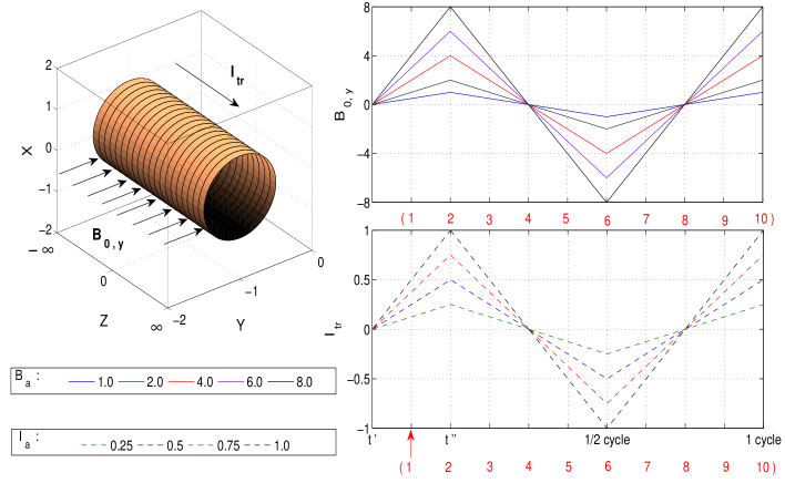
Figure 6.4: Sketch of some of the experimental processes analyzed along this chapter. Here, cylindrical SC wires subjected to synchronous oscillating excitations $B_{0,y}$ and $I_{tr}$, of amplitudes $B_{\tt{a}}$ and $I_{\tt{a}}$ have been considered,

6.3.1  Synchronous excitations

Accordingly to the cases explored in previous sections and holding the aim of achieving a clearest understanding of the electromagnetic quantities involved in the actual use of superconducting wires, is continued by our discussion considering the experimental scenario displayed in Fig. 6.4.

( A. ) Flux penetration profiles

Certainly, the flux front profile in the initial stage penetrates from the surface as the intensity of the external excitations ($B_{0,y}$,$I_{tr}$) increases (see Figs. 6.5 & 6.6). Recall that screening currents produced by the external excitations have been conveniently introduced in terms of two different groups depending on the nature of the source. On the one hand, we speak about magnetization currents produced by the excitation magnetic flux density $B_{0,y}$, and on the other hand, we refer to the injected current lines which must accomplish the additional global constraint $\sum_{i}{I}_{i}(t)\equiv{I}_{tr}(t)$ [Eq. (6.9)]. When the action of isolated sources is conceived, the distribution of screening currents preserves a well defined symmetry. However, for simultaneous application of both sources (Fig. 6.4), the consumption of the magnetization currents by the injected current lines distorts the axisymmetric orientation of the flux-front, by displacing the current free core to the left during the monotonic branch (Figs. 6.5 & 6.6).

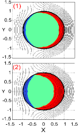
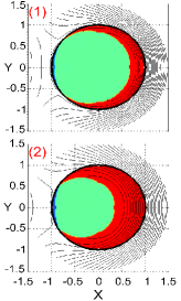
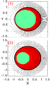
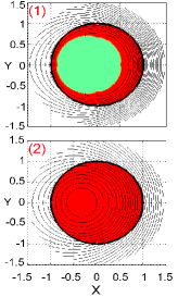
Figure 6.5: Evolution of the magnetic flux lines and their corresponding profiles of current with simultaneous oscillating sources $(B_{0,y},I_{tr})$ of amplitudes $B_{\tt{a}}=2$ (low field) and, 1st column: $I_{\tt{a}}=0.25$, 2nd column: $I_{\tt{a}}=0.5$, 3rd column: $I_{\tt{a}}=0.75$, and 4th column: $I_{\tt{a}}=1$. Subplots are labeled according to the monotonic branch of the experimental processes depicted in Fig. 6.4. For the branches corresponding to the synchronous cyclic excitation see Fig. S5 (pag. II).

For low magnetic fields (Fig. 6.5), the profiles of current density are rather similar to those obtained for $B_{0,y}=0$. The basic difference is that the center of the current free core moves towards the semiaxis $x$-negative. In fact, if the intensity of the transport current is high enough, the flux front becomes nearly circular (current-like). Then, the distribution of screening currents may be understood as the straightforward overlapping of the profiles of current density for isolated sources $I_{tr}$ [Fig. S1 (pag. II)] and $B_{0,y}$ [Fig. S3 (pag. II)], and additionally displacing the center of the core devoid of electric current and magnetic flux (green zone) by the respective difference between the known flux fronts. It should be mentioned that such assumption has been made in Refs. [61] & [62] for calculating the current profiles for thin strips with synchronous excitations $(B_{0},I_{tr})$. Nevertheless, recently it has been proved that even in this simple configuration, the overlapping principle for the flux front tracking may be only fulfilled for high current and low applied field [102].

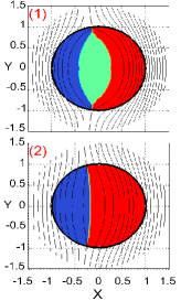
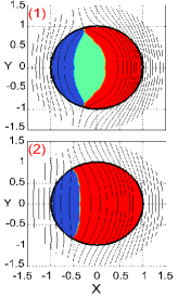
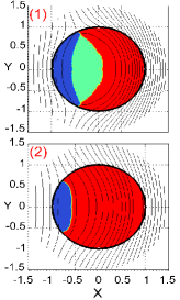
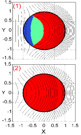
Figure 6.6: Evolution of the magnetic flux lines (projected isolevels of the vector potential) and their corresponding profiles of current with simultaneous oscillating sources $(B_{0,y},I_{tr})$ of amplitudes $B_{\tt{a}}=8$ (high field) and, 1st column: $I_{\tt{a}}=0.25$, 2nd column: $I_{\tt{a}}=0.5$, 3rd column: $I_{\tt{a}}=0.75$, and 4th column: $I_{\tt{a}}=1$. Subplots are labeled according to the monotonic branch of the experimental processes depicted in Fig. 6.4, i.e., label (1) identifies the time-step corresponding to half of the first branch, and (2) the first excitation peak. For visualizing the electromagnetic response in the following branches (cyclic response) reader is advised to see Fig. S8 (pag. II).

Likewise, if the applied magnetic field is intense enough as compared to the transport current (see e.g., left side in Fig. 6.6) the distribution of screening currents is field-like. Nevertheless, the inherent existence of injected current lines makes it impossible to discern which filaments correspond to the so called magnetization currents, and which are the injected current lines. Certainly, for the monotonic branch of the cyclic excitation and before attaining a full penetration state by the screening currents, the “active” zone (blue) where $I_{i}$ takes the value $-I_{c}$ straightforwardly corresponds to the so called magnetization currents. However, the remaining “active” zone (red) defined by screening currents $I_{i}$ taking the value $I_{c}$ is not spatially symmetric as regards the direction of the applied magnetic field, which means that a certain amount of the magnetization currents are contributing in the same direction as the transport current, whilst another part has been consumed by the injected current lines. As it will be shown below, a parallel effect is that the density of magnetic flux increases in the “active” zone, where the patterns of injected current lines dominate.

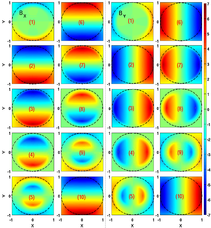
Figure S2: Colormaps for the intensity of the components of magnetic flux density $B_{x}$ (left pane) and $B_{y}$ (right pane) for the square section of area $4R^{2}$ enclosing the cylindrical wire of radius $R=1$. The profiles are plotted in according to Fig. S1, and the superconducting surface is depicted by black dashed lines. Units are $(\mu_{0}/4\pi)J_{c}R$ for B.

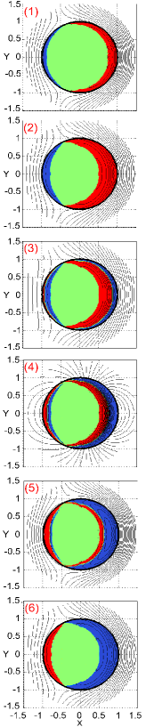
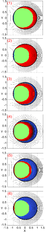
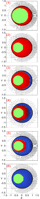
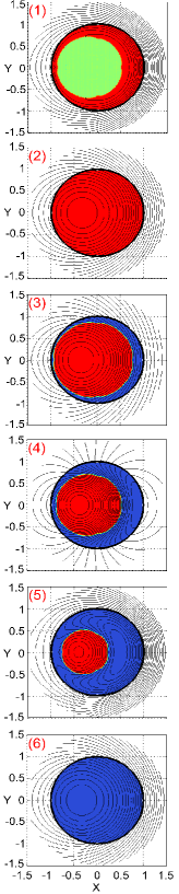
Figure S5: Evolution of the magnetic flux lines and profiles of current with simultaneous oscillating sources $B_{0,y}$ and $I_{tr}$, of amplitudes $B_{\tt{a}}=2$ (low field) and: $I_{\tt{a}}=0.25$ (1st column), $I_{\tt{a}}=0.5$ (2nd column), $I_{\tt{a}}=0.75$ (3rd column), and $I_{\tt{a}}=1$ (4th column). Plotting interval is $(B_{\tt{a}}/2,I_{\tt{a}}/2)$, where the time-step (1) defines the condition $(1,I_{\tt{a}}/2)$ [see also Fig. 6.4 (pag. 6.4)]. By symmetry, only the first half of the AC cycle is shown [i.e., time-steps (2) to (6)].

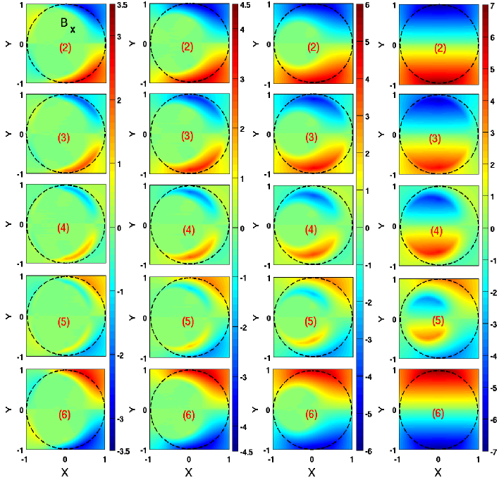
Figure S6: Colormaps for the evolution of the component of magnetic flux density $B_{x}$, corresponding to the current profiles displayed in Fig. S5.

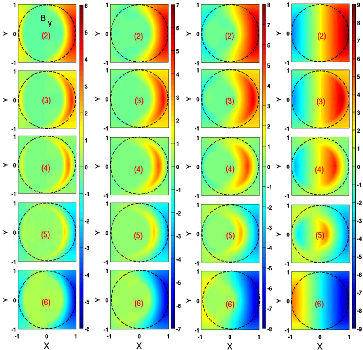
Figure S7: Colormaps for the evolution of the component of magnetic flux density $B_{y}$, corresponding to the current profiles displayed in Fig. S5.

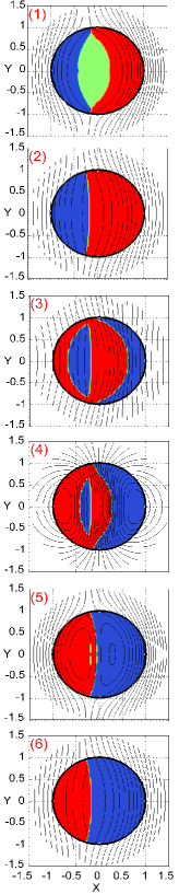
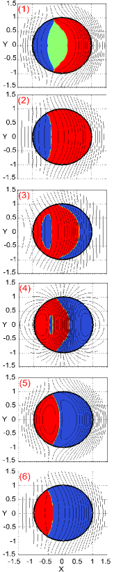
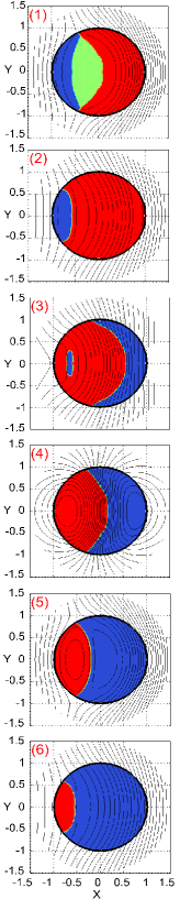
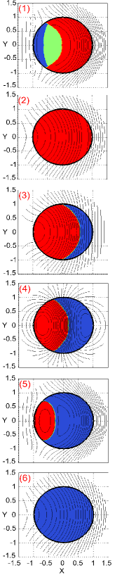
Figure S8: Evolution of the magnetic flux lines and profiles of current with synchronous oscillating sources $(B_{0,y},I_{tr})$ of amplitudes $B_{\tt{a}}=8$ (high field) and, $I_{\tt{a}}=0.25$ (1st column), $I_{\tt{a}}=0.5$ (2nd column), $I_{\tt{a}}=0.75$ (3rd column), and $I_{\tt{a}}=1$ (4th column). Plotting interval is $(B_{\tt{a}}/2,I_{\tt{a}}/2)$, where the time step (1) defines the condition $(8,I_{\tt{a}}/2)$ [see also Fig. 6.4 (pag. 6.4)].

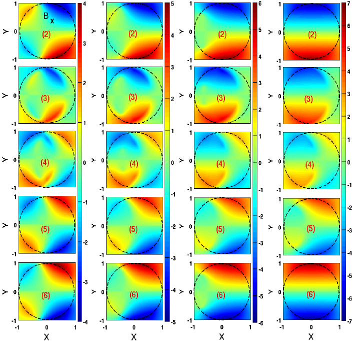
Figure S9: Colormaps for the evolution of the component of magnetic flux density $B_{x}$, corresponding to the current profiles displayed in Fig. S8.

For the cyclic processes displayed in Fig. 6.4 tracking the flux front for synchronous excitation with low magnetic field is intuitive [Fig. S5 (pag. II)], although following up the components of the magnetic flux density $B_{x}$ [Fig. S6 (pag. II)] and $B_{y}$ [Fig. S7 (pag. II)] is not. For high magnetic fields, ascertaining the distribution of screening currents in the cyclic stage is much more elaborated, as long as the electromagnetic history is not erased by the maximal condition for the amplitude of the AC transport current $I_{\tt{a}}=I_{c}$. Actually, if $I_{\tt{a}}<I_{c}$ the flux fronts do not overlap to a unique contour line defined by the filaments with current alternating between $I_{c}$ and $-I_{c}$ [Fig. S8 (pag. II)]. Likewise, describing the evolution of the magnetic flux density [Figs. S9-S10 (pags. II-II)] is also complicated if one compares them with the simplest cases in which isolated sources are assumed [Fig. S2 (pag. II) & Fig. S4 (pag. II)].

Although the analysis of the magnetic flux density $B$ is complicated, one of the most outstanding observations for considering synchronous excitations as shown in Fig. 6.4, is that the local distribution of magnetic field preserves the same kind of pattern along the cyclic stage, independently of the intensity of the external sources. Thus, one can notice that the maximal density of magnetic flux occurs always to the right side of the superconducting wire, which corresponds to the “active” zone where the injected current lines are dominating the system. Concomitantly, substantial distortions of the magnetic flux density outside the wire appear. These are particularly marked when $B_{0,y}$ and $I_{tr}$ tend to zero during the excitation.

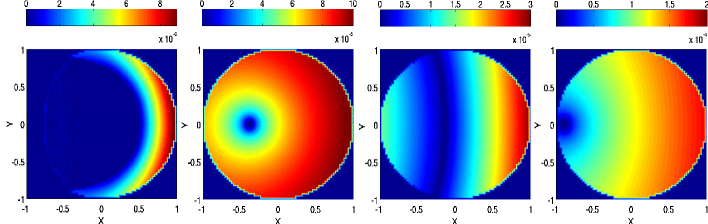
Figure 6.7: Local density of power dissipation E$\cdotp$J at the time frame of full cycle (step number 10 in Fig. 6.4) for synchronous oscillating sources of amplitudes: (1st pane) $B_{\tt{a}}=8$ and $I_{\tt{a}}=0.25$, (2nd pane) $B_{\tt{a}}=8$ and $I_{\tt{a}}=1.0$, (3rd pane) $B_{\tt{a}}=2$ and $I_{\tt{a}}=0.25$, (4th pane) $B_{\tt{a}}=2$ and $I_{\tt{a}}=1.0$. The local dynamics for the aforementioned quantities in the full cyclic process including the initial monotonic branch, can be inferred from the supplementary figures for the low-field regime [Fig. S14 (pag. II)], and the high-field regime [Fig. S15 (pag. II)].

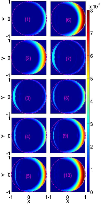
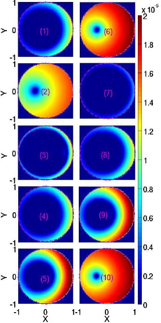
Figure S14: Evolution of the local density of power dissipation E$\cdotp$J for oscillating sources of amplitude $B_{\tt{a}}=2$ and: $I_{\tt{a}}=0.25$ (left pane), and $I_{\tt{a}}=1$ (right pane). Each step has been plotted according to the temporal process depicted in Fig. 6.4. In the right pane, the colormap for subplots (2), (6), and (10) have to be renormalized by a factor of 5. Also, some of the corresponding flux profiles have been displayed in the left and right columns of Figs. S5- S7.

Remarkably, the strong localization of the inner density of magnetic flux density produces a significant change in the local distribution of density of power dissipation $\textbf{E}\cdot\textbf{J}$, which rises from low-value parts (blue) to high-value parts (red) [see, Fig. 6.7], in such manner that the heat release from the superconducting wire is highly localized too. In fact, this asymmetric distribution of power losses regarding the perpendicular direction to the orientation of B, remains along the entire cyclic process as long as both excitations evolve synchronous [see e.g., Figs. S14-S16 (pags. II-II)]. Therefore, its pronounced bias unfolding across the wire could increase the probability of quench.

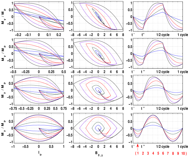
Figure 6.8: The dimensionless magnetic moment $M_{y}/M_{p}$ for the synchronous AC excitations displayed in Fig. 6.4. Curves are shown as function of the injected transport current $I_{tr}$ (left pane), the applied magnetic field $B_{0,y}$ (central pane), or either by its temporal evolution (right pane). In this figure, the amplitudes for the electromagnetic AC sources can be extracted either from color comparison with curves in Fig. 6.4, or from the respective limits along the abscissas in left and right panes.

( B. ) Magnetic response

The above described behavior for the local flux distributions gives way to the following features on the magnetic moment response.

For the set of cases displayed in Fig. 6.4, we have analyzed the dynamics of the magnetic moment component $M_{y}$ as a function of the amplitudes of the electromagnetic sources $B_{\tt{a}}$ and $I_{\tt{a}}$ (Fig. 6.8). Results are shown accordingly to the temporal dependence with the synchronous AC excitations (right pane), and also by their dependence with each one of the electromagnetic sources, say $I_{tr}$ (left pane) and $B_{0,y}$ (middle pane). We realize that only for small values of the amplitude of the ac transport current, almost Bean-like loops of $M_{y}$ obtain. However, as $I_{\tt{a}}$ grows we notice a progressive disappearance of the flat saturation behavior for values of $B_{\tt{a}}$ higher than $B_{p}$. Actually, the notorious change of sign for the slope of the magnetic moment curve along a monotonic branch of the synchronous AC excitation, allows an unambiguous glimpse of the consumption of magnetization lines by effect of injected current lines. Remarkably, this phenomenon ends up with a symmetrization of the loops, both as functions of $B_{y}$ and $I_{tr}$, into characteristic lenticular shapes. As a consequence of this process, a distinct low-pass filtering effect comes to the fore which, in the case of the triangular input excitations considered here, yields a nearly perfect sinusoidal (first-harmonic) output signal $M_{y}(t)$.

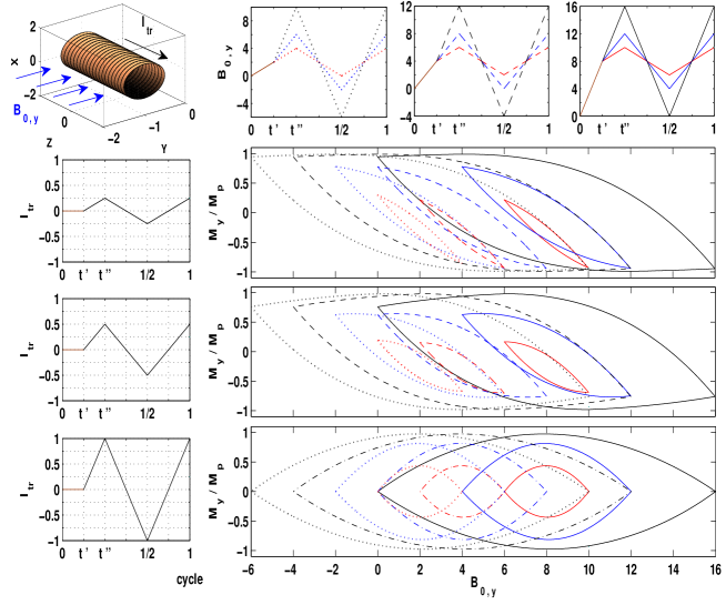
Figure 6.9: Dimensionless magnetic moment $M_{y}/M_{p}$ as a function of the applied magnetic field $B_{0,y}$ for cycles of simultaneous ac excitations $B_{0,y}$ and $I_{tr}$ of amplitudes $(B_{\tt{a}},I_{\tt{a}})$. Although the excitation peak to peak of both sources assumes synchronous and with equal frequency, several premagnetized samples have been considered according to: $B(t^{\prime})=2$, $B(t^{\prime})=4$ and $B(t^{\prime})=8$ (see 1st row), for the time instant when the ac current $I_{tr}(t^{\prime})$ is switched on. Regarding to the cyclic process (i.e, from $t^{\prime\prime}$ to 1), several cases are shown accordingly to the amplitudes $I_{tr}(t^{\prime\prime})=0.25$ (see 2nd row), $I_{tr}(t^{\prime\prime})=0.5$ (see 3rd row), and $I_{tr}(t^{\prime\prime})=1$ (see 4th row), as well as to $B_{\tt{a}}=$2 (dotted lines), $B_{\tt{a}}=$4 (dashed lines) and $B_{\tt{a}}=$8 (straight lines) respectively.

Interestingly, from the cycles of $M_{y}$, it furthermore appears that a proper determination of the “active” zones depends on the history of the virgin branch, thus bearing witness to the system’s memory. For example, a positive slope in the synchronous excitation $B_{y}$ and $I_{tr}$ produces a higher power dissipation in the positive $x$-direction perpendicular to the wire. On the other side, if the superconducting wire has been premagnetized before switching on the synchronous AC excitation [$t=t^{\prime}$ at Fig. 6.9], the magnetic moment curve is displaced in such a manner that the center of the magnetization loop lies over the master curve for the isolated excitation $B_{0,y}$ at $M_{y}(t^{\prime})$ (see Fig. 6.2), and the nodes move towards the boundaries $B_{0,y}(t^{\prime})\pm B_{\tt{a}}$.

( C. ) AC Losses

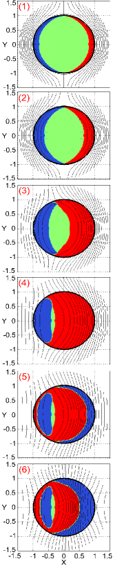
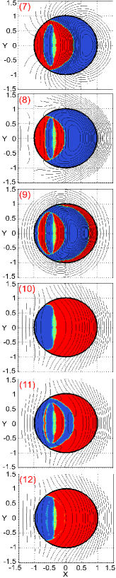
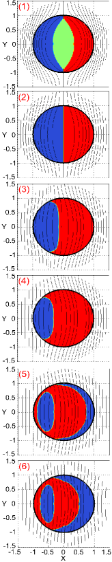
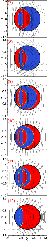
Figure S11: Evolution of the magnetic flux lines and profiles of current with synchronous oscillating sources $B_{0,y}$ and $I_{tr}$ of amplitudes $B_{\tt{a}}=4$ (intermediate field) and $I_{\tt{a}}=0.5$. Results for two premagnetized samples with $B(t^{\prime})=2$ (left pane) and $B(t^{\prime})=8$ (right pane) are shown. Numeric tags in the upper left corner of each subplot have been incorporated according to the following time-steps for the experimental process depicted in Fig. 6.9: (1) corresponds to half of the time between $t=0$ and $t=t^{\prime}$, then (2) at $t=t^{\prime}$, and for (2) to (12) increases of $\Delta t\equiv 1/8$ per unit cycle have been considered. Thus, the full cycle peak-to-peak corresponds to the subplots (4) to (12), respectively.

Regarding the power density losses attained along the premagnetization process, it does not seem to play any role in the calculation of the AC losses (Fig. 6.10). At least, this was observed to the precision of our calculations. However, the definition of the flux front profile becomes much more tangled, because multiple domains enclosed by contour lines defined by the screening currents alternating from $I_{c}$ to $-I_{c}$ arise [see Fig. S11 (pag. II)].

Notwithstanding, the Bean-like magnetic moment curves as the described above, and the ostensible explanation for the distribution of screening currents in terms of the consumption of magnetization lines by the injected current lines, is actually insufficient for the proper interpretation of the actual AC losses produced by synchronous excitations. In fact, despite the collection of reliable experimental data is quite laborious (because there are many pitfalls in the measurement procedures), there is an extended consensus that the heat release by the superconducting wire may come from the electromagnetic sources $B_{0}$ and $I_{tr}$ in independent manners [101, 93, 95, 96]. Moreover, many works dealing with this issue argue that the transport loss and the magnetization loss can be separately determined by electromagnetic measurements at least for low values of the magnetic field and high currents or vice versa [111, 112, 113, 114, 115]. However, as we have discussed before, for general cases, the competence between the magnetization currents and the injected current lines involving axisymmetric distributions of the screening currents, generates a strong localization of the local density of magnetic flux, as well as of the local density of power losses, which makes it difficult discriminating the role of the AC losses introduced by the inductive terms [Eq. (6.25)]. Therefore, from the theoretical point of view, it is advisable using experimental methods based upon the S-oriented approach (pag. 6), such as calorimetric methods which directly make a measurement of the release flux of energy over the superconducting surface [99, 100, 116, 117, 118].

As we will show below, the feasibility of approaching the total AC loss by overlapping the isolated contributions, strongly depends on the relative magnitudes of the AC field $B_{0}$, and the AC transport current $I_{tr}$. Accordingly to the numerical experiments shown in Figs. 6.4 & 6.9, eventually, we will present a percentage analysis of the actual AC loss for synchronous excitations, $L(B_{\tt{a}},I_{\tt{a}})$, in comparison with the most celebrated approaches. Our numerical results for $L(B_{\tt{a}},I_{\tt{a}})$ are displayed in Fig. 6.10 both in logarithmic and linear -scales with the aim of remarking the actual differences at low and high magnetic fields.

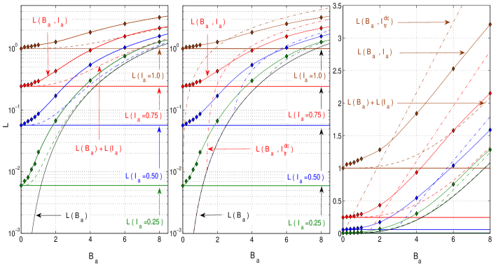
Figure 6.10: Hysteretic ac losses per cycle for synchronous AC magnetic flux density and oscillating transport current of amplitudes $(B_{\tt{a}},I_{\tt{a}})$ accordingly to the Figs. 6.4 & 6.9. Results of this work are shown as color solid lines with markers. Comparisons with results from conventional approaches are shown for, (i) Left pane: separate excitations $L(B_{\tt{a}})$ (black solid line) and $L(I_{\tt{a}})$ (straight color lines), as well as their linear superposition $L(B_{\tt{a}})+L(I_{\tt{a}})$ (color dashed lines); (ii) Central pane: an ac magnetic field together with a dc transport current of intensity $I_{\rm tr}^{\rm dc}=I_{\tt{a}}$ , $L(B_{\tt{a}},I_{\rm tr}^{dc})$; (ii) Right pane: the whole set of results is also plotted in linear scale. Units for losses are $(\mu_{0}/4\pi)\omega R^{2}J_{c}^{2}$.

First, let us recall that, according to Eq. (6.14) for isolated sources, the AC transport loss $L(I_{\tt{a}})$ may be calculated according to

$$L(i_{\tt{a}})\equiv\frac{\mu_{0}I_{c}^{2}}{\pi^{2}R^{2}}\left[i_{\tt{a}}\left(1-\frac{i_{\tt{a}}}{2}\right)+(1-i_{\tt{a}})\ln(1-i_{\tt{a}})\right]\,\leavevmode\nobreak\ \,\leavevmode\nobreak\ \,\forall\leavevmode\nobreak\ \,\leavevmode\nobreak\ \,0<i_{\tt{a}}\leq 1\,\,,$$ (6.29)

where the dimensionless parameter $i_{\tt{a}}=I_{\tt{a}}/I_{c}$ has been introduced.

On the other hand, the hysteretic loss produced by magnetization effects may be estimated from Eq. (6.18), in such manner that $L(B_{\tt{a}})$ is calculated from

$$L(b_{\tt{a}})\equiv\dfrac{8B_{p}^{2}}{3\mu_{0}}\left\{\begin{array}[]{ll}b_{\tt{a}}^{3}\leavevmode\nobreak\ \left(1-\dfrac{1}{2}b_{\tt{a}}\right)\nobreak\leavevmode\nobreak\leavevmode&,\leavevmode\nobreak\ \,\forall\leavevmode\nobreak\ \,\leavevmode\nobreak\ \,0<b_{\tt{a}}\leq 1\\ \\ b_{\tt{a}}-\dfrac{1}{2}\nobreak\leavevmode\nobreak\leavevmode&,\leavevmode\nobreak\ \,\forall\leavevmode\nobreak\ \,\leavevmode\nobreak\ \,b_{\tt{a}}\geq 1\,\leavevmode\nobreak\ \,\leavevmode\nobreak\ \,.\end{array}\right.$$ (6.33)

with the dimensionless parameter $b_{\tt{a}}=B_{\tt{a}}/B_{p}$. Recall that full penetration is given by $b_{\tt{a}}\geq 1$ (or $i_{\tt{a}}=1$).

The simplest approach for determining the AC losses of cylindrical superconducting wires subjected to synchronous AC excitations relies in the linear superposition of the separate contributions, $L(B_{\tt{a}})+L(I_{\tt{a}})$. Another possibility is to assume that the actual AC losses for synchronous excitations do not strongly differ of the hysteretic losses for superconducting samples carrying a constant transport current $I_{tr}^{dc}$ and a simultaneous oscillating magnetic field of amplitude $B_{\tt{a}}$ [57]. This idea was applied in the analytical approach by Zenkevitch et al. in Ref. [119]. In such a framework, the hysteretic loss for a period is approximated by:

$$L(B_{\tt{a}},I_{tr}^{dc})\equiv\dfrac{8B_{p}^{2}}{3\mu_{0}}\left\{\begin{array}[]{ll}b_{\tt{a}}^{3}\left(1-\dfrac{1}{2}b_{\tt{a}}\right)\nobreak\leavevmode\nobreak\leavevmode&,\leavevmode\nobreak\ \,\forall\leavevmode\nobreak\ \,\leavevmode\nobreak\ \,b_{\tt{a}}<i_{\tt{a}}^{{\dagger}}\\ \\ i_{\tt{a}}^{{\dagger}^{3}}\left(1-\dfrac{1}{2}i_{\tt{a}}^{{\dagger}}\right)+\left(1+i_{\tt{a}}^{2}\right)\left(b_{\tt{a}}-i_{\tt{a}}^{{\dagger}}\right)\nobreak\leavevmode\nobreak\leavevmode&,\leavevmode\nobreak\ \,\forall\leavevmode\nobreak\ \,\leavevmode\nobreak\ \,b_{\tt{a}}\geq i_{\tt{a}}^{{\dagger}}\,\leavevmode\nobreak\ ,\end{array}\right.$$ (6.37)

where we have introduced the dimensionless parameter $i_{\tt{a}}^{{\dagger}}\equiv 1-i_{\tt{a}}^{2/3}$ and the condition $b_{\tt{a}}\geq i_{\tt{a}}^{{\dagger}}$. Here, $I_{\tt{a}}\equiv I_{tr}^{dc}$. Thus, $b_{\tt{a}}\geq 1$ or $i_{\tt{a}}^{{\dagger}}\equiv 0$, both define a full penetrated sample.

Fig. 6.10 shows our numerical results for the variation of the actual AC losses of cylindrical SC wires in terms of the amplitude of the synchronous oscillating sources, $L(B_{\tt{a}},I_{\tt{a}})$ (solid-diamond lines), compared to the customary approaches $L(B_{\tt{a}})+L(I_{\tt{a}})$ (dashed lines at the left pane) and $L(B_{\tt{a}},I_{tr}^{dc})$ (dash-dotted lines at the central pane), for four different amplitudes of the AC/DC transport current $I_{\tt{a}}$, and a set of amplitudes of the AC density of magnetic flux $B_{\tt{a}}$. The whole set of results is also plotted in linear scale at the right pane of this figure.

Comparison reveals the important fact that a linear superposition of contributions due to either type of excitation may be only appropriate for high amplitudes of the magnetic field ($B_{\tt{a}}\geq B_{p}$) and low currents ($I_{\tt{a}}<I_{c}/4$), or the converse limit, very low magnetic fields ($B_{\tt{a}}\leq 1$) and extremely high currents $I_{\tt{a}}\lessapprox I_{c}$; a finding which adds to previous work dealing with a rectangular geometry [102] and sheds new light on the validity of approximate formulae at the same time. Actually, notice that the actual AC loss $L(B_{\tt{a}},I_{\tt{a}})$ is always higher than the instinctive approach $L(B_{\tt{a}})+L(I_{\tt{a}})$, whilst the deviation respect to $L(B_{\tt{a}},I_{tr}^{dc})$ strongly depends on the intensity of the electromagnetic excitations. Consequently, approximations such as $L\left(B_{\tt{a}}\right)+L\left(I_{\tt{a}}\right)$ and $L\left(B_{\tt{a}},I_{tr}^{dc}\right)$ can drastically under- or overestimate the true losses.

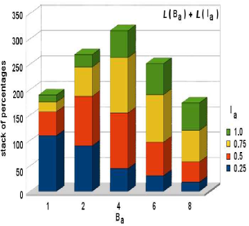
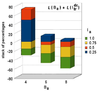
Figure 6.11: Percent change between the actual AC loss $L(B_{\tt{a}},I_{\tt{a}})$ numerically calculated and the intuitive approaches $L(B_{\tt{a}})+L(I_{\tt{a}})$ (left pane) and $L(B_{\tt{a}})+L(I_{tr}^{dc})$ (right pane).

For further understanding of the above behavior, Fig. 6.11 shows the percentage relation between the actual AC loss, $L(B_{\tt{a}},I_{\tt{a}})$, and the intuitive approaches, $L\left(B_{\tt{a}}\right)+L\left(I_{\tt{a}}\right)$ (left pane) and $L\left(B_{\tt{a}},I_{tr}^{dc}\right)$ (right pane), stacked according to the values of $I_{\tt{a}}$. On the one side, we note that for the approach $L\left(B_{\tt{a}}\right)+L\left(I_{\tt{a}}\right)$, and for small values of $I_{\tt{a}}$ (e.g. $I_{\tt{a}}=0.25$), the deviation is gradually reduced as one increases the amplitude of the magnetic field $B_{\tt{a}}$. However, as $I_{\tt{a}}$ increases deviations may either reduce (for low values of $B_{\tt{a}}$, e.g., $B_{\tt{a}}=1$) or increase (for high values of $B_{\tt{a}}$, e.g., $B_{\tt{a}}=8$). Moreover, for moderate fields (e.g., $2\leq B_{\tt{a}}\leq 6$) percentage deviations first grow as a function of $I_{a}$ until $I_{\tt{a}}=0.5I_{c}$, and then decrease as $I_{\tt{a}}$ approaches the current limit $I_{c}$. On the other side, the approach $L\left(B_{\tt{a}},I_{tr}^{dc}\right)$ is not even comparable with the actual AC losses $L(B_{\tt{a}},I_{\tt{a}})$ for the regime of low magnetic fields (particularly for $b_{\tt{a}}<i_{\tt{a}}^{{\dagger}}$), a range in which the approximation conceals the effect of $I_{a}$. However, for moderate and high magnetic fields, the percentage ratio between the actual AC loss and the AC loss predicted by the latter approach decrease as $I_{\tt{a}}$ increases even reaching negative values. Hence, $L\left(B_{\tt{a}},I_{tr}^{dc}\right)$ may either overestimate or underestimate the actual AC loss for wires subjected to synchronous oscillating sources. Remarkably, for high amplitudes of the oscillating magnetic flux density $B_{\tt{a}}$, we note that a synchronous oscillating transport current of amplitude $I_{\tt{a}}$ produces a lower amount of hysteretic losses per period, than those predicted when the superconducting sample is carrying a constant transport current $I_{tr}^{dc}$.

6.3.2  Asynchronous excitations

In many of the large-scale power applications for superconducting wires, such as windings of motors, transformers, generators and power three-phase transmission lines, the SC wire is subjected to diverse configurations of electromagnetic excitations, where the AC transport current flowing through and the magnetic field to which the wire is exposed could not fulfill the synchronous conditions referred above (same phase and frequency). Moreover, remarkable experimental differences between the AC loss measured for superconducting wires or tapes with synchronous and asynchronous oscillating transport current and perpendicular magnetic field have been already reported by several authors [99, 100, 101].

( A. ) General considerations on the “asynchronous” AC losses

Our analysis of the AC loss formulae for cylindrical superconducting wires subjected to simultaneous oscillating transport current $(I_{tr})$ and perpendicular magnetic flux density ($B_{0,y}$), has revealed that the total AC loss may be controlled by reducing the inductive magnetic flux density produced by the superposition between the external magnetic field and the contribution by the whole set of screening currents [recalling Eq. (6.12)]. This can be achieved just by a time shift respect to one of the AC electromagnetic sources (either $B$ or $I$) respect to the other, so that the occurrence of the peaks of excitation for each one of the electromagnetic sources is no longer synchronous with the other. Thus, some eccentric branches with opposite temporal derivatives appear between two consecutive peaks of the dominant excitation (i.e., the excitation with lower frequency this is the case), which may counterbalance the local variation of the magnetic flux density produced by the other one in the zone of maximum heat release.

Evidently, by competition between the magnetization currents and the so-called injected current lines, the magnitude of the local density of magnetic flux ($B_{i}$) may be reduced in half section of the superconducting cylinder shifting the relative phase between the electromagnetic excitations. Thus, as long as the electromagnetic excitations have the same oscillating period, reductions of the actual AC loss could be announced for shifts in the relative phase measured between the synchronous case and a temporal displacement of half period [i.e., $\Delta\phi=\pi$ if both sources accomplish the generic relation $f=f_{0}cos(\omega t+\phi)$], as it has been observed in Refs. [99, 100, 101]. Recall that, we have shown that the total AC loss decreases ensuring minimal variation of $\Delta B_{i}$ along the whole sample. In fact, if the relative phase shift equals half a period, it means that the occurrence of the excitation peaks for the electromagnetic sources are likewise synchronous but are pointing in opposite directions. Thus, as the total AC loss may be calculated by integration of the excitations peak to peak, for this case $\Delta B_{i}$ is maximum and therefore also the actual AC loss. On the other hand, the forecast of the minimal variation of the set of integrands in Eq. (6.12) and consequently the total AC loss, may be done by considering a temporal displacement of a quarter of period [i.e., $\phi=\pi/2$ for circular excitation functions], so that the local competition between the magnetic flux densities $\mid B_{0,i}\mid$ and $\mid B_{ind,i}\mid$ minimizes as $B_{0,y}(\Omega)=0$ when $\mid I_{tr}\mid=I_{a}$. Then, under this simplified scenario, and at least for cases where the local distribution of screening currents is current-like (very low magnetic field, $b_{a}\approx 0$, and high transport current, $i_{a}\approx 1$), or field-like (high magnetic field, $b_{a}\gtrsim 1$, and very low transport current, $i_{a}\approx 0$), the minimal AC loss is envisioned to appears for a relative phase difference of a quarter of period. Likewise, the maximal AC loss may be predicted when both sources are fully synchronous or when there is a relative phase shift of half period. Latter facts agree with the analytical approaches for the slab [124] and strip [125] geometries. Also, in further agreement with the experimental evidences of Refs. [99, 100, 101], within our statement we predict that as long as a phase shifting occurs, at least a minimal reduction of the AC loss should be observed.

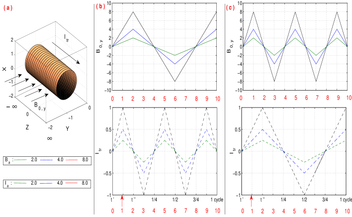
Figure 6.12: Sketch of some of the experimental processes analyzed along this chapter. Here, a cylindrical SC wire subjected to asynchronous oscillating excitations in the configuration shown in pane (a) are considered according to the temporal processes depicted in panes (b) and (c).

When the distribution of screening currents is “nothing-like”, i.e., it shows a strong deformation when compared to the obtained profiles for the isolated excitations, it is not obvious to deduce a general rule for the position of the maximum and minimum of the total AC loss, as the nonhomogeneous interplay between the injected current lines and the magnetization currents affects the total AC loss. In fact, the situation may be very much complicated for the actual applications of superconducting transformers and three-phase transmission lines [120, 121, 122, 123], by the fact that the self induced magnetic field and the external magnetic field may differ considerably in phase. Especially, one can foretell complicated behaviors when effects of phase transposition and, frequency shifts appear. Here, we will show how the effects of double frequency which may be occasionally found in the power supply networks, can drastically alter the efficiency of the superconducting machines.

Fig. 6.12, shows the configuration analyzed below. Notice that, in what follows, we consider the effect of introducing one of the excitations with an oscillating frequency twice as big as the other. Thus, calculation of the AC loss, i.e., integration of the local density of power dissipation $\textbf{E}\cdot\textbf{J}$ is made along the smaller frequency excitation. In detail, we have considered the following cases:

1. The injected transport current is the source within the double frequency regime [see Fig. 6.12 (b)], and

2. The temporal dynamics of the magnetic flux density associated to the external source of magnetic field shows a double frequency behavior [see Fig. 6.12 (c)].

Most remarkable features for the flux dynamics, magnetic response, and AC losses for the above mentioned configurations are detailed below.

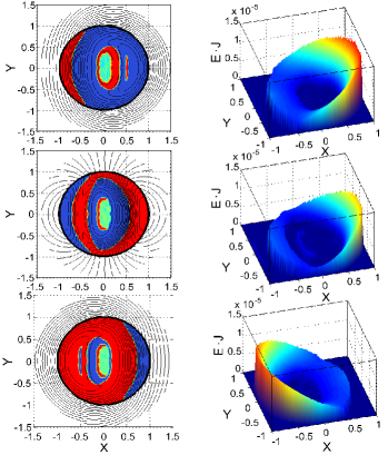
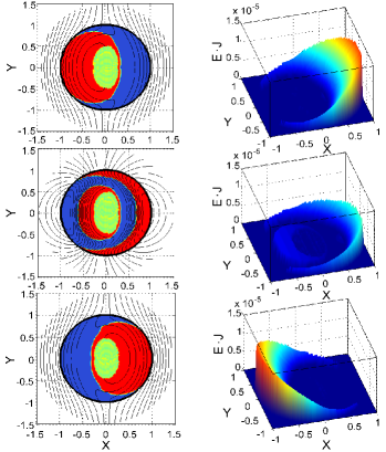
Figure 6.13: Evolution of the magnetic flux lines and their corresponding profiles of current with asynchronous oscillating sources $B_{0,y}$ and $I_{tr}$ of amplitudes $B_{\tt{a}}=4$ and $I_{\tt{a}}=0.5$ (left side into each pane), accordingly to the temporal processes displayed into Fig. 6.12(b) “left pane herein” and Fig. 6.12(c) “right pane herein”. Also the corresponding profiles for the local density of power dissipation E$\cdotp$J are shown (right side into each pane). In particular, in this figure we show the set of results for the last branch of the dominant excitation according to the time-steps marked with the labels (6), (8), and (10) in Fig. 6.12. More details to follow up the electromagnetic quantities along the cyclic process are found in the section of supplementary material, pages II-II.

( B. ) Flux dynamics

Before discussing the results obtained for the total AC loss in the set of experiments displayed in Fig 6.12, some outstanding facts related to the rich phenomenology found for the local dynamics of the electromagnetic quantities are worth of mention. For example, when the applied magnetic field and the transport current are synchronous, and their associated amplitudes $(B_{\tt{a}},I_{\tt{a}})$ are weak enough such that a flux-free core remains along the AC cycles (i.e., as long as $i_{\tt{a}}^{*}\neq 1$ and $b_{\tt{a}}^{*}<1$), it is more or less simple to identify the active zones in the AC cycles via the previous knowledge of the virgin branch (see Figs. 6.5 & 6.6, pags. 6.5-6.6), and therefore, explaining and obtaining the AC loss may be achieved if the distribution of screening currents is well known for the first half of the AC period. However, when the temporal dynamics of the isolated excitations shows an asynchronous response, this is not longer valid. The reason is, that the hysteretic losses produced along the virgin branch are not monotonic concerning the temporal evolution of both electromagnetic excitations, such that the accruing hysteretic losses for the lower limit in the first integral of Eq. (6.27) are different for the first and second half of the cyclic period. In other words, the distribution of screening currents in the first peak of the excitation with smaller frequency or below so called dominant excitation [time step 2 in Fig. 6.12] may drastically differ from those conceived in the second and third peaks [time steps 6 and 10]. Hence, the distribution of screening currents for the first half period of the AC cycle cannot be fetched through their distribution in the virgin branch. Therefore, we want to call reader’s attention to the fact that for making use of Eq. (6.27) for the calculation of AC losses, the steady regimes for the limits of the time-integral have to be defined for the excitation peaks defining the second half period of the dominant excitation. Thus, a proper description of the profiles of current density in an asynchronous AC regime must be done at least for this temporal branch (see Fig. 6.13).

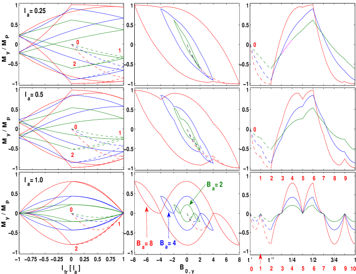
Figure 6.14: The dimensionless magnetic moment $M_{y}/M_{p}$ for the AC asynchronous excitations displayed in Fig. 6.12(b) where the applied magnetic field have the role of dominant excitation. Curves are shown as function of the injected transport current $I_{tr}$ in units of their amplitude $I_{\tt{a}}$ (left column), the applied magnetic field $B_{0,y}$ (central column), or either by its temporal evolution (right column). Same color scheme to point out the amplitude of the AC magnetic field ($B_{\tt{a}}$) has been used in all subplots.

Analyzing the distribution of current density profiles in Fig. 6.13 and their corresponding profiles for the local density of power dissipation $\textbf{E}\cdot\textbf{J}$, we found at least two interesting facts which are worth of mention. On one side, whether it is the magnetic field or the transport current, the excitation which leads the role of dominant, multiple domains or active zones connected between them may appear, which makes it impossible to find out a feasible analytical solution for the flux front boundary in the infinite spectra of combinations between the amplitudes $B_{\tt{a}}$ and $I_{\tt{a}}$, specially if the pattern of current density is far away of the approaches for profiles of the kind current-like or field-like. On the other side, a most striking fact revealed in Fig. 6.13 is that contrary to the behavior displayed for the local profiles of density of power dissipation $\textbf{E}\cdot\textbf{J}$, when both electromagnetic excitations are synchronous (see e.g. Fig. 6.7, pag. 6.7), in asynchronous cases the zone of heat release is no longer localized in one side of the superconducting sample. Thus, the idea of focusing heat release in some part of the superconductor requires a special attention in the synchronization of sources.

( C. ) Magnetic response

Another interesting feature which derives from the study of asynchronous excitations is the actual possibility of finding “exotic” magnetization loops as a function of the AC sources (see Figs. 6.14 & 6.15), where the straightforward competition between the magnetization currents (by consumption) and the injected current lines, may be visualized in terms of a non local macroscopic measurement.

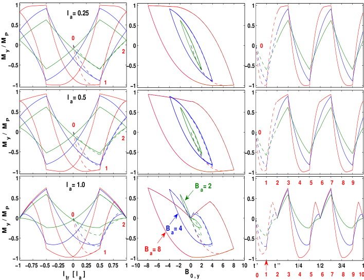
Figure 6.15: The dimensionless magnetic moment $M_{y}/M_{p}$ for the AC asynchronous excitations displayed in Fig. 6.12(c) where the transport current has the role of dominant excitation. Curves are shown as function of the injected transport current $I_{tr}$ in units of their amplitude $I_{\tt{a}}$ (left column), the applied magnetic field $B_{0,y}$ (central column), or either by its temporal evolution (right column). Same color scheme to point out the amplitude of the AC magnetic field ($B_{\tt{a}}$) has been used in all subplots.

In Fig. 6.14, the component of magnetic moment $M_{y}$ is displayed for the AC process in Fig. 6.12(b), where the AC magnetic field dominates the cyclic period of excitation. The whole set of results for $M_{y}$ have been renormalized according to the maximal expected value for the magnetic moment when only applied magnetic field is considered ($M_{p}=2/3$). Thus, curves are shown as function of the isolated electromagnetic excitations, $I_{tr}$ (in units of their associated AC amplitude $I_{\tt{a}}$) at the left column, $B_{0,y}$ at the central column, as well as by the time defining the first steady-period (right column). Notice that, the virgin branch which does not play any role for the integration of the AC losses per cyclic periods is shown through dashed lines. Furthermore, results have been organized accordingly to the associated amplitudes for the applied density of magnetic flux $B_{\tt{a}}$, such that $B_{\tt{a}}=2$ corresponds to the green curves, $B_{\tt{a}}=4$ to the blue curves, and $B_{\tt{a}}=8$ to the red curves. Likewise, the set of curves shown for each row can be straightforwardly associated to a single value for the amplitude of the AC transport current, $I_{\tt{a}}=0.25$ (first row), $I_{\tt{a}}=0.5$ (second row), and $I_{\tt{a}}=1$ (third row). Analogously, the corresponding set of curves obtained for the component of magnetic moment $M_{y}$ in those cases where the AC transport current dominates the cyclic period of excitation, are shown in the same fashion above described in Fig. 6.15.

Outstandingly, whether $B_{0,y}$ (Fig. 6.14) or $I_{tr}$ (Fig. 6.15) is the dominant excitation, and for low values of $I_{\tt{a}}$, the magnetization loops as function the magnetic flux density $M_{y}(B_{0,y})$ show a Bean-like behavior. As the value of $I_{\tt{a}}$ increases, notorious deformations of the Bean-like structures for the magnetic moment appear. Nevertheless, the behavior is radically different comparing the double frequency effects provided by one or another excitation, as it is explained below.

( i. ) Transport current with double frequency

On the one hand, when it is the AC transport current, $I_{tr}$, that shows a double frequency, the magnetization curves $M_{y}(B_{0,y})$ display a symmetric behavior in the regions (left-right) of the periods $[B_{\tt{a}}\Rightarrow-B_{\tt{a}}]$ and $[-B_{\tt{a}}\Rightarrow B_{\tt{a}}]$ (see Fig. 6.14). On the contrary, for $M_{y}(I_{tr})$, one can notice the existence of a symmetrization of the curves of magnetic moment regarding their positive and negative values (up/down). Evidently, the steady-states where the maximum consumption of the magnetization currents occurs, always arise when the asynchronous AC excitation $[B_{0,y},I_{tr}]$ reaches the values for the current’s peaks [see Fig. 6.12(b)], i.e., for the time-steps (3) $[B_{\tt{a}}/2,-I_{\tt{a}}]$, (5) $[-B_{\tt{a}}/2,I_{\tt{a}}]$, (7) $[-B_{\tt{a}}/2,-I_{\tt{a}}]$, and (9) $[B_{\tt{a}}/2,I_{\tt{a}}]$. Then, by increasing (decreasing) the value of $I_{\tt{a}}$, a progressive decreasing (increasing) of the magnetic moment at these points ends up in the simultaneous collapsing of the magnetization curves $(M_{y}\equiv 0)$ for the half periods of the dominant excitation $B_{0,y}$, as long as $I_{\tt{a}}=\pm I_{c}$. Latter fact is followed by the symmetrization of the loops, either as functions of $B_{0,y}$ and $I_{tr}$, into characteristic lenticular shapes bounded by two non-connected magnetization curves, both defined by the elapsed periods in which the time derivative of $I_{tr}(t)$ is positive, i.e., for the temporal branches $(3\Rightarrow 5)$ and $(7\Rightarrow 9)$. Then, the connecting curves for the abovementioned magnetization branches shows characteristic lashing shapes when the time derivative of $I_{tr}(t)$ is negative. Remarkably, as a consequence of this process, the output signal $M_{y}(t)$ does not show the low-pass filtering effects conceived for synchronous excitations. In fact, given our study, we prove that the low-pass filtering effect for superconducting wires, may only be envisaged when the temporal evolution of the injected AC transport current and the perpendicular magnetic field is fully synchronous (in phase and frequency).

( ii. ) Applied magnetic field with double frequency

On the other hand, when it is the AC density of magnetic flux, $B_{0,y}$, the electromagnetic source disclosing the double frequency effect [Fig. 6.12 (c)], the calculated curves of magnetization $M_{y}(B_{0,y})$, are outstandingly different. Thus, there are no symmetry conditions which may be observed in this representation (2nd column in Fig. 6.15). However, for the set of magnetization curves as a function of the transport current, $M_{y}(I_{tr})$, we have noticed a well-defined symmetrization of the magnetization loops regarding to the positive and negative values of $I_{tr}(t)$ (left/right). Notwithstanding, in terms of the magnetization curves $M_{y}(B_{y})$, there is also a further fact to be mentioned. Strikingly, by using this representation it is possible to note that the steady-states where the consumption of the magnetization currents becomes evident, are mainly present along the period in which the time derivative of $B_{0,y}(t)$ is negative, whilst the AC transport current evolves through the current’s peaks, i.e., for the temporal branches defined by the time-steps (1) $[B_{\tt{a}},I_{\tt{a}}/2]$ to (3) $[-B_{\tt{a}},I_{\tt{a}}/2]$, and (5) $[B_{\tt{a}},-I_{\tt{a}}/2]$ to (7) $[-B_{\tt{a}},-I_{\tt{a}}/2]$. Moreover, the magnetic response of the superconductor is not monotonic along these branches. For example, from the time step (5) until the time step (6) $[0,-I_{\tt{a}}]$, the electromagnetic excitations, $B_{0,y}$ and $I_{tr}$, have the same tendency (both decreasing). However, if $I_{\tt{a}}$ tends to the limiting value $I_{c}$, $M_{y}$ may increase and decrease within the same period. Then, from the time step (6) to the time step (7) both evolve in opposite directions, but however the magnetic moment always increases along this period. On the other hand, for the following analogous branch in the AC period of magnetic field, say the time-steps (9) to (11), the magnetic moment curve is the same, but the competition between the electromagnetic sources $B_{0,y}$ and $I_{tr}$ is opposite to the aforementioned evolution. Thus, depending on the intensities of the electromagnetic sources, both reduction or enhancement of the hysteretic AC losses may envisaged when there is a difference between the oscillating excitation frequencies. Recall that, in contrast, by assuming only a relative difference in phase, only reductions of the actual AC loss may be foretell.

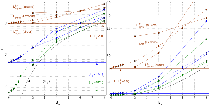
Figure 6.16: Hysteretic AC losses per cycle for asynchronous sources accordingly to the excitations shown in Fig. 6.12(b) “Herein, $L_{asynch}^{(b)}$ : square-solid-lines”, and Fig. 6.12(c) “Herein, $L_{asynch}^{(c)}$ : circle-solid-lines”. The results are compared with the curve of losses for synchronous sources, $L_{synch}\equiv L(B_{\tt{a}},I_{\tt{a}})$ predicted above (Fig. 6.10), and the curves for isolated excitations $L(B_{\tt{a}})$ and $L(I_{\tt{a}})$. The whole set of results is also plotted in linear scale. Units for losses are $(\mu_{0}/4\pi)\omega R^{2}J_{c}^{2}$.

( D. ) AC Losses in asynchronous systems

In Fig. 6.16, the hysteretic AC loss calculated for the experimental configurations conceived in Fig. 6.12 [panes (b) and (c)] are shown. To be specific, $L_{asynch}^{(b)}$ and $L_{asynch}^{(c)}$, are shown in terms of the amplitude of the applied density of magnetic flux $B_{\tt{a}}$, whilst the different values for $I_{\tt{a}}$ are pointed in terms of the sequence of colors for the DC loss curves depicted in Fig. 6.10 (pag. 6.10). Likewise, results are compared with the corresponding curves for the actual AC loss when the synchronous electromagnetic excitations were considered, i.e., $L_{synch}\equiv L(B_{\tt{a}},I_{\tt{a}})$. Outstandingly, for both cases, remarkable variations of the AC loss occur. Thus, with the aim of providing a clearest understanding of the range of variations in the AC loss curve for the configurations abovementioned, and further help the readers in the visualization of the numerical data, in Fig. 6.17 we show the percentage relation between the calculated losses for synchronous excitations, $L_{synch}$, and the calculated losses for the asynchronous cases, $L_{asynch}^{(b)}$ and $L_{asynch}^{(c)}$.

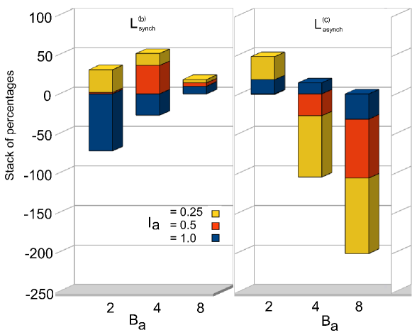
Figure 6.17: Percent change between the AC loss for synchronous excitations, $L_{synch}$, and the losses $L_{asynch}^{(b)}$ (at the left-side) and $L_{asynch}^{(c)}$ (at the right-side), for combinations of three different amplitudes $B_{\tt{a}}$ and $I_{\tt{a}}$.

Notice that, on the one hand, when the applied magnetic field provides the dominant oscillating period (the impressed AC transport current shows a relative double frequency, Fig. 6.12(b)), the resulting comparison between the calculated losses $L_{asynch}^{(b)}$ and $L_{synch}$ for high values of $B_{\tt{a}}$ [Fig. 6.17], shows a small but sizable increase of the hysteretic loss as a consequence of the double frequency effect ($\sim 4-10\%$ for $B_{\tt{a}}\equiv B_{p}=8$). Then, assuming that $I_{\tt{a}}\equiv I_{c}=1$, we have found that the AC loss reduces as $B_{\tt{a}}$ decreases. However, an outstanding fact is that for the lowest values of $B_{\tt{a}}$ and $I_{\tt{a}}$, a notorious increase of the actual AC losses appears. For example, for $B_{\tt{a}}=B_{p}/2=4$ and $I_{\tt{a}}=I_{c}/2=0.5$, deviation is about $36\%$. Likewise, for $B_{\tt{a}}=B_{p}/4=2$ and $I_{\tt{a}}=I_{c}/4=0.25$, deviation is about $29\%$

On the other hand, when the electromagnetic source with the double frequency is the applied magnetic field [Fig. 6.12(c)], the resulting AC loss ($L_{asynch}^{(c)}$) for high values of $B_{\tt{a}}$ shows a significant reduction as compared to the predicted losses for synchronous configurations ($\sim 95\%$ for $B_{\tt{a}}\equiv B_{p}=8$ and $I_{\tt{a}}\equiv I_{c}/4=0.25$). However, by reducing $B_{\tt{a}}$ a notorious increase of the AC loss may be revealed depending on the value of $I_{\tt{a}}$. In fact, we call readers’ attention about the relative increase of the AC losses as compared to those of the synchronous cases: $\sim 14\%$ for ($B_{\tt{a}}=4$ , $I_{\tt{a}}=1$), and $\sim 18\%$ for ($B_{\tt{a}}=2$ , $I_{\tt{a}}=1$). Moreover, for those cases with the lower values of $B_{\tt{a}}$, i.e., $B_{\tt{a}}=2$, increases of the AC loss are also found for $I_{\tt{a}}=0.25$ ($\sim 29\%$), whilst for the intermediate case [$B_{\tt{a}}=2$,$I_{\tt{a}}=0.5$], it shows a reduction of the AC loss of less than 1%. The remarkable point here, is that for asynchronous excitations of $B_{0}$ and $I_{tr}$, reductions of the AC losses can be only asserted if both sources evolve with the same frequency, i.e.: if one is restricted to shifts in phase.

Conclusions II

In this part, we have shown that our general critical state theory for the magnetic response of type-II superconductors in the framework of optimal control variational theory and computational methods for large scale applications may be applied in an extensive number of configurations.

In order to summarize the main physical features extracted from our numerical experiments, the conclusions are presented according to the previous sequence of chapters as follows:

Chapter 4

General critical state problems have been solved for a wide number of examples within the infinite slab geometry. All of them share a three dimensional configuration for the magnetic field, i.e., ${\bf H}=(H_{x},H_{y},H_{z})$, under various magnetic processes, and different models for the critical current restriction or material law. Thus, we have considered several physical scenarios classified by the ansatz for the flux depinning and cutting processes (basically affecting the critical current thresholds $J_{c\perp}$ and $J_{c\parallel}$), their relative importance (given by $\chi\equiv J_{c\parallel}/J_{c\perp}$), and a coupling index $n$ which controls the smoothness of the material law. In summary, the following scenarios have been analyzed:

1. Isotropic solutions, in which the limiting case with $\chi^{2}=1$ and $n=1$ produces states under the 1D constraint $J=J_{c}$.

2. T-state solutions, in which the approximation $\leavevmode\nobreak\ \chi\gg 1$ produces the result $J_{\perp}=J_{c\perp}$, and $J_{\parallel}$ may be arbitrarily high. Our predictions show an excellent agreement with previous analytical results in the literature, and extend the theory to the full range of applied magnetic fields.

3. CT-state solutions in which $\chi\geq 1$ for several cases within the rectangular region given by the threshold conditions $J_{\perp}\leq J_{c\perp}$ and $J_{\parallel}\leq J_{c\parallel}$ are analyzed. Outstandingly, the appearance of the flux cutting limitation takes place as a sudden corner in the magnetic moment curves in many cases. The corner establishes a criterion for the range of application of T-state models.

4. SDCST solutions, in which the possible coupling between the flux depinning and cutting limitations has been studied through the solution of smoothed DCSM cases. In particular, we consider the effect of rounding the corners of the rectangular region $J_{\perp}\leq J_{c\perp}$ and $J_{\parallel}\leq J_{c\parallel}$, by the superelliptic region criterion $(J_{\parallel}/J_{c\parallel})^{2n}+(J_{\perp}/J_{c\perp})^{2n}\leq 1$ with $1\leq n<\infty$. It is shown that, under specific conditions (paramagnetic initial state and low perpendicular fields), important differences in the predictions of the magnetic moment behavior are to be expected. The differences in ${\bf M}$ have been related to the behavior of the critical current vector ${\bf J}_{c}$ around the corner of the rectangular region.

Remarkably, the whole set of physical features linked to the different material laws may be depicted in terms of the magnetization curves for the aforementioned experimental configurations [see Fig. 4.2, pag. 4.2]. The main findings are synthesized in figure II-1.

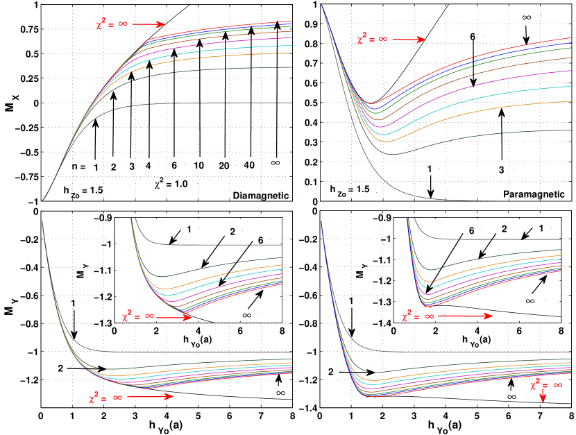
Figure II-1: The magnetic moment components of the slab $M_{x}$ (top) and $M_{y}$ (bottom) per unit area as a function of the applied magnetic field $h_{y_{0}}$ for the experimental configurations depicted in Fig. 4.2. By comparison, results for several models in the diamagnetic (left panes) and paramagnetic (right panes) configurations are shown. In terms of our SDCST we display the magnetization curves for: the infinite bandwidth model or so called model of T-states ($\chi^{2}\rightarrow\infty$, $J_{c\perp}\neq 0$), the conventional DCSM ($\chi^{2}=1$, $n\rightarrow\infty$), several material laws defined by the superelliptical regions $\chi^{2}=1$ and $n=2$, 3, 4, 5, 6 and 10, and finally the isotropic model or superelliptical region with $\chi^{2}=1$ and n=1.

Firstly, we have noticed a pronounced peak effect in both components of the magnetic moment. We emphasize that whatever region is considered [excepting the limiting cases “$\chi^{2}=1$, $n=1$” (isotropic model), and “$\chi^{2}\to\infty$” (T- or infinite bandwidth- model)], the peak effect in the paramagnetic case is predicted for both components of the magnetization. Thus, we argue that the peak effect cannot be interpreted as a direct evidence of an elliptical material law. Instead of this, it is a universal signal of the anisotropy effects involved in a general description of the material law. The evolution of the peak effect as a function of $\chi^{2}$ has been shown in Fig. 4.15 (pag. 4.15). There, we note that an increase of the bandwidth $\chi^{2}$ produces a stretched magnetic peak. Consequently, paramagnetic effects are visible over a wider range as the cutting threshold value $J_{c\parallel}$ increases. We also emphasize that the overall effect of increasing the value $\chi^{2}=(J_{c\parallel}/J_{c\perp})^{2}$ is that the components of ${\bf M}$ get closer to the master curves defined by $\chi\to\infty$.

Secondly, some additional and distinctive signals for the different models have been also observed. On the one hand, for the isotropic model, the collapse of the magnetization is achieved while $J_{\parallel}$ is monotonically reduced [Figs. 4.3 – 4.5, pags. 4.3 – 4.5]. When the material law is the infinite bandwidth model ($\chi^{2}=\infty$, or so called T-state model) the magnetization collapse does not occur, and there is no restriction on the longitudinal component of the current that increases arbitrarily towards the center of the sample [Figs. 4.6 – 4.10, pags. 4.6 – 4.10]. This corresponds to the absence of flux cutting, i.e.: $J_{\parallel}$ does not saturate by reaching a threshold value $J_{c\parallel}$. For rectangular or smooth rectangular regions [Figs. 4.11 – 4.15, pags. 4.11 – 4.15], together with the absence of collapse, one also observes that $J_{\parallel}$ basically saturates to a value that depends on the smoothing parameter $n$ (exactly to $J_{c\parallel}$ for the very rectangular case $n\to\infty$). Remarkably, when a rectangular section is assumed, the sample globally reaches the CT state (corner of the rectangle). As a consequence of the sharp limitation for $J_{\parallel}$, a well-defined corner in the magnetic moment components $M_{x}$ and $M_{y}$ appears, both for the diamagnetic and paramagnetic cases (see e.g., Fig. II-1). This clear trace of the DCSM establishes the departure from the master curves defined by the T-state, and has been assigned to the instant at which the sample reaches the CT state.

Let us call the readers’ attention about a noticeable gap in Fig. II-1, separating the isotropic model ($\chi^{2}=1,\leavevmode\nobreak\ n=1$) and the square model ($\chi^{2}=1,\leavevmode\nobreak\ n\to\infty$). In fact, if one compares Fig. II-1 and Fig. 4.15 (pag. 4.15) one can realize that smooth models for a given ratio $\chi\equiv J_{c\parallel}/J_{c\perp}$ will fill the gap between the master limiting curves defined by the rectangular ($\chi,n\to\infty$) and elliptic ($\chi,n=1$) models, and their corresponding curves for different values of $\chi$ will intersect in a complicated fashion. In this sense, we argue that the magnetization curves by themselves do not provide unambiguous information on the material law which defines the critical state dynamics in type II superconductors. Moreover, notice that in the regime of low fields $H_{z}\sim h_{y}(a)$ the material law is indistinguishable and the magnetic moment may be reproduced even by the isotropic model. However, we have noticed that, although the dynamics of the profiles $H_{x}$, $J_{y}$, and $J_{x}$ is almost indistinguishable between the smooth and rectangular models a clear distinction arises by analyzing $J_{c\parallel}$. On the one hand, when the rectangular model is assumed $J_{\parallel}$ reaches the threshold value $J_{c\parallel}$, and the entire specimen verifies a CT-state as the applied magnetic field increases. On the other hand, when the rectangular region is smoothed by the index $n$, the parallel component of the current density eventually decreases to a value that depends on the values of $n$ and $\chi$. Thus, further research along this line is suggested [46], i.e.: the design of some experimental routine that defines a well posed inverse problem for the determination of $\Delta_{\textbf{r}}$.

Finally, in Appendix-I the critical angle (between vortices) criterion that establishes the limitation on $J_{\parallel}$ has been modified for 3D problems. It is shown that, in general, the concept may involve both $J_{\parallel}$ and $J_{\perp}$ as one can see in Eqs. (4.12) & (4.15). Nevertheless, the influence of the local magnetic anisotropy and the underlying effects at the flux cutting mechanism are much less noticeable, especially for the diamagnetic case, in which the full range of physically meaning values of $\kappa_{c}$ produce a negligible variation.

Chapter 5

Despite of extensive experimental and theoretical studies about the electrodynamic response of type-II superconductors in longitudinal geometries, much uncertainties remain about the interaction between flux depinning and cutting mechanisms, and their influence in such striking observations as the appearance of negative transport current flow, the enhancement of the critical transport current density, and the observation of peak effects on the magnetization curves. In this chapter, and based on the application of our SDCST, we have reproduced theoretically the existence of negative flow domains, local and global paramagnetic structures, emergence of peak-like structures in the longitudinal magnetic moment, as well as the compression of the transport current density for a wide number of experimental conditions.

Here, the longitudinal transport problem in superconducting slab geometry has been studied as follows: on the one hand, we have considered a superconducting slab lying at the $xy$ plane and subjected to a transport current density along the $y$ direction as it is shown in the left pane of Fig. 5.3 (pag. 5.3). The slab is assumed to be penetrated by a uniform vortex array along the $z$ direction, so that the local current density along the thickness of the sample is entirely governed by the depinning component ($J_{\perp}$) perpendicular to the local magnetic field. Subsequently, a magnetic field source parallel to the transport current direction is switched on. Then, the experimental conditions have been changed through the value of the external magnetic field $H_{y0}$.

The dynamical behavior of the transport current density is shown to rely on the interaction between the cutting and depinning mechanisms. Moreover, the intensity of the inherent effects has been shown to depend on the perpendicular component $H_{z0}$, being more prominent as this quantity is reduced. In fact, for restricted situations (infinite slab geometry and only fields parallel to the surface, $H_{z0}=0$), we have shown that the prediction of the counterintuitive effect of negative current flow in type-II superconductors may be even predicted within a simplified analytical model (section 5.1.1). Then, the three-dimensional effects are straightforwardly incorporated by numerical methods when the third component of the local magnetic field ($H_{z}$) is considered.

By means of our SDCST that allows to modulate the influence of the different physical events, by using a superelliptical material law that depends on two parameters ($\chi\equiv J_{c\|}/J_{c\perp}$ and $n$) accounting respectively for the intrinsic material anisotropy and for the smoothness of the $J_{\parallel}(J_{\perp})$ law, we have quantitatively investigated the influence of the flux cutting mechanism and shown that the peak structures observed in the magnetization curves and the patterns of the transport current along the central section of a superconducting sample are both directly associated with the local structure of the vortex lattice. Such dependence may become more pronounced as the extrinsic pinning of the material is reduced, in favor of the flux cutting interactions. The same conclusion was pointed out from the experimental measurements of Blamire et.al. (Ref. [26, 27]) for high critical temperature and conventional superconductors. It has been done by comparing the T-state model ($\chi\to\infty$), and the smooth double critical state conditions CT$\chi$ with $\chi=1$, 2, 3 and 4, all of them with the smoothing index $n=4$ and $J_{c\perp}=1$. Going into detail, when the cutting threshold is high ($J_{c\|}\gg J_{c\perp}$ or $\chi\gg 1$) the emergence of negative current patterns is ensured because unbounded parallel current density allows unconstrained rotations for the flux lines as the longitudinal magnetic field increases. Thus, under a range of conditions, the peak effects in the magnetic moment and a modulation of the negative surface currents have been predicted.

Only for completeness, it is to be mentioned that from our theoretical framework we have obtained that the isotropic model (circular region: $\chi=1$, $n=1$) does neither predict the appearance of negative current patterns nor the peak effects in the magnetic moment curves. However, as long as a clear distinction between the depinning and the cutting components of $\bf J$ is allowed (by letting $n>1$), several remarkable facts can be explained.

In order to understand the different consequences and physical phenomena derived from the SDCST for the longitudinal transport problem, our numerical results may be summarized as follows:

1. For the magnetic process under consideration [Fig. 5.3, pag. 5.3], and concentrating on the local properties within the sample [see e.g., Fig. 5.4, pag. 5.4], a clear independence of the field and current density profiles relative to the anisotropy level of the material law has been obtained for the partial penetration regime, in which the flux free core progressively shrinks to zero [top pane of Figs. 5.7 – 5.10, pags. 5.7 – 5.10].

2. Negative values for the transport current density $j_{y}$ are neither obtained for the T or CT$\chi$ states when $h_{z0}$ is high ($h_{z0}\gtrsim 50$) until extreme values of the longitudinal field ($h_{y0}\gtrsim 500$) are reached [see e.g., $j_{y}(a)$ profiles in Figs. 5.5 (pag. 5.5), 5.11 (pag. 5.11) & 5.12 (pag. 5.12)]. On the contrary, one can early find negative current flow for both cases when $h_{z0}\leq 2$. Notice by Eq. (5.1), pag. 5.1, that the reduction of the perpendicular component of the magnetic field may be understood as an enhancement of the cutting current component. Thus, the negative values of ${j}_{y}(z)$ are obtained for smaller and smaller $h_{y0}$ as $h_{z0}$ also decreases. In fact, negative values can happen even for the partial penetration regime ($h_{y0}\lesssim 0.845$) when $h_{z0}$ tends to $0$, in accordance with the analytical model presented before (Section 5.1.1).

3. If $j_{\parallel}$ is unbounded (T states) the ${j}_{y}(z)$ structure becomes rather inhomogeneous as $h_{y0}$ increases and takes the form of a highly positive layer in the center shielded by a prominent negative region, i.e., the transport current is essentially compressed toward the center of the sample by the effect of the shielding currents. Also, it is worth of mention that, when simulating experiments in which the transport current is applied subsequent to the field, the SDCST does not predict negative flow values at all. On the contrary, in such cases, what one gets is a compression of the original field penetration profile, until the increasing transport current leads to dissipation.

4. When $j_{\parallel}$ is bounded (CT states) one observes a negative layer at the surface that eventually disappears when $h_{y0}$ increases more and more [e.g., $h_{y0}>100$ for CT1 case - see bottom pane of Fig. 5.11 (pag. 5.11)]. Thus, as a general rule, the smaller the value of $h_{z0}$, the sooner the negative transport current is found. In the CT cases, this also increases the range of longitudinal field for which negative values are observed.

5. The peaked structure of $j_{y}(z)$ for the T-states at $h_{z0}=0.5$ is accompanied by a similar behavior in $j_{x}(z)$ that relates to a subtle magnetic field reentry phenomenon in $h_{y}(z)$ [see curves labeled $h_{y0}=10$ in the bottom pane of Fig. 5.4 (pag. 5.4)]. For the corresponding CT$\chi$ cases, the occurrence of this phenomena is linked to the choice of widthbands larger than $\chi=1$ [by comparison, see profiles for the labeled first stage at the bottom of Fig. 5.8 (pag. 5.8)].

6. Unlimited growth of the global magnetic moment component $M_{x}$ as a function of the longitudinal magnetic field $h_{y0}$ occurs for the T-states in which $j_{\parallel}$ is unbounded. From the local point of view, this relates to an unlimited growth (compression) of the current density at the center of the slab [$j_{y}(0)$]. Remarkably, the appearance of a peak structure in $M_{x}(h_{y0})$ correlates with the maximum value of the transport current density at the center of the slab for the bounded CT states. For example, for the CT1 case (square with $\chi=1$ and a smoothed corner by $n=4$) the obtained maximum value $j_{y}^{max}(0)=1.2968$ corresponds to the optimal orientation of the region $\Delta_{\textbf{r}}$ in which the biggest distance within the superelliptic hypothesis is reached. Such situation is sketched in Fig. 4.1 (pag. 4.1) and one may check the numeric result from the expression

   $${\rm Max}\{j_{c\parallel}(\Delta_{\textbf{r}})\}=j_{y}^{max}=\left(1+\chi^{2n/(n-1)}\right)^{(n-1)/2n}\,.$$

   Notice that, as a limiting case, it produces the expected value $2^{1/2}$ for the diagonal of a perfect square [i.e., $n\to\infty$ in Eq. (2.19), pag. 2.19].

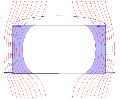
Figure II-2: Penetration of a magnetic field parallel to the axis of a finite superconducting cylinder (only one radial cut for the longitudinal section is shown for symmetry reasons). The component of the magnetic field perpendicular to the lateral surface is visualized by a set of arrows with normalized lengths. The central dashed line represents the symmetry axis.

Additional physical considerations can be done so as to cover the full experimental scenario for the longitudinal transport problems. In particular, although our analysis has been performed within the infinite slab geometry, one can straightforwardly argue about the extrapolation to real experiments by means the inclusion of the third component of the magnetic field, $H_{z0}$, which qualitatively may be related to the importance of the finite size effects in real superconducting samples. Notice that our numerical calculations, imply that negative currents should be more prominent in those regions of the sample where the component of ${\bf H}$ perpendicular to the current density layers is less important. Thus, considering that a real sample in a longitudinal configuration will be typically a rod with field and transport current along the axis, the above idea is straightforwardly shown by plotting the penetration of an axial field in a finite cylinder (see Fig. II-2). Then, the aforementioned effect will occur at the central region of the sample, where end effects are minimal.

Just for visual purposes, Fig. II-2 shows the distortion of the magnetic field, shielded by the induced supercurrents in a finite superconducting cylinder, where the horizontal component of the magnetic field along the lateral surface layer has been outlined. It is apparent that the normal component of ${\bf H}$ will be enhanced close to the bases and tend to zero at the central region. Then, inhomogeneous surface current densities with negative flow at the mid part should be expected in agreement with the experimental evidences reported in Refs. [7, 35, 36, 22, 37, 38, 39, 21, 40, 41, 42, 43, 44, 45].

Chapter 6

In this chapter, we have presented a thorough study of the local and global electromagnetic response of a straight, infinite, cylindrical type-II superconducting wire subject to diverse AC-configurations of transverse magnetic flux density $B_{0}(t)$ and/or longitudinal transport current flow $I_{tr}(t)$. We have assumed that the superconductor follows the celebrated critical state model with a constant threshold for the critical current density $J_{c}$, such that $|I_{tr}|\leq|J_{c}|\pi R^{2}$. The problem is posed over a mesh of virtual filamentary wires each carrying a current $I_{i}$ across a surface $s_{i}$, filling up the whole cross section of the superconducting wire whose area is defined by $\Omega=\pi R^{2}$.

After a brief theoretical review that concentrates on the physical nature of the different contributions to the AC response (Sec. 6.1), we have performed extensive numerical calculations for several amplitudes of the impressed transport current, $I_{\tt{a}}$, as well as the amplitude of the magnetic flux density associated to the external excitation source, $B_{\tt{a}}$, for three different regimes of excitation:

(i) Isolated electromagnetic sources, Fig. 6.1 (pag. 6.1) and Fig. 6.2 (pag. 6.2).

(ii) Synchronous electromagnetic sources, Fig. 6.4 (pag. 6.4) and Fig. 6.9 (pag. 6.9).

(iii) Asynchronous electromagnetic sources, Fig. 6.12 (pag. 6.12).

For each of the above cases, and in order to understand the influence of the electromagnetic excitations involved in the macroscopical physical processes found in this kind of systems, we have presented a detailed study of the local dynamics of the distribution of screening currents, $I_{i}=\pm J_{c}s_{i}$ or $0$, as well as the related local density of power dissipation $\textbf{E}\cdot\textbf{J}$ along a cyclic oscillating period. Likewise, for a wide number of experiments, we have presented the full behavior of the magnetic flux density vector B. Many of these results are summarized in the section of supplementary material at the end of this chapter. On the other hand, for a closer connection with the most common experimental observables, we have calculated the wire’s magnetic moment M and the hysteretic losses $L$ as a function of AC external excitations, and their comparison with classical analytical approaches has been featured. Our main conclusions are summarized below.

( I. ) Isolated excitations.

Section 6.2 is devoted to unveil the physics behind the simplest configurations, where the superconducting wire under zero field cooling is subjected to isolated external excitations. On the one hand, for cases with pure AC transport current, we have shown that our numerical method achieves an exact comparison with the well known analytical solution for the AC hysteretic loss (see Fig. 6.1, pag. 6.1). Moreover, local magnetization effects have been revealed from integration of the magnetic moments of the screening currents in half cross section of the SC wire. Thus, although the global condition $\textbf{M}(\Omega)=0$ occurs, this does not imply the absence of hysteretic losses, which are in fact produced by the reassembling of the distribution of screening currents in the transient between two consecutive steady states, and therefore of local variation of the induced magnetic flux density in those active zones where the screening currents appear.

On the other hand, when the SC wire is under the action of an external magnetic flux density applied perpendicular to its surface, $B_{0,y}$, and $I_{tr}(t)=0$ (Fig. 6.2, pag. 6.2), an exact analytical solution for the dynamics of the flux front profiles is not known. Nevertheless, we have shown that the analytical approach provided by Gurevich for monotonic losses fits well to our numerical calculations (Fig. 6.3, pag. 6.3), if one assumes that the dependence of the hysteretic loss density for the periods $\pm B_{\tt{a}}\rightarrow 0$ and $0\rightarrow\mp B_{\tt{a}}$ is the same as the loss calculated for the first monotonic branch, i.e., the excitation branch before the cyclic peak to peak process. Then, the AC loss may be calculated by introducing a factor of four.

Regarding the magnetization curves, we have observed that for the first branch of the oscillating electromagnetic excitation $(0<B_{0,y}(t)\leq B_{\tt{a}})$, or so called monotonic branch, the saturation point of the magnetic moment $M_{p}$ may be straightforwardly identified at the value of full penetration field $B_{p}$. On the contrary, within the cyclic stage, if $B_{\tt{a}}\geq B_{p}$, the magnetic moment saturates at different values of the magnetic field satisfying the dimensionless empirical relation $B_{p^{{\dagger}}}=\mp(2B_{p}-B_{\tt{a}}\mp B_{0}(t^{\prime})-1/2)$. The simultaneous choice of both signs have to be made according to the sign’s rule in the time derivative of the cyclic excitation, i.e., for each half cycle of amplitude $B_{\tt{a}}$. Considerations of premagnetized samples are allowed by $B_{0}(t^{\prime})\neq 0$. Remarkably, the set of magnetization loops displayed in Fig. 6.2 (pag. 6.2) serves as a map for drawing any magnetization loop for dealing with arbitrary relations between the experimental parameters $B_{0}(t^{\prime})$ and $B_{\tt{a}}$

🍂    Nature of the hysteretic losses, and their formulations.

As a conclusion of our analysis of the basic configurations where the cylindrical SC wire is only subjected to isolated electromagnetic excitations, $B_{0,y}$ or $I_{tr}$, we have compared our results to the hysteretic AC loss obtained by different methods. Thus, we have noticed the following remarkable aspects:

(1)      Despite the fact that an analytical solution for Eq. (6.11) can only be achieved for those cases with only transport current flow, the actual AC loss when the isolated electromagnetic excitation corresponds to an external magnetic field applied perpendicular to the superconducting surface, may be straightforwardly evaluated by calculating the enclosed area by the magnetization loop between the steady-peaks of the electromagnetic excitation, as a function of the density of magnetic flux provided by the external source [Eq. (6.22), pag. 6.22].

(2)      The expression of the AC losses provided by the inductive component of the vector potential may be conveniently rewritten when simultaneous occurrence of injected current lines or screening currents accomplishing transport current condition $I_{tr}(t)\neq 0$, and the so-called magnetization currents, is given by [Eq. (6.25), pag. 6.25]. Thus, when the superconducting wire is subjected to both electromagnetic excitations, $B_{0}(t)$ and $I_{tr}(t)$, significant reductions (or increases) of the hysteretic losses may be envisaged by reducing (or increasing) the magnitude of the local density of magnetic flux $\textbf{B}=\textbf{B}_{0}+\textbf{B}_{ind}$.

(3)      Likewise, an alternative approach for calculating the AC hysteretic loss per closed cycles has been derived from the principle of conservation of energy and the definition of the Poynting’s vector, such that for cylindrical superconducting wires the AC hysteretic loss per unit length can be reliably calculated by [Eq. (6.28), pag. 6.28].

( II. ) Synchronous excitations.

In section 6.3.1 we have presented a detailed study of the physical features associated to the local electrodynamics of superconducting wires, subjected to the simultaneous action of oscillating synchronous excitations $B_{0,y}(t)$ and $I_{tr}(t)$, in the geometrical conditions above considered. Thus, a wide number of experiments based upon the combination of different amplitudes for the density of magnetic flux related to the external field source, $B_{\tt{a}}$, and the peak intensity of the impressed transport current, $I_{\tt{a}}$, have been analyzed for situations in which the wire is in the virgin state [Fig. 6.4, pag. 6.4], or it has been premagnetized [Fig. 6.9, pag. 6.9] before switching on the cyclic synchronous excitation $(B_{0,y},I_{tr})$. Our main remarks concerning the underlying physics of these systems are detailed below.

(1)      The local distribution of screening currents when the simultaneous action of the electromagnetic excitations $B_{0,y}$ and $I_{tr}$ is conceived, may be described as the consumption of the magnetization currents (screening currents induced by the external magnetic field) by effect of the occurrence of injected current lines (constrained by the local condition $\sum_{i}I_{i}=I_{tr}$). As a result of this, the flux front profile is displaced from the geometrical center of the wire towards one of the sides by a kind of “Lorentz force” effect on the injected current lines [see e.g., Figs. 6.5 - 6.6 (pag. 6.5-6.6), and their corresponding supplementary material, Figs. S5 (pag. II) and S8 (pag. II)].

(2)      For low magnetic fields ($B_{\tt{a}}\leq 2$, in units of the penetration field), the distribution of screening currents is current-like as long as the peak intensity of the transport current is so high ($I_{\tt{a}}\geq 0.5$, in units of the critical current) that the “magnetization lines” in counter direction to the injected current lines may be neglected (Fig. 6.5). Likewise, for higher values of $B_{\tt{a}}$ and lower values of $I_{\tt{a}}$, field-like profiles may be envisaged (Fig. 6.6). Nevertheless, for most of the possible combinations between $B_{\tt{a}}$ and $I_{\tt{a}}$, nonsymmetric distributions of the screening currents in a nothing-like fashion are predicted [see also Figs. S5 (pag. II), S8 (pag. II), and S11 (pag. II)].

(3)      Remarkable distortions of the magnetic flux density outside of the superconducting wire are mainly observed at the instants when the synchronous excitation tends to zero in the AC excitation.

(4)      The maximal density of magnetic flux occurs in the side opposite to the location of the flux free core. Thus, recalling Eq. (6.25), the strongest localization of the density of magnetic flux in one side of the active zone of the material produces a remarkable localization of the local hysteretic losses in such manner that the heat release from the superconducting wire is highly localized too [see e.g., Fig. 6.7 (pag. 6.7) or Figs. S14-S16 (pags. II-II)].

(5)      Having in mind that the local density of magnetic flux may involve the concomitant response of both the magnetization currents and the injected current lines, the B-oriented approach for the calculation of AC losses (pag. 6) allows to understand why it is not possible to discriminate the magnetization loss from the transport loss by using electromagnetic measurements [111, 112, 113, 114, 115]. On the other hand, the S-oriented approach (pag. 6) justifies that calorimetric methods which directly measure the release flux of energy over the superconducting surface [Eq. (6.27)] have been found crucial for the determining of the actual AC loss when simultaneous electromagnetic excitations act on the superconductor [99, 100, 116, 117, 118].

(6)      Regarding the magnetic moment curves [Fig. 6.8, pag. 6.8], we argue that only for small values of $I_{\tt{a}}$, Bean-like loops are expected. However, as $I_{\tt{a}}$ increases, the derived effect by the consumption of the magnetization currents is most prominent, ending up with the symmetrization of the magnetization loop for cyclic periods as function of $B_{0}$ or $I_{tr}$ into striking lenticular shapes. As a consequence of this process, a distinct low-pass filtering effect comes to the fore which, in the case of the triangular input excitations with $I_{\tt{a}}=I_{c}$, yields a nearly perfect sinusoidal (first-harmonic) output signal $M_{y}(t)$.

(7)      If the superconducting wire has been magnetized before switching on the synchronous AC excitation ($\textbf{B}_{0},I_{tr}$), say at $t=t^{\prime}$ [see Fig. 6.9 (pag. 6.9)], the center of the magnetization loop drifts from $\textbf{M}(0,0)$ towards $\textbf{M}(B_{0}(t^{\prime}),0)$, such that the corners of the magnetization loop $\textbf{M}(\pm B_{\tt{a}},\pm I_{\tt{a}})$ lie on the excitation coordinates $(B_{0}(t^{\prime})\pm B_{\tt{a}},\pm I_{\tt{a}})$. Thus, as the area enclosed by the magnetization loop remains the same, the power losses attained along the premagnetization process plays no role in the calculation of the hysteretic AC loss. Nevertheless, in these cases, the profiles drawn for the screening currents have revealed highly intricate patterns regarding to the coexistence of the magnetization currents and the injected current lines, as well as defining the flux front profile [Fig. S11 (pag. II)]

(8)      Our straightforward calculation of the actual hysteretic losses by means the general definition $\delta L=\int_{\Phi}\textbf{E}\cdot\textbf{J}dr$, reveals important differences concerning the approximate formulae customarily used. In fact, we have shown that the actual AC losses are always higher than those envisaged by the linear superposition of contributions due to either type of AC excitation [see Fig. 6.10, pag. 6.10]. Comparisons reveal the important fact that the linear approach $L(B_{\tt{a}})+L(I_{\tt{a}})$ is only appropriate for high strengths of the magnetic flux density and low transport currents (screening currents with distribution field-like), as well as for low magnetic field and high transport current (screening currents with distribution current like). Likewise, for high amplitudes of the magnetic flux density ($B_{\tt{a}}\geq B_{p}$) and for any value of the transport current, significant reductions of the actual hysteretic loss may be envisaged if one compares it with the predicted losses for a wire carrying a DC current instead to the AC case [Fig. 6.11, pag. 6.11].

( III. ) Asynchronous excitations.

Our detailed analysis of the underlying physics behind the local and global electromagnetic response of superconducting wires subjected to isolated electromagnetic excitations $B_{0}(t)$ or $I_{tr}(t)$ in oscillating regimes, and then of the synchronous action of both, have revealed that the total AC loss may be controlled by locally reducing the total magnetic flux density resulting from the addition of the external magnetic field and that induced by the concomitant occurrence of magnetization currents and the injected current lines. Thus, either by displacing in time the electromagnetic excitations (phase shift), by introducing changes in frequency, or simply by considering excitation branches with time derivatives in counter directions, one can help to counterbalance the local density of magnetic flux in the zone of maximum heat release, which is further translated to the reduction of the hysteretic losses.

Thus, as long as both excitations evolve with the same oscillating frequency, it is possible to assert that at least a minimal reduction of the AC loss should appear for relative phase changes between the electromagnetic excitations. This is in agreement with the experimental and numerical evidences reported in Refs. [99, 100, 101]. For example, by the simple overlapping between the excitation curves of the electromagnetic sources, it is evident that the maximal losses are envisaged for the synchronous cases, as well as for those cases with a relative change in phase of half excitation period. Likewise, minimal losses are attained around a phase shifting of a quarter of period, although its exact position as a function of the electromagnetic excitations straightforwardly depends on the entangled competition between the external magnetic field and the induced fields by the injected current lines and the so called magnetization currents. Thus, unless the distribution of screening currents show patterns of the kind current-like or field-like, is not possible assert that the lower AC loss is given for a change of phase of a quarter of period.

Within the above scenario, we have argued that predictions are not straightforward for non-trivial time dependencies of the simultaneous electromagnetic excitations and, higher hysteretic AC losses could be also expected. Along this line, we have introduced a thorough study of the so-called double frequency effects, which arise when one of the isolated electromagnetic sources, $B_{0}(t)$ or $I_{tr}(t)$, is connected to a power supply with a double oscillating frequency [see Fig. 6.12, pag. 6.12]. The most outstanding observations about the local and global behavior of the involved electromagnetic quantities are detailed below:

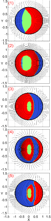
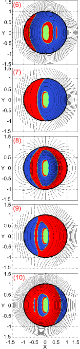
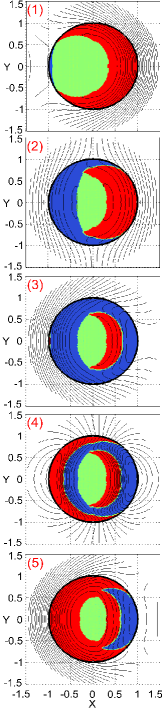
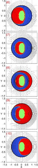
Figure S17: Evolution of the magnetic flux lines and profiles of current with asynchronous oscillating sources $B_{0,y}$ and $I_{tr}$, of amplitudes $B_{\tt{a}}=4$ and $I_{\tt{a}}=0.5$. In the left pane, some of the results for the temporal process displayed in pane (b) of Fig. 6.12 ($B_{0,y}$ has the lower frequency) are shown. Analogously, the results for the pane (c) of Fig. 6.12 ($I_{tr}$ has the lower frequency) are shown at the right pane.

(1)      For asynchronous excitations, the distribution of screening currents in the first peak of the dominant excitation (i.e., that with a longer period), may be strongly different as compared to the attained distributions for the subsequent excitation peaks [Fig. S17, pag. II]. Thus, the first peak of excitation cannot be considered as a steady-state for integrating the AC loss when the integral is reduced to half period of excitation. In other words, the knowledge of the distribution of screening currents in the time elapsed for the second half-period of the dominant excitation is relevant. The latter fact has been experimentally recognized in Ref. [99].

(2)      Whatever electromagnetic excitation carries the double frequency, we have found that, in the AC regime, complex arrays of domains connected by boundary lines with currents switching between $I_{c}$ and $-I_{c}$ appear [see Fig. 6.13 (pag. 6.13) or Fig. S17 (pag. II)].

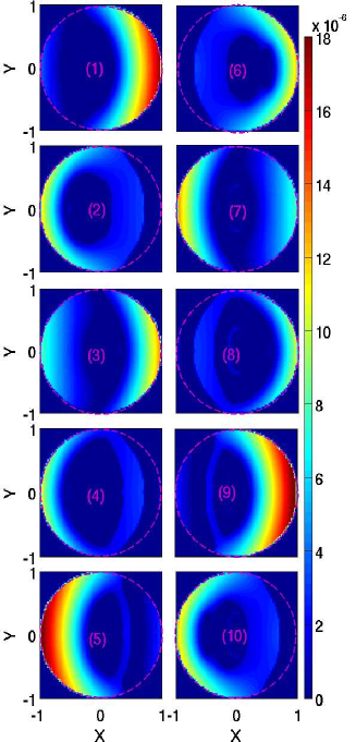
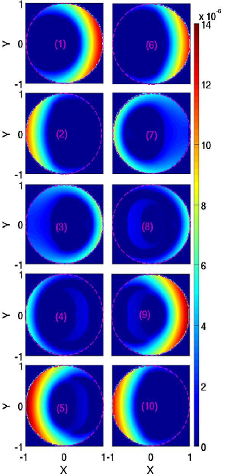
Figure S20: Evolution of the local density of power dissipation E$\cdotp$J for cases with asynchronous AC sources $B_{0,y}$ and $I_{tr}$, according to the current density profiles displayed in Fig. S17.

(3)      Contrary to the strong localization of the local density of power losses observed in cases with synchronous excitations, for asynchronous excitations the active zone with higher heat release is no longer focused at only one side of the superconducting wire [see Fig. 6.13 (pag. 6.13) or Fig. S20 (pag. II)].

(4)      As far as concerns to the magnetic response of the superconducting wire when double frequency effects are incorporated, exotic magnetization loops are predicted [see Fig. 6.14 (pag. 6.14) and Fig. 6.15 (pag. 6.15)]. Outstandingly, for low amplitudes of the transport current, $I_{\tt{a}}$, Bean-like loops may be observed for any of the above mentioned cases. However, as $I_{\tt{a}}$ increases, strongest differences between the magnetization loops arise, and the global behavior is radically different to the synchronous cases.

(5)      A comprehensive analysis of the magnetization curves as a function of the temporal evolution of the electromagnetic excitations has been carried out. Thus, several symmetry conditions for the magnetization loop, when the electromagnetic excitation with double frequency is either $I_{tr}$ or $B_{0}$, concerning to the amplitudes $I_{\tt{a}}$ and $B_{\tt{a}}$ have been illustrated.

(6)      In order to attain the low-pass filtering effect in the temporal evolution of the magnetization curve when $I_{\tt{a}}\rightarrow I_{c}$, it becomes absolutely necessary to assure that both oscillating excitations evolve synchronous in time.

(7)      Accordingly to the different setups in panes (b) and (c) of Fig. 6.12, we have calculated the hysteretic AC loss for several values of $B_{\tt{a}}$ and $I_{\tt{a}}$, when the dominant excitation is either the applied magnetic field, $L_{asynch}^{(b)}$, or the impressed transport current, $L_{asynch}^{(c)}$ [Fig. 6.16, pag. 6.16]. By comparing them with the hysteretic AC loss predicted for the synchronous cases [see also Fig. 6.17, pag. 6.17], we have shown the AC loss may either increase or decrease by double frequency effects when asynchronous excitations are involved. The relative intensities of the excitations $B_{\tt{a}}$ and $I_{\tt{a}}$ play an additional role on this. Then, the big number of possible combinations makes it imperative to have a previous knowledge of the operational environment of the superconducting wire, for attaining valid predictions of the actual AC losses.

Supplementary Material II

• SC wire subjected to an AC transport current
  condition

• SC wire subjected to an AC external magnetic flux

• SC wire subjected to synchronous oscillating
  excitations

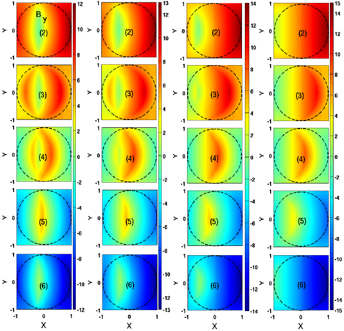
Figure S10: Colormaps for the evolution of the component of magnetic flux density $B_{y}$, corresponding to the current profiles displayed in Fig. S8.

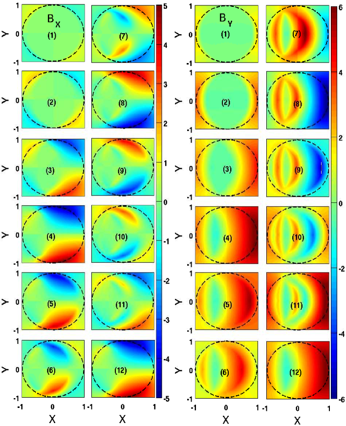
Figure S12: Colormaps for the evolution of the components of magnetix flux density $B_{x}$ (left) and $B_{y}$ (right) for the current density profiles displayed at the left pane of Fig. S11. For $B_{y}$, subplots (3) to (6), and (12), the colormap have to be renormalized to a linear scale of limits 10 and -10.

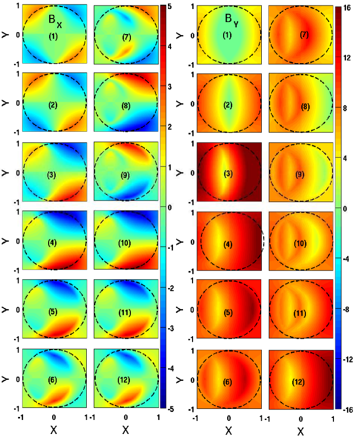
Figure S13: Colormaps for the evolution of the components of magnetix flux density $B_{x}$ (left) and $B_{y}$ (right) for the current density profiles displayed at the rigth pane of Fig. S11.

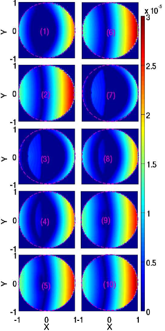
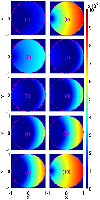
Figure S15: Evolution of the local density of power dissipation E$\cdotp$J for oscillating sources of amplitude $B_{\tt{a}}=8$ and, $I_{\tt{a}}=0.25$ (left pane), and $I_{\tt{a}}=1$ (right pane). Each step has been plotted according to the temporal process depicted in Fig. 6.4, and some of the corresponding flux profiles have been displayed in the left and right columns of Figs. S8- S10. In the right pane, the colormap for subplots (6) and (10) have to be renormalized by a factor of 2.

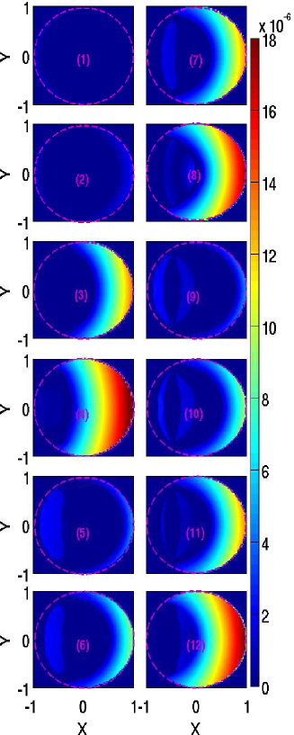
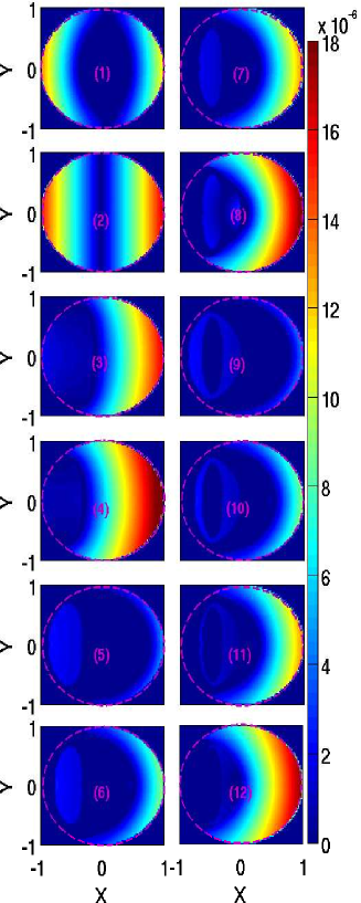
Figure S16: Evolution of the local density of power dissipation E$\cdotp$J for cases with synchronous sources $(B_{0,y},I_{tr})$ and premagnetized superconducting wires with: $B(t^{\prime})=2$ (left pane) and $B(t^{\prime})=8$ (right pane), in correspondence to the profiles of current density displayed in Fig. S11.

• SC wire subjected to asynchronous oscillating
  excitations

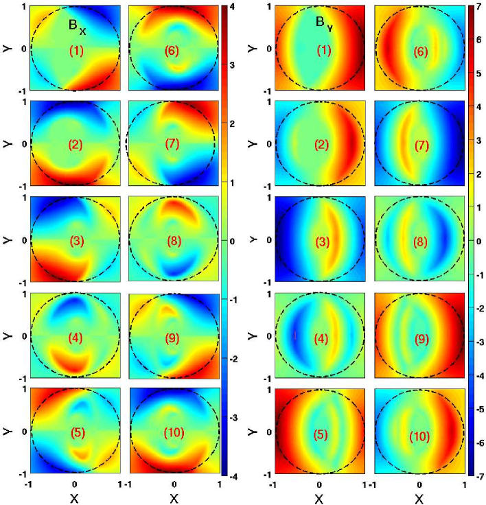
Figure S18: Colormaps for the evolution of the components of magnetix flux density $B_{x}$ (left) and $B_{y}$ (right) for the current density profiles displayed at the left pane of Fig. S17.

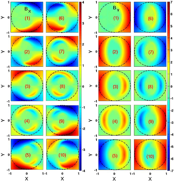
Figure S19: Colormaps for the evolution of the components of magnetix flux density $B_{x}$ (left) and $B_{y}$ (right) for the current density profiles displayed at the right pane of Fig. S17.

Part III Microscopical aspects also analyzed

      Introduction

After one century of the discovery of superconductivity we are still awaiting for a conclusive theory at least beyond normal metals, that are described within the framework of the BCS theory [2]. However, this does not mean that we lack well-established theories to explain some of the experimental facts, despite many of the thermodynamic properties as the high superconducting transition temperature $(T_{c})$ can not be reproduced under a unique scheme. Interestingly, although that the theoretical background behind the understanding of the microscopical aspects involved in the creation of the superconducting state is rather complex, we have found that relatively simple numerical techniques may be used in order to withdraw relevant conclusions from specific experimental data [3, 4, 5].

Our point of interest is the following. In conventional metals, the electron-phonon (E-Ph) coupling mode has long been recognized as the main mechanism involved in the superconducting properties, because the strength of this interaction essentially determines the value of $T_{c}$. However, in the HTSC the experimentally determined $d-$wave pairing in their layered crystal structure with one or more CuO₂ planes per unit cell [6], introduces considerable theoretical complications even when other coupling modes are considered [7]. Fortunately, with the appearance of a new era of analyzers for Angle Resolved Photoemission Spectroscopies (ARPES) with improved resolution both in energy and momentum [8], the controversy on the influence of the anisotropic character of the superconducting gap in the electron properties of HTSC can be directly avoided just by analyzing preferential directions within the $CuO_{2}$ planes or the so-called nodal directions. These directions are basically characterized by a negligible contribution of the superconducting gap along the $(0,0)-(\pi,\pi)$ direction in the Brillouin zone, providing a smart solution if one is merely interested in identifying the energy modes of the quasiparticles involved in the superconducting pairs formation, i.e., in the origin of the coupling mode which binds two electrons (holes) in the formation of Cooper pairs.

In order to understand the relevance of the ARPES technique, we recall that the photoemission process results in both an excited photoelectron and a photohole in the final state. On the one hand, unlike other probes, the ARPES technique has the advantage of momentum resolving, which becomes a useful probe of the related scattering mechanisms contributing to the electrical transport in different materials. We want to note that the single-particle scattering rate measured in ARPES is not identical to the scattering rate measured in transport studies themselves. Nonetheless, direct proportionality between them has been established [9, 10]. On the other hand, one of the most telling manifestations of the E-Ph mode is a mass renormalization of the electronic dispersion at the energy scale associated with the phonons. This renormalization effect is directly observable in the ARPES measurements as a low-energy excitation band in the dispersion curves of photo-emitted electrons, known as kink [11, 12]. In other words, the kink effect can be understood as a well-defined slope change in the electronic energy-momentum dispersion in a similar energy scale ($E_{k}-E_{F}\sim 40-80meV$). This feature, so far universal in the HTSC, has been regarded as a signature of the strength of the boson mechanism which causes the pair formation in the superconducting state. In fact, all the interactions of the electrons which are responsible for the unusual normal and superconducting properties of cuprates are believed to be represented in this anomaly [13]. This has prompted an intense debate about the nature of the coupling mode involved in the density of low-energy electronic excited states in the momentum-energy space, and its influence on the emergence of the superconducting state [3, 4, 5, 11, 12, 13, 14, 15, 16, 17, 18, 19, 20, 21, 22, 23, 24, 25, 26, 27, 28, 29].

In an effort to clarify the influence of the phonon coupling mode (either weak or strong), we have analyzed the influence of the E-Ph interaction on the electronic dispersion relations for several cuprate compounds. A full discussion of the ARPES technique, as well as a detailed description of the strong correlations theory which have been used to reproduce the nodal kink effect in HTSC is more appropriately reserved for specialized texts in photoemission spectroscopies and many body theories [see e.g., Refs. [30, 31, 32, 33, 34, 35]]. However, we can, in a brief way, introduce the basic concepts of the E-Ph coupling theory for photoemission spectroscopies, and give a thorough interpretation of the influence of this boson coupling mode on the momentum distribution-curves (MDC) measured by ARPES (chapter 7), and finally argue about how strong can be considered the phonon coupling mode from the analysis of the predicted values for $T_{c}$, the ratio gap $2\Delta_{0}/k_{B}T_{c}$, and the zero temperature gap $\Delta_{0}$ (chapter 8).

On the one hand, in chapter 7 our analysis shows a remarkable agreement between theory and experiment for different samples and at different doping levels. Universal effects such as the nodal kinks at low energies are theoretically reproduced, emphasizing the necessary distinction between the general electron mass-enhancement parameter $\lambda^{*}$and the conventional electron-phonon coupling parameter $\lambda$. On the other hand, in chapter 8 a thorough analysis of the superconducting thermodynamic quantities and the Coulomb effects based on different approaches will reveal as, contrary to the predictions for LSCO samples, in more anisotropic materials as Bi2212 and Y123 families, it seems unavoidable to consider additional coupling modes in order to justify their high critical temperatures.

Chapter 7 E-Ph Theory And The Nodal Kink Effect In HTSC

The photoemission process formally measures a complicated nonlinear response function. However, it is helpful to notice that the analysis of the optical excitation of the electron in the bulk greatly simplifies within the “sudden approximation” [36, 37]. It means that the photoemission process is supposed to occur suddenly, with no post-collisional interaction between the photoelectron and the system left behind [38]. In particular, it is assumed that the excited state of the sample (created by the ejection of the photo-electron) does not relax in the time it takes for the photo-electron to reach the detector [13]. It can be shown that within the sudden approximation using Fermi’s Golden Rule for the transition rate, the measured photo-current density is basically proportional to the spectral function of the occupied electronic states in the solid, i.e.: $J_{\bf k}\propto A_{\bf k}(E_{k})$. Eventually, and validated by whether or not the spectra can be understood in terms of well defined peaks representing poles in the spectral function, one may connect $A_{\bf k}(E_{k})$ to the quasiparticle Green’s function $G(\textbf{k},E)=1/(E_{k}-\Sigma_{k}(E_{k})-\varepsilon_{k})$, with $\Sigma_{k}(E_{k})$ defining the electronic self-energy and $\varepsilon_{k}$ the bare band dispersion. In fact, customarily the inversion method for the experimental data in ARPES is based upon the so called sudden approximation trough the relation $A(\textbf{k},\omega)=-(1/\pi)$Im$G(\textbf{k},\omega+i0^{+})$. Beyond the sudden approximation, one would have to take into account the screening of the photoelectron by the rest of the system, and the photoemission process could be described by the generalized golden rule formula, i.e, a three-particle correlation function [37]. However, for our purposes, it is important mention the evidence that the sudden approximation is justified for the cuprate superconductors even at low photon energies [36, 39]. In the end, the suitability of the approximations invoked, will be justified by the agreement between the theory and the experimental observations.

In the diagrammatic language, the above approach can be reduced to calculate the quasiparticle self energy $\Sigma_{k}$ within the framework of the Fermi-liquid theory, where electron-like quasiparticles populate bands in the energy-momentum space up to the cut-off at the Fermi energy. In the case of normal metals, this sophisticated description was firstly introduced by Migdal [40] who showed that the small parameter $N(0)\theta_{D}$ allows to consider the higher order corrections negligible, assuming that the density of states $N(\varepsilon)$ is approximately a constant $N(0)$ over the interval $(-\theta_{D},\theta_{D})$ around the Fermi level $\varepsilon_{F}$. Here, $\theta_{D}$ is the so-called Debye energy.

However, in the case of superconductors, the theory requires to incorporate the Cooper-pairs condensation through a bosonic coupling function assuming that both the electronic and the bosonic spectrum are possible to obtain from inelastic neutron scattering (INS) measurements, X-Ray scattering (XRS) experiments, tunneling experiments, or ab-initio calculations of the electronic band structure. This complex picture can be understood, in general terms, from the so-called Eliashberg theory [41], and the works by Nambu [42], Schrieffer [43], and Morel and Anderson [44]. In this scenario, the boson spectrum is directly associated to the lattice vibration (phonons) as the binding mechanism for the Cooper-pairs formation. Nevertheless, this theory also has been often considered as the base of another possible mechanisms with a magnetic origin [9, 45, 46, 47, 48, 49, 50, 51, 52, 53]. As there is not any argument which allows to validate this assumption, onwards, we will refer only to phonons as the boson coupling mechanism.

In order to support our “phononic choice” we want to recall that the absence of the magnetic-resonance mode in LSCO ($La_{2-x}Sr_{x}CuO_{4}$) [16], Bi2212 ($Bi_{2}Sr_{2}CaCu_{2}O_{8+x}$) over-doped (x=0.23) [54], and its appearance only below $T_{c}$ in some cuprates (e.g., Bi2201 [55]) are not consistent with the universality of the kink effect. Moreover, recent studies on electron doped systems [28, 56, 57, 58] have shown that the intensity of the magnetic resonance mode is seemingly weak in comparison with the phonon mode to be considered as the cause of the strong electron energy dispersion measured by ARPES.

In the forthcoming paragraphs, and relying on a solid theoretical basis that is introduced within the supplementary material section for the reader’s sake, we present our analysis of available experimental data.

  7.1 Basic statements for the E-Ph coupling

As a manifestation of the electron-phonon coupling interaction one can introduce the mass renormalization of the electronic dispersion at the energy scale associated with the phonons. This may be technically defined from the real part of the electron self energy as a mass-enhancement parameter $\lambda^{*}$ [59] given by,

$$\lambda_{k}^{*}\equiv\left.-\partial_{\omega}\Sigma_{1}\right|_{\omega=0}\,.$$ (7.1)

Although related (as it will be later clarified), $\lambda^{*}$ must not be interpreted as the strength of the E-Ph interaction which is estimated from the so-called boson coupling parameter $\lambda$. This dimensionless parameter is commonly defined in terms of the electron-phonon spectral density as

$$\lambda\equiv 2\int_{0}^{\infty}d\nu\,\frac{\alpha^{2}F(\nu)}{\nu}\,,$$ (7.2)

and it is customarily related to the superconducting transition temperature. In fact, as we have argued in Ref. [3], equality would just be warranted at very low temperatures, and ensuring that the spectral density measured from the experiments is fully satisfying the ME approach for the Feynman diagram of lowest order for the E-Ph interaction [see Fig. SIII-I (pag. III), in the section of supplementary material III].

Hence, taking into consideration the inherent existence of phonons in the HTSC, we have evaluated the electron spectral densities for $La_{2-x}Sr_{x}CuO_{4}$ (LSCO), $Bi_{2}Sr_{2}CaCu_{2}O_{8+x}$ (Bi2212), and $YBa_{2}Cu_{3}O_{6+x}$ (Y123), in the flat model of Ref. [60] as well as by solving the isotropic Eliashberg equations on the Matsubara frequencies. The structure of these spectral densities is restricted to the isotropic nodal direction under the assumption that $\alpha^{2}F(\nu)=G(\nu)\times C$, with C an adjustable constant and $G(\nu)$ the generalized phonon density of states extracted from the inelastic neutron scattering experiments [60]. Our results are shown in Fig. 7.1 (Shiina’s lines). In addition, other reproducible methods to calculate the E-Ph spectral density have been taken into consideration. Specifically, we mean the simple method by Islam & Islam [61] (Islam’s lines), and the method by Gonnelli et al. [62], the last only referred for the Bi2212 family (Gonnelli’s line). The method of Refs. [60] & [61] is based on the INS experimental data by Renker et al. [63, 64, 65], and the method in Ref. [62] is based on the tunneling data reported in Refs. [66, 67].

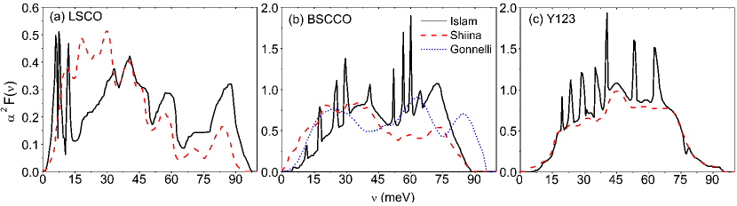
Figure 7.1: E-Ph spectral density $\alpha^{2}\textit{F}(\nu)$ for (a) $La_{2-x}Sr_{x}CuO_{4}$ (LSCO), (b) $Bi_{2}Sr_{2}CaCu_{2}O_{8+x}$ (Bi2212), and (c) $YBa_{2}Cu_{3}O_{6+x}$ (Y123), determined by different methods. The solid lines correspond to the method in Ref. [61], dashed lines to the method in Ref. [60], and the dotted line in (b) corresponds to the method of Ref. [62].

On the other hand, as it is shown in the supplementary material section, and after some simple mathematical manipulations, the E-Ph self energy ($\Sigma$) can be rewritten within the ME approach as a complex function of the form:

$$\Sigma(\textbf{k},i\omega)=\int_{0}^{\infty}d\nu\alpha^{2}F(\textbf{k},\nu)\left\{-2\pi\leavevmode\nobreak\ i\left[N(\nu)+\frac{1}{2}\right]+\Upsilon(\nu,\omega,T)\right\}\,,$$ (7.3)

where the function $\Upsilon(\nu,\omega,T)$ is defined in terms of the so-called digamma functions $\psi(z)$,

$$\Upsilon(\nu,\omega,T)=\psi\left(\frac{1}{2}+i\frac{\nu-\omega}{2\pi T}\right)-\psi\left(\frac{1}{2}-i\frac{\nu+\omega}{2\pi T}\right)\,.$$ (7.4)

At this point, is useful recall that the bare band energy $\varepsilon_{\textbf{k}}$ is related to the dressed band energy $E_{\textbf{k}}$ by

$$E_{\textbf{k}}=\varepsilon_{\textbf{k}}+Re\Sigma(E_{k})\,.$$ (7.5)

Whereas the direct extraction of the self-energy from experiments appears to be troublesome because the underlying band structure of the bare electrons is a priori unknown, a theoretical determination of the bare band structure and its relation to the full energy renormalization effects observed in the experiments seems much more attractive. In this sense, the nodal ARPES spectra are of great importance to check the validity of the quasiparticle concept discussed above, and also for understanding the nature of the involved interactions.

  7.2 E-Ph model for the nodal kink effect

Let me make some final remarks before moving onto the application of the above ideas to the analysis of the nodal kink effect in the ARPES data. On the one hand, is to be mentioned, that the energy distribution- and momentum distribution-curves (EDC - MDC) are the two most popular ways for analyzing photoemission data. The dichotomy between the MDC- and EDC-derived bands from the same data raises critical questions about its origin and also about which one represents the intrinsic band structure. In this sense, we want to recall that at the larger bandwidth along the nodal direction, the MDC method can be reliably used to extract high quality data of dispersion in searching for fine structure. It has also been shown theoretically that this approach is reasonable in spite of the momentum-dependent coupling [14]. In a typical Fermi liquid picture, the MDC- and EDC-derived dispersions are identical. Moreover, in an electron-boson coupling system the lower and higher energy regions of the MDC- and EDC-derived dispersions are still consistent, except right over the kink region [24]. On the other hand, recalling that the bare electron band energy $\varepsilon_{k}$ is not directly available from the experiments. Instead, the electron momentum dispersion curve $E_{k}(k-k_{F})$ may be measured. Below, we show that the good agreement between our theoretical data and the experimental facts supports this general picture.

As the kink effect is a common feature of the whole set of HTSC families i.e., it is observable regardless of the doping level or the temperature at which the measurement is performed, the only possible scenario seems to be the coupling of quasiparticle with phonons. Thus, we have noted that the relation between the dressed and bare energies is a central property as related to the kink structure. The key issue seems to be the existence of an energy scale (in the range of 40-80 meV).

We have proposed an integral equation formalism based on the combination of Eqs. 7.2 – 7.5 from which, one can consider that $\varepsilon_{k}$ implicitly depends on $E_{k}$ through the boson coupling parameter $\lambda$ [3]. In other words, Eq. 7.2 acts as an integral constraint, through the definition of $\lambda$. Thus, based on an interpolation scheme between the numerical behavior of the dressed energy band and the experimental data, one can introduce a universal dispersion relation which allows to reproduce in a quite general scheme the nodal dispersions close to the Fermi level [3, 4, 5]. As a central result, we have encountered that the practical totality of data are accurately reproduced by a universal linear dispersion relation of the kind

$${k}-{k}_{F}=\frac{\varepsilon_{k}}{v_{F_{<}}}\left(1-\delta\lambda\right)\,,$$ (7.6)

with $v_{F_{<}}$ the Fermi velocity at low-energies, and $\varpi$ as the (only) “free” parameter required for incorporating the specific renormalization for each superconductor. From the physical point of view, our empirical ansatz [Eq.(7.6)] may interpreted as follows. Into the ME approach, the involved quantities are not far from their values at the Fermi level, and one can start with $\varepsilon_{k}$ replaced by $E_{k}-\Sigma_{1}(E_{k})$, i.e.,

$$E_{k}-\Sigma_{1}(E_{k})=\left({k}-{k}_{F}\right)v_{F_{<}}\left(1-\delta\lambda\right)^{-1}\,.$$ (7.7)

Then, taking derivatives with respect to $E_{k}$ and evaluating them for $E_{k}\to 0$, one gets

$$1+\lambda^{*}=\left.\frac{\partial(k-k_{F})}{\partial E_{k}}\right|_{E_{k}=0}v_{F<}(1-\delta\lambda)^{-1}\,,$$ (7.8)

and recalling that $v_{F<}$ is obtained as the slope of the lower part of the momentum dispersion curve, this equation leads to $1+\lambda^{*}=(1-\delta\lambda)^{-1}$. Thus, a physical interpretation of the fit parameter $\delta$ is straightforwardly obtained from the analytical relation

$$\delta=\frac{\lambda^{*}}{\lambda(1+\lambda^{*})}\,.$$ (7.9)

To the lowest order, the dimensionless parameter $\delta$ is basically the ratio between the defined mass-enhancement and phonon-coupling parameters $\delta\approx\lambda^{*}/\lambda$. Outstandingly, this fact reassembles the differences obtained by tight-binding Hamiltonian models [68, 69] and the “density-functional” band theories [27, 70] appealing to the differences between $\lambda$ and $\lambda^{*}$. To understand these differences, recall that, in principle, the density-functional theory [71] gives a correct ground-state energy, but the bands do not necessarily fit the quasi-particle band structure used to describe low-lying excitations.

  7.3 Numerical procedure and results

In order to reproduce the experimental results, our numerical program is as follows:

1. $v_{F_{<}}$ is determined from the momentum dispersion curve in the ARPES measurements [$\sim$ 1.4 eV$\cdot$Å - 2.2 eV$\cdot$Å],

2. To determine $\delta$, we calculate the so called logarithmic frequency $\omega_{\rm log}$ as introduced by Allen and Dynes [77],

   $$\omega_{\rm log}\equiv exp\left\{\frac{2}{\lambda}\int_{0}^{\infty}\ln(\nu)[{\alpha^{2}F(\nu)}/{\nu}]d\nu\right\}\,.$$ (7.10)

   This constant frequency (properly defining the corresponding spectral densities $\alpha^{2}F(\nu)$ for each $\lambda$) is introduced only for scaling purposes $(\delta=\varpi/\omega_{\rm log})$. Thus, we achieve a reduction in the scattering of numerical values when dealing with different samples. In this sense, $\varpi$ is a mere mathematical instrument. For the spectral densities shown in Fig. 7.1 we get $\omega_{\rm log}^{LSCO}\simeq 16.1455\,meV$, $\omega_{\rm log}^{Y123}\simeq 35.5900\,meV$ and $\omega_{\rm log}^{Bi2212}\simeq 33.8984\,meV$, respectively.

3. $\varepsilon_{k}$ is numerically determined from the relation $E_{k}=\varepsilon_{k}+Re\{\Sigma(E_{k})\}$, where the digamma functions are simply subroutines of our code.

4. Finally, correlation between theory and experiment is established by the application of Eq. (7.6). The best fit with the experimental curves has been obtained for $\delta=0.185$ in LSCO, $\delta=0.354$ in Bi2212, and $delta=0.365$ in Y123 families, respectively.

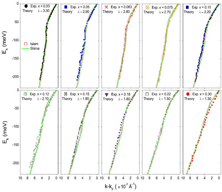
Figure 7.2: The renormalized electron quasiparticle energy dispersion $E_{k}$ as a function of the momentum $k-k_{F}$ for several samples of $\texttt{La}_{2-x}\texttt{Sr}_{x}\texttt{CuO}_{4}$, measured along the (0,0)-($\pi$,$\pi$) nodal direction at a temperature of 20 K. The doping level $x$ ranges between 0.03 (top left) up to 0.30 (bottom right). The experimental data (symbols) are taken from Ref. [12] and the theoretical curves have been obtained using the spectral densities of Islam & Islam [Ref. [61]] (open squares), and Shiina & Nakamura (solid lines)[60].

In Fig. 7.2 we show the results found in LSCO covering the doping range ($0<x\leq 0.3$). Remarkably, within this range, the hole concentration in the $CuO_{2}$ plane is well controlled by the $Sr$ content and a small oxygen non-stoichiometry, where the physical properties span over the insulating, superconducting, and overdoped non-superconducting metal behavior. Superconducting transition temperatures $T_{c}$ in the interval of 30-40K have been observed in Refs. [6, 72, 73]. For the application of Eq. (7.6), we have considered $v_{F_{<}}=2eV\cdot$Å as related to the experimental results of Refs. [11, 12, 13, 16]. The best fit of the whole set of experimental data has been obtained for $\delta=0.185$, and the derived $\lambda^{*}$ values are shown in Table 7.1. For comparison, recall that values of “$\lambda=2-2.5$” in the range $0.2>x>0.1$ were reported in the Ref. [68] by Weber. In that case, these values were obtained within the framework of the nonorthogonal-tight-binding theory of lattice dynamics, based on the energy band results of Mattheiss [74]. It must be emphasized that in both cases (Ref. [68] & Refs [3, 4]), $\lambda$ was obtained in agreement with the observed $T_{c}$ values in LSCO. Moderate discrepancies between the predictions of our model and the analysis of Refs. [68] & [69] may be ascribed to some uncertainty in the experimental spectral densities.

On the other hand, we have taken advantage of the widespread availability of experimental information in LSCO [11] and our numerical method, to describe the evolution of the E-Ph coupling parameter $\lambda$ as a function of the doping level. It can be fitted to the simple expression

$$\lambda=2\tilde{\omega}exp(-\frac{\tilde{\omega}}{\delta}x)+1\,,$$ (7.11)

within a precision factor of $\sim 95$% (Fig. 7.3). Here, $\tilde{\omega}$ defines the ratio between the phonon characteristic energies introduced by McMillan [75],

$$\omega_{\rm 1}=(2/\lambda)\int_{0}^{\infty}\alpha^{2}F(\nu)d\nu\equiv(2/\lambda)S\,,$$ (7.12)

and the logarithmic frequency $\omega_{\rm log}$ [Eq. (7.10)]. In this case, we get $\omega_{\rm log}^{LSCO}\simeq 16.1455\,meV$ and $\omega_{1}^{LSCO}\simeq 25.2627\,meV$.

Table 7.1: Values of the E-Ph coupling parameter $\lambda$ and the corresponding mass-enhancement parameter $\lambda^{*}$ obtained from the analysis of ARPES data at several doping levels ($x$) of $La_{2-x}Sr_{x}CuO_{4}$, $Bi_{2}Sr_{2}CaCu_{2}O_{8+x}$. $\lambda^{*}$ has been obtained by means of Eq. (7.6) to the lowest order $\lambda^{*}\approx\delta\lambda$. The predicted superconducting transition temperatures $T_{c}$ are also shown. Our results are presented in contrast with other models available in the literature.

$La_{2-x}Sr_{x}CuO_{4}$	(LSCO).			$\delta=0.85$
$x$	Ref.	$\lambda$	$\lambda^{*}$	$T_{c}(\lambda)$ [K]
0.03		3.30	0.61	–
0.05		2.90	0.54	–
0.063		2.80	0.52	–
0.075		2.70	0.50	–
0.10		2.20	0.41	42.10
0.12		2.10	0.39	40.77
0.15		1.90	0.35	37.83
0.18		1.80	0.33	36.19
0.22		1.50	0.28	30.47
0.30		1.30	0.24	–
0.1-0.2	[68]	2-2.5	–	30–40
–	[60]	1.78	–	40.6
0.15	[27]	1–1.32	0.14–0.22	–
0.22	[27]	0.75–0.99	0.14–0.20	–

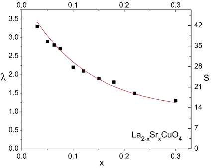
Figure 7.3: Evolution of the E-Ph coupling parameter $\lambda$ as a function of the dopant content in LSCO. The $\lambda$-values have been obtained from our best fit with the nodal kink dispersion (black squares) shown in Fig. 7.2. Correspondingly, the evolution of the area $S$ as a function of the dopant content is also shown (right scale).

Table 7.2: Same as Table 7.1 but for $Bi_{2}Sr_{2}CaCu_{2}O_{8+x}$.

$Bi_{2}Sr_{2}CaCu_{2}O_{8+x}$	(Bi2212).			$\delta=0.354$
$x$	Ref.	$\lambda$	$\lambda^{*}$	$T_{c}(\lambda)$ [K]
0.12		2.15	0.76	64.81
0.16		1.33	0.47	42.45
0.21		0.85	0.30	19.93
–	[60]	3.28	–	85
–		3.28	1.16	81.66
–	[62]	3.34	1.05	93
–		3.34	1.18	82.40
0.16	[17]	$\sim 1.28$	$\sim 0.43$	–

We want to clarify that, although Eq. (7.11) can be considered as a useful relation between the physical and chemical properties of LSCO, the shaping of other HTSC families by similar expressions cannot be guaranteed.

In Table 7.2 and Fig. 7.4, we display the results found for the available experimental data in Bi2212 samples. In this case, the theoretical curves for $E_{k}(k-k_{F})$ have been predicted by our interpolation method for the under-doped (UD70) “$x=0.12$, $T_{c}\approx 70K$”, optimally doped (0PD90) “$x=0.16$, $T_{c}\approx 90K$”, and over-doped (OVD58) “$x=0.21$, $T_{c}\approx 58K$” samples, having use of the spectral densities of Fig. 7.1. The experimental data were taken from the work by Johnson et al. [22] with $v_{F_{<}}=1.6eV\cdot$Å as a value consistent with the experimental results of Refs. [11, 15, 17, 22]. The best fit with experimental data has been found for $\delta=0.354$. We show that, regardless the method used for obtaining the E-Ph spectral density, the same conclusions can be achieved.

Table 7.3: Same as Table 7.1 but for $YBa_{2}Cu_{3}O_{6+x}$.

$YBa_{2}Cu_{3}O_{6+x}$	(Y123).			$\delta=0.365$
$x$	Ref.	$\lambda$	$\lambda^{*}$	$T_{c}(\lambda)$ [K]
0.4		0.80	0.29	17.51
0.6		0.65	0.24	9.82
0.85		0.50	0.18	3.39
–	[60]	$\sim$3.4	–	91
–		3.45	1.26	84.19
–	[69]	$\sim$0.5	–	$\sim$3
–	[69]	$\sim$1.3	–	$\sim$30
–		1.30	0.47	36.43
–	[70]	–	0.18 - 0.22	–
–		0.49 - 0.60	0.18 - 0.22	$\sim$3.0–6.6

Finally, in Table 7.3 and Fig. 7.5 we show the results found for Y123 with the following dopant levels: Under-Doped 35 “$x=0.4$, $T_{c}\approx 35K$” (UD35), Under-Doped 61 “$x=0.6$, $T_{c}\approx 61K$” (UD61), and Over-Doped 90 “$x=0.85$, $T_{c}\approx 90K$” (OVD90). The experimental data were taken from the work by Borisenko et al. [23]. To our knowledge, no more experimental evidence of kinks in the nodal direction is available for this material. The value $v_{F_{<}}=1.63eV\cdot$Å has been used for consistency with the experimental results reported by those authors. The best fitting between the experimental data and our model has been found with the value $\delta=0.365$. It must be noted that the appearance of a second kink in the underdoped case may not be allocated with the simple assumptions of our model. Nevertheless, although this effect could be explained either by introducing high perturbation orders beyond the ME approach or introducing a renormalization factor for the electronic band structure, the range of energies for the E-Ph spectral density does not seems provide a physically admissible explanation.

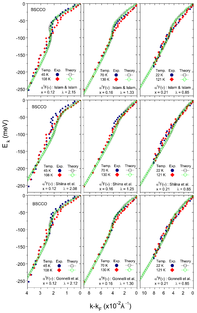
Figure 7.4: Same as in Fig. 7.2 but in samples of Bi2212. The experimental data for the normal state (full diamond) and superconducting state (full circle) both have been taken from the Ref. [22]. The theoretical curves (lines -diamond, or -circles) have been obtained from our interpolation method [Eq. (7.6)] according to the best fit values for the E-Ph coupling parameter $\lambda$, and the spectral densities of Islam & Islam [61] (top), Shiina & Nakamura [60] (middle), and Gonnelli et al. [66] (bottom). The different plots correspond to the doping levels of Bi2212: under-doped “x=0.12” (left), optimally doped “x=0.16” (center), and over-doped “x=0.21” (right) respectively.

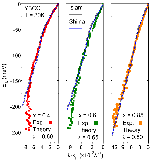
Figure 7.5: Same as in Fig. 7.2 but in samples of Y123 with (left to right): $x=0.4$ (underdoped), $x=0.6$ (underdoped), and $x=0.85$ (overdoped). The solid squares correspond to the experimental data of Ref. [23]. The theoretical curves have been obtained using the spectral densities of Islam & Islam [Ref. [61]] (open squares), and Shiina & Nakamura [Ref. [60]] (solid line). All curves have been obtained at 30K.

Chapter 8 Is it necessary to go beyond the E-Ph mode?

According to the previous chapter, the results for optimally doped Bi2212 (OPD90, $x=0.16$) and over doped Bi2212 (OVD85, $x=0.21$) samples (Fig. 7.4), with measured $T_{c}=90K$ and $85K$ respectively, have revealed that the influence of the E-Ph coupling mechanism is seemingly weak in spite of the kink effect is reproduced for the whole energy spectrum. On the other hand, the discrepancies become even larger when the thermodynamic properties for Y123 samples are analyzed.

🍂     To address the question:

In order to answer Is it necessary to go beyond the E-Ph coupling mode for the superconducting pairs formation?, we can a priori consider that some of the E-Ph spectral densities of Fig. 7.1 will allow explain the high $T_{c}$ values and the zero temperature gap $\Delta_{0}$ reported in the literature. From this point of view, several approaches can be argued for each one of the materials. For example, in Fig. 8.1 we show our results for $T_{c}$, the ratio gap $2\Delta_{0}/k_{B}T_{c}$ and the zero temperature gap $\Delta_{0}$ for the different HTSC families analyzed in the above chapter. The different curves have been obtained from the point of view of three different approaches

1. The celebrated McMillan’s equation [75],

   $$T_{c}=\frac{\omega_{1}}{1.2}exp\left[-1.04\frac{1+\lambda}{\lambda-\mu^{*}(1+0.62\lambda)}\right]\,,$$ (8.1)

   with $\mu^{*}$ the so-called Coulomb pseudopotential.

2. The refined formula by Allen and Dynes [77], which is obtained by replacing $\omega_{1}$ [Eq. (7.12)] in Eq. (8.1) by the so called logarithmic frequency $\omega_{log}$ [see Eq. (7.10)].

   For the HTSC families considered along this section, and the different spectral densities of Fig 8.1, we get $\omega_{\rm log}^{LSCO}\simeq 16\,meV$, $\omega_{1}^{LSCO}\simeq 25\,meV$, $\omega_{\rm log}^{Bi2212}\simeq 33\,meV$, $\omega_{1}^{Bi2212}\simeq 39\,meV$, $\omega_{\rm log}^{Y123}\simeq 35\,meV$, and $\omega_{1}^{Y123}\simeq 39\,meV$.

3. Finally, the less conventional Kresin’s formula [78],

   $$T_{c}=0.25\;\varpi\;exp\left(\frac{2}{\lambda_{eff}}-1\right)^{-1/2}\;,$$ (8.2)

   where $\varpi=[(2/\lambda)\int_{0}^{\infty}\nu\alpha^{2}F(\nu)d\nu]^{1/2}$ and $\lambda_{eff}=(\lambda-\mu^{*})[1+2\mu^{*}+(3/2)\lambda\mu^{*}exp(-0.28\lambda)]$.

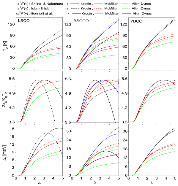
Figure 8.1: Plots of the critical temperatures $T_{c}$ (top), the ratio gap $2\Delta_{0}/k_{B}T_{c}$ (middle) and the gap $\Delta_{0}$ (bottom) for LSCO, Bi2212 and Y123, all of them represented as functions of the E-Ph coupling parameter $\lambda$ obtained from the E-Ph spectral densities shown in Figure 8.1. We have used three different approaches: the McMillan’s formula [75], the Allen-Dynes formula [77], and the Kresin’s formula [78].

In all calculations, the Coulomb’s pseudopotencial was given by a typical value, $\mu^{*}=0.13$ [33]. We have to be mention that is essential to be aware that there is no a small parameter that enables a satisfactory perturbation theory to be constructed for the Coulomb interaction between electrons. Thus, Coulomb contributions to the electron self energy $\Sigma$ introduced in chapter 7 cannot be reliably calculated [77]. Fortunately this is not a serious problem in superconductivity because a reasonable assumption is to consider that the large Coulomb effects for the normal state are already included in the electronic bare band structure $\varepsilon_{k}$. The remaining off-diagonal terms of the superconducting components of the Coulomb self-energy turn out to have only a small effect on superconductivity, which is treated phenomenologically [33].

Is to be noticed that the high values of the critical temperatures strongly depend on the approximation invoked, and (in some cases) on the inversion method for the boson coupling spectral density. Thus, we argue that the critical temperature $T_{c}$ should not be considered as a fit parameter for adjusting the theory, i.e.: one should not predict $\lambda$ from the approximate $T_{c}$ formulas and then use it for calculating the electron self-energy. As a proof of this, we recall that although attractive, this idea has led to underestimates the phonon contribution to the photoemission kink in HTSC [27, 70].

To our knowledge, the most suitable way for determining the influence of an interaction mechanism in the pair formation for HTSC could be (i) evaluate the strength of the boson coupling mode from the electron renormalization effects and then (ii) solve the Eliashberg equations for the superconducting $T_{c}$, or have use of semiempirical approaches as the introduced before. From such analysis, we conclude that the consideration of the E-Ph interaction in LSCO strongly suggests that the high $T_{c}$ values can be caused by the conventional coupling to phonons (see table 7.1). However, for the Bi2212 and Y123 samples the obtained results are not so encouraging as they are for the LSCO family (see tables 7.2 & 7.3).

On the one hand, we have noticed that the obtained critical temperatures for Bi2212-UD70 in the framework of the spectral densities of Islam & Islam [$T_{c}^{Kresin}(\lambda=2.15)=70.0K$ and $T_{c}^{McMillan}(\lambda=2.15)=64.81K$], and Gonnelli et al. [$T_{c}^{Kresin}(\lambda=2.15)=67.06K$ and $T_{c}^{McMillan}(\lambda=2.15)=58.19K$], are in some sense, good estimations for the experimental values of $T_{c}$. However, from the method by Shiina & Nakamura [60], and the framework of the Allen & Dynes formula [77], a strong reduction of $T_{c}$ ($\sim 40\%$) can be found. This can be interpreted as a first signal about the need of considering additional perturbation mechanisms into the matrix elements of the Eliashberg equations, or perhaps, and in an optimistic way for the phonon hypothesis, this fact could be revealing that the flat model used in Ref. [60] is not consistent with the experimental facts of this kind of material.

On the other hand, regarding the Bi2212-OPD90 and Bi2212-OVD85 samples, independently of the inversion method used for the E-Ph spectral density (Fig. 7.1), the maximal values for $\lambda$ which are able to reproduce the kink structure ($\lambda\simeq 1.3$ and $\lambda\simeq 0.85$ respectively), both underestimate the experimental critical temperatures in about $50\%$. The disagreement can be even higher ($\sim 80\%$) if we consider the results for Y123 samples (see Fig. 7.5 & Table 7.3). However, before moving on thinking in the necessity of additional boson coupling mechanisms, is necessary to revalidate the influence of the Coulomb effects along the framework of the different invoked approaches.

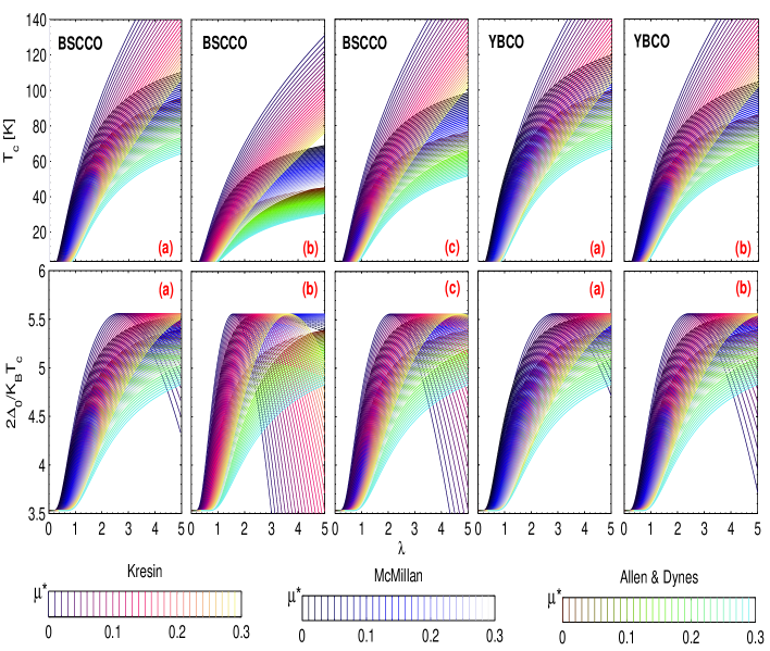
Figure 8.2: Plots of the critical temperatures $T_{c}$ (top), and the ratio gap $2\Delta_{0}/k_{B}T_{c}$ for Bi2212 and Y123 samples, as functions of the E-Ph coupling parameter $\lambda$ and the Coulomb pseudopotential $\mu^{*}$. $\lambda$ has been determined from the spectral densities of: (a) Islam & Islam [61], (b) Shiina & Nakamura [60], and (c) Gonnelli et al. [62]. Three different approximations are shown: the Kresin’s formula [78], the McMillan’s formula [75], and the Allen-Dynes formula [77].

Assuming that the Coulomb effects are almost negligible for the renormalized energy of the electronic quasiparticles participating in the superconducting pairs formation, a remarkable enhancement of the thermodynamic properties could be expected (Fig. 8.2). For example, taking $\mu^{*}=0.001$ rather than the conventional $\mu^{*}=0.13$, and assuming the most favorable scenario for the phonon hypothesis, i.e.: (i) determine the E-Ph spectral density from the methods by Islam & Islam (Ref. [61]), and/or Gonnelli et al. (Ref. [62]), (ii) use of the empirical Kresin’s formula to determine $T_{c}$ (see Fig. 8.2), and (iii) check if it is possible to reproduce the renormalization effects of the scattered quasiparticles along the nodal direction by ARPES measurements; the maximal influence of the E-Ph mechanism for the families of Bi2212 and Y123 can be estimated. For Bi2212-OPD90, we have obtained $\lambda_{Islam}(T_{c}^{Kresin}=91K)\simeq 1.82$ and $\lambda_{Gonnelli}(T_{c}^{Kresin}=91K)\simeq 1.93$, with the renormalization parameters for the ARPES “bare” dispersion $\delta=0.264$ and $\delta=0.248$, respectively. Regarding to Bi2212-OVD58, the obtained E-Ph coupling parameters are: $\lambda_{Islam}(T_{c}^{Kresin}=58K)\simeq 1.12$ and $\lambda_{Gonnelli}(T_{c}^{Kresin}=58K)\simeq 1.17$, for the same $\delta$ values above considered. Along this line, we have observed a widening of the kink effect which can be only explained by the existence of at least one additional perturbation mechanism reducing the momentum of the dispersed quasiparticles (see Fig. 8.3).

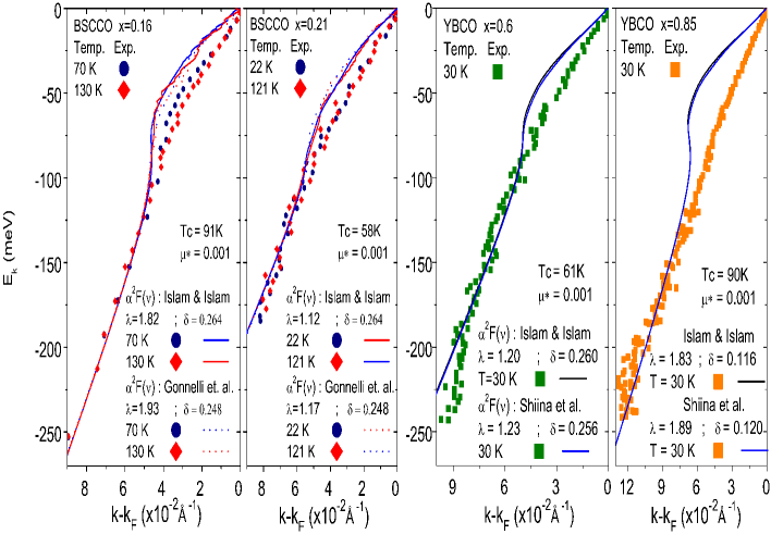
Figure 8.3: The renormalized energy $E_{k}$ as a function of the momentum $k-k_{F}$ under the assumption that the nodal dispersion is a consequence of the E-Ph coupling mode and the Coulomb effects are completely contained in the bare energies. Then, we assume the very weak Coulomb pseudopotential $\mu^{*}=0.001$ within the more favourable approximation for the calculus of $T_{c}$ and the phonon hypothesis, i.e. the Kresin Formula and the E-Ph spectral density $\alpha^{2}\emph{F}(\omega)$ obtained by the methods of Refs. [61, 66] in Bi2212 cases, and Refs. [61, 60] in Y123 cases.

On the other hand, regarding the Y123 samples, the effect of reducing the Coulomb pseudopotential shows that the expected values for $T_{c}$ in Y123-UD35 can be explained under any of the aforementioned formulas. In detail, for $\lambda=0.80$ (see Fig. 7.5) and the E-Ph spectral density extracted from the method by Islam & Islam (see Fig. 7.1), we have obtained $T_{c}^{Kresin}\simeq 37.69$, $T_{c}^{McMillan}\simeq 40.04$, and $T_{c}^{Allen-Dynes}\simeq 33.25$. And from the most rigorous method of Ref. [60], we have obtained: $T_{c}^{Kresin}\simeq 36.86$, $T_{c}^{McMillan}\simeq 35.01$, and $T_{c}^{Allen-Dynes}\simeq 28.71$. Then, at least for Y123-UD35, is possible keep the idea that the E-Ph coupling is the the most relevant interaction mechanism for the superconducting pair formation. However, we can not argue the same for the whole set of Y123 samples, because the values of $T_{c}$ are still underestimated in about $62\%$ in Y123-UD61, and about $80\%$ in Y123-OVD90. Indeed, if once again we allow assume the most favorable scenario for the phonon hypothesis with the aim of reproduce the $T_{c}$ value for Y123-UD61 [$\lambda_{Islam}(T_{c}^{Kresin}=61K)\simeq 1.20$; $\lambda_{Shiina}(T_{c}^{Kresin}=61K)\simeq 1.23$], and Y123-OVD90 [$\lambda_{Islam}(T_{c}^{Kresin}=90K)\simeq 1.83$; $\lambda_{Shiina}(T_{c}^{Kresin}=90K)\simeq 1.89$], with the ARPES “bare” dispersion renormalized according to the experiments, a most notorious widening of the kink effect appears in disagreement with the experiments (see Fig. 8.3).

Thus, despite the E-Ph mechanism by itself is able to explain many of the properties of low temperature superconductors and even some of the HTSC, it does not seem possible to avoid the idea of the existence of some additional perturbation mechanism contributing to the formation of pairs of Cooper. In fact, in Y123 samples, the importance of an additional mechanism seems to be more significant that in Bi2212, and it could be related to the appearance of a second kink in the under-doped phase. Recent experimental results on the oxygen isotope effect in Bi2212 also assert the need of consider additional coupling mechanism for the formation of pairs [79].

Summarizing, we recall that there are several possibilities as candidates of additional perturbation mechanisms but any of them should modify the perturbation theory introduced along the last two chapters, i.e., by the superposition (adding) of different spectral functions emulating the boson coupling mechanism, we know that the thermodynamic properties could be reproduced. However, the calculation of the intrinsic effects in the renormalized energy band near of the Fermi Level might be compromised, and a satisfactory theory for both effects cannot achieved under the same scheme.

Conclusions III

In summary, we have introduced a numerical model that allows to reproduce the appearance of the ubiquitous nodal kink for a wide set of ARPES experiments in cuprate superconductors. Our proposal is grounded on the Migdal-Eliashberg approach for the self-energy of quasi-particles within the electron-phonon coupling scenario. The main issue is the use of a linear dispersion relation for the bare band energy, i.e.: $\varepsilon_{k}=(k-k_{F})v_{F<}(1-\delta\lambda)^{-1}$. $\delta$, the only free parameter of the theory is a universal property for each family of cuprates, which has been interpreted as the relation between the mass-enhancement $\lambda^{*}$ and electron-phonon coupling $\lambda$ parameters.

On the one hand, for decades, a well-known controversy has arisen on the role of the parameter “$\lambda$” whose values noticeably scatter among different model calculations. As a central result, our proposal re-ensembles the “$\lambda$” values obtained from different models and, as a first approximation, it solves the controversy through the relation $\lambda^{*}\cong\delta\lambda$. We emphasize that the phenomenological parameter $\delta$ (obtained through the analysis of a wide collection of data) has allowed to go beyond the conventional Migdal-Eliashberg approach for restricted sets of experiments. Our model is directly supported by the “$\lambda$” values obtained in Refs. [17, 27, 60, 62, 68, 69, 70]. Furthermore, an excellent agreement between the theory and the available collection of experiments is achieved.

On the other hand, our results support the idea that the strong renormalization of the band structure and the so-called universal nodal Fermi velocity, customarily related to the dressing of the electron with excitations, can be explained in terms of the conventional electron-phonon interaction. In fact, our results suggest that the electron-phonon interaction strongly influences the electron dynamics of the high-$T_{c}$ superconductors, and it is an important mechanism linked with the Fermi surface topology. Thus, we conclude that the electron-phonon interaction (strong or weak) must be included in any realistic microscopic theory of superconductivity, although its effect in the appearance of the superconducting state and the high critical temperatures is not clear yet.

In detail, we have studied the influence of the electron-phonon coupling mechanism through different doping levels in several families of HTSC-cuprates. On the one hand, we have evaluated different methods for obtaining the electron-phonon spectral densities and their influence on the electron bare band energy, and on the other hand, several approaches have been recalled to obtain the critical temperatures. Our results suggest that at least in the LSCO family, and in the so-called Bi2212-UD70 and Y123-UD35 superconductors, the electron-phonon interaction could be the most relevant mechanism involved in the formation of Cooper’s pairs. Our conclusion is supported by the experimental evidence of a mass renormalization of the electronic dispersion curves measured along the nodal direction in ARPES, and the reported $T_{c}$ values in good agreement with our theoretical predictions. In addition, we have evaluated the consequences of assuming an enhanced phonon mechanism, through the reduction of the Coulomb’s pseudopotential weight. When appropriate $T_{c}$ values are obtained by this method, a remarkable widening of the predicted kink effect arises. This fact, suggest that independently of the approximations invoked and even avoiding the influence of the d-wave superconducting gap through the nodal ARPES measurements, it doesn’t seem possible to elude the existence of additional mechanisms that reduce the momentum of the dispersed quasiparticles in comparison with the phonon mechanism. In this sense, despite the fact that in LSCO the influence of the magnetic mode seems not relevant, it is not possible to ignore its importance over the electron properties of other HTSC families.

Supplementary Material III

🍂Theoretical Framework For The Electron Self Energy

Lattice vibrations couple to electrons because the displacements of atoms from their equilibrium positions alter the band dispersions, either lowering or raising the total electron quasiparticle energy, where the phonon propagator or Green’s function for the phonon contribution can be defined as

$$D_{\alpha,\beta}(\textbf{Q},\tau)=-\left\langle T_{\tau}\textbf{u}_{Q,\alpha}(\tau)_{H}\textbf{u}_{-Q,\beta}^{{\dagger}}(\tau)_{H}\right\rangle\,.$$

The displacement operators $\textbf{u}_{Q}$ have been written in the Heisenberg picture, with the exception that the time t is replaced by an imaginary time $-i\tau$ with $\beta=T^{-1}$. $T_{\tau}$ is the Wick operator which reorders the operators in such a way that $\tau$ increases from right to left. In detail, the displacement operator $\textbf{u}_{Q}$ is a sum of phononic operators, where the operator $a_{Qi}\left(a_{Qi}^{{\dagger}}\right)$ destroy (create) a phonon with energy $\omega_{Qi}$, wave vector $\textbf{Q}=Qi$, branch index i, and polarization vector $\hat{\epsilon}_{Qi}$, i.e.,

$$\textbf{u}_{Q}=\sum_{i}\left(\frac{\hbar}{2NM\omega_{Qi}}\right)^{1/2}\hat{\epsilon}_{Qi}\left(a_{Qi}+a_{Qi}^{{\dagger}}\right)\,.$$

Here, by simplicity, we have considered only one kind of ion-mass M for the displaced atoms. On the other hand, as we are interested in determine the Green’s function for the interacting system, is helpful to write the Dyson’s equations for electrons and phonons, i.e.,

$$G^{-1}(\textbf{k},i\omega_{n})=G_{0}^{-1}(\textbf{k},i\omega_{n})-\Sigma(\textbf{k},i\omega_{n})\,,$$

$$\left[D^{-1}(\textbf{Q},i\omega_{\nu})\right]_{ij}= \left[D_{0}^{-1}(\textbf{Q},i\omega_{\nu})\right]_{ij}-\Pi_{ij}(\textbf{Q},i\omega_{\nu})\,,$$

in terms of their corresponding spectral representations, as follows:

$$G(\textbf{k},i\omega_{n})=\int_{-\infty}^{\infty}d\varepsilon C(\textbf{k},\varepsilon)(i\omega_{n}-\varepsilon)^{-1}\,,$$

$$D_{\alpha,\beta}(\textbf{Q},i\omega_{\nu})=\int_{-\infty}^{\infty}d\nu B_{\alpha,\beta}(\textbf{Q},\nu)\times[(i\omega_{\nu}-\nu)^{-1}-(i\omega_{\nu}+\nu)^{-1}]\,.$$

Notice as, the last couple of equations are defined within the framework of the “Matsubara Frequencies” $(i\omega_{n}=i(2n+1)\pi T)$, where the Green’s function for non-interacting electrons is defined as follows:

$$G_{0}(\textbf{k},i\omega_{n})=\left(i\omega_{n}-\varepsilon_{k}\right)^{-1}\,,$$

and the phonon propagator in the harmonic approximation [30] can be defined as

$$D_{\alpha,\beta}^{0}(\textbf{Q},i\omega_{\nu})=\sum_{\textbf{Q}}\left(\frac{\hbar}{2NM\omega_{\textbf{Q}}}\right)\epsilon_{Q\alpha}\epsilon_{-Q\beta}\left(\frac{1}{i\omega_{\nu}-\omega_{\textbf{Q}}}-\frac{1}{i\omega_{\nu}+\omega_{\textbf{Q}}}\right)\,.$$

$C(\textbf{k},\varepsilon)$ and $B_{\alpha,\beta}(\textbf{Q},\nu)$ are the electron and phonon spectral functions, respectively, and $\Sigma(\textbf{k},i\omega_{n})$ and $\Pi(\textbf{Q},i\nu_{n})$ are the corresponding electron and phonon self-energies. On the one hand, the phonon self-energy $\Pi$ causes a large shift of the phonon energies which is very difficult to evaluate by numerical methods. Nevertheless, the spectral function $B_{\alpha,\beta}$ is directly measurable by INS or, more precisely, from a Born-Von Karman interpolation [30]. On the other hand, there is not possible get a direct measure of the spectral function C, and evaluate it is too complicated because in the electronic density of states $N(\varepsilon)$ there are some critical points in the Brillouin zone (Van-Hove singularities) where $\left|\nabla\varepsilon_{k}\right|$ becomes zero by symmetry reasons. Thus, is easier evaluate $\Sigma$ even though a proper theory implies the use of a Hamiltonian model that in the normal state corresponds to the Fröhlich Hamiltonian [31]. Here, the key lies in resolving the Feynman diagram of figure SIII-I within the Migdal-Eliashberg (ME) approach.

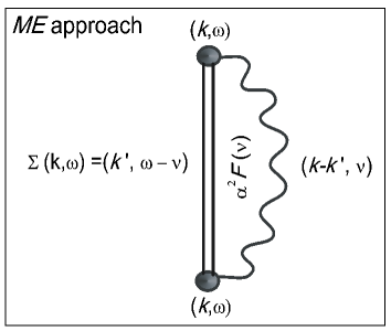
Figure SIII-1: Feynman diagram for the ME approach. The wavy line represents the phonon Green’s function $D$, the double solid line is the renormalized electron Green’s function $G$, and the shaded circles represent the small electron-phonon vertex corrections which have been neglected in this chapter.

Strictly speaking, the Feynman diagram of Fig. SIII-I represents the lowest perturbation diagram for the self energy of electron quasiparticles $\Sigma(k,i\omega_{n})$, scattered from the state k to k’ through the phonon propagator,

$$\Sigma(k,i\omega_{n})=-\beta^{-1}\sum_{k^{\prime},\nu}\langle k|\nabla_{\alpha}V|k^{\prime}\rangle D_{\alpha,\beta}(k-k^{\prime},i\omega_{\nu})\langle k^{\prime}|\nabla_{\beta}V|k\rangle G(k^{\prime},i\omega_{n}-i\omega_{\nu})\,.$$

Here, we have assumed that the electron correlations are responsible of the formation of quasiparticles which are well defined near the Fermi level. In addition, the so called vertex corrections can be a priori neglected because these can be shown to be reduced by the ratio between the phonon frequency ($0-100\leavevmode\nobreak\ meV$) and $\varepsilon_{F}$ ($\sim 1-10\leavevmode\nobreak\ eV$). Thus, the presence of strong electron correlations mediated by the electron-phonon interaction is avoided, and the multi-phonon excitations are reduced to the single-loop approximation or ME approach. The advantage of this formulation is that the electron self energy can be defined in terms of an experimental spectral density which allow estimate the interaction between the electrons and the lattice vibrations for each one of the materials. In this sense, is useful define the E-Ph spectral density as

$$\alpha^{2}F(k,k^{\prime},\nu)\equiv N(0)\langle k|\nabla_{\alpha}V|k^{\prime}\rangle B_{\alpha,\beta}(k-k^{\prime},\nu)\langle k^{\prime}|\nabla_{\beta}V|k\rangle\,,$$

where $N(0)=\sum_{k}\delta(\varepsilon_{k})$ represents the single-spin electronic density of states at the Fermi surface.

Is to be mentioned, that some of the photoemission experiments require consider the complexities of the $d-$band electron structure, and phonons from the “angular” and “energy” components of the phase space ($k$). Then, the $k$-space can be represented in terms of its harmonic components $(J,\varepsilon)$ [32], and the electron self energy can be defined in terms of this set as,

$$\Sigma_{J}(k,i\omega_{n})=T\sum_{J^{\prime},\nu}\int_{0}^{\infty}d\varepsilon^{\prime} \frac{N(\varepsilon^{\prime})}{N(0)}\int_{0}^{\infty}d\nu\alpha^{2}\emph{F}(J,J^{\prime},\varepsilon,\varepsilon^{\prime},\nu)$$

$$\left(\frac{2\nu}{\omega_{\nu}^{2}+\nu^{2}}\right)G_{J^{\prime}}(\varepsilon^{\prime},i\omega_{n}-i\omega_{\nu})\,.$$

The electron-phonon spectral density $\alpha^{2}\emph{F}(J,J^{\prime},\varepsilon,\varepsilon^{\prime},\nu)$ represents a measure of the effectiveness of the phonons of frequency $\nu$ in the scattering of electrons from $k(J,\varepsilon)$ to $k^{\prime}(J^{\prime},\varepsilon^{\prime})$. Here, only the harmonic approximation to the phonon propagator $D(k-k^{\prime},\nu)=2\nu/(\omega_{\nu}^{2}+\nu^{2})$ has been considered. Nevertheless, the above equation for the electron self energy is still cumbersome, and requires an accurate determination of the electron-phonon spectral density from theoretical ab-initio calculations. Then, to avoid this tricky procedure our position is invoke the ME approach.

In order, the ME approach consists in simplify $\Sigma_{J}(k,i\omega_{n})$ by assuming that, it is possible to neglect the dependence on the energy surfaces ($\varepsilon,\varepsilon^{\prime}$) of the $N(\varepsilon^{\prime})\alpha^{2}F(J,J^{\prime},\varepsilon,\varepsilon^{\prime},\nu)$ function. This allow omit the processes violating the Born-Oppenheimer adiabatic theorem contained within the high order graphs. Formally, this means that the spectral function $\alpha^{2}F(JJ^{\prime},\nu)$ is to be diagonal where its representation for the normal state will continue to hold in the superconducting state for the isotropic Cooper pairing or $s$-wave gap. However, other pairing schemes which break rotation symmetry are, in principle, possible [33, 34].

Thus, taking advantage that the ARPES measurements at the nodal direction are not influenced by the anisotropy of the superconducting gap, we will refer to a (non-directional) isotropic quasiparticle spectral density, defined as the double average over the Fermi surface of the electron-phonon spectral density $\alpha^{2}F(\textbf{k},\textbf{k}^{\prime},\nu)$; i.e.,

$$\alpha^{2}F(\nu)=\frac{1}{N(0)}\sum_{\textbf{kk'},j}|g_{\textbf{kk'}}^{j}|^{2}\delta(\nu-\nu_{\textbf{k}-\textbf{k'}}^{j})\delta(\varepsilon_{k})\delta(\varepsilon_{k^{\prime}})\,,$$

where, $g_{\textbf{k}\textbf{k}^{\prime}}^{j}=[\hbar/2M\nu^{j}_{\textbf{k}^{\prime}\textbf{k}}]^{1/2}\langle\textbf{k}|\hat{\epsilon}^{\;j}_{\textbf{k}^{\prime}\textbf{k}}\cdot\nabla V|\textbf{k}^{\prime}\rangle$ defines the matrix elements of the E-Ph interaction for electron scattering from k to k’ with a phonon of frequency $\nu_{\textbf{k}-\textbf{k'}}^{j}$ ($j$ is a branch index). $V$ stands for the crystal potential, $\hat{\epsilon}^{\;j}_{\textbf{k}^{\prime}\textbf{k}}$ is the polarization vector, and $\delta(x)$ denotes the Dirac’s delta function evaluated at $x^{\prime}=0$.

Notice that, $|g_{\textbf{k}\textbf{k}^{\prime}}^{j}|^{2}$ is inversely proportional to the number of charge carriers contributed by each atom of the crystal to the bosonic coupling mode. Therefore, an increase in the doping level, which causes an increment in the hole concentration of the $CuO_{2}$ plane must be reflected in the coupling parameters as we will show in chapter 8. Moreover, recalling the outstanding feature of the theory of metals, that $|g_{\textbf{k}\textbf{k}^{\prime}}^{j}|^{2}$ vanishes linearly with $|\textbf{k}-\textbf{k}^{\prime}|$ when $|\textbf{k}-\textbf{k}^{\prime}|\ll{k}_{F}$ [35], one would expect a linear disappearance of the coupling effect that gives rise to the nodal kink in the vicinity of the Fermi surface. Thus, inspired by recent results on the “universality” of the nodal Fermi velocity $v_{F<}$ (at low energies) in the HTSC, a prominent role of this quantity is also expected.

Finally, in photoelectron scattering experiments the relevant dynamical information is contained in the analytic continuation $G(k,\omega+i0^{+})$ to points just above the real frequency axis, known as the “retarded” Green’s function [30]. One is therefore led to continue the electronic self-energy $\Sigma(k,i\omega_{n})$ analytically by $\Sigma(k,\omega+i0^{+})\equiv\Sigma_{1}(k,\omega)+i\Sigma_{2}(k,\omega)$, where the bare electron band energy is determined by the poles of the Green’s function $G(k,\omega+i0^{+})$ or the zeros of $G^{-1}(k,\omega+i0^{+})$.

Assuming that a pole occurs near $\omega=0$, one gets

$$G^{-1}(k,\omega+i0^{+}) =\omega-\varepsilon_{k}-\Sigma_{1}(k,\omega)-i\Sigma_{2}(k,\omega)$$

$$\simeq\omega\left(1-\left.\frac{\partial\Sigma_{1}(k,\omega)}{\partial\omega}\right|_{\omega=0}\right)-\left[\varepsilon_{k}+\Sigma_{1}(k,0)\right]-i\Sigma_{2}(k,\omega)\,.$$

Then, the pole of $G$ occurs at a frequency $\omega_{0}$ given by $\omega_{0}=E_{k}-i/2\tau_{k}$, with the quasiparticle scattering time defined by $\tau_{k}^{-1}=-2\left(1-\partial_{\omega}\Sigma_{1}\right)^{-1}\Sigma_{2}(k,E_{k})$, and the electron dressed band energy $E_{k}$ by

$$E_{k}=(1-\partial_{\omega}\Sigma_{1})^{-1}\left[\varepsilon_{k}+\Sigma_{1}(k,0)\right]\,.$$

Part IV Addenda

Glossary

In order to provide an easiest reading of this book, below we introduce a list of the most used abbreviations in text. Greek symbols are either incorporated by their phonetic translation into Latin.

• A

  A. Magnetic vector potential.

  AC. Alternate Cycle.

  ARPES. Angle resolved photoemission spectroscopies.

• B

  B. Magnetic induction field (Bold-facing means vector).

  $B_{\tt{a}}$. Peak amplitude for the AC excitation $B_{0}$.

  $B_{0}$. Applied magnetic flux density.

  $B_{p}$. Penetration field.

  $B_{ind}$. Self (induced) magnetic flux density.

  Bi2212. $Bi_{2}Sr_{2}CaCu_{2}O_{8+x}$.

  Bi2201. $Bi_{2}Sr_{1.65}La_{0.35}CuO_{6+x}$.

  Bi-2221. $(Bi,Pb)_{2}Sr_{2}Ca_{2}Cu_{3}O_{x}$

  BM. Brandt-Mikitik

• C

  $\chi$. Bandwidth of the critical state material law incorporated by the SDCST, i.e., $J_{c\parallel}/J_{c\perp}$.

  CS. Critical state.

• D

  $\Delta$. Variation (increment) of …

  $\Delta_{0}$. The zero temperature superconducting gap (Only used within the third part of this dissertation).

  $\Delta_{\textbf{r}}$. Material law for the critical state problems.

  DC. Direct current.

  DCSM. Double critical state model.

• E

  E. Induced transient electric field (In bold means vector).

  $E_{c}$. Critical electrical field.

  $E_{F}$. Electron energy at the Fermi level.

  $E_{k}$. Electron dressed band energy.

  $\varepsilon_{k}$. Electron bare band energy.

  E-Ph. Electron-Phonon.

  EDC. Energy Distribution Curves.

  EDCSM. Elliptical double critical state models.

  Eq(s). Equation(s).

• F

  ${\cal F}$. Minimization functional or so-called Objective function.

  Fig(s). Figure(s)

• H

  H. Magnetic field (In bold means vector).

  HTSC. High-temperature superconducting copper oxides.

• I

  $I_{\tt{a}}$. Peak amplitude for the AC excitation $I_{tr}$.

  $I_{c}$. Critical current.

  $I_{tr}$. Transport current.

  $I_{\parallel}$. Parallel current.

  $I_{\perp}$. Perpendicular current.

  ICSM. Isotropic critical state model.

  INS. Inelastic Neutron Scattering.

• J

  J. Electrical current density (In bold means vector).

  $J_{c}$. Critical current density.

  $J_{c\parallel}$. Parallel component of J.

  $J_{c\perp}$. Perpendicular component of J.

• K

  $k_{B}$. Boltzmann’s constant.

  $k_{F}$. Electrom momentum at the Fermi level

• L

  ${\cal L}$. Lagrange density.

  $L$. Hysteretic AC loss.

  $\lambda$. Electron-phonon coupling parameter.

  $\lambda^{*}$. Mass-enhancement parameter.

  LANCELOT. A FORTRAN package for large-scale nonlinear optimization.

  LEED. Low electronic energy diffraction.

  LSCO. $La_{2-x}Sr_{x}CuO_{4}$.

• M

  $\mu^{*}$. Coulomb psudopotential.

  $\mu_{0}$. Permeability of the free space.

  $\mu_{r}$. Relative permeability associated to a ferromagnetic. material.

  M. Magnetization (In bold means vector).

  $M_{ij}$. Mutual/Self inductance matrix.

  MDC. Momentum distribution-curves.

  ME. Migdal-Eliashberg.

  MRI. Magnetic resonance imaging.

• N

  n. Smoothing index.

• O

  $\omega$. Electromagnetic oscillating frequency.

  $\Omega$. Superconducting volume.

  OPD. Optimally doped.

  OVD. Over doped.

• P

  $\Phi$. SC volume.

  $\varPhi$. Electric scalar potential.

  p. Lagrange multiplier.

  Pag(s). Page(s).

• R

  $R$. Radius of the cylinder.

• S

  S. Poynting’s vector.

  SC. Superconductor.

  SDCST. Smooth double critical state theory.

  SIF. Standard Input Format.

  STM. Scanning tunneling microscopy.

• T

  $T_{c}$. Superconducting critical temperature.

  TCSM. T critical state model.

• U

  UD. Under doped.

• X

  XRS. X-ray scattering.

• Y

  Y123. $YBa_{2}Cu_{3}O_{6+x}$.

Publications

Some of the results presented in this dissertation have been published in the following scientific communications:

1. H. S. Ruiz, A. Badía-Majós, Yu. A. Genenko, S.V. Yampolskii and H. Rauh.
   Applied Physics Letters. February 24, 2012. AIP ID: 102211APL
   Superconducting wires under simultaneous oscillating sources: Magnetic response, dissipation of energy and low pass filtering.

2. H. S. Ruiz and A. Badía-Majós.
   Current Applied Physics 12, 550 (2012).
   Strength of the phonon-coupling mode in $La_{2-x}Sr_{x}CuO_{4}$,
   $Bi_{2}Sr_{2}CaCu_{2}O_{8+x}$ and $YBa_{2}Cu_{3}O_{6+x}$ composites along the nodal direction.

3. H. S. Ruiz, A. Badía-Majós and C. López.
   Superconductor Science and Technology 24, 115005 (2011).
   Material laws and related uncommon phenomena in the electromagnetic response of type – II superconductors in longitudinal geometry.

4. H. S. Ruiz, C. López and A. Badía-Majós.
   Physical Review B 83, 014506 (2011).*
   Inversion mechanism for the transport current in type – II superconductors.
   * Selected for the Virtual Journal of Applications of Superconductivity, Vol 29, Issue 9 (May 1st, 2011), Properties Important for Applications.

5. H. S. Ruiz and A. Badía-Majós.
   Journal of Superconductivity and Novel Magnetism 24, 1273 (2011).
   Relevance of the Phonon-Coupling Mode on the Superconducting Pairing Interaction of $La_{2-x}Sr_{x}CuO_{4}$.

6. H. S. Ruiz and A. Badía-Majós and.
   Superconductor Science and Technology 23, 105007 (2010).
   Smooth double critical state theory for type – II superconductors.

7. A. Badía-Majós, C. López and H. S. Ruiz.
   Physical Review B 80, 144509 (2009).*
   General critical states in type – II superconductors.
   * Selected for the Virtual Journal of Applications of Superconductivity, Vol 17, Issue 8 (October 15th, 2009), Properties Important for Applications.

8. H. S. Ruiz and A. Badía-Majós.
   Physical Review B 79, 054528 (2009).*
   Nature of the nodal kink in angle-resolved spectra of cuprate superconductors.
   * Selected for the Virtual Journal of Applications of Superconductivity, Vol 16, Issue 5 (March 1st, 2009), Materials Important for Applications.

Acknowledgments

I am especially thankful for the great confidence and support provided by my advisor Dr. Antonio Badía-Majós.

I would like also to express my gratitude to Dr. Luis Alberto Angurel and Dr. Rafael Navarro for their undeniable support along my different stages at University of Zaragoza. I also thank to Dr. Yuri Genenko, Dr. Sergey Yampolskii, and Dr. Hermann Rauh, for the interesting discussions we held in Darmstadt University of Technology, as well as for their generous hospitality.

Thanks to the Spanish National Research Council (CSIC), the Institute of Materials Science of Arágon (ICMA), and the Department of Condensed Matter Physics of the University of Zaragoza by their academic and economical support.

Finally but not less important, a special thankful to my girlfriend Edna Corredor, who shares the same passion for physics than me. Without her inexhaustible patience and support, as well as that from my family, this would have not been possible.

It is to be mentioned that, funding of the research within this dissertation has been sponsored by the JAE program of the Spanish National Research Council (CSIC). Also, the attendance to events and dissemination of results was supported by the Spanish CICyT and FEDER program (projects No. MAT2008-05983-C03-01, MTM2006-10531, and MAT2005-06279-C03-01), the DGA project PI049/08, and DGA grant T12/2011.

I authorize to the University of Zaragoza for the distribution and reproduction of this thesis in the digital repositories of ZAGUAN and TESEO, as well as any other one by direct consent of the University of Zaragoza, the Institute of Materials Science of Arágon (ICMA), or the Spanish National Research Council (CSIC).

© Harold Steven Ruiz Rondan

References

- [1]
- [2] C. P. Bean, Rev. Mod. Phys. 36, 31 (1964).
- [3] J. R. Clem, Phys. Rev. B 26, 2463 (1982); J. R. Clem and A. Pérez-González, Phys. Rev. B 30, 5041 (1984); A. Pérez-González and J. R. Clem, Phys. Rev. B 31, 7048 (1985); J. Appl. Phys. 58, 4326 (1985); Phys. Rev. B 32, 2909 (1985); J. R. Clem and A. Pérez-González, Phys. Rev. B 33, 1601 (1986); A. Pérez-González and J. R. Clem, Phys. Rev. B 43, 7792 (1991); F. Pérez-Rodríguez, A. Pérez-González, J. R. Clem, G. Gandolfini, M. A. R. LeBlanc, Phys. Rev. B 56, 3473 (1997).
- [4] A. Badía-Majós, C. López, and H. S. Ruiz, Phys. Rev. B 80, 144509 (2009); and references therein.

References

- [1]
- [2] A. Badía-Majós, C. López, and H. S. Ruiz, Phys. Rev. B 80, 144509 (2009).
- [3] H. S. Ruiz, and A. Badía-Majós, Supercond. Sci. Technol. 23, 105007 (2010).
- [4] J. R. Clem, Phys. Rev. B 26, 2463 (1982); J. R. Clem and A. Pérez-González, Phys. Rev. B 30, 5041 (1984); A. Pérez-González and J. R. Clem, Phys. Rev. B 31, 7048 (1985); J. Appl. Phys. 58, 4326 (1985); Phys. Rev. B 32, 2909 (1985); J. R. Clem and A. Pérez-González, Phys. Rev. B 33, 1601 (1986); A. Pérez-González and J. R. Clem, Phys. Rev. B 43, 7792 (1991); F. Pérez-Rodríguez, A. Pérez-González, J. R. Clem, G. Gandolfini, M. A. R. LeBlanc, Phys. Rev. B 56, 3473 (1997).
- [5] I. F. Voloshin, A. V. Kalinov, S. E. Savel’ev, L. M. Fisher, V. A. Yampol’skiĭ and F. Pérez-Rodríguez, Zh. Ėksp. Teor. Fiz. 111, 1071 (1997) [JETP 84, 592 (1997)].
- [6] L. M. Fisher, K. V. Il’enko, A. V. Kalinov, M. A. R. LeBlanc, F. Pérez-Rodríguez, S. E. Savel’ev, I. F. Voloshin, and V. A. Yampol’skiĭ, Phys. Rev. B 61, 15382 (2000).
- [7] I. F. Voloshin, A. V. Kalinov, L. M. Fisher, S. A. Derevyanko, and V. A. Yampol’skiĭ, Zh. Ėksp. Teor. Fiz. 73 324 (2001) [JETP Letters 73, 285 (2001)].
- [8] L. M. Fisher, A. V. Kalinov, S. E. Savel’ev, I. F. Voloshin and V. A. Yampol’skiĭ, Solid State Commun. 103, 313 (1997).
- [9] I. F. Voloshin, L. M. Fisher, and V. A. Yampol’skiĭ, Low Temp. Phys. 36, 39 (2010).
- [10] L. M. Fisher, A. V. Kalinov, M. A. R. LeBlanc, F. Pérez-Rodríguez, S. E. Savel’ev, I. F. Voloshin, and V. A. Yampol’skiĭ, Physica B 284, 863 (2000).
- [11] I.V. Baltaga, N.M. Makarov, V. A. Yampol’skiĭ, L. M. Fisher, N. V. Il’in, and I. F. Voloshin, Phys. Lett. A 148, 213 (1990); G. P. Gordeev, L. A. Akselrod, S. L. Ginzburg, V. N. Zabenkin, I. M. Lazebnik, Phys. Rev. B 55, 9025 (1997); S. L. Ginzburg, O. V. Gerashenko, A. I. Sibilev, Supercond. Sci. Technol. 10, 395 (1997); S. L. Ginzburg, V. P. Khavronin, and I. D. Luzyanin, Supercond. Sci. Technol. 11, 255 (1988); J. L.Giordano, J. Luzuriaga, A. Badía, G. Nieva, and I. Ruiz-Tagle, Supercond. Sci. Technol. 19, 385 (2006).
- [12] The two velocity hydrodynamic model assumes the existence of two vortex subsystems, A and B, with the same density of vortices, , which are characterized by the average tilt angles, and , with respect to the field orientation. The characteristics flow velocities, and , are expressed in terms of the average hydrodynamic velocity, , and the relative velocity , such that the motion of the vortex system changes and , by satisfying the continuity equations (i) , and (ii) The vortex mean free path represents the relation of the intervortex distance to the averaged probability of the flux line cutting at the vortices intersection. Thus, for determined conditions of the force balance for each one of the sublattices A and B, the above set of equations allows (qualitatively) predicting the magnetization collapse effect by means the arbitrary parameters and , as well as by the knowledge of (more details in Refs. [5, 6, 7, 8, 10, 9]).
- [13] E. H. Brandt and G. P. Mikitik, Phys. Rev. B 76, 064526 (2007).
- [14] The helical model is based upon the use of the torque balance equation for neighboring fluxoids subjected to a torsionally rotating angle , in an analogous manner to the usual force balance equation, such that the translational fluxoid motion obeys the set of equations (i) , and (ii) where is an scalar function, which together with are fitting parameters which are not obtained directly as functions of (more details in Refs. [21, 22, 23]).
- [15] J. R. Clem, M. Weigand, J. H. Durrell and A. M. Campbell, Supercond. Sci. Technol. 24, 062002 (2011).
- [16] A. M. Campbell, Supercond. Sci. Technol. 24, 091001 (2011).
- [17] V. R. Karasik and v. G. Vereshchagin, Zh. Eksp. Teor. Fiz. 59, 36 (1970) [Sov. Phys.-JETP 32, 20 (1971)].
- [18] A. Badía and C. López, Phys. Rev. Lett. 87, 127004 (2001).
- [19] E. H. Brandt, J. R. Clem, and D. G. Walmsley, J. Low Temp. Phys. 37, 43 (1979).
- [20] J. R. Clem and S. Yeh, J. Low Temp. Phys. 39, 173 (1980). J. R. Clem, J. Low Temp. Phys. 38, 353 (1980), and references quoted therein.
- [21] T. Matsushita and F. Irie, J. Phys. Soc. Japan 54, 1066 (1985).
- [22] T. Matsushita, A. Shimogawa and M. Asano, Physica C 298, 115 (1998).
- [23] T. Matsushita, Japanese. Journ. Appl. Phys. 51, 010111 (2012).
- [24] K. Watanabe, H. Yamane, N. Kobayashi, T. Hirai and Y. Muto, Studies of High-Temperature Superconductors vol 8 (New York: Nova Science, 1992) pag. 107.
- [25] A. Sánchez, C. Navau, N. Del-Valle, D. X. Chen and J. R. Clem, Appl. Phys. Lett. 96, 072510 (2010).
- [26] M. G. Blamire, C. H. Marrows, N. A. Stelmashenko and J. E. Evetts, Phys. Rev. B 67, 014508 (2003).
- [27] M. G. Blamire and J. E. Evetts, Phys. Rev. B 33, 5131 (1986).
- [28] R. Boyer, G. Fillion and M. A. R. LeBlanc, J. Appl. Phys. 51, 1692 (1980).
- [29] R. Gauthier, M. A. R. LeBlanc and B. C. Belanger, Proceedings of Low Temperature Physics-LT13 vol 3 (New York: Plenum, 1974) pag. 241.
- [30] M. Sugahara, Japan. J. Appl. Phys. 9, 625 (1970).
- [31] H. F. Taylor, Appl. Phys. Lett. 11, 169 (1967).
- [32] S. T. Sekula, R. W. Boom and C. J. Bergeron, Appl. Phys. Lett. 2, 102 (1963).
- [33] H. S. Ruiz, C. López and A. Badía-Majós, Phys. Rev. B 83, 014506 (2011).
- [34] H. S. Ruiz, A. Badía-Majós, and C. López, Supercond. Sci. Technol. 24, 115005 (2011).
- [35] M. A. R. LeBlanc and S. Çelebi, Supercond. Sci. Technol. 16, 329 (2003).
- [36] S. Çelebi and M. A. R. LeBlanc, Studies of High-Temperature Superconductors vol 42 (New York: Nova Science, 2002) pag. 169.
- [37] M. A. R. LeBlanc, S. Çelebi, S. X. Wang and V. Plechácêk, Phys. Rev. Lett. 71, 3367 (1993).
- [38] M. A. R. LeBlanc, D. LeBlanc, A. Golebiowski and G. Fillion, Phys. Rev. Lett. 66, 3309 (1991).
- [39] I. F. Voloshin, N. V. II’in, N. M. Makarov, L. M. Fisher and V. A. Yampol’skiĭ, JETP Lett. 53, 116 (1991).
- [40] J. R. Cave and J. E. Evetts, Phil. Mag. B 37, 111 (1978).
- [41] D. G. Walmsley and W. E. Timms, J. Phys. F 7, 2373 (1977).
- [42] T. Esaki and F. Irie, J. Phys. Soc. Japan 40, 382 (1976).
- [43] D. G. Walmsley, J. Phys. F 2, 510 (1972).
- [44] H. London and D. G. Walmsley, Proc. 11th Int. Conf. Low Temp. Phys. (St. Andrews, 1968) pag. 879.
- [45] M. A. R. LeBlanc, Phys. Rev. 143, 220 (1966).
- [46] J. R. Clem, Phys. Rev. B 83, 214511 (2011).
- [47] Y. Nakayama, Proceedings of the 4th International Cryogenic Engineering Conference (Guildford: IPC Science and Technology Press, 1972) pag. 133.
- [48] C. J. Bergeron, Appl. Phys. Lett. 3, 63 (1963).
- [49] C. P. Bean, Rev. Mod. Phys. 36, 31 (1964); C. P. Bean, J. Appl. Phys. 41, 2482 (1970).
- [50] H. S. Ruiz, A. Badía-Majós, Yu. A. Genenko, S.V. Yampolskii and H. Rauh. arXiv:1108.0659 [cond-mat.supr-con]. To appear in Appl. Phys. Lett. (March-2012).
- [51] H. London, Phys. Lett. 6, 162 (1963).
- [52] R. Hancox, Proc. IEE 113, 1221 (1966).
- [53] W.J. Carr, Jr., M.S. Walker, and J.H. Murphy, J. Appl. Phys. 46, 4048 (1975).
- [54] V.B. Zenkevitch, V.V. Zeltov, A.S. Romanyuk, Cryogenics 18, 93 (1978), Sov. Phys. Dokl. 25, 210 (1980); V.B. Zenkevitch, A.S. Romanyuk, V.V. Zeltov, Cryogenics 20, 703 (1980).
- [55] J.V. Minervini, IEEE Trans. Mag., 25, 2113 (1989).
- [56] W.J. Carr, AC loss and macroscopic theory of superconductors 2nd Ed. (Taylor & Francis, NY, 2001).
- [57] A.V. Gurevich, R.G. Mints, A.L. Rakhmanov, Physics of composite superconductors, (Nauka Publishers, 1987 in Russian) [Engl. translation: Begell House, NY, 1997].
- [58] G. W. Swan, J. Math. Phys. 9, 1308 (1968).
- [59] M. R. Halse, J. Phys. D 3, 717 (1970).
- [60] W. T. Norris, J. Phys. D 3, 489 (1970).
- [61] E. H. Brandt and M. Indenbom, Phys. Rev. B 48, 12893 (1993); E. H. Brandt, M. V. Indenbom, and A. Forkl, Europhys. Lett. 22, 735 (1993) .
- [62] E. Zeldov, J. R. Clem, M. McElfresh, and M. Darwin, Phys. Rev. B 49, 9802 (1994).
- [63] Y. Mawatari, Phys. Rev. B 83, 134512 (2011).
- [64] M. Ashkin, J. Appl. Phys. 50, 7060 (1979); M. Ashkin, G.R. Wagner, J. Appl. Phys. 60, 2477 (1986).
- [65] M. Ashkin, G. R. Wagner, J. Appl. Phys. 60, 2477 (1986).
- [66] C. Y. Pang, A. M. Campbell, and P. G. McLauren, IEEE Trans. Magn. 17, 134 (1981).
- [67] K.L. Telschow and L.S. Koo, Phys. Rev. B 50, 6932 (1994).
- [68] Y.E. Kuzovlev, JETP Lett. 61, 1000 (1995).
- [69] K.V. Bhagwat, D. Karmakar, Pramana 57, 763 (2001); D. Karmakar, K.V. Bhagwat, Physica C 398, 20 (2003).
- [70] R. Navarro and L. J. Campbell, Phys. Rev. B 44, 10146 (1991).
- [71] F. Gömöry, R. Tebano, A. Sanchez, E. Pardo, C. Navau, I. Husek, F. Strycek, and P. Kovac, Supercond. Sci. Technol. 15, 1311 (2002).
- [72] B. ten Haken, J.J. Rabbers, H.H.J. ten Kate, Physica C 377, 156 (2002).
- [73] N. Amemiya and Y. Ohta, Physica C 357-360, 1134 (2001).
- [74] N. Nibbio, S. Stavrev, IEEE Trans. Appl. Supercond. 11, 2627 (2001).
- [75] S. Stavrev, B. Dutoit, and N. Nibbio, IEEE Trans. Appl. Supercond. 12, 1857 (2002).
- [76] Z. Hong, L. Ye, M. Majoros, A.M. Campbell, J. Supercond. Nov. Magn. 21, 205 (2008).
- [77] L. Prigozhin, Physica D 197, 197 (2004).
- [78] J. W. Barrett and L. Prigozhin, Math. Models Meth. Appl. Sci. 20, 1 (2010).
- [79] A. M. Campbell, Supercond. Sci. Technol. 20, 292 (2007); A. M. Wolsky and A. M. Campbell, Supercond. Sci. Technol. 21, 1 (2008).
- [80] S. Farinon, P. Fabbricatore, and F. Gömöry, Supercond. Sci. Technol. 23, 1 (2010).
- [81] E. H. Brandt, Phys. Rev. B 54, 4246 (1996).
- [82] D. Larbalestier, A. Gurevich, D. M. Feldmann and A. Polyanskii, Nature. 414, 368 (2001).
- [83] M. P. Oomen, J. Rieger, V. Hussennether and M. Leghissa, Supercond. Sci. Technol. 17, S394 (2004); M. P. Oomen, R. Nanke and M. Leghissa, Supercond. Sci. Technol. 16, 339 (2003).
- [84] J. R. Hull, Rep. Prog. Phys. 66, 1865 (2003).
- [85] N. B. Paul, M. D. Sumption and G. L. Rhoads, Cryogenics 45, 670 (2005).
- [86] M.I. Yunus, Y. Iwasa, J.E.C. Williams, Cryogenics 35, 93 (1995).
- [87] K. Takeuchi, Y.K. Kang, H. Hashizume, and Y. Iwasa, Cryogenics 38, 367 (1998).
- [88] W. J. Carr, IEEE Trans. Magn. 15, 240 (1979).
- [89] N. Schönborg, J. Appl. Phys. 90, 2930 (2001).
- [90] N. Amemiya, K. Miyamoto, S. Murasawa, H. Mukai and K. Ohmatsu, Physica C 310, 30 (1998).
- [91] T. Yazawa, J. J. Rabbers, B. ten Haken, H. H. J. ten Kate and Y. Yamada, Physica C 310, 36 (1998).
- [92] T. Yazawa, J. J. Rabbers, O. A. Shevchenko, B. ten Haken and H. H. J. ten Kate, IEEE Trans. Appl. Supercond. 9, 797 (1999).
- [93] S. Zannella, L. Montelatici, G. Grenci, M. Pojer, L. Jansak, M. Majoros, G. Coletta, R. Mele, R. Tebano and F. Zanovello, IEEE Trans. Appl. Supercond. 11, 2441 (2001).
- [94] R. Tebano, R. Mele, V. Boffa, F. Gömöry, F. Strýček and E. Seiler, Int. J. Mod. Phys. B 17 528 (2003).
- [95] H. Tonsho, S. Fukui, T. Sato, M. Yamaguchi, S. Torii, T. Takao and K. Ueda, IEEE Trans. Appl. Supercond. 13 2368 (2003).
- [96] J. Ogawa, M. Shiokawa, M. Ciszek and O. Tsukamoto, IEEE Trans. Appl. Supercond. 13 1735 (2003).
- [97] N. Enomoto and N. Amemiya, Physica C 412-414, 1050 (2004).
- [98] S. Stavrev, F. Grilli, B. Dutoit and S. P. Ashworth, Supercond. Sci. Technol. 18, 1300 (2005).
- [99] D. N. Nguyen, S. V. Pamidi, D. C. Knoll, G. Zhang, and J. Schwartz, Journ. Appl. Phys. 98, 073902 (2005).
- [100] D. N. Nguyen, P.V.P.S.S. Sastry, G. M. Zhang, D. C. Knoll and J. Schwartz, IEEE Trans. Appl. Supercond. 15, 2831 (2005).
- [101] M. Vojenčiak, J. Šouc, J. M. Ceballos, F. Gömöry, B. Klinčok, E. pardo, and F. Grilli, Supercond. Sci. Technol. 19, 397 (2006).
- [102] E. Pardo, F. Gömöry, J. Šouc and J. M. Ceballos, Supercond. Sci. Technol. 20, 351 (2007).
- [103] E. Pardo, A. Sanchez, D.-X Chen and C. Navau, Phys. Rev. B 71, 134517 (2005); E. Pardo, D.-X. Chen, A. Sanchez, and C. Navau, Supercond. Sci. Technol. 17, 83 (2004); E. Pardo, A. Sanchez and C. Navau, Phys. Rev. B 67, 104517 (2003).
- [104] W. Pi, Y.-S. Wang, J. Dong and L. Chen, Chin. Phys. Lett. 27, 037401 (2010).
- [105] K. P. Thakur. A. Raj, E. H. Brandt, J. Kvitkovic and P.V.P.S.S. Sastry, Supercond. Sci. Technol. 24, 045006 (2011).
- [106] K. P. Thakur. A. Raj, E. H. Brandt, and S. V. Pamidi, Supercond. Sci. Technol. 24, 0650624 (2011).
- [107] Y. Iwasa, Case Studies in Superconducting Magnets: Design and Operational Issues (Springer Science+Business Media, NY, 2009).
- [108] P. Wanderer, Exotic Magnets for Accelerators ( 19th International Conference on Magnet Technology), in Superconducting Magnet Division Brookhaven National Laboratory, http://www.bnl.gov/magnets/magnet_files/Publications/... ...BNL-75350-2006-CP.pdf
- [109] V. S. Kashikhin, N. Andreev, V. V. Kashikhin, I. Novitski and A. Zlobin, IEEE Trans. Appl. Supercond. 16, 1274 (2006).
- [110] P. He, F. T. Wang, Z. M. Chen, W. G. Chen, Z. Y. Chen, J. W. Zhu, Y. Ren and J. J. Li, IEEE Trans. Appl. Supercond. 20, 2331 (2010).
- [111] J. Ogawa, S. Fukui, T. Oka, T. Sato, H. Kojima, M. Shibayama and M. Egawa, IEEE Trans. Appl. Supercond. 21, 3325 (2011)
- [112] R. Inada, H. Kimura, K. Tateyama, Y. Nakamura, A. Oota and P. Zhang, Physica C Part 2 426-431, 1322 (2005).
- [113] Z. Jiang, N. Amemiya, N. Ayai and K. Hayashi, Supercond. Sci. Technol. 17, 1311 (2004).
- [114] J. J. Rabbers, B. ten Haken and H. H. J. ten Kate, Rev. Sci. Instrum. 72, 2365 (2001); Physica C 310, 101 (1998).
- [115] J. L. de Reuver, G. B. J. Mulder, P. C. Rem and L. J. M. van de Klundert, IEEE Trans. Magn. 21, 173 (1985).
- [116] M. Ramos, J. Schwartz,U. Trociewitz, S. Pamidi and S. Flores, Revista Mexicana de Fisica, 56, 172 (2010).
- [117] S. P. Ashworth and M. Suenaga, Physica C 329, 149 (2000).
- [118] N. Magnusson, S. Hörnfeldt, J. J. Rabbers, B. ten Haken and H. H. J. ten Kate, Supercond. Sci. Technol. 13, 291 (2000).
- [119] V. B. Zenkevitch, V. V. Zheltov, and A. S. Romanyuk, Hysteretic losses in windings made up conductores comprising round superconducting filaments (Institute of high temperatures of the USSR, Academy of Sciences, Moscow, 1983). See also Ref. [57], pag. 88.
- [120] T. Hamajima, T. Yagai, and M. Tsuda, IEEE Trans. Appl. Supercond., 16, 1586 (2006).
- [121] T. Hamajima, M. Tsuda, T. Yagai, S. Monma, H. Satoh, and K. Shimoyama, IEEE Trans. Applied Superconductivity, 17, 1692 (2007).
- [122] T. Hamajima, M. Tsuda, T. Yagai, A. Nuri Ozcivan, K. Shimoyama, K. Aoyagi, and S. Soeda, Journal of Physics: Conference Series, 97, 012253 (2008).
- [123] M. J. Gouge, D. T. Lindsay, and J. A. Demko, IEEE Trans. Appl. Supercond. 15, 1827 (2005).
- [124] S Takács, Supercond. Sci. Technol. 20, 1093 (2007).
- [125] Y. Mawatari and K. Kajikawa, Applied Physics Letters, 90, 022506 (2007).

References

- [1]
- [2] J. Bardeen, L. N. Cooper y J. R. Schrieffer, Phys. Rev. 106, 162 (1957); Phys Rev. 108 1175 (1957).
- [3] H. S. Ruiz and A. Badía-Majós, Phys. Rev. B 79, 054528 (2009).
- [4] H. S. Ruiz and A. Badía-Majós, J. Supercond. Nov. Magn. 24, 1273-1280 (2011).