Light scalars in strongly-coupled extra-dimensional theories.

Abstract:

The low–energy dynamics of five–dimensional Yang–Mills theories compactified on $S^{1}$ can be described by a four–dimensional gauge theory coupled to a scalar field in the adjoint representation of the gauge group. Perturbative calculations suggest that the mass of this elementary scalar field is protected against power divergences, and is controlled by the size of the extra dimension $R$. As a first step in the study of this phenomenon beyond perturbation theory, we investigate the phase diagram of a ${\rm SU(}2{\rm)}$ Yang–Mills theory in five dimensions regularized on anisotropic lattices and we determine the ratios of the relevant physical scales. The lattice system shows a dimensionally reduced phase where the four–dimensional correlation length is much larger than the size of the extra dimension, but still smaller than the four–dimensional volume. In this region of the bare parameter space, at energies below $1/R$, the non–perturbative spectrum contains a light scalar state. This state has a mass that is independent of the cut-off, and a small overlap with glueball operators. Our results suggest that light scalar fields can be introduced in a lattice theory using compactified extra dimensions, rather than fine tuning the bare mass parameter.

1 Introduction

Five–dimensional Yang–Mills theories compactified on a circle have a light scalar mode, whose mass renormalization in perturbation theory is protected by the remnant of the higher–dimensional gauge symmetry. This light scalar is the static Kaluza–Klein mode coming from the compactification of the fifth component of the original gauge field, when periodic boundary conditions are imposed [1, 2]. At tree level, this mode is massless. At low energies, the physics of compactified extra–dimensional theories can be described by an effective lagrangian for a four–dimensional gauge theory coupled to an elementary scalar particle in the adjoint representation of the gauge group. This effective description is valid only up to the compactification energy scale $\Lambda_{\rm R}\sim R^{-1}$, where $R$ is the radius of the extra dimension. At the compactification scale, other massive vector modes become relevant for the dynamics, and their coupling to the low–energy spectrum described above can no longer be neglected.
Quantum corrections usually yield divergences in the mass of scalar particles: in a generic renormalizable quantum field theory, the scalar mass receives contributions proportional to the square of the ultra–violet (UV) cut–off. However, the mass of the scalar field coming from the compactification of a higher–dimensional gauge field remains finite, as suggested by one–loop and two–loop calculations  [3, 4, 5, 6, 7, 8].
These perturbative calculations are performed using the explicit four–dimensional effective field theory that describes the five–dimensional system at low energies. The same result has been obtained using the full five–dimensional gauge theory which explicitly includes all the higher energy contributions [9]. Since the extra–dimensional gauge theory is believed to be non–renormalizable, it can only be defined as a regulated theory with an ultra–violet cut–off $\Lambda_{\rm UV}$ always in place. Interestingly the quantum corrections to the scalar mass are independent of $\Lambda_{\rm UV}$:

$$\delta m^{2}\;=\;\frac{9g_{5}^{2}N_{c}}{32\pi^{3}R^{3}}\zeta(3)\;,$$ (1)

where $\zeta$ is the Riemann Zeta–function, $N_{c}$ is the number of colours and $g_{5}^{2}$ is the dimensionful coupling constant of the five–dimensional Yang–Mills theory.
It must be stressed, that Eq. (1) is valid only in the regime where there is a scale separation $\Lambda_{\rm R}\ll\Lambda_{\rm UV}$ between the compactification scale $\Lambda_{\rm R}$ and the cut–off $\Lambda_{\rm UV}$, because in this case the details of the regularization can be neglected. In this energy region, the highly energetic modes at the cut–off scale see the extra dimension as non–compact and therefore do not contribute to the scalar mass corrections, due to the higher–dimensional gauge symmetry.
All the aforementioned results make the compactification mechanism a very interesting and promising scenario to protect the mass of scalar particles from cut–off effects. Moreover, since the early work of Ref. [10], higher–dimensional theories have gained significant phenomenological interest.
In this work, we study this mechanism in the simple case where the extra dimension is compactified on a circle $S^{1}$. In particular, we would like to explore the validity of the perturbative prediction Eq. (1) in the strongly–coupled regime of the theory. While we do not expect the proportionality constant to remain unchanged, we want to check whether the non–perturbative dynamics preserves the independence of the UV cut–off, and the functional dependence on the compactification radius. This is a non-trivial task, since in the non–perturbative regime the states in the spectrum are not the excitations of the elementary fields in the action.
To be able to access the non–perturbative regime, we use Monte Carlo simulations of a lattice gauge theory in five dimensions. We then search for a region in the parameter space of the lattice theory where the hierarchy of scales is such that the low–energy physics is described by a four–dimensional effective theory with a light scalar particle.
In recent years, there have been several numerical studies of the simplest of these extra–dimensional theories on the lattice, namely the ${\rm SU(}2{\rm)}$ pure gauge theory on a five–dimensional torus with anisotropic lattice spacings, $a_{4}$ in the four–dimensional space and $a_{5}$ in the extra fifth dimension [11, 12, 13, 14, 15]. A pioneering study of the same model on isotropic lattices was done in the late seventies [16].
The aim of this work is to explore the parameter space of the lattice model and to define the scales separation by studying the behaviour of observables such as the string tension and the mass of scalar states; this goes in the direction of improving previous recent results [13] and trying to clarify the status of Eq. (1) in the non–perturbative regime. Using numerical simulations in the region of phase space where there is a hierarchy of scales $\Lambda_{\rm R}\ll\Lambda_{\rm UV}$, we are able to study the parametric dependence of the non–perturbative scalar mass on the cut–off $\Lambda_{\rm UV}$ and on the compactification scale $\Lambda_{\rm R}$. However, in order to fully understand the nature of the effective theory and of the scalar particle, more studies are needed that are beyond the scope of this work. In particular, matching simulations between this five–dimensional gauge model and the four–dimensional gauge theory with an adjoint scalar field in the action could be performed, following what was done to test dimensional reduction in lower dimensions [17].
In Sec. 2 we describe the lattice setup used in our simulations of the ${\rm SU(}2{\rm)}$ Yang–Mills theory in five dimensions. In Sec. 3 we explain the separation of scales that we expect to find in the lattice model, and we analyse the perturbative predictions for the behaviour of the desired hierarchy of scales as we scan the bare parameter space. Next, we provide a description of the phase diagram of the model in Sec. 4 and compare our findings with previous studies. Once the phase diagram has been mapped out and the interesting region has been identified, we present the details of our measurements and compare them with the perturbative expectations in Sec. 5. Finally we present a critical discussion of the results and future developments of these ideas.

2 The lattice model

The continuum, five–dimensional pure gauge theory is defined by the Euclidean action

$$\mathcal{S}\;=\;\int\mbox{d}^{4}x\>\int_{0}^{2\pi R}\mbox{d}x_{5}\>\frac{1}{2g_{5}^{2}}{\rm Tr}~{}F_{MN}^{2}\;,$$ (2)

where periodic boundary conditions are imposed along the fifth direction (whose coordinate is $x_{5}$) in order to make it compact. The field–strength tensor is the extra–dimensional generalization of the four–dimensional one

$$F_{MN}\;=\;\partial_{M}A_{N}-\partial_{N}A_{M}+i[A_{M},A_{N}]\quad M,N=1,\dotsc,5\;.$$ (3)

This continuum theory has an infinite four–dimensional volume, but it is defined only on a finite and compact fifth dimension of length $L_{5}=2\pi R$, where $R$ is the compactification radius.
Since this theory is perturbatively non–renormalizable, the ultra–violet cut–off $\Lambda_{\rm UV}$ cannot be removed. For the same reason we consider the action in Eq. (2) only as the simplest non–trivial example of effective theory in five dimensions: an arbitrary number of operators and couplings could be added in principle. Cut–off effects are expected to be irrelevant in the low–energy regime of the theory defined by the action in Eq. (2), i.e. at scales $E\ll\Lambda_{\rm UV}$.
The continuum action is regularized on a five–dimensional lattice, where the finite lattice spacing determines the shortest propagating wavelength. Two independent lattice spacings $a_{4}$ and $a_{5}$ can be defined on the lattice, which correspond respectively to the lattice spacing in the four–dimensional subspace, and in the extra fifth direction; the bigger of the two defines the inverse of the cut–off $\Lambda_{\rm UV}$. The gauge potential $A_{M}(x_{M})$ is replaced on the lattice by gauge link variables $\mathcal{U}_{M}(x)$ joining the site $x$ and the site $x+a\hat{M}$, where $a=a_{4}$ if $M=1,2,3,4$ and $a=a_{5}$ if $M=5$. Periodic boundary conditions for the gauge links are imposed in all five directions.
We choose the anisotropic lattice Wilson action for ${\rm SU(}N_{c}{\rm)}$ gauge theories:

$$\mathcal{S}_{W}\;=\;\beta_{4}\sum_{x;1\leq\mu<\nu\leq 4}\left[1-\frac{1}{N_{c}}{\rm Re}\hskip 1.0pt{\rm Tr}~{}P_{\mu\nu}(x)\right]+\beta_{5}\sum_{x;1\leq\mu\leq 4}\left[1-\frac{1}{N_{c}}{\rm Re}\hskip 1.0pt{\rm Tr}~{}P_{\mu 5}(x)\right]\;,$$ (4)

where $P_{\mu\nu}$ is the four–dimensional plaquette ($\mu$ and $\nu$ run from $1$ to $4$)

$$P_{\mu\nu}(x)\;=\;\mathcal{U}_{\mu}(x)\mathcal{U}_{\nu}(x+\hat{\mu}a_{4})\mathcal{U}_{\mu}^{\dagger}(x+\hat{\nu}a_{4})\mathcal{U}_{\nu}^{\dagger}(x)\;,$$ (5)

and $P_{\mu 5}$ is the plaquette abutting on an extra–dimensional slice

$$P_{\mu 5}(x)\;=\;\mathcal{U}_{\mu}(x)\mathcal{U}_{5}(x+\hat{\mu}a_{4})\mathcal{U}_{\mu}^{\dagger}(x+\hat{5}a_{5})\mathcal{U}_{5}^{\dagger}(x)\;.$$ (6)

The sum is intended to be on all the lattice sites $x$ of the full five dimensional lattice volume.
This lattice setup is the same used in Ref. [11]. However, a different parametrization for the Wilson action can be used [13]:

$$\mathcal{S}_{W}\;=\;\frac{\beta}{\gamma}\sum_{x;1\leq\mu\leq\nu\leq 4}\left[1-\frac{1}{N_{c}}{\rm Re}\hskip 1.0pt{\rm Tr}~{}P_{\mu\nu}(x)\right]+\beta\gamma\sum_{x;1\leq\mu\leq 4}\left[1-\frac{1}{N_{c}}{\rm Re}\hskip 1.0pt{\rm Tr}~{}P_{\mu 5}(x)\right]\;,$$ (7)

where the lattice coupling constant is

$$\beta\;=\;\sqrt{\beta_{4}\beta_{5}}\;,$$ (8)

and the second parameter is the bare anisotropy

$$\gamma\;=\;\sqrt{\frac{\beta_{5}}{\beta_{4}}}\;.$$ (9)

The bare anisotropy is related to the ratio of the lattice spacings $\xi=a_{4}/a_{5}$. At tree level $\gamma=\xi$, but quantum corrections make $\xi$ deviate from this value. The relation between $\xi$ and $\gamma$ for this action has already been studied in bare parameter space and a useful map relating this two quantities can be found in Ref. [11].
In order to obtain Eq. (2) in the classical continuum limit of the action in Eq. (4), we must require the following relations for the lattice parameters (coupling constants) $\beta_{4}$ and $\beta_{5}$:

$$\beta_{4} = \frac{2N_{c}a_{5}}{g_{5}^{2}}$$ (10)

$$\beta_{5} = \frac{2N_{c}a_{4}^{2}}{g_{5}^{2}a_{5}}\;.$$ (11)

Similarly, for the action in Eq. (7) we have

$$\beta\;=\;\frac{2N_{c}}{g_{5}^{2}}a_{4}\;,$$ (12)

and

$$\gamma\;=\;\xi\;=\;\frac{a_{4}}{a_{5}}\;.$$ (13)

In this work we use the Wilson action Eq. (4) with $\beta_{4}$ and $\beta_{5}$ as bare parameters, and therefore our results will be presented as functions of these two quantities. However some of the features of the phase diagram are better explained in terms of $\beta$ and $\gamma$, in particular when comparing our findings to existing results [13].
Finally there are two more parameters in the lattice model that can be adjusted in order to realize the desired separation of scales; they are $N_{4}$, the number of lattice sites in each of the usual four directions, and $N_{5}$, the number of lattice sites in the extra dimension. Together with the corresponding lattice spacings, they determine the physical size of the system: $L_{4}=a_{4}N_{4}$ in four dimensions and $L_{5}=2\pi R=a_{5}N_{5}$ in the fifth dimension.
In the following we restrict ourself to the non–Abelian gauge group ${\rm SU(}2{\rm)}$, thus setting $N_{c}=2$ in the above definitions.

3 Dimensional reduction and scale separations

We have already mentioned that the theory described by the action in Eq. (2) is perturbatively non–renormalizable because the five–dimensional coupling constant $g_{5}^{2}$ has negative mass dimension $M^{-1}$. Moreover, the theory possesses another intrinsic scale when the extra dimension is compactified on the circle: the compactification scale $\Lambda_{\rm R}\sim R^{-1}$. This scale is the analogue of the temperature scale in the formulation of finite–temperature field theories compactified on a circle.
Upon compactification, the gauge fields are decomposed into Fourier modes (called Kaluza–Klein modes in this context, or Matsubara modes in finite–temperature field theories). At the classical level the spectrum of the theory contains massless vectors, coming from the gauge field components in the four–dimensional subspace, and a massless scalar, coming from the gauge component in the extra compact direction. All the higher modes acquire masses proportional to $\Lambda_{\rm R}$. In the quest for an effective description of the low–energy physics of the theory, one can integrate out the states at energies greater than the compactification scale, leaving a four–dimensional gauge field coupled to an adjoint massless scalar. However, this dimensional reduction is a sensible description only if there is a scale separation $\Lambda_{\rm R}\ll\Lambda_{\rm UV}$: the physics of the compactified theory is not affected by the details of the regularization. As discussed below, this condition is only satisfied in a specific region of the lattice bare parameter space.
If we focus on the low–energy $E\ll\Lambda_{\rm R}$ and weakly–coupled regime, we expect a perturbative spectrum, where the elementary scalar particle acquires a mass through radiative corrections, while the gauge vectors remain massless. As we explore more strongly–coupled regimes, the theory develops a non–perturbative mass gap related to confinement. Our aim is to study what happens to the low–lying spectrum of scalar particles in this non–perturbative regime. In particular we would like to understand if there exists a region in the bare parameter space of the five–dimensional theory where the non–perturbative dynamics can be described by a four–dimensional effective gauge theory coupled to a light adjoint scalar, whose mass is decoupled from the cut–off scale as suggested by the one–loop equation Eq. (1). Moreover, it would be interesting to find a region where the scalar mass is of the order of the mass gap in the gauge sector.
A previous study has shown that there is a region of the phase diagram of the lattice model where a scale separation between the static modes of the four–dimensional gauge fields and their higher Kaluza–Klein modes is observed [13, 18], indicating that the theory undergoes dimensional reduction similar to the case of four–dimensional hot gauge theories [19]. However, in that same region, the static mode of the fifth component of the gauge field appears to be completely decoupled, with a mass at the scale of the cut–off, and hence outside the regime of validity of Eq. (1).
Let us summarize now the hierarchy of scales that we would like to find non–perturbatively in the lattice theory described in Sec. 2.

• A separation between the compactification scale and the cut–off

  $$\frac{\Lambda_{\rm UV}}{\Lambda_{\rm R}}\;\gg\;1\;.$$ (14)

• The mass gap identified by the string tension $\sqrt{\sigma}$ in four dimensions must be separated both from the cut–off and from the compactification scales:

  $$\sqrt{\sigma}\;\ll\;\Lambda_{\rm UV}\;{\rm;}\qquad\sqrt{\sigma}\;\ll\;\Lambda_{\rm R}\;.$$ (15)

  In fact, only if the above relations are true, we expect the long distance physics to be independent of the actual regularization of the theory, and not to be sensitive to contributions from higher modes. In other words, since the string tension gives the inverse of the four–dimensional correlation length, when $\sqrt{\sigma}$ is small compared to the cut–off, then the characteristic length of the system is much larger than the lattice spacing, and the details of the discretization of the theory should become insignificant.

• Light scalar states should be at the energy scale defined by the mass gap, and hence their mass, generically referred to as $m_{5}$, should be separated from the cut–off and from the energy scale of the other Kaluza–Klein massive modes:

  $$m_{5}\;\simeq\;\sqrt{\sigma}\;{\rm;}\qquad m_{5}\;\ll\;\Lambda_{\rm UV}\;{\rm;}\qquad m_{5}\;\ll\;\Lambda_{\rm R}\;.$$ (16)

• Finally, we need to check the dependence of the scalar mass from the cut-off and the compactification radius. We would like to find a region in the space of bare parameters, where we have a scaling similar to the one Eq. (1) obtained for an elementary scalar particle in the weakly-coupled regime:

  $$m_{5}^{2}\;\propto\;\frac{g_{5}^{2}}{R^{3}}\;.$$ (17)

In a strongly–coupled theory the different energy scales described above are dynamically generated, and need to be measured by numerical simulations. In the following discussions, we choose to express every scale in units of the four–dimensional string tension $\sqrt{\sigma}$; hence the other three scales in the theory are characterized by three dimensionless ratios. The ultra–violet cut–off $\Lambda_{\rm UV}$, given by the inverse of the largest lattice spacing of the model, is

$$\frac{\Lambda_{\rm UV}}{\sqrt{\sigma}}\;\equiv\;\frac{1}{a_{4}\sqrt{\sigma}}\;,$$ (18)

because we will be dealing with anisotropies $\xi=\frac{a_{4}}{a_{5}}\geq 1$. Similarly, the compactification scale $\Lambda_{\rm R}$ is

$$\frac{\Lambda_{\rm R}}{\sqrt{\sigma}}\;\equiv\;\frac{1}{2\pi R\sqrt{\sigma}}\;=\;\frac{1}{a_{5}N_{5}\sqrt{\sigma}}\;.$$ (19)

Finally, the scalar mass $m_{5}$ can be expressed as the ratio of the scalar mass and the string tension both measured in units of the lattice spacing $a_{4}$ in our simulations:

$$\frac{m_{5}}{\sqrt{\sigma}}\;=\;\frac{a_{4}m_{5}}{a_{4}\sqrt{\sigma}}\;.$$ (20)

In Fig. 1 we summarize pictorially the scale separations in the theory.

Figure 1: The figure shows the desired separation of energy scales. The scales are all expressed in terms of the four–dimensional string tension that characterizes the low–energy physics of the theory. The region of energies where we expect the scalar mass to lie is highlighted by the shaded band.

Let us note that the separation of the UV and the compactification scales can be entirely expressed in terms of bare parameters of the lattice model at tree level:

$$\frac{\Lambda_{\rm UV}}{\Lambda_{\rm R}}\;\equiv\;\frac{a_{5}N_{5}}{a_{4}}\;=\;\frac{N_{5}}{\xi}\;\sim\;\frac{N_{5}}{\gamma}\;,$$ (21)

where the last step follows from Eq. (13) and is a valid approximation only in the weak–coupling limit. However, the scalar mass in Eq. (20) must be measured non–perturbatively, because it would be divergent in the perturbative regime ($\sqrt{\sigma}=0$).
The three energy scales of the system, $\Lambda_{\rm UV}$, $\Lambda_{\rm R}$ and $m_{5}$ can be studied by adjusting the three bare parameters of the lattice model $\beta_{4}$, $\beta_{5}$ and $N_{5}$ (here $N_{4}$ must be large enough that the four–dimensional subspace can be considered in the infinite volume limit). Fixing a point in the space ($\beta_{4}$,$\beta_{5}$,$N_{5}$), or equivalently ($\beta$,$\gamma$,$N_{5}$), will dynamically determine the two lattice spacings $a_{4}$ and $a_{5}$, together with the extent of the extra dimension $a_{5}N_{5}$. Therefore, measuring the three scales with lattice simulations at different points of this bare parameter space is a powerful tool to explore the dependence of the scalar mass on $a_{4}$ and $R$. In particular, the ability to investigate separately these functional dependences is the major breakthrough of this work: contrary to what was done in Ref. [13], where the separation $\frac{2\pi R}{a_{4}}$ was kept fixed in the numerical simulations, we explore a region of the phase space where $R$ and $a_{4}$ vary independently and we are able to follow, non–perturbatively, lines of constant scalar mass.
In order to gain some insight in the behaviour of the lines of constant physics for this model, we can use perturbative results as a guide, with the caveat that they are expected to provide a sensible description of the data only in the weak–coupling regime. From the one–loop renormalization group equation of a four–dimensional Yang–Mills theory, we expect the asymptotic scaling relation

$$\sigma\;\sim\;\frac{1}{(2\pi R)^{2}}\exp\left\{-\frac{1}{b_{0}g_{4}^{2}(\Lambda_{\rm R})}\right\}\;,$$ (22)

where $b_{0}$ is the first term in the perturbative $\beta$–function of the four–dimensional theory ($b_{0}=11/24\pi^{2}$ for ${\rm SU(}2{\rm)}$) and $g_{4}^{2}(\Lambda_{\rm R})$ is the effective dimensionless coupling constant at the compactification scale. In terms of the lattice parameters of the model, we can rewrite Eq. (22) as

$$a_{4}^{2}\sigma\;\sim\;\frac{\gamma^{2}}{N_{5}^{2}}\exp\left\{-\frac{\beta N_{5}}{2N_{c}b_{0}\gamma}\right\}\;.$$ (23)

Notice that Eq. (23) is obtained by trading $g_{4}^{2}(\Lambda_{\rm R})$ for the lattice tree–level relation in Eq. (12), evaluated at the compactification energy scale $\Lambda_{\rm R}$ (at tree level $g_{4}^{2}(\Lambda_{\rm R})=\frac{g_{5}^{2}(\Lambda_{\rm R})}{2\pi R}$). This asymptotic behaviour has been checked numerically on the lattice in a particular region of the parameter space of the model and in the limit $a_{5}\rightarrow 0$ [13]. Furthermore, if we assume the scalar mass to behave perturbatively according to Eq. (1) in the dimensionally reduced theory, we have the following expression for the mass $m_{5}$ in units of the lattice spacing $a_{4}$

$$(m_{5}a_{4})^{2}\;=\;\frac{2N_{c}\gamma^{3}}{\beta N_{5}^{3}}\;.$$ (24)

The latter equation can be divided by Eq. (23) to express the mass in units of the string tension:

$$\frac{m_{5}}{\sqrt{\sigma}}\;\sim\;\sqrt{\frac{2N_{c}\gamma}{\beta N_{5}}}\exp\left\{\frac{\beta N_{5}}{4N_{c}b_{0}\gamma}\right\}\;.$$ (25)

We can therefore plot the perturbative predictions from Eq. (23) and Eq. (25) in the plane ($\beta,N_{5}/\gamma$). This is shown in Fig. 2, where some isosurfaces are labelled in order to understand the functional behaviour. When these perturbative formulae are used, the scalar mass in units of the string tension has a minimum value in the bare parameter space. Moreover, in this weak–coupling limit, the scalar mass is always above the scale set by the string tension therefore decoupling from the low–energy theory  [13].

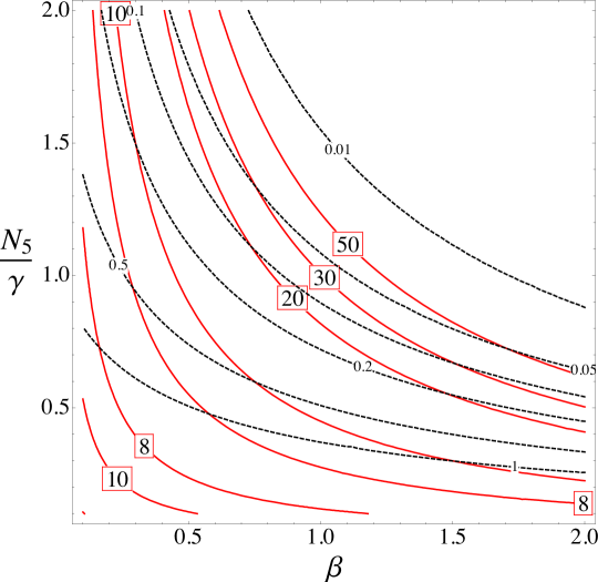
Figure 2: The lines of constant lattice spacing in units of the string tension $a_{4}\sqrt{\sigma}$ are shown as dashed black lines in the plane ($\beta,N_{5}/\gamma$). The lines of constant scalar mass in units of the string tension $m_{5}/\sqrt{\sigma}$ are shown with solid red lines. This plot is similar to the drawing in Fig.7 of Ref. [13], where the authors also took into account the features of the phase diagram which we will describe in Sec. 4 (note that the coordinate $\beta$ is called $\beta_{5}$ in Ref. [13], and $N_{5}/\gamma$ is called $\tilde{N}_{5}$).

Keeping this in mind and assuming that Fig. 2 represents the actual lines of constant physics, we can speculate about how to reach a continuum limit for this lattice model. As it was firstly noted in Ref. [13], two different four–dimensional continuum theories can be described as the lattice spacing $a_{4}$ vanishes. The one we are interested in for this study is a ${\rm SU(}2{\rm)}$ Yang–Mills theory coupled to an adjoint scalar field: this theory is described by the lattice model following a line of constant $m_{5}/\sqrt{\sigma}$ (one of the solid red lines in Fig. 2) towards smaller values of $\beta$ and bigger values of $N_{5}/\gamma$. In this direction, $a_{4}\sqrt{\sigma}$ decreases, while the scalar mass is kept fixed, and the effects of the regularization are suppressed by powers of $a_{4}\sqrt{\sigma}$. A remarkable feature of this approach to the continuum limit is that the direction to be taken in the bare parameter space goes towards higher values of $N_{5}/\gamma$. This means that the size of the extra dimension $2\pi R$ increases in units of the lattice spacing $a_{4}$, while the theory dimensionally reduces to four dimensions as already suggested in the D–theory non–perturbative approach to quantum field theories [20, 21].
Let us stress again that Eq. (23) to Eq. (25) are found using one–loop continuum perturbative results and tree–level relations between the lattice parameters and the continuum ones. The lines of constant values for the cut–off $1/a_{4}\sqrt{\sigma}$ and for the scalar mass $m_{5}/\sqrt{\sigma}$ must be determined non–perturbatively using numerical simulations, and we shall see if and how they deviate from the perturbative expectations. In particular, it would be interesting to see if the hierarchy between the scalar mass and the string tension still holds at stronger couplings.

4 The phase diagram

In this section, we briefly describe a further issue arising in the study of the lattice model. Indeed, the perturbative predictions we referred to in Sec. 3 do not take into account the rich phase structure of the lattice theory. Since it is crucial for our purposes to simulate the theory in the correct phase, let us first discuss the current understanding of the phase diagram of the ${\rm SU(}2{\rm)}$ pure gauge theory in five dimensions described by the action in Eq. (4).
The first feature, which was already investigated in the early studies in Ref. [16], concerns the lattice model on the line $\beta_{4}=\beta_{5}$, or equivalently $\gamma=1$. This isotropic model, where the lattice spacings are the same, $a_{4}=a_{5}$, has a bulk phase transition when all the dimensions are equal. This phase transition is independent of the physical volume of the system; it is signalled by a sudden jump of the plaquette expectation value and by a hysteresis cycle. The bulk line separates a confined phase that is connected to the strong coupling regime from a Coulomb–like phase connected to the weak coupling regime. An interesting feature of the isotropic model is that the bulk transition disappears when the lattice size in any one dimension is decreased below a critical size, $L_{c}$, which is the critical length of the Polyakov loop in that direction. Below $L_{c}$ centre symmetry is broken. In this case the phase transition becomes a second order one in the same universality class of the four–dimensional Ising model: the position of the critical point scales with the four–dimensional volume and with the number of sites $N_{5}$ in the extra dimension. This has been verified numerically for $N_{5}=2$ with a Binder cumulant finite–size scaling in Ref. [13]. We have performed a scaling analysis of the susceptibility of the Polyakov loop in the compact direction $L_{5}$, and obtained compatible results. However, when the number of points in the compact fifth dimension is increased to $N_{5}=4$, we could not locate the second order phase transition before hitting again the bulk transition; this is true up to $N_{4}=14$, which is the biggest lattice we explored at $\gamma=1$. A bigger aspect ratio $N_{4}/N_{5}$ is probably needed at $\gamma=1$ in order to see the effects of the compactification (namely a thermal–like second order phase transition), our computational resources did not allow us to further explore this issue. A very recent study of the phase diagram at very small anisotropies $\gamma<1$ was presented in Ref. [14] and the authors claim that if any one of the dimensions becomes smaller than a minimal lattice size $L^{\rm min}(\gamma)$, no sign of the bulk phase transition can be detected. At $\gamma=1$, their simulations hint at $2<L^{\rm min}<6$, and the results are also supported by Ref. [15].
In the following, we are interested in the region of the parameter space where $\gamma>1$. Clearly, in this case $a_{4}>a_{5}$, and hence the extra dimension can be easily made small enough to obtain dimensional reduction as described above. The phase diagram in this region is known at $N_{5}=4$ and $N_{5}=6$ [11]. We performed a similar study on bigger four–dimensional lattices and obtained compatible results. We want to stress that our aim is not to study the details of these phase transitions; therefore we simply determined the critical lines in the parameter space searching for the location of the peak in the susceptibility of the compact Polyakov loop. As shown in Fig. 3 our results compare favourably to Ref. [11], which also provides a cross–check of the validity of our simulation code.

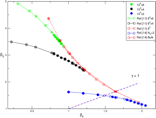
Figure 3: Phase diagram of the five–dimensional ${\rm SU(}2{\rm)}$ pure gauge lattice model. In red we report the position of the bulk phase transition characteristic of the system with no compact dimensions. Both results from Ref. [11], and from Ref. [14], are shown. Moreover, we report the lines of second order phase transition at $N_{5}=2$ (blue), $N_{5}=4$ (black) and $N_{5}=6$ (green). Our results are plotted with filled circles and come from simulations on the lattices shown in the legend of the plot. They are compatible with other results in the literature.

The main feature of the phase diagram in this region is that, for fixed $N_{5}$, there is a line of second order phase transition that merges into the bulk one as the anisotropy is decreased below a critical value $\gamma_{c}$. Above this $\gamma_{c}$, which depends on $N_{5}$, the transition line separates a phase where the centre symmetry in the extra compact direction is not broken (at smaller $\beta_{5}$) from the phase where the symmetry is broken and the compact Polyakov loop acquires a non–zero expectation value. We refer to this phase as the dimensionally reduced one, following the terminology in Ref. [13]. However, for $\gamma<\gamma_{c}$ the bulk phase transition line separates a confined phase (at smaller $\beta_{4}$) from a Coulomb–like phase extending to the weak–coupling regime, exactly as we described in the isotropic case. This pattern of phase transitions is shown in Fig. 4 using the data already shown in Fig. 3, but now separating the phase diagram at $N_{5}=4$ from the one at $N_{5}=6$. Since the second order phase transition is physical, its location changes as we change $N_{5}$. Note also that, at fixed $N_{5}$, there is no sign of a bulk phase transition for $\gamma>\gamma_{c}$. The emerging physical picture tells us that the disappearance of the bulk phase transition happens when the five–dimensional system compactifies; in other words, $\gamma_{c}$ defines a critical lattice spacing in the extra dimension $a_{5c}$ such that $L_{5c}=a_{5c}N_{5}$.

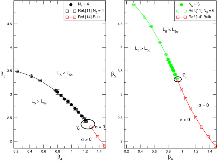
Figure 4: Phase diagram of the five–dimensional ${\rm SU(}2{\rm)}$ pure gauge lattice model in the ($\beta_{4},\beta_{5}$) plane for different values of $N_{5}$. The data are the same as in Fig. 3. The bulk phase transition separating a confined from a Coulomb–like phase disappears for $\gamma>\gamma_{c}$ into a physical thermal–like phase transition. The location of this transition changes in the parameter space as we change $N_{5}$. The region we are interested in studying is the one labelled by $L_{5}<L_{5c}$.

Ref. [11] presents estimates for $\gamma_{c}$, for both $N_{5}=4$ and $N_{5}=6$, and for the renormalized anisotropy $\xi$ in those points, so that the critical radius $R_{c}$ of the extra dimension in units of the four–dimensional lattice spacing can be computed. The data in Ref. [11] suggest that $L_{5c}\sim 2.25a_{4}$ for $N_{5}=4$, and $L_{5c}\sim 2.16a_{4}$ for $N_{5}=6$: for extra dimensions bigger than these approximate values, the system shows a bulk phase transition characteristic of the five–dimensional model. The interesting region for our purposes, is at $\gamma>\gamma_{c}$ and above the line of second order phase transition, where the extra dimension is smaller than its critical value $L_{5}<L_{5c}$.

5 Lines of constant physics

Strategy of lattice simulations

Our main goal is to study whether a light scalar particle does exist in the low–energy spectrum of the five–dimensional theory. The strategy of the simulations is very straightforward in principle. The lattice model we described in Sec. 2 has four tunable parameters: the two coupling constants $\beta_{4}$ and $\beta_{5}$, and the number of sites $N_{5}$ and $N_{4}$. If we assume, for the moment, that the spectrum does not depend on $N_{4}$ (e.g. we are in the infinite volume limit of the lattice theory), we are left with three parameters. Fixing the bare coupling constants dynamically determines the two lattice spacings, whereas fixing $N_{5}$ determines the length of the extra dimension. In other words, by fixing a point in this three–dimensional bare parameter space, we are choosing a system with a given separation of scales between the ultra–violet cut–off $\Lambda_{\rm UV}$, the compactification scale $\Lambda_{\rm R}$ and the scalar mass $m_{5}$ (all the energy scales are again expressed in units of the string tension).
The three energy scales of the system can only be determined a posteriori by measuring physical observables with numerical Monte Carlo simulations.
Let us focus first on the determination of the cut–off scale. From Eq. (18) it is clear that a measure of the four–dimensional string tension in units of the lattice spacing yields the separation between the low-energy scale and the cut–off. The string tension $\sqrt{\sigma}$ in units of the four dimensional lattice spacing $a_{4}$ can be extracted using different observables. We choose to measure correlation functions of Polyakov loops winding around the three spatial directions: the string tension can then be extracted from the mass of the lightest state that propagates.
The non–perturbative scalar mass instead can be obtained from the ratio of two lattice observables as expressed in Eq. (20). Having obtained the string tension, we only need to measure $m_{5}$ in units of the lattice spacing $a_{4}$. Since it is the mass of a scalar particle, we use correlation functions of operators that only project on the $0^{++}$ representation of the symmetry group of the cube (with positive parity and charge) following standard spectroscopic notation. Due to the presence of the extra dimension, different types of basis operators can be used in the correlation functions; in particular we distinguish those created using Polyakov loops wrapping around the compact fifth dimension from those created using Wilson loops embedded in the three large spatial directions. We generically refer to the first kind of operators as the scalar ones, while the second set is referred to as glueballs. In the following, we will focus mostly on masses extracted from correlators of the scalar operators, but part of our analysis will be dedicated to glueballs as well. In this respect, we greatly improve the exploration of the scalar spectrum as first presented in Ref. [13]. More details on the operators and on the noise–reduction techniques we used are given in the Appendix.
The last scale we need to set is the compactification scale $\Lambda_{\rm R}$; unfortunately, we were not able to measure a third independent observable that could be used for this purpose. In particular, we would need a measure of the extra dimensional lattice spacing $a_{5}$ that needs to be done in the confined phase. However this problem can be easily overcome. As we noted in Eq. (21), the separation between the cut–off and the compactification scale is determined, at leading order, by the bare parameters of the lattice model. Therefore, knowing $\Lambda_{\rm UV}$ from a measure of $a_{4}\sqrt{\sigma}$ at one point $(\beta_{4},\beta_{5},N_{5})$ is sufficient to approximately estimate $\Lambda_{\rm R}$. As we already mentioned, the last step of Eq. (21) is only valid in the weak–coupling limit that is reached, at fixed $\gamma$, when $\beta\rightarrow\infty$. Although this seems like a reasonable approximation in Ref. [13] where the values of $\beta$ are large, we try to estimate the systematic deviation of $\frac{\Lambda_{\rm UV}}{\Lambda_{\rm R}}$ from its tree–level value $\frac{N_{5}}{\gamma}$. As we will show in the following, our simulations are performed in a different region of the phase diagram with respect to Ref. [13] and our $\beta$ values are smaller.

$\xi=a\gamma^{2}+b\gamma+c$
$a$	$b$	$c$	$\tilde{\chi}^{2}$
–	1.600(15)	-0.446(37)	0.61
-0.03(1)	1.767(62)	-0.641(76)	0.32
-0.06(1)	1.950(45)	$1-a-b$	0.77

Table 1: Parameters of the fitted function $\xi=\xi(\gamma)$. The all range of data was used, from $\gamma\sim 1.224$ to $\gamma=4$.

We expect corrections to Eq. (13) due to quantum fluctuations. Since the non–perturbative relation between the bare anisotropy $\gamma$ and the renormalized one $\xi$ had already been studied for this system, we interpolated the data available in Ref. [11], in order to estimate the ratio $\frac{\Lambda_{\rm UV}}{\Lambda_{\rm R}}$ for the points we simulated. The relation $\xi=\xi(\gamma)$ is shown in Fig. 5.

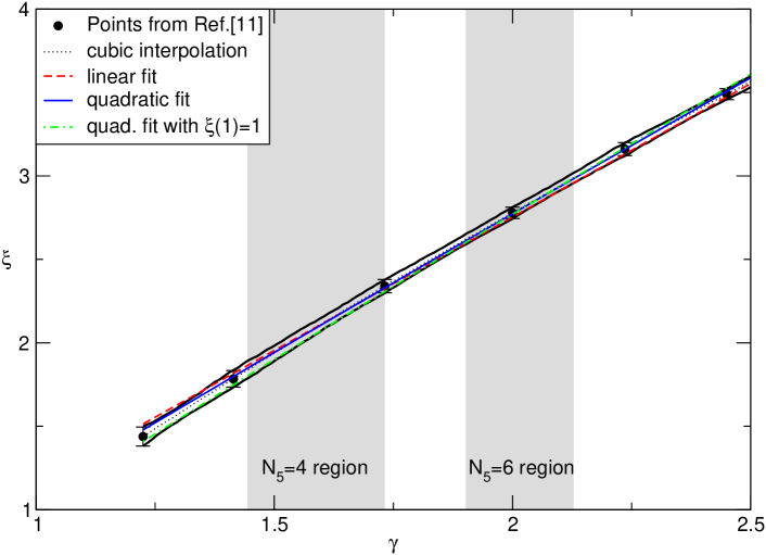
Figure 5: The relation $\gamma\sim\xi$ is corrected by quantum fluctuations. We interpolated data from Ref. [11] that were obtained by measuring $\xi$ non–perturbatively using ratios of suitable correlation functions. All the data are in the correct phase where $\sqrt{\sigma}\neq 0$. In the plot we show three different fits (with $\tilde{\chi}^{2}\sim 0.5-0.7$) and the interpolation used to obtain $\xi$ in the regions where we performed the simulations (both for $N_{5}=4$ and for $N_{5}=6$). They all compare well and are hardly distinguishable.

We performed three different fits of the data: a linear fit, a quadratic one, and a quadratic fit imposing $\xi(1)=1$. The details of the fits are summarised in Tab. 1. In practice, to obtain $\xi$ for the points in our simulations, we used a cubic interpolation nested inside a bootstrap procedure for the errors. The result is again shown in Fig. 5 together with the $1$–$\sigma$ contour. The errors are such that all the lower order fits are compatible with this interpolation. Although we only use interpolated values of $\xi$, it must be noted that $\xi=\xi(\gamma)$ could in principle also depend on the other bare parameter $\beta$. However, in the region where $\xi$ was initially measured non–perturbatively, the value of $\xi$ is shown to be fairly insensitive to the values of $\beta$ (cfr. Fig. 1 in Ref. [11]). This is true in particular for the values of $\xi$ that we are going to use, namely $1.7\leq\xi\leq 3.0$. We performed our simulations at $\beta$ values that are inside (or just slightly off) the region where $\xi$ was observed to be independent of it. Hence we expect the systematic errors of this interpolation procedure to be under control.
Before showing the details of the simulations and the results, let us summarize the main steps of this study:

1. we fix a point in the three–dimensional parameter space $(\beta_{4},\beta_{5},N_{5})$ that is in the dimensionally reduced phase;

2. on this point we measure $a_{4}\sqrt{\sigma}$ and $a_{4}m_{5}$ from correlation functions of suitable operators;

3. the measured observables determine the cut–off scale and the scalar mass from Eq. (18) and Eq. (20);

4. we use the available data for $\xi$ to estimate the compactification scale using Eq. (21) and the measured cut–off scale (this yields a better determination of the anisotropy than the one coming from tree–level relation $\gamma=\xi$, and allows us to estimate the errors due to $\beta\neq\infty$);

5. we then move to a different point $(\beta_{4},\beta_{5},N_{5})$ and repeat the procedure;

6. having done this for a certain number of points allows us to study the dependence of the energy scales on the bare parameters and to determine lines of constant physics;

7. more importantly, this allows us to study the behaviour of $m_{5}$ as a function of $\Lambda_{\rm UV}$ or $\Lambda_{\rm R}$ and to disentangle cut–off effects from compactification effects.

Results from lattice simulations

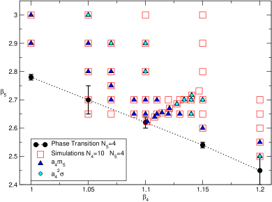
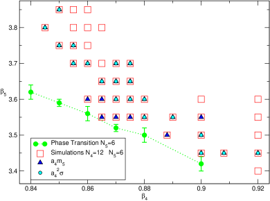
(a)	(b)

Figure 6: The plots show the region of the phase diagram that we explored with numerical simulations, both for $N_{5}=4$ (a) and $N_{5}=6$ (b). The location of the second order phase transition is also shown. The blue squares are points where the scalar mass $a_{4}m_{5}$ was reliably extracted, whereas the green circles represent points where we were able to measure the string tension $a_{4}\sqrt{\sigma}$.

We performed simulations at two different values of $N_{5}$ and several different four–dimensional volumes. The smaller lattice has $N_{4}=10$ and $N_{5}=4$. This volume is also the one we used to locate the position of the second order phase transition in the left panel of Fig. 4. On this lattice, we generated $\mathcal{O}(800000)$ configurations and the correlators of the interesting observables were binned over $20$ configurations after thermalization. We chose a wide range of values for $\beta_{4}$ and for $\beta_{5}$, starting very close to the line of second order phase transition. In this region we expect a light scalar in units of the lattice spacing because the scalar mass is the inverse of the correlation length, and the latter diverges at the critical point. From the phase structure discussed above, we also expect to find a finite string tension. The details of the simulated points on this volume are reported in Tab. 3.
Similarly, for $N_{5}=6$ we simulated on lattices with $N_{4}=12$, generating $\mathcal{O}(600000)$ configurations, binning the observables over $20$ configurations. The parameters of the simulations on this second volume are summarised in Tab. 4. In the tables we show both the bare parameters that fix the location of the point in the phase diagram, and the values of $\gamma$ and the corresponding interpolated value of $\xi$. The size of the non–perturbative effects on the anisotropy can be extracted from these numbers. Moreover, from the same tables, one can compare the separation of scales in Eq. (21) to the naive estimate using the bare parameters, i.e. $\frac{N_{5}}{\gamma}$. What we notice is that the naive expectation is systematically larger than what is obtained by measuring the anisotropy non–perturbatively. As a result, we were only able to explore the following range

$$1.7\;\lesssim\;\frac{N_{5}}{\xi}=\frac{\Lambda_{\rm UV}}{\Lambda_{\rm R}}=\frac{2\pi R}{a_{4}}\;\lesssim\;2.3\;,$$ (26)

where the upper limit is close to the critical value $L_{5c}/a_{4}\sim 2.16-2.25$ that we identified in Sec. 4.
Since this is the first time that this particular region of the phase space is explored with lattice simulations, we performed a broad scan, aiming primarily at identifying the interesting region. As a consequence, there are lattices for which we were unable to measure precisely both the string tension and the scalar mass. In Fig. 6, we show all the points reported in Tab. 3 and in Tab. 4, but at the same time we identify the ones where either $a_{4}m_{5}$ or $a_{4}\sqrt{\sigma}$ could not be extracted satisfactorily.

Our lattice data suggest that the lattice spacing $a_{4}$ changes dramatically in these regions of the phase space. As shown in Fig. 6, the string tension $a_{4}\sqrt{\sigma}$ can only be measured in a small subset of points; the points closer to the line of second order phase transition are characterized by spatial Polyakov loops whose mass is too high for a signal to be extracted reliably. Since the mass of the loops is given by $N_{4}a_{4}\sigma$, we see that in this region the lattice spacing $a_{4}$ is getting larger in units of the string tension. Following our discussion in Sec. 3, we regard the region close to the phase transition line as the one characterized by a small cut–off $\Lambda_{\rm UV}$. In this region, there is not a clear separation between the low–energy physics and the cut–off, and we expect to observe large discretization errors. To make things even more interesting, we find the scalar mass $a_{4}m_{5}$ to be small in this same region, where $a_{4}$ is large. In fact, it turns out to be very difficult to find points in the phase diagram where both $\sqrt{\sigma}$ and $m_{5}$ are separated from the cut–off scale at the same time. This results in a scalar mass $m_{5}\gtrsim\sqrt{\sigma}$ for all the points on which we were able to reliably measure the string tension, indicating the same hierarchy expected from perturbation theory (cfr. Fig. 2). On the other hand, a light non–perturbative scalar does exist very close to the second order transition line, where $a_{4}m_{5}$ is small and $a_{4}\sqrt{\sigma}$ is large.

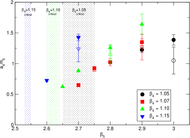
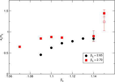
(a)	(b)

Figure 7: (a) The scalar mass in units of the lattice spacing $a_{4}m_{5}$ as a function of $\beta_{5}$ and for four different values of $\beta_{4}$ at $N_{5}=4$. The approximate location of the critical region is shown by the shaded regions for the different values of $\beta$. (b) At fixed $\beta_{5}$, we show the behaviour of $a_{4}m_{5}$. Smaller values of $\beta_{4}$ are closer to the phase transition line, but we do not have an estimate of its location in this direction. Open symbols correspond to alternative fitting ranges in the effective mass plateaux for the scalar state (see Appendix). When not quoted, errors are smaller than symbols.

A more quantitative statement can be made by looking at the measured observables as functions of the bare parameters. For example, our data allow us to study the behaviour of $a_{4}\sqrt{\sigma}$ at fixed value of $\beta_{4}$ as we change $\beta_{5}$, and vice versa. The same can be done with $a_{4}m_{5}$ and therefore with the ratio $m_{5}/\sqrt{\sigma}$. In Fig. 7(a) we select four different values of $\beta_{4}$ and we plot the mass $a_{4}m_{5}$ obtained from scalar operators as a function of $\beta_{5}$. Fig. 7(b) shows the dependence of the scalar mass as a function of $\beta_{4}$ for fixed $\beta_{5}$. The values of $a_{4}m_{5}$ are taken from Tab. 5 where we summarise our results for $N_{5}=4$, whereas we report the results for $N_{5}=6$ in Tab. 7. As we have already mentioned, we notice that the scalar mass approaches the cut–off scale $a_{4}m_{5}\gtrsim 1$ as we move away from the line of second order phase transition. This happens both in the $\beta_{4}$ and $\beta_{5}$ directions. Similarly, following Ref. [13], we can move in the parameter space along a line of fixed $\gamma$, while changing $\beta$. We choose $\gamma\approx 1.54$ in order to obtain a separation of scales $\Lambda_{\rm UV}/\Lambda_{\rm R}\approx 2$ after taking into account the renormalized anisotropy. In the interval $\beta\in[1.71,\;1.77]$, we accurately study the low–lying spectrum of scalar particles employing our larger set of operators with the inclusion of glueballs. Using a variational method, detailed in the Appendix, we studied the operator content of the different mass eigenstates in the scalar channel. We extracted the mass of the scalar ground state and its first excitation. The resulting masses are shown in Fig. 8, where we compare the non–perturbative scalar masses calculated via the variational ansatz with the masses obtained solely from effective mass plateaux of scalar operators. It is clear from the results in the plot that a variational analysis is crucial to identify the lightest scalar state as $\beta$ is increased.
Further information can be obtained by studying the change in the operator content of the scalar eigenstates as $\beta$ increases. We measure the normalized projection of the mass eigenstates onto each operator used in the correlation matrix. The projection of the extracted ground state is shown in Fig. 9. The plot clearly shows how the contribution of the scalar operators to the ground state decreases as $\beta$ increases. At higher values of $\beta$, glueball operators have a larger overlap onto the ground state. On the other hand, we clearly see that at lower values of $\beta$, closer to the line of second order phase transition, the scalar state has a dominant contribution from the extra–dimensional operators.
The relative mixing of the first excited state onto the operators in the variational set is shown in Fig. 10. The points where the mixing is calculated are the same as in Fig. 9. Up to $\beta=1.75$, the first excited state is dominated by a projection onto the scalar operators, suggesting an extra–dimensional nature for this particle.
Again, we conclude that the scalar mass becomes heavy in units of the cut–off scale while moving away from the critical line, as shown in Fig. 8. This suggests that at $\beta\gtrsim 1.77$ for $N_{5}=4$ the scalar particle becomes heavy; from data in Ref. [13] taken at $1.83\leq\beta\leq 1.91$ at the same $N_{5}$ (but at $\gamma=2$) it can be shown that $m_{5}\gtrsim 2\Lambda_{\rm UV}$ and therefore the scalar particle cannot be considered a low–energy degree of freedom of the theory.

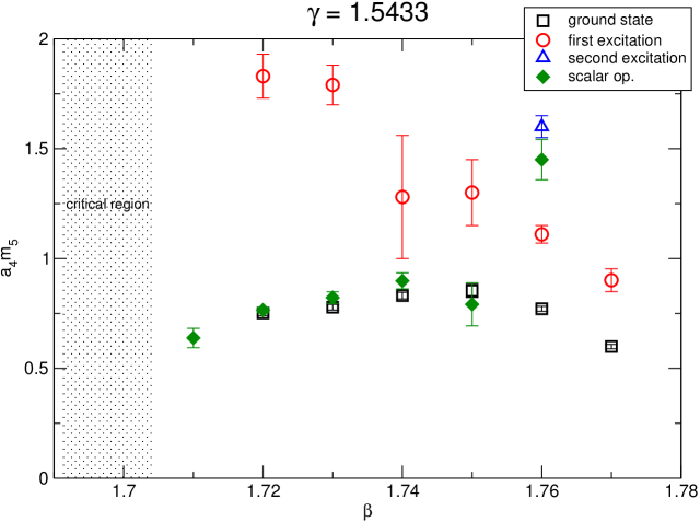
Figure 8: The scalar mass in units of the lattice spacing $a_{4}m_{5}$ as a function of $\beta$ for a fixed value of $\gamma=1.5433$. The shaded area is the approximate location of the second order phase transition. Open symbols refer to masses obtained from a variational procedure. Filled symbols are masses extracted from diagonal correlators of scalar operators.

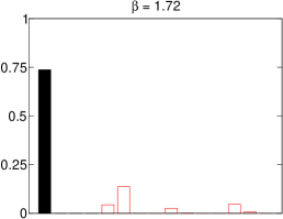
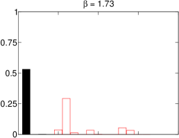
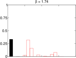
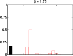
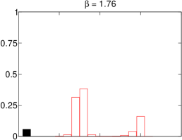
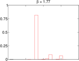
Figure 9: Relative projection of the ground state onto each of the operators in the variational set. Filled symbols correspond to the set of smeared scalar operators, whereas the open symbols refer to the smeared versions of glueball operators.

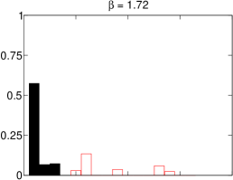
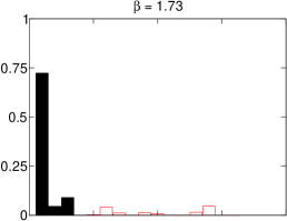
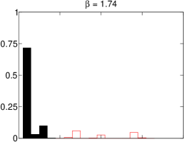
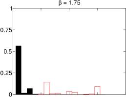
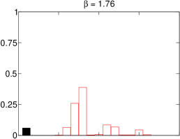
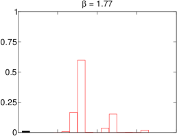
Figure 10: Relative projection of the first excited state onto each of the operators in the variational set. Filled symbols correspond to the set of smeared scalar operators, whereas the open symbols refer to the smeared versions of glueball operators.

While the scalar mass becomes smaller as we approach the critical line, the opposite happens to the string tension. Its behaviour in bare parameter space is best illustrated by the data at $N_{5}=6$. All the points where we were able to extract the string tension $a_{4}\sqrt{\sigma}$ are summarized in Tab. 6 for $N_{5}=4$, and Tab. 8 for $N_{5}=6$. In Fig. 11(a) the string tension is shown at three different values of $\beta_{4}$: the common feature of the data is that the string tension increases as the critical line is approached. As discussed above, this behaviour can be interpreted as an increase of the lattice spacing $a_{4}$ in units of the physical string tension $\sqrt{\sigma}$. A similar functional dependence of $a_{4}\sqrt{\sigma}$ is shown in Fig. 11(b), where $\beta_{5}$ is fixed. At lower values of $\beta_{4}$, closer to the line of phase transition, the string tension grows and it becomes very difficult to extract a signal from our numerical simulations. We can easily infer from the data that the string tension will decrease with increasing $\beta$ at fixed $\gamma$, as already reported in Ref. [13]. This behaviour is expected since $\beta\rightarrow\infty$ is the weak–coupling limit of the theory, and accordingly the string tension should vanish.

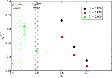
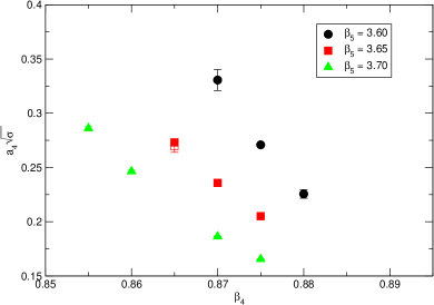
(a)	(b)

Figure 11: (a) The string tension in units of the lattice spacing $a_{4}\sqrt{\sigma}$ as a function of $\beta_{5}$ and for three different values of $\beta_{4}$ at $N_{5}=6$. The approximate location of the critical region is shown for the different $\beta_{4}$. (b) At fixed $\beta_{5}$, we show the behaviour of $a_{4}\sqrt{\sigma}$. Smaller values of $\beta_{4}$ are closer to the phase transition line, but we do not have an estimate of its location in this direction. Open symbols correspond to alternative fitting ranges in the effective mass plateaux for the torelon state (see Appendix). When not quoted, errors are smaller than symbols.

From the previous discussion we have identified the lines of constant physics in the phase diagram at fixed $N_{5}$. Moreover, we find similar features by going from $N_{5}=4$ to $N_{5}=6$. The lines of constant cut–off $\Lambda_{\rm UV}$ are represented by contour lines of $a_{4}\sqrt{\sigma}$. These lines start close to the line of second order phase transition for $\gamma\sim\gamma_{c}$, but then move away from it as $\gamma$ is increased. To summarize, at fixed $\gamma$, the lowest $\beta$ corresponds to the lowest $\Lambda_{\rm UV}$; a larger separation between the low–energy physics and the cut–off is found at bigger values of $\beta$, and this is the region where the lattice discretization starts to become irrelevant and we can safely extract the low–energy physics from numerical simulations (cfr. Eq. (15)). What we are really interested in is the behaviour of the scalar mass $m_{5}$ in units of the string tension $\sqrt{\sigma}$. By looking at the ratio of $a_{4}m_{5}$ over $a_{4}\sqrt{\sigma}$, we can deduce the lines of constant scalar mass. Unfortunately, we cannot use all the measured values of $a_{4}m_{5}$, because we also need a measure of $a_{4}\sqrt{\sigma}$ on the same point. The general pattern of these lines is again quite clear: the lightest scalar is found closer to the second order critical line, but it soon starts decoupling from the low–energy physics as we move away from it. There is only a small patch of the phase space we explored where Eq. (14), Eq. (15) and Eq. (16) hold simultaneously. The lightest mass $m_{5}$ we measured is of order $2\sqrt{\sigma}$.
Using the non–perturbative lines of constant physics, we can try to discuss the different types of continuum limit. Our findings can be compared with the perturbative picture reported in Ref. [13], bearing in mind that our results are obtained for fixed values of $N_{5}$ and $N_{4}$ and therefore could be affected by finite–volume effects. For this comparison, we shall refer in particular to Fig. 7 of Ref. [13]. First let us relate our choice of parameters with the definitions in Ref. [13]: the horizontal axis in Fig. 7, is labelled by $\beta_{5}$, which corresponds to what we call $\beta$ (cfr. Eq. (8)) in this work; the vertical axis is labelled by $\tilde{N}_{5}$, which is defined as $N_{5}/\gamma$. In the following we use only our parametrization, and the reader should refer to the discussion above for any comparison. At any fixed value for $\beta_{4}$ in the dimensionally reduced phase, there is a lower bound for $\beta_{5}$, given by the location of the critical point. By increasing $\beta_{5}$, we cross lines of decreasing lattice spacing $a_{4}$, therefore moving towards a continuum limit, meaning that the lattice discretization effects vanish. At the same time we cross lines of increasing scalar mass $m_{5}$, which inevitably decouples from the low–energy spectrum: the low–energy effective theory described in this region is four–dimensional, and contains only gauge degrees of freedom. A similar limit occurs at fixed $\beta_{5}$ and increasing $\beta_{4}$. However, by following a line of constant scalar mass in the phase diagram, we cross lines of different fixed lattice spacing. In particular, moving towards smaller $\beta_{4}$ and bigger $\beta_{5}$ the lattice spacing decreases, allowing us to reach the desired separation between the cut–off and the low–energy physics with a constant value of the scalar mass. The low–energy dynamics is then described by an effective four–dimensional theory with a light adjoint scalar in the low–energy spectrum, having started with a five–dimensional theory with only gauge degrees of freedom. This being an effective description, it is expected to hold only up to the energy scales given by the compactification radius, as we already mentioned in Sec. 3. What we have learned from our non–perturbative map of the energy scales in the phase diagram of the lattice model is that it requires a certain amount of fine tuning to pin down the location of a line of constant mass and to follow it. Moreover, the behaviour of the cut–off scale near to the line of second order phase transition (cfr. Fig. 11) makes it very difficult to determine $\frac{m_{5}}{\sqrt{\sigma}}$ non–perturbatively, thereby limiting our ability to reach values of the scalar mass that are smaller than the square root of the string tension. This is an important result for future studies in this context, and it was not anticipated before using perturbative arguments. For example, looking at the perturbative results in Fig. 2, or equivalently at Fig. 7 in Ref. [13], where the line of phase transitions in the $a_{5}\rightarrow 0$ is taken into account, we note that the lines of fixed $a_{4}\sqrt{\sigma}$ go straight into the critical line. This behaviour is not supported by our non–perturbative results: those lines cannot cross the point where the phase transition occurs, because $a_{4}\sqrt{\sigma}$ increases as we approach that point. Any attempt to follow a line of constant scalar mass would have to deal with this problem.

Compactification effects on the scalar mass

So far we have only explored the behaviour of energy scales in the bare parameter space. However, each point we have simulated on the phase diagram corresponds to a precise location in the space given by the three energy scales we are interested in, that are $\Lambda_{\rm UV}$, $\Lambda_{\rm R}$ and $m_{5}$. We can therefore translate our results at $N_{5}=4$ and $N_{5}=6$ into a common set of points $(\Lambda_{\rm UV},\Lambda_{\rm R},m_{5})$. This approach allows us to study $m_{5}$ as a function of the other two energy scales, instead of the bare parameters. From now on we express the energies $\Lambda_{\rm UV}$ and $\Lambda_{\rm R}$ using their length counterpart, $a_{4}\sqrt{\sigma}$ and $R\sqrt{\sigma}$ respectively. These two length scales are related to each other by Eq. (21) and they are both measured non–perturbatively: the first is directly measured, whereas the second relies on the interpolated data of $\xi$ from Ref. [11].
The range of values of $a_{4}\sqrt{\sigma}$ and $R\sqrt{\sigma}$ spanned in our simulations is shown in Fig. 12, and the data we used are summarized in Tab. 9 and Tab. 10. In the following plots, we report results from $N_{5}=4$ together with the ones from $N_{5}=6$. When more than one value for $a_{4}\sqrt{\sigma}$ or $a_{4}m_{5}$ is extracted for the same $(\beta_{4},\beta_{5})$ point, we apply the following procedure: if the values are compatible within one standard deviation, we plot the weighted average as central value, and the weighted error as the statistical error; we also use the spread of the results to estimate the systematic error due to the choice of the effective mass plateaux. If the values are not compatible, we use the average for the central value, whereas the systematic error is chosen to comprise both the lowest and the highest values.
With our available data, we can explore the behaviour of the scalar mass $m_{5}$ in the following region of lattice spacing $a_{4}$

$$0.15\;<\;a_{4}\sqrt{\sigma}\;<\;0.40\;,$$ (27)

and compactification radius $R$

$$0.05\;<\;R\sqrt{\sigma}\;<\;0.12\;.$$ (28)

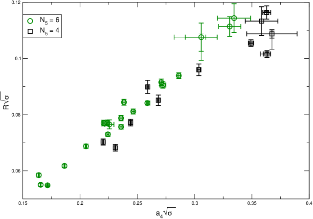
Figure 12: The points in the phase space are mapped into the physical space of the energy scales of the system. In the plot we report the length scale corresponding to the ultra–violet cut–off, and the one corresponding to the compactification energy. Using both data from $N_{5}=4$ and $N_{5}=6$, we can span a larger region of this space. Some points have two different type of error bars described in the text: the thicker one is statistical, whereas the thinner is systematic.

The major advantage of interpreting the data in terms of these physical quantities is that we can disentangle compactification effects from cut–off effects. It is clear from Fig. 12 that we have points at different values of the lattice spacing, but at the same value of the compactification radius. The scalar mass on those particular points can therefore be studied at fixed compactification scale and different cut–off scale. On the other hand, we also have points at the same value of the lattice spacing, but at different radii, which can be used to study the behaviour of the scalar mass at fixed cut–off scale. From Fig. 12 we can also infer that increasing $N_{5}$ would allow us to explore a wider range of cut–off values for fixed compactification scale.
Our main goal is to clarify the validity of the result in Eq. (1) where the perturbative scalar mass is expected to depend strongly on the compactification scale. In our lattice model we would like to see if there are leading cut–off corrections to this expected behaviour when we look at the non–perturbatively measured scalar mass. The simplest way of looking for these corrections is to study the dependence of the scalar mass on the lattice spacing. However, our values for the lattice spacing usually correspond to different values of the compactification radius. It is clear from this discussion that the study in Ref. [13] cannot give any hints about Eq. (1): the lattice spacing always changes together with the compactification radius, because their ratio is forced to be constant. Nothing can be said about the dependence of $m_{5}$ at fixed compactification scale nor at fixed cut–off scale from the results of these earlier studies. Using our data, we can plot $m_{5}$ as a function of $a_{4}$ and separately as a function of $R$. The plots are shown in Fig. 13: Fig. 13(a) shows the scalar mass dependence on the lattice spacing in the range defined in Eq. (27), whereas Fig. 13(b) shows its behaviour as a function of the compactification radius in the range of Eq. (28). The observed range for the scalar mass in units of the string tension is

$$2\;<\;\frac{m_{5}}{\sqrt{\sigma}}\;<\;10\;.$$ (29)

The important thing to notice in this analysis is how the scalar mass changes between the two plots. While some of the points are insensitive to the two different choices of variables, it is striking to see points with the same mass but far away in Fig. 13(a) fall on top of each other once expressed in terms of the compactification radius in Fig. 13(b). If Eq. (1) holds, then the combination $m_{5}R$ should be independent of $R$ at leading order, while retaining any dependence on the cut–off $a_{4}$. In order to separate the scalar particle from the Kaluza–Klein modes, this variable should be less than one as we stated in Eq. (16). In Fig. 14 we plot $m_{5}R$ as a function of $a_{4}\sqrt{\sigma}$. The data show a scalar mass in units of the compactification radius in the range

$$0.2\;<\;m_{5}R\;<\;0.5\;.$$ (30)

Such range is smaller than the one spanned by $m_{5}/\sqrt{\sigma}$ by a factor of $2$ for the same interval of lattice spacings. This evidence support the observation that the dependence on $a_{4}\sqrt{\sigma}$ is milder than the one shown in Fig. 13(a) and it is compatible with the perturbative expectation in Eq. (1). The product $m_{5}R$ does not show any sign of quadratic divergences as the lattice spacing is reduced. However, we must recall that all the simulations were performed on a fixed value of $N_{4}$, therefore the points at the smallest values of $a_{4}\sqrt{\sigma}$ are the ones on the smallest physical volumes and finite–size effects could be present. On the other hand, large values of $a_{4}\sqrt{\sigma}$ point in the direction of larger discretization effects.

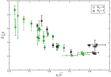
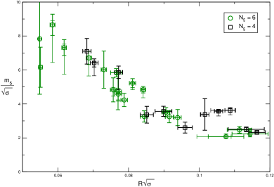
(a)	(b)

Figure 13: (a) The scalar mass as a function of the lattice spacing for $N_{5}=4$ and $N_{5}=6$; (b) The same scalar mass is also shown as a function of the compactification radius. Points at the same value of the radius have the same mass within the statistical error. Each of the point in (a) corresponds to a point in (b). Systematic errors due to the choice of the effective mass plateaux are reported for some points using thinner error bars.

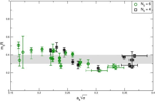
Figure 14: The scalar mass in units of the compactification radius $m_{5}R$ is shown to be mildly dependent on the lattice spacing $a_{4}\sqrt{\sigma}$. The grey band $0.3\leq m_{5}R\leq 0.4$ includes all points within two standard deviations and it is drawn to guide the eye. Also in this case, systematic errors are shown with thinner error bars, whereas the thicker ones represent statistical standard deviations.

6 Conclusions

Lattice theories in more than four dimensions prove to be very interesting. They provide a sensible and well–defined regularization of non–renormalizable gauge theories that can be used as UV completions to calculate phenomenologically interesting quantities.
In this work we presented a non–perturbative study of pure SU($2$) gauge theory in five dimensions. The system was discretized on anisotropic lattices and we investigated the so–called dimensionally reduced phase, where a light scalar particle is expected in perturbation theory due to compactification of the extra dimension.
If the scales of the theory are properly separated, we expect the low–energy dynamics of this theory to be described by a four–dimensional gauge theory coupled to a scalar field. We have measured the mass of the non–perturbative scalar states in a specific region of the bare parameter space, where we expect to find the desired separation between physical scales. We have also determined numerically the four–dimensional lattice spacing in units of the string tension. This allowed us to describe the lines of constant scalar mass and constant ultra–violet cut–off as they arise non–perturbatively. The scale separation of Eq. (16) is obtained from simulations in a given region of the phase diagram, and is shown in Fig. 13 and Fig. 14. The final picture seems to confirm the observation in Ref. [13] about the possibility of effectively describing a four–dimensional Yang–Mills theory with a scalar adjoint particle in the continuum limit. While that observation was based entirely on perturbative results, our numerical simulations show how this continuum limit could be actually reached by following lines of constant scalar mass in the parameter space of the model. As we described in Sec. 5, this is not a straightforward procedure and it definitely requires some sort of fine tuning. Even though the search for a light scalar requires fine tuning in this simple model, we have shown that its mass is only very mildly affected by the ultra–violet cut–off, whereas it strongly depends on the radius of the compactified extra dimension. This is entirely compatible with the perturbative result of Eq. (1) and it is the first non–perturbative evidence that the mass of scalar particles coming from a compactification mechanism does not have a quadratic dependence on the cut–off. We need to bear in mind that our results are obtained at finite lattice spacings, both $a_{4}$ and $a_{5}$, and at finite volume. Therefore, it would be ideal to extend our study on larger lattices, with $N_{4}>12$ and $N_{5}>6$, in order to reduce the systematics of finite–size effects and discretization effects.
We can consider our study as a starting point for exploring in more details the realization of gauge theories with light scalar particles in the framework of dimensional reduction. In particular, it would be interesting to compare the non–perturbative spectrum of the five–dimensional model obtained in this study with the non–perturbative spectrum of a four–dimensional gauge theory with a scalar degree of freedom. A similar comparison has been carried on between four– and three–dimensional gauge theories [17], where the super–renormalizability of the latter helped in the definition of physical observables. Another interesting future extension of this work could be the inclusion of fermionic degrees of freedom, which are expected to further reduce the scalar mass [9], at least at a one–loop level. As a consequence, they might allow the description of theories with extended supersymmetry on the lattice without fine tuning the scalar mass.

Appendix

Extracting the string tension and the scalar mass

The string tension and the mass of the ground state in the scalar channel have been measured at different points $(\beta_{4},\beta_{5},N_{4},N_{5})$ in the bare parameter space. We use standard lattice spectroscopic techniques and we extract the masses from $2$–point functions of suitable lattice operators coupling to the states of interest and correlated in the time direction (which is taken to be one of the $4$ directions with $N_{4}$ lattice sites). The correlators are then averaged over the $N_{5}$ slices in the extra dimension.
To extract the string tension we use Polyakov loop operators $L_{i}$ winding around the $3$ spatial dimensions ($i\in\{1,2,3\}$). These operators are non–local and have a non–zero charge under the centre symmetry group. They couple to torelon states whose mass grows linearly with the size of the lattice. The string tension is the coefficent of this linear dependence; this procedure yields the right string tension if the open–close duality between Wilson loops and Polyakov loops holds. More specifically, the mass of the torelon states are related to the string tension as follows:

$$a_{4}m_{\rm tor}(N_{4})\;=\;a_{4}^{2}\sigma N_{4}-\frac{\pi(D-2)}{6N_{4}}\;,$$ (31)

where $D$ is the number of spacetime dimensions. From the above relation Eq. (31) we can extract the string tension as

$$a_{4}^{2}\sigma\;=\;\frac{a_{4}m_{\rm tor}(N_{4})}{N_{4}}+\frac{\pi(D-2)}{6N_{4}^{2}}\;,$$ (32)

and we set $D=4$ in our analysis.
The systematic error in extracting the string tension using Eq. (32) is known to be small for long Polyakov loops, i.e. loops such that $N_{4}a_{4}\sqrt{\sigma}>3$. Unfortunately, measures of Polyakov loop operators are difficult because of the poor signal–to–noise ratio; specific techniques are usually needed in order to enhance the signal, and obtain statistically accurate results. In this work, we use an improved diagonal spatial smearing with a further step of blocking as first described in Ref. [22]. The set of parameters used here is the same as in Ref. [22], namely $(p_{a},p_{d})=(0.40,0.16)$ (cfr. Fig. 15).

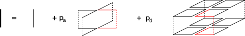
Figure 15: Example of smearing of a single link. Sum of orthogonal staples and diagonal staples are weighted with two independent parameters: $p_{a}$ and $p_{d}$. The figure is taken from [23].

The diagonal correlators of spatial Polyakov loops at different blocking levels are analysed using a single–state hyperbolic cosine fit to extract the effective mass, and jackknife bins are used to estimate the statistical errors. For all the points where we measure the string tension, the best projection onto the ground state is obtained at the maximum blocking level. This was confirmed using a variational procedure on the set of operators including all the different blocking levels. For example, in Fig. 16 we show the comparison between the mass extracted from diagonal correlators of the operator at the highest level of blocking and the one coming from the variational procedure. The comparison was done on a lattice with a longer temporal direction $L_{t}=2L_{4}$ and using the same fitting window for the effective mass plateaux in both cases.
On the points $(\beta_{4},\beta_{5},N_{4},N_{5})$ used for the measurements, we extracted the effective mass plateaux for the spatial Polyakov loops only at large temporal distances. The smearing and blocking algorithm allows for the extraction of a better signal, even though the parameters $(p_{a},p_{d})$ are not optimized for the broad range of lattice spacings $a_{4}$ explored in this work. In many cases, we still have small overlaps with the ground state, and consequently the single–state behaviour of the correlator can only be extracted at large temporal distances. An example of such cases is shown in Fig. 17(a), whereas in Fig. 17(b) we show one of the points where the plateaux is reached already at $t/a_{4}=2$.
A summary of all the torelon masses and their corresponding string tensions is reported in Tab. 6, and Tab. 8. The fitting range for the effective mass plateaux is also shown in the tables. Moreover, since the length of the Polyakov loops in lattice units is different between the $N_{5}=6$ lattices and the $N_{5}=4$ ones, we also report the physical size $L_{4}\sqrt{\sigma}$. As mentioned above, finite–size effects can be kept under control when $L_{4}\sqrt{\sigma}$ is large; in other words we would like our physical lattice volume to be much larger than the typical correlation length of the system, given by the inverse of the string tension.

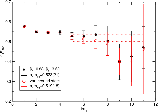
Figure 16: Comparison between the ground state effective mass extracted from the diagonal correlator of the highest blocking level (black points) and the one extracted from the variational procedure (red circles). The operators were $L_{4}=12a_{4}$ spatial Polyakov loops at $4$ different blocking levels, and their correlator was measured along a $L_{t}=2L_{4}=24a_{4}$ temporal distance. The correlator was averaged over the $N_{5}=6$ extra dimension slices.

(a)	(b)

Figure 17: Example of plateaux of torelon effective masses. (a) The final mass comes from a weighted fit of the points in the plateaux that is reached only at $t/a_{4}=3$ due to the small overlap of the operator onto the ground state. (b) At lower masses the plateaux is longer and the signal is extracted more reliably.

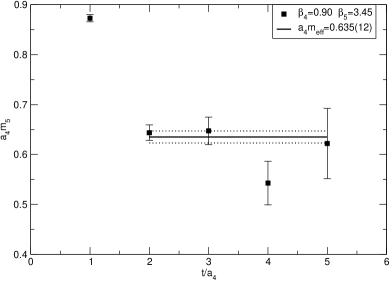
(a)	(b)

Figure 18: Example of plateaux for one of the highest scalar masses (a) and one of the lowest (b). (a) The operator overlaps poorly on the ground state and the plateaux is reached at large temporal distances. In this case we tried to estimate the systematic error on the fitting range, by choosing two different fitting windows. (b) The plateaux is reached already at $t/a_{4}=2$.

For the mass of the static scalar mode, we use compact Polyakov loop operators, that is gauge–invariant combinations of Polyakov loops winding around the extra fifth dimension. Such operators transform as scalars under the cubic symmetry group and they only carry a site index in the four–dimensional subspace. In particular, we choose two different combinations

$$\mathcal{O}_{1}(t)\;=\;\sum_{x}{\rm Tr}~{}[L_{5}(x,t)]\;;\qquad L_{5}(x,t)=\prod_{j=1}^{N_{5}}\mathcal{U}_{5}(x+ja_{5}\hat{5},t)\;,$$ (33)

and

$$\mathcal{O}_{2}(t)\;=\;\sum_{x}{\rm Tr}~{}[\phi(x,t)\phi^{\dagger}(x,t)]\;;\qquad\phi(x,t)=\frac{L_{5}-L_{5}^{\dagger}}{2}\;.$$ (34)

The sum $\sum_{x}$ is an average over the spatial volume in order to obtain zero–momentum operators on a fixed timeslice $t$. We average the correlators over the extra–dimensional coordinate, as in the previous case.
The first operator $\mathcal{O}_{1}$ is the same one used in Ref. [13]. For the operator in Eq. (34) it is possible to apply a smearing procedure following the one introduced in Ref. [24] for a scalar Higgs field. The operator $\phi$ is replaced by a smeared version that consists of a gauge–invariant combination of parallel transporters in the three–dimensional spatial subspace.
For this observable, we found the lowest smearing level of $\mathcal{O}_{2}$ to have the largest projection onto the ground state. The effective masses extracted from $\mathcal{O}_{1}$ and the lowest smearing level of $\mathcal{O}_{2}$ are always compatible. In some cases, usually at very low masses $a_{4}m_{5}$, the smeared operators show better plateaux, but we have not yet studied their projection onto the ground state with a more systematic variational procedure. At this stage we have not implemented more efficient noise–reduction techniques, such as a better choice for the smearing parameters, a multi–level algorithm [25], or a multi–hit procedure. As a consequence, we obtain plateaux like the ones shown in Fig. 18(a). The mass is extracted from a weighted fit of three, or sometimes even two, points at very large temporal distance, where the signal–to–noise ratio is quite small. Clearly there also points where the scalar mass is small, and the effective mass plateaux is well behaved. An example can be found in Fig. 18(b). We summarize the scalar masses $a_{4}m_{5}$, and the fitting windows for the plateaux in Tab. 5, and Tab. 7.

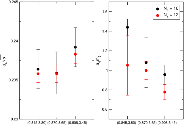
Figure 19: For three different points reported on the $x$ axis, we show the string tension and the scalar mass in units of the cut–off length. Two volumes are compared and sizable finite–size effects can be ruled out.

An attempt to estimate the finite–volume effects on the observables $a_{4}\sqrt{\sigma}$ and $a_{4}m_{5}$ has been performed at $N_{5}=6$. For three different points in the phase space $(\beta_{4},\beta_{5})$, we simulate two different four–dimensional lattice sizes, $N_{4}=12$ and $N_{4}=16$. The three points have a very similar string tension at $N_{4}=12$, but on that volume $L_{4}\sqrt{\sigma}$ turns out to be smaller than $3$. The results are summarized in Tab. 2. The string tension and the scalar mass are not affected by the change of four–dimensional volume. In Fig. 19 the volume dependence is shown for both the observables. The larger statistical error for $a_{4}\sqrt{\sigma}$ on the largest volume is due to the larger torelon mass at $N_{4}=16$ (the number of configurations is the same for both volumes).

	$a_{4}\sqrt{\sigma}$		$a_{4}m_{5}$
$N_{4}$	12	16	12	16
(0.845,3.80)	0.2358(11)	0.2364(25)	1.05(31)	1.44(9)
(0.870,3.65)	0.2358(11)	0.2359(27)	0.998(93)	1.08(26)
(0.870,3.65)	0.2383(12)	0.2392(25)	0.777(78)	0.956(99)

Table 2: Comparison between the observables on two different four–dimensional volumes and fixed $N_{5}=6$. The string tensions are independent of $N_{4}$ and the scalar masses are compatible within one standard deviation.

Mixing with scalar glueball states

Since we are studying a strongly coupled Yang–Mills theory, the low–energy dynamics could be affected by the presence of non–perturbative states, such as glueballs. It is well known that the lightest glueball state appears in the scalar channel. However, this is the same symmetry channel where we perturbatively expect to see a light particle due to the compactification mechanism. It is therefore mandatory to check whether these two states mix in order to shed light on the non–perturbative fate of Eq. (1).
Lattice calculations of glueball masses suffer from the aforementioned problems in relation to torelon masses: to obtain an accurate estimate of the mass from correlation functions, one needs to adopt noise–reduction techniques. We used a combination of the improved diagonal smearing described in Fig. 15 and a variational ansatz. We used three different spatially shaped Wilson loops in order to construct glueball operators. This procedure has been very succesfull in extracting highly accurate glueball masses in three and four–dimensional ${\rm SU(}N{\rm)}$ gauge theories [22, 23, 26].
To create operators coupling to glueball states in four dimensions, we use the four–links plaquette, the six–links rectangular plaquette and the six–links chair shown in Fig. 20. Symmetrized combinations of these operators projecting only onto the scalar representation of the three–dimensional cubic symmetry group are then correlated together with operators in Eq. (33) and Eq. (34); we refer to these scalar glueball operators as $\mathcal{O}_{a}$, $\mathcal{O}_{b}$ and $\mathcal{O}_{c}$ built starting respectively from the path a), b) and c) in Fig. 20 (we always use zero–momentum projections).

Figure 20: Wilson loops used in the construction of glueball operators in the scalar channel. Each of these three operators is smeared according to Fig. 15 in order to construct a larger variational ansatz.

We expect that the operators in Fig. 20 will couple mainly onto glueball states as they are built entirely from links in the three–dimensional spatial subspace of the lattice. On the other hand, we suggest that the operators in Eq. (33) and Eq. (34) will couple mainly with states of extra–dimensional nature because they are built from links in the extra direction. Inevitably, due to the non–perturbative nature of the theory, the masses of the scalar state extracted from correlators of the latter type of operators could be affected by non–negligible mixing with glueball states. We studied the contribution of this mixing, and the results are reported and explained in Sec. 5.
To estimate the mixing in the scalar spectrum of the lattice theory, we used the following procedure:

• compute the full correlation matrix $C_{\alpha\beta}(t)$, where the lower indices run over the scalar operators of the following type: $\mathcal{O}_{2}$, $\mathcal{O}_{a}$, $\mathcal{O}_{b}$, $\mathcal{O}_{c}$

• employ a variational procedure to find a linear combination of the correlated operators such that the propagating state is the lightest (or apply the procedure on the orthogonal space to get the excited ones)

• decompose the approximate mass eigenstates obtained from the previous step into their projections onto the basis operators $\mathcal{O}_{2}$, $\mathcal{O}_{a}$, $\mathcal{O}_{b}$, $\mathcal{O}_{c}$.

The last step of this variational analysis gives us informations about the nature of the propagating state. If the main projection is onto glueball operators $\mathcal{O}_{a}$, $\mathcal{O}_{b}$ and $\mathcal{O}_{c}$, the mass extracted is likely to be associated to a glueball state rather than a scalar of extra–dimensional origin. At the same time, a projection onto $\mathcal{O}_{2}$ of more than $50\%$ indicates that the state investigated is probably a scalar coming from the compactification mechanism.
Due to the large computational cost, we measured the full correlation matrix $C_{\alpha\beta}(t)$ only on a subset of the points reported in Tab. 3: we choose points at fixed $\gamma\approx 1.54$ and we investigate how the mixing of the extracted states changes as we increase $\beta$, moving away from the line of second order phase transition. On these points, the masses extracted using only correlators of $\mathcal{O}_{1}$ and $\mathcal{O}_{2}$, as described in the previous section, has been shown in Fig. 8. In order to extract a more reliable plateau, we increased the number of lattice points in the temporal direction $L_{t}=2L_{4}$; this allowed us to follow the plateaux of the effective mass for a wider range of temporal distances, usually corresponding to a fitting range $t_{\rm min}-t_{\rm max}=[3-7]$ in units of the lattice spacing $a_{4}$ (cfr. for example the fitting ranges of Tab. 5). The results for the spectrum of the theory in the scalar channel at $\gamma\approx 1.54$ is summarized in Fig. 8. An example of the effective mass plateax for the ground state and its low–energy excitations is also shown in Fig. 21 for two values of $\beta$; we compare the results of the variational procedure, with the results obtained from diagonal correlators of pure scalar operators.

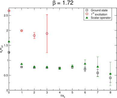
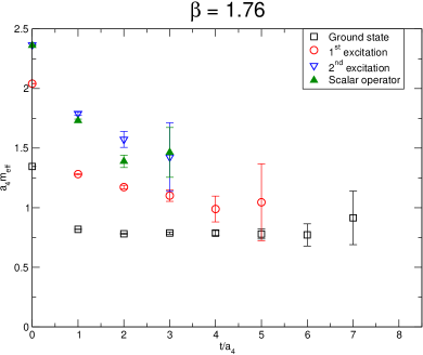
(a)	(b)

Figure 21: Example of effective mass plateaux for two different values of $\beta$. (a) At $\beta=1.72$ the mass of the low–lying scalar state obtained from the variational ansatz is compatible with the one we measured using only scalar operators. (b) At $\beta=1.76$ the scalar operator yelds a mass which is compatible with the second excitations of the scalar spectrum.

In the range of parameters explored with the full variational ansatz, we notice that the relative mixing of the scalar states in the spectrum with the different operators in the correlator matrix changes with $\beta$. The mixing of the extracted ground state is shown in Fig. 9. The relative projections for both sets of operators are shown for different values of $\beta$. The plot clearly shows the contribution of the operator $\mathcal{O}_{2}$ to the ground state of the scalar channel decreasing as $\beta$ increases. We recall here that increasing $\beta$ at fixed anisotropy corresponds to going towards the weak–coupling limit. This is the same limit taken in the simulations of Ref. [13], where it has been shown how the mass extracted from correlators of our $\mathcal{O}_{1}$ diverges and decouples from the low–energy spectrum. It is therefore not surprising that the lightest glueballs become relevant to the dynamics of the theory in this region of the parameter space. On the other hand, we clearly see that at lower values of $\beta$, closer to the line of second order phase transition, the scalar state has a dominant contribution from the extra–dimensional operator $\mathcal{O}_{2}$ and it increases as we lower the values of $\beta$.
Another interesting mixing we looked at is shown in Fig. 10. The plots show the relative mixing of the first excited state onto the operators in the variational set. The points where the mixing is calculated are the same as in Fig. 9. Up to $\beta=1.75$, the first excited state is dominated by a projection onto the scalar operator $\mathcal{O}_{2}$, suggesting an extra–dimensional nature for this particle. What it is not shown is that at $\beta=1.76$, we find the second excited state to project mostly onto $\mathcal{O}_{2}$ (cfr. Fig.21(b)).

$N_{4}=10$ $N_{5}=4$
$\beta_{4}$	$\beta_{5}$	$\beta$	$\gamma$	$\frac{N_{5}}{\gamma}$	$\xi$	$\frac{N_{5}}{\xi}$
1.00	2.90	1.7029	1.7029	2.3488	2.291(39)	1.744(29)
1.00	3.00	1.7320	1.7320	2.3094	2.339(40)	1.709(29)
1.05	2.65	1.6680	1.5886	2.5178	2.095(39)	1.911(35)
1.05	2.70	1.6837	1.6035	2.4944	2.119(38)	1.889(35)
1.05	2.80	1.7146	1.6329	2.4494	2.169(36)	1.844(32)
1.05	2.90	1.7449	1.6619	2.4068	2.219(37)	1.801(31)
1.05	3.00	1.7748	1.6903	2.3664	2.268(38)	1.764(30)
1.07	2.65	1.6838	1.5737	2.5417	2.067(43)	1.934(37)
1.07	2.70	1.6997	1.5885	2.5180	2.092(40)	1.911(35)
1.07	2.75	1.7153	1.6031	2.4950	2.117(40)	1.889(34)
1.07	2.80	1.7309	1.6176	2.4727	2.141(38)	1.866(33)
1.07	2.90	1.7615	1.6462	2.4297	2.195(38)	1.824(30)
1.09	2.65	1.6995	1.5592	2.5653	2.040(43)	1.959(39)
1.09	2.70	1.7155	1.5738	2.5415	2.068(41)	1.934(38)
1.10	2.65	1.7073	1.5521	2.5771	2.029(42)	1.969(41)
1.10	2.70	1.7233	1.5667	2.5531	2.056(41)	1.948(39)
1.10	2.80	1.7549	1.5954	2.5071	2.105(38)	1.900(36)
1.10	2.90	1.7860	1.6236	2.4635	2.152(37)	1.858(33)
1.10	3.00	1.8165	1.6514	2.4221	2.202(38)	1.815(32)
1.11	2.65	1.7150	1.5451	2.5888	2.018(44)	1.986(43)
1.11	2.70	1.7311	1.5596	2.5647	2.042(42)	1.959(41)
1.12	2.65	1.7227	1.5382	2.6004	2.009(44)	1.998(44)
1.12	2.70	1.7389	1.5526	2.5762	2.032(42)	1.972(43)
1.13	2.65	1.7304	1.5313	2.6120	1.995(45)	2.008(47)
1.13	2.70	1.7467	1.5457	2.5877	2.019(44)	1.984(45)
1.14	2.65	1.7381	1.5246	2.6235	1.981(45)	2.019(45)
1.14	2.70	1.7544	1.5389	2.5991	2.007(45)	1.995(44)
1.15	2.60	1.7291	1.5036	2.6602	1.944(47)	2.059(58)
1.15	2.65	1.7457	1.5180	2.6350	1.969(45)	2.031(48)
1.15	2.70	1.7621	1.5322	2.6105	1.996(43)	2.006(45)
1.15	2.80	1.7944	1.5603	2.5634	2.043(40)	1.955(40)
1.15	2.90	1.8262	1.588	2.5188	2.092(37)	1.912(36)
1.15	3.00	1.8574	1.6151	2.4765	2.139(38)	1.869(34)
1.20	2.50	1.7320	1.4433	2.7712	1.839(50)	2.180(58)
1.20	2.55	1.7492	1.4577	2.7439	1.861(49)	2.151(58)
1.20	2.60	1.7663	1.4719	2.7174	1.886(50)	2.121(54)
1.20	2.65	1.7832	1.4860	2.6917	1.912(48)	2.091(51)
1.20	2.70	1.8000	1.5000	2.6666	1.939(49)	2.063(53)
1.10153	2.62363	1.70	1.54	2.59	2.014(44)	1.986(42)
1.10801	2.63906	1.71	1.54	2.59	2.014(44)	1.986(42)
1.11449	2.6545	1.72	1.54	2.59	2.014(44)	1.986(42)
1.12097	2.66993	1.73	1.54	2.59	2.014(44)	1.986(42)
1.12745	2.68536	1.74	1.54	2.59	2.014(44)	1.986(42)
1.13393	2.70079	1.75	1.54	2.59	2.014(44)	1.986(42)
1.14041	2.71623	1.76	1.54	2.59	2.014(44)	1.986(42)
1.14688	2.73166	1.77	1.54	2.59	2.014(44)	1.986(42)

Table 3: This table give the details of the simulated points on the $10^{4}\times 4$ lattice. Together with the bare parameters $\beta_{4}$, $\beta_{5}$, $\beta$, $\gamma$ and $\frac{N_{5}}{\gamma}$, we report the values of the renormalised anisotropy $\xi$ from the interpolation shown in Fig. 5, and the corresponding scale separation $\frac{\Lambda_{\rm UV}}{\Lambda_{\rm R}}=\frac{N_{5}}{\xi}$.

$N_{4}=12$ $N_{5}=6$
$\beta_{4}$	$\beta_{5}$	$\beta$	$\gamma$	$\frac{N_{5}}{\gamma}$	$\xi$	$\frac{N_{5}}{\xi}$
0.845	3.80	1.7919	2.1206	2.8293	2.976(30)	2.016(19)
0.850	3.75	1.7853	2.1004	2.8565	2.941(30)	2.039(20)
0.850	3.85	1.8090	2.1282	2.8192	2.988(31)	2.008(20)
0.855	3.70	1.7786	2.0802	2.8842	2.909(27)	2.061(20)
0.855	3.75	1.7906	2.0942	2.8649	2.934(29)	2.045(19)
0.855	3.80	1.8025	2.1081	2.8460	2.957(29)	2.029(20)
0.855	3.85	1.8143	2.1220	2.8275	2.978(31)	2.016(20)
0.860	3.70	1.7838	2.0742	2.8926	2.902(29)	2.069(20)
0.860	3.75	1.7958	2.0881	2.8733	2.923(29)	2.053(20)
0.860	3.80	1.8077	2.1020	2.8543	2.945(28)	2.038(20)
0.860	3.85	1.8196	2.1158	2.8357	2.968(29)	2.022(20)
0.865	3.55	1.7523	2.0258	2.9617	2.823(32)	2.126(23)
0.865	3.60	1.7646	2.0400	2.9410	2.846(31)	2.109(23)
0.865	3.65	1.7768	2.0541	2.9208	2.869(29)	2.092(21)
0.865	3.70	1.7889	2.0682	2.9010	2.889(29)	2.076(21)
0.865	3.80	1.8130	2.0959	2.8626	2.936(30)	2.045(21)
0.870	3.55	1.7574	2.0200	2.9702	2.811(32)	2.133(24)
0.870	3.60	1.7697	2.0341	2.9495	2.836(32)	2.117(23)
0.870	3.65	1.7819	2.0482	2.9293	2.858(30)	2.099(23)
0.870	3.70	1.7941	2.0622	2.9094	2.880(29)	2.083(22)
0.875	3.55	1.7624	2.0142	2.9788	2.802(33)	2.140(24)
0.875	3.60	1.7748	2.0283	2.9580	2.823(31)	2.123(24)
0.875	3.65	1.7871	2.0424	2.9377	2.849(31)	2.106(22)
0.875	3.70	1.7993	2.0563	2.9177	2.872(29)	2.090(21)
0.880	3.55	1.7674	2.0085	2.9873	2.792(34)	2.149(25)
0.888	3.50	1.7629	1.9853	3.0222	2.755(34)	2.179(26)
0.890	3.55	1.7775	1.9971	3.0042	2.775(35)	2.163(27)
0.900	3.45	1.7621	1.9578	3.0645	2.711(31)	2.212(26)
0.900	3.50	1.7748	1.9720	3.0425	2.735(32)	2.194(27)
0.900	3.55	1.7874	1.9860	3.0210	2.756(33)	2.178(26)
0.908	3.45	1.7699	1.9492	3.0781	2.699(33)	2.226(25)
0.920	3.40	1.7686	1.9224	3.1210	2.653(31)	2.261(26)
0.920	3.45	1.7815	1.9364	3.0983	2.676(32)	2.241(26)
0.920	3.50	1.7944	1.9504	3.0761	2.699(30)	2.223(26)
0.860	3.60	1.7595	2.0459	2.9325	2.855(30)	2.102(22)
0.880	3.60	1.7798	2.0226	2.9664	2.816(33)	2.131(25)
0.900	3.60	1.8000	2.0000	3.0000	2.777(34)	2.159(26)
0.920	3.55	1.8072	1.9643	3.0544	2.722(33)	2.205(26)
0.920	3.60	1.8198	1.9781	3.0331	2.743(32)	2.187(27)
0.940	3.40	1.7877	1.9018	3.1548	2.619(30)	2.291(26)
0.940	3.50	1.8138	1.9296	3.1094	2.665(30)	2.251(26)
0.940	3.60	1.8395	1.9569	3.0659	2.709(31)	2.215(25)

Table 4: This table give the details of the simulated points on the $12^{4}\times 6$ lattice. Together with the bare parameters $\beta_{4}$, $\beta_{5}$, $\beta$, $\gamma$ and $\frac{N_{5}}{\gamma}$, we report the values of the renormalised anisotropy $\xi$ from the interpolation shown in Fig. 5, and the corresponding scale separation $\frac{\Lambda_{\rm UV}}{\Lambda_{\rm R}}=\frac{N_{5}}{\xi}$.

Scalar masses on $N_{4}=10$ $N_{5}=4$
$\beta_{4}$	$\beta_{5}$	$a_{4}m_{5}$	$t_{\rm min}-t_{\rm max}$
1.00	2.90	1.118(26)	2 - 4
1.00	3.00	1.406(56)	2 - 4
1.00	3.00	1.30(19)	3 - 4
1.05	2.80	1.020(16)	2 - 4
1.05	3.00	1.386(85)	2 - 4
1.05	3.00	1.05(22)	3 - 4
1.07	2.70	0.6482(69)	2 - 4
1.07	2.75	0.925(13)	2 - 4
1.07	2.75	0.904(29)	3 - 4
1.07	2.80	1.022(57)	3 - 4
1.07	2.90	1.349(56)	2 - 4
1.07	2.90	1.27(21)	3 - 4
1.09	2.65	0.4586(43)	2 - 4
1.09	2.70	0.844(10)	2 - 4
1.10	2.65	0.624(05)	2 - 4
1.10	2.70	0.880(14)	2 - 4
1.10	2.80	1.258(51)	2 - 4
1.10	2.80	1.15(15)	3 - 4
1.10	2.90	1.64(17)	2 - 4
1.11	2.65	0.732(11)	2 - 4
1.11	2.70	0.865(32)	3 - 4
1.12	2.65	0.779(11)	2 - 4
1.14	2.65	0.840(52)	3 - 4
1.14	2.70	0.90(13)	3 - 4
1.15	2.60	0.724(21)	3 - 4
1.15	2.70	1.424(55)	2 - 4
1.15	2.70	1.24(21)	3 - 4
1.20	2.50	0.923(76)	3 - 4
1.10801	2.63906	0.638(44)	3 - 4
1.11449	2.6545	0.765(12)	3 - 4
1.12097	2.66993	0.822(26)	3 - 4
1.12745	2.68536	0.898(37)	3 - 4
1.13393	2.70079	0.791(98)	3 - 4
1.14041	2.71623	1.450(92)	2 - 4
1.14041	2.71623	1.18(34)	3 - 4

Table 5: Measured scalar masses on the $10^{4}\times 4$ lattice. The fitting range for the effective mass plateaux is shown in the last column. Boldface values are alternative fitting ranges.

Torelon masses and string tensions on $N_{4}=10$ $N_{5}=4$
$\beta_{4}$	$\beta_{5}$	$a_{4}m_{\rm tor}$	$t_{\rm min}-t_{\rm max}$	$a_{4}\sqrt{\sigma}$	$\sim L_{4}\sqrt{\sigma}$
1.05	3.00	1.219(24)	2 - 4	0.3638(33)	3.6
1.05	3.00	1.173(71)	3 - 4	0.3574(99)	3.6
1.07	2.90	1.334(39)	2 - 4	0.3793(52)	3.8
1.07	2.90	1.16(11)	3 - 4	0.356(15)	3.6
1.10	2.80	1.116(16)	2 - 4	0.3493(23)	3.5
1.10	2.80	1.105(48)	3 - 4	0.3478(69)	3.5
1.10	2.90	0.428(2)	2 - 4	0.2308(5)	2.3
1.14	2.65	1.215(27)	2 - 4	0.3633(37)	3.6
1.14	2.65	1.190(71)	3 - 4	0.3598(99)	3.6
1.14	2.70	0.6153(39)	2 - 4	0.2683(7)	2.7
1.15	2.70	0.3798(14)	2 - 4	0.2201(3)	2.2
1.20	2.50	0.5663(41)	2 - 4	0.2590(8)	2.6
1.12745	2.68536	1.18(10)	3 - 4	0.358(14)	3.6
1.13393	2.70079	0.8175(78)	2 - 4	0.3037(13)	3.0
1.14041	2.71623	0.491(3)	2 - 3	0.2441(6)	2.4

Table 6: Measured torelon masses on the $10^{4}\times 4$ lattice. The fitting range for the effective mass plateaux is shown together with the calculated string tension. Boldface values are alternative fitting ranges. The last column states the spatial length of the lattice in units of the four dimensional correlation length given by the inverse of the string tension.

Scalar masses on $N_{4}=12$ $N_{5}=6$
$\beta_{4}$	$\beta_{5}$	$a_{4}m_{5}$	$t_{\rm min}-t_{\rm max}$
0.845	3.80	1.05(31)	3 - 5
0.845	3.80	1.17(20)	3 - 5
0.850	3.75	1.273(74)	2 - 3
0.850	3.75	1.14(19)	3 - 4
0.850	3.85	1.65(15)	2 - 4
0.850	3.85	1.04(36)	3 - 4
0.855	3.70	0.91(14)	3 - 5
0.855	3.75	1.35(25)	3 - 5
0.860	3.60	0.581(20)	4 - 7
0.860	3.70	1.294(67)	2 - 4
0.860	3.70	1.19(24)	3 - 4
0.865	3.55	0.3312(38)	2 - 4
0.865	3.60	0.677(25)	4 - 5
0.865	3.65	0.95(10)	3 - 5
0.870	3.55	0.4679(86)	4 - 5
0.870	3.60	0.818(58)	3 - 4
0.870	3.65	0.998(93)	3 - 5
0.870	3.70	1.401(92)	2 - 4
0.870	3.70	1.07(26)	3 - 4
0.875	3.55	0.532(20)	4 - 5
0.875	3.60	0.880(97)	3 - 4
0.875	3.65	1.40(8)	2 - 4
0.875	3.65	1.16(25)	3 - 4
0.875	3.70	1.02(20)	3 - 5
0.880	3.55	0.727(50)	3 - 5
0.880	3.55	0.86(15)	3 - 5
0.880	3.60	1.318(57)	2 - 4
0.880	3.60	1.30(21)	3 - 4
0.888	3.50	0.595(19)	3 - 5
0.888	3.50	0.561(34)	4 - 5
0.890	3.55	1.038(82)	3 - 5
0.890	3.55	0.93(21)	4 - 5
0.900	3.45	0.635(12)	2 - 5
0.900	3.50	1.173(72)	2 - 5
0.900	3.50	0.91(13)	4 - 5
0.908	3.45	0.777(78)	3 - 5
0.920	3.45	1.46(11)	2 - 4
0.920	3.45	1.06(33)	3 - 4

Table 7: Measured scalar masses on the $12^{4}\times 6$ lattice. The fitting range for the effective mass plateaux is shown in the last column. Boldface values are alternative fitting ranges. Boldface masses come from a different choice of the scalar operator in the correlator. (The starred points come from a lattice with a longer temporal distance $L_{t}=2L_{4}$)

Torelon masses and string tensions on $N_{4}=12$ $N_{5}=6$
$\beta_{4}$	$\beta_{5}$	$a_{4}m_{\rm tor}$	$t_{\rm min}-t_{\rm max}$	$a_{4}\sqrt{\sigma}$	$\sim L_{4}\sqrt{\sigma}$
0.845	3.80	0.5800(60)	2 - 5	0.2358(11)	2.8
0.850	3.75	0.7127(75)	2 - 5	0.2582(12)	3.1
0.850	3.75	0.730(16)	3 - 5	0.2610(26)	3.1
0.850	3.85	0.2665(19)	2 - 4	0.1717(4)	2.1
0.850	3.85	0.2658(18)	3 - 4	0.1715(4)	2.1
0.855	3.70	0.8954(99)	2 - 5	0.2862(14)	3.4
0.855	3.75	0.5162(51)	2 - 5	0.2243(9)	2.7
0.860	3.70	0.6412(73)	2 - 5	0.2464(12)	3.0
0.865	3.65	0.808(19)	3 - 5	0.2732(29)	3.3
0.865	3.65	0.784(34)	4 - 5	0.2694(53)	3.2
0.870	3.60	1.224(77)	3 - 5	0.3306(97)	4.0
0.870	3.65	0.5798(62)	2 - 5	0.2358(11)	2.8
0.870	3.70	0.3295(19)	2 - 5	0.1864(4)	2.2
0.875	3.60	0.7933(92)	2 - 4	0.2709(14)	3.3
0.875	3.65	0.4177(31)	2 - 5	0.2051(6)	2.5
0.875	3.70	0.2418(10)	3 - 5	0.1656(2)	2.0
0.880	3.55	1.25(12)	3 - 5	0.334(14)	4.0
0.880	3.60	0.523(21)	5 - 11	0.2256(40)	2.7
0.890	3.55	0.5140(49)	2 - 5	0.2239(9)	2.7
0.900	3.45	1.06(11)	3 - 5	0.310(15)	3.7
0.900	3.45	0.87(25)	4 - 5	0.282(37)	3.4
0.900	3.50	0.4963(52)	2 - 5	0.2205(10)	2.6
0.908	3.45	0.5942(67)	2 - 5	0.2383(12)	2.9
0.920	3.45	0.2353(19)	2 - 4	0.1639(5)	2.0

Table 8: Measured torelon masses on the $12^{4}\times 6$ lattice. The fitting range for the effective mass plateaux is shown together with the calculated string tension. Boldface values are alternative fitting ranges. The last column states the spatial length of the lattice in units of the four dimensional correlation length given by the inverse of the string tension. (The starred point comes from a lattice with a longer temporal distance $L_{t}=2L_{4}$)

$N_{4}=10$ $N_{5}=4$
$\frac{\Lambda_{\rm UV}}{\Lambda_{\rm R}}$	$a_{4}\sqrt{\sigma}$	$R\sqrt{\sigma}$	$\frac{m_{5}}{\sqrt{\sigma}}$	$Rm_{5}$
1.763(29)	0.3638(33)	0.1021(19)	3.81(23)	0.389(25)
1.763(29)	0.3638(33)	0.1021(19)	2.89(61)	0.295(63)
1.763(29)	0.3574(99)	0.1003(32)	3.88(26)	0.389(29)
1.763(29)	0.3574(99)	0.1003(32)	2.95(62)	0.295(63)
1.824(30)	0.3793(52)	0.1101(23)	3.56(15)	0.392(19)
1.824(30)	0.3793(52)	0.1101(23)	3.35(54)	0.369(60)
1.824(30)	0.356(15)	0.1033(48)	3.79(21)	0.392(28)
1.824(30)	0.356(15)	0.1033(48)	3.57(57)	0.369(62)
1.900(35)	0.3493(23)	0.1056(21)	3.60(14)	0.380(17)
1.900(35)	0.3493(23)	0.1056(21)	3.29(41)	0.348(44)
1.900(35)	0.3478(69)	0.1052(29)	3.62(16)	0.380(20)
1.900(35)	0.3478(69)	0.1052(29)	3.31(41)	0.348(44)
1.857(32)	0.2308(5)	0.0682(12)	7.10(75)	0.484(52)
2.019(45)	0.3633(37)	0.1168(29)	2.31(15)	0.270(18)
2.019(45)	0.3598(99)	0.1156(41)	2.33(16)	0.270(20)
1.994(43)	0.2683(7)	0.0852(19)	3.36(50)	0.286(43)
2.006(44)	0.2201(33)	0.0703(15)	6.47(24)	0.455(20)
2.006(44)	0.2201(33)	0.0703(15)	5.66(94)	0.397(67)
2.180(57)	0.2590(8)	0.0899(24)	3.56(30)	0.320(28)
1.986(42)	0.358(14)	0.1133(51)	2.51(14)	0.284(20)
1.986(42)	0.3037(13)	0.0960(21)	2.61(32)	0.250(31)
1.986(42)	0.2441(6)	0.0772(16)	5.94(38)	0.458(31)
1.986(42)	0.2441(6)	0.0772(16)	4.9(1.4)	0.37(11)

Table 9: The results of our numerical simulations are reported in this table for $N_{5}=4$. The primary observables directly measured in the simulations, $a_{4}\sqrt{\sigma}$ and $a_{4}m_{5}$, are used to obtain the combinations $\frac{m_{5}}{\sqrt{\sigma}}$, $R\sqrt{\sigma}$ and $Rm_{5}$. This is done using the value for the separation of the cut–off scale from the compactification scale $\frac{\Lambda_{\rm UV}}{\Lambda_{\rm R}}$. When more than one value is shown, they come from different fitting ranges in the plateaux of the primary observables. The spread of the values is used to estimate a systematic error that is then reported in the plots.

$N_{4}=12$ $N_{5}=6$
$\frac{\Lambda_{\rm UV}}{\Lambda_{\rm R}}$	$a_{4}\sqrt{\sigma}$	$R\sqrt{\sigma}$	$\frac{m_{5}}{\sqrt{\sigma}}$	$Rm_{5}$
2.016(19)	0.2358(11)	0.0757(8)	4.5(1.3)	0.337(99)
2.016(19)	0.2358(11)	0.0757(8)	4.98(84)	0.377(64)
2.039(20)	0.2582(12)	0.0838(9)	4.93(29)	0.413(25)
2.039(20)	0.2610(26)	0.0847(12)	4.88(29)	0.413(25)
2.039(20)	0.2582(12)	0.0838(9)	4.41(75)	0.369(63)
2.039(20)	0.2610(26)	0.0847(12)	4.36(74)	0.369(63)
2.008(20)	0.1717(5)	0.0549(6)	9.59(88)	0.526(49)
2.008(20)	0.1715(4)	0.0548(6)	9.60(88)	0.526(49)
2.008(20)	0.1717(5)	0.0549(6)	6.1(2.1)	0.33(12)
2.008(20)	0.1715(4)	0.0548(6)	6.1(2.1)	0.33(12)
2.061(19)	0.2862(14)	0.0939(10)	3.20(48)	0.300(45)
2.045(19)	0.2243(9)	0.0730(8)	6.0(1.1)	0.439(80)
2.069(20)	0.2464(12)	0.0811(9)	5.25(28)	0.426(23)
2.069(20)	0.2464(12)	0.0811(9)	4.84(98)	0.393(79)
2.092(21)	0.2732(29)	0.0910(13)	3.49(38)	0.317(35)
2.092(21)	0.2694(53)	0.0897(20)	3.54(39)	0.317(35)
2.117(23)	0.3306(97)	0.1114(35)	2.47(19)	0.276(23)
2.099(23)	0.2358(11)	0.0788(9)	4.23(39)	0.333(31)
2.083(22)	0.1864(41)	0.0618(7)	7.52(50)	0.464(31)
2.083(22)	0.1864(41)	0.0618(7)	5.7(1.4)	0.355(86)
2.123(24)	0.2709(14)	0.0915(11)	3.25(36)	0.297(33)
2.106(22)	0.2051(64)	0.0688(7)	6.83(41)	0.469(29)
2.106(22)	0.2051(64)	0.0688(7)	5.6(1.2)	0.388(84)
2.090(21)	0.1656(2)	0.0551(5)	6.2(1.2)	0.339(65)
2.149(25)	0.334(14)	0.1144(51)	2.18(18)	0.249(24)
2.149(25)	0.334(14)	0.1144(51)	2.57(45)	0.294(53)
2.131(25)	0.2256(40)	0.0765(16)	5.84(25)	0.447(21)
2.131(25)	0.2256(40)	0.0765(16)	5.76(92)	0.441(71)
2.163(27)	0.2239(9)	0.0771(10)	4.64(37)	0.357(29)
2.163(27)	0.2239(9)	0.0771(10)	4.16(93)	0.320(72)
2.212(26)	0.310(15)	0.1090(54)	2.05(11)	0.224(16)
2.212(26)	0.282(37)	0.099(13)	2.25(31)	0.224(42)
2.194(27)	0.2205(10)	0.0770(10)	5.32(33)	0.410(26)
2.194(27)	0.2205(10)	0.0770(10)	4.12(60)	0.317(46)
2.226(25)	0.2383(12)	0.0844(10)	3.26(33)	0.275(28)
2.241(26)	0.1639(5)	0.0585(69)	8.90(66)	0.520(39)
2.241(26)	0.1639(5)	0.0585(69)	6.4(2.0)	0.38(12)

Table 10: The results of our numerical simulations are reported in this table for $N_{5}=6$. The primary observables directly measured in the simulations, $a_{4}\sqrt{\sigma}$ and $a_{4}m_{5}$, are used to obtain the combinations $\frac{m_{5}}{\sqrt{\sigma}}$, $R\sqrt{\sigma}$ and $Rm_{5}$. This is done using the value for the separation of the cut–off scale from the compactification scale $\frac{\Lambda_{\rm UV}}{\Lambda_{\rm R}}$. When more than one value is shown, they come from different fitting ranges in the plateaux of the primary observables. The spread of the values is used to estimate a systematic error that is then reported in the plots.

References

- [1] T. Kaluza, On the Problem of Unity in Physics, Sitzungsber.Preuss.Akad.Wiss.Berlin (Math.Phys.) 1921 (1921) 966–972.
- [2] O. Klein, Quantum Theory and Five-Dimensional Theory of Relativity. (In German and English), Z.Phys. 37 (1926) 895–906.
- [3] Y. Hosotani, Dynamical Mass Generation by Compact Extra Dimensions, Phys. Lett. B126 (1983) 309.
- [4] H. Hatanaka, T. Inami, and C. S. Lim, The gauge hierarchy problem and higher dimensional gauge theories, Mod. Phys. Lett. A13 (1998) 2601–2612, [hep-th/9805067].
- [5] H.-C. Cheng, K. T. Matchev, and M. Schmaltz, Radiative corrections to Kaluza-Klein masses, Phys. Rev. D66 (2002) 036005, [hep-ph/0204342].
- [6] G. von Gersdorff, N. Irges, and M. Quiros, Bulk and brane radiative effects in gauge theories on orbifolds, Nucl. Phys. B635 (2002) 127–157, [hep-th/0204223].
- [7] Y. Hosotani, Dynamical gauge symmetry breaking by Wilson lines in the electroweak theory, hep-ph/0504272.
- [8] Y. Hosotani, N. Maru, K. Takenaga, and T. Yamashita, Two loop finiteness of Higgs mass and potential in the gauge-Higgs unification, Prog. Theor. Phys. 118 (2007) 1053–1068, [arXiv:0709.2844].
- [9] L. Del Debbio, E. Kerrane, and R. Russo, Mass corrections in string theory and lattice field theory, Phys. Rev. D80 (2009) 025003, [arXiv:0812.3129].
- [10] I. Antoniadis, A Possible new dimension at a few TeV, Phys.Lett. B246 (1990) 377–384.
- [11] S. Ejiri, J. Kubo, and M. Murata, A study on the nonperturbative existence of Yang-Mills theories with large extra dimensions, Phys. Rev. D62 (2000) 105025, [hep-ph/0006217].
- [12] S. Ejiri, S. Fujimoto, and J. Kubo, Scaling laws and effective dimension in lattice SU(2) Yang-Mills theory with a compactified extra dimension, Phys.Rev. D66 (2002) 036002, [hep-lat/0204022].
- [13] P. de Forcrand, A. Kurkela, and M. Panero, The phase diagram of Yang-Mills theory with a compact extra dimension, JHEP 06 (2010) 050, [arXiv:1003.4643].
- [14] F. Knechtli, M. Luz, and A. Rago, On the phase structure of five-dimensional SU(2) gauge theories with anisotropic couplings, Nucl.Phys. B856 (2012) 74–94, [arXiv:1110.4210].
- [15] K. Farakos and S. Vrentzos, Exploration of the phase diagram of 5d anisotropic SU(2) gauge theory, arXiv:1007.4442.
- [16] M. Creutz, Confinement and the Critical Dimensionality of Space- Time, Phys. Rev. Lett. 43 (1979) 553–556.
- [17] A. Hart and O. Philipsen, The spectrum of the three-dimensional adjoint Higgs model and hot SU(2) gauge theory, Nucl. Phys. B572 (2000) 243–265, [hep-lat/9908041].
- [18] A. Kurkela, P. de Forcrand, and M. Panero, Dimensional reduction and the phase diagram of 5d Yang-Mills theory, PoS LAT2009 (2009) 050, [arXiv:0911.3609].
- [19] S. Datta and S. Gupta, Dimensional reduction and screening masses in pure gauge theories at finite temperature, Nucl. Phys. B534 (1998) 392–416, [hep-lat/9806034].
- [20] S. Chandrasekharan and U. J. Wiese, Quantum link models: A discrete approach to gauge theories, Nucl. Phys. B492 (1997) 455–474, [hep-lat/9609042].
- [21] R. Brower, S. Chandrasekharan, and U. Wiese, QCD as a quantum link model, Phys.Rev. D60 (1999) 094502, [hep-th/9704106].
- [22] B. Lucini, M. Teper, and U. Wenger, Glueballs and k-strings in SU(N) gauge theories: Calculations with improved operators, JHEP 06 (2004) 012, [hep-lat/0404008].
- [23] B. Lucini, A. Rago, and E. Rinaldi, Glueball masses in the large N limit, JHEP 1008 (2010) 119, [arXiv:1007.3879].
- [24] N. Irges and F. Knechtli, Lattice Gauge Theory Approach to Spontaneous Symmetry Breaking from an Extra Dimension, Nucl. Phys. B775 (2007) 283–311, [hep-lat/0609045].
- [25] M. Luscher and P. Weisz, Locality and exponential error reduction in numerical lattice gauge theory, JHEP 0109 (2001) 010, [hep-lat/0108014].
- [26] C. J. Morningstar and M. J. Peardon, The glueball spectrum from an anisotropic lattice study, Phys. Rev. D60 (1999) 034509, [hep-lat/9901004].