Exchange–dependent relaxation in the rotating frame for slow and intermediate exchange – Modeling off-resonant spin-lock and chemical exchange saturation transfer

Abstract

Chemical exchange observed by NMR saturation transfer (CEST) or spin-lock (SL) experiments provide a MR imaging contrast by indirect detection of exchanging protons. Determination of relative concentrations and exchange rates are commonly achieved by numerical integration of the Bloch-McConnell equations. We derive an analytical solution of the Bloch-McConnell equations that describes the magnetization of coupled spin populations under radio frequency irradiation. As CEST and off-resonant SL are equivalent, their steady-state magnetization and the dynamics can be predicted by the same single eigenvalue which is the longitudinal relaxation rate in the rotating frame $R_{1\rho}$. For the case of slowly exchanging systems, e.g. amide protons, the saturation of the small proton pool is affected by transversal relaxation ($R_{2b}$). It comes out, that $R_{2b}$ is also significant for intermediate exchange, such as amine- or hydroxyl-exchange, if pools are only partially saturated. We propose a solution for $R_{1\rho}$ that includes $R_{2b}$ of the exchanging pool by extending existing approaches and verify it by numerical simulations. With the appropriate projection factors we obtain an analytical solution for CEST and SL for non-zero $R_{2}$ of the exchanging pool, exchange rates in the range of 1 to $10^{4}$ Hz, $B_{1}$ from $0.1$ to $10~{}\mu$T, arbitrary chemical-shift differences between the exchanging pools, while considering the dilution by direct water saturation across the entire Z-spectra. This allows optimization of irradiation parameters and quantification of pH-dependent exchange rates and metabolite concentrations. Additionally, we propose evaluation methods that correct for concomitant direct saturation effects. It is shown that existing theoretical treatments for CEST are special cases of this approach.

1 Introduction

The relaxation of an abundant spin population is affected by a rare spin population owing to inter- and intramolecular magnetization transfer processes mediated by scalar or dipolar couplings or chemical exchange [1]. As a consequence, by selective radio frequency (rf) irradiation of a coupled rare population not only the relaxation dynamics, but also the steady-state magnetization of the abundant population can be manipulated. Due to this preparation, the NMR signal of the abundant population contains additional information on the rare population and its interactions. In this context, we analyze two experiments : chemical exchange saturation transfer (CEST) [2] and off-resonant spin-lock (SL).

CEST and SL experiments are commonly applied to enhance the NMR sensitivity of protons in diluted metabolites in vivo [3, 4, 5, 6] yielding an imaging contrast for different pathologies [7, 8, 9, 10, 11]. The normalized z-magnetization after irradiation at different frequencies, the so-called Z-spectrum, is affected by relaxation and irradiation parameters. In the following, the large pool of water protons is called pool a and the pool of dilute protons pool b. To obtain a pure contrast that depends only on the exchanging pool b, concomitant effects like direct water saturation or partial labeling of the exchanging proton pool must be taken into account in modeling of Z-spectra. Similarities between CEST and SL have been noticed before [12, 13]. Here we consider the projection factors which are required for application of static and dynamic solutions derived for SL to CEST experiments and vice versa. We demonstrate how the experimental data have to be normalized that the dynamics of CEST and SL can be described by one single eigenvalue, namely $R_{1\rho}$, the longitudinal relaxation rate in the rotating frame. A first approximation for $R_{1\rho}$ including chemical exchange was published by Trott and Palmer [14]. In the present article, this approach is extended by inclusion of $R_{2b}$, the transverse relaxation rate of pool b.

An interesting CEST effect is amide proton transfer (APT) of ${}^{1}H$ in the backbone of proteins, because quantitative determination of the exchange rate may allow noninvasive pH mapping [15]. The exchange rate $k_{b}$ for APT is relatively small ($k_{b}$ =$28.6\pm 7.4$ Hz [2]) compared to the transversal relaxation rate of the amide proton pool $R_{2b}=1/T_{2b}$. Sun et al. measured $T_{2b}$ of 8.5 ms ( $R_{2b}=90.9~{}\text{Hz}$) for amine protons of aqueous creatine at $B_{0}$ =9.4 T. For amino protons in ammonium chloride dissolved in agar gel, $T_{2b}=40\text{ ms }(R_{2b}=25\text{ Hz}$) was found at $B_{0}$ =3 T [16]. Thus, $R_{2b}$ in tissue may be in the range of or even surpass $k_{b}$ and must be taken into account for quantification of $k_{b}$. For systems with strong hierarchy in the eigenvalues - as it is the case for diluted spin populations - we present an approximation for $R_{1\rho}$ that includes $R_{2b}$ and provide an analytical solution for CEST and SL experiments valid for exchange rates in the range of $R_{2b}$.

2 Theory

CEST and SL experiments for coupled spin systems can be described by classical magnetization vectors $\vec{M}$ in Euclidean space governed by the Bloch-McConnell (BM) equations [17]. We consider a system of two spin populations: pool a (abundant pool) and pool b (rare pool) in a static magnetic field $\vec{B_{0}}=(0,0,B_{0})$, with forward rate $k_{b}$ and thermal equilibrium magnetizations $M_{\mathit{0,a}}$ and $M_{\mathit{0,b}}$, respectively. The relative population fraction $\frac{M_{\mathit{0,b}}}{M_{\mathit{0,a}}}=f_{b}$ is conserved by the back exchange rate $k_{a}=f_{b}k_{b}$.

The 2-pool BM equations are six coupled first-order linear differential equations

$$\dot{\vec{M}}=\mathbf{A}\cdot\vec{M}+\vec{C},\quad\mathbf{A}=\begin{bmatrix}\mathbf{L}_{a}-f_{b}\mathbf{K}&+\mathbf{K}\\ +f_{b}\mathbf{K}&\mathbf{L}_{b}-\mathbf{K}\end{bmatrix},$$ (1)

where (i = a,b)

$$\mathbf{L}_{i}=\begin{pmatrix}-R_{2{i}}&-\Delta\omega_{i}&0\\ +\Delta\omega_{i}&-R_{2{i}}&-\omega_{1}\\ 0&+\omega_{1}&-R_{1{i}}\end{pmatrix},\quad\mathbf{K}=\begin{pmatrix}k_{b}&0&0\\ 0&k_{b}&0\\ 0&0&k_{b}\end{pmatrix},$$ (2)

$$\vec{C}=\begin{pmatrix}&0,&0,&R_{1a}M_{\mathit{0,a}},&0,&0,&R_{1b}M_{\mathit{0,b}}\end{pmatrix}^{\text{T}},$$ (3)

given in the rotating frame $(x,y,z)$ defined by rf irradiation with frequency $\omega_{rf}$. $\Delta\omega=\Delta\omega_{a}=\omega_{rf}-\omega_{a}$ is the frequency offset relative to the Larmor frequency $\omega_{a}$ of pool a (for ${}^{1}H\;\omega_{a}/B_{0}=\gamma=\mathrm{267.5~{}\frac{rad}{\mu Ts}}$). The offset of pool b $\Delta\omega_{b}=\omega_{rf}-\omega_{b}=\Delta\omega-\delta_{b}\omega_{a}$ is shifted by $\delta_{b}$ (chemical shift) relative to the abundant-spin resonance. In contrast to Ref. [14], we allow different relaxation rates $R_{1}$ and $R_{2}$ for the pools. The assumption of their equality is only valid if $|R_{1a}-R_{1b}|\ll k_{b}$ or $|R_{2a}-R_{2b}|\ll k_{b}$ [18]. Longitudinal relaxation rates $R_{1,a/b}=1/T_{1,a/b}$ are in the order of Hz, while transverse relaxation rates $R_{2,a/b}=1/T_{2,a/b}$ are 10-100 Hz. For semisolids $R_{2b}$ can take values up to $10^{6}$ Hz. The rf irradiation field $\vec{B_{1}}=(B_{1},0,0)$ in the rotating frame, with $B_{1}\approx\mu T$, induces a precession of the magnetization with frequency $\omega_{1}=\gamma\cdot B_{1}$ around the x-axis in the order of several 100 Hz. The population fraction $f_{b}$ is assumed to be $<1~{}\%$, hence $k_{a}$ is 0.01 to 10 Hz.

2.1 Solution of the Bloch-McConnell equations for asymmetric populations

The BM equations (1) are solved in the eigenspace of the matrix $\mathbf{A}$ leading to the general solution for the magnetization

$$\vec{M}(t)=\sum_{n=1}^{6}e^{\lambda_{n}t}\vec{v}_{n}+\vec{M}^{\mathit{ss}},$$ (4)

where $\lambda_{n}$ is the nth eigenvalue with the corresponding eigenvector $\vec{v}_{n}$ of matrix $\mathbf{A}$ and $\vec{M}^{\mathit{ss}}$ is the stationary solution. Two eigenvalues are real and four are complex [14]. They describe precession and, since all real parts of the eigenvalues are negative, the decay of the magnetization towards the stationary state in each pool. As shown before [19], if $\Delta\omega$ or $\omega_{1}$ are large compared to the relaxation rates $R_{1}$ and $R_{2}$ and exchange rate $k_{b}$, the eigensystem of pool a is mainly unaffected. One eigenvector $\vec{v}_{1}$ is closely aligned with the effective field $\vec{\omega}_{\mathit{eff}}=(\omega_{1},0,\Delta\omega)$ which defines the longitudinal direction ($z_{\mathit{eff}}$) in the effective frame ($x_{\mathit{eff}}$,$y_{\mathit{eff}}$,$z_{\mathit{eff}}$) and is tilted around the y-axis by the angle $\theta=\tan^{-1}(\frac{\omega_{1}}{\Delta\omega})$ off the z-axis (Fig. 1a). Mathematical derivation (A) as well as numerical evaluations (Fig.1b-d) demonstrate that $\vec{v}_{1}$ and $\vec{\omega}_{\mathit{eff}}$ are collinear in good approximation if $(R_{2a}-R_{1a})$ is much smaller than $\omega_{\mathit{eff}}$.

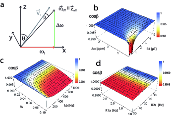
Figure 1: (a) Geometry of the vectors in the rotating frame. (b-d) Cosine of the angle $\beta$ between the eigenvector of the smallest eigenvalue and $\vec{\omega}_{\mathit{eff}}$. (b) In the far off-resonant case both vectors are parallel. Near resonance $\omega_{1}$ has to be strong to keep them parallel. (c) The assumption of collinearity is still valid if pool b with relative concentration $f_{b}<10\%$ is coupled to the water pool. (d) Large differences in $R_{2a}$ and $R_{1a}$ lead to an increasing angle between the vectors, but even for $R_{2a}\approx 50Hz$ and $R_{1a}\approx 1$Hz both vectors are still collinear in good approximation. The eigenvector and the effective field vector are collinear if $\omega_{\mathit{eff}}$ is large compared to $(R_{2a}-R_{1a})$ (A) and $f_{b}<10\%$ – both is fulfilled for CEST experiments since metabolite concentrations are small and frequency offsets of interest are mostly larger than several 100 rad/s.

The collinearity of the corresponding eigenvector and the effective field is the principal reason why off-resonant SL and CEST exhibit the same dynamics. For an appropriate analysis of a saturation experiment it is mandatory to identify the initial projections on the eigenvectors and the measured components. $\vec{B}_{0}$ and $\vec{M}_{0}$ are parallel to the z-axis, the preparation is a projection of the longitudinal magnetization along z onto the effective frame

$$M_{z_{\mathit{eff}}}(t=0) =\cos{\theta}\cdot M_{z}(t=0)=P_{z_{\mathit{eff}}}\cdot M_{0},$$ (5)

$$M_{x_{\mathit{eff}}}(t=0) =\sin{\theta}\cdot M_{0};\quad M_{y_{\mathit{eff}}}(t=0)=0.$$ (6)

The transversal components induce an oscillation decaying with $T_{2\rho}$ [20] which can be neglected in the case of small $\theta$, by averaging over a complete cycle of $\omega_{\mathit{eff}}$, or by measuring after a delay of $~{}5\cdot T_{2\rho}$. This simplification leads to the relation for the back projection, via $P_{z}$, from $z_{\mathit{eff}}$ to z

$$M_{z}(t)=\cos{\theta}\cdot M_{z_{\mathit{eff}}}(t)=P_{z}\cdot M_{z_{\mathit{eff}}}(t).$$ (7)

Since we identified the effective frame as the eigenspace of the magnetization, Eq. (4) can be written as an exponential decay law with the eigenvalue $\lambda_{1}$ associated with the $z_{\mathit{eff}}$ direction. Let the normalized magnetization be $Z=\frac{M_{\mathit{z,a}}}{M_{\mathit{0,a}}}$ and, for the stationary solution, ${Z^{\mathit{ss}}}=\frac{{M}^{\mathit{ss}}_{\mathit{z,a}}}{M_{\mathit{0,a}}}$. Then Eq. (4), taken for the $z_{\mathit{eff}}$ direction, yields the dynamic solution for the z-magnetization

$$Z(\Delta\omega,\omega_{1},t)=(P_{z}P_{z_{\mathit{eff}}}-{Z^{\mathit{ss}}})\cdot e^{\lambda_{1}\cdot t}+{Z^{\mathit{ss}}}$$ (8)

Without preparation pulses $P_{z}=P_{z_{\mathit{eff}}}\approx\cos{\theta}$ (CEST experiment). If a preparation pulse with flip angle $\theta$ is applied before and after cw irradiation the projection factors are $P_{z}=P_{z_{\mathit{eff}}}\approx 1$ (SL experiment), hence oscillations are suppressed (Fig. 2), but still persist since $z_{\mathit{eff}}$ is not perfectly collinear with the eigenvector. Transformation of Eq. (1) into the effective frame and setting $\frac{\text{d}}{\text{d}t}\vec{M}=0$ yields the steady-state solution (A)

$${Z^{\mathit{ss}}}(\Delta\omega,\omega_{1})=-\frac{P_{z}\cdot R_{1a}\cdot\cos{\theta}}{\lambda_{1}}.$$ (9)

It is important to note that in the case where the steady-state is non-zero, it is locked along the corresponding eigenvector. Equations (8) and (9) agree with the full solution previously found for SL by Jin et al. [5] but extend it for CEST.

To obtain a pure dynamic quantity independent of the steady-state we rearrange Eq.(8) and define

$$\tilde{Z}(\Delta\omega,\omega_{1},t)\equiv\frac{Z-{Z^{\mathit{ss}}}}{P_{z}P_{z_{\mathit{eff}}}-{Z^{\mathit{ss}}}}=e^{\lambda_{1}\cdot t}.$$ (10)

Eqs. (9) and (10) are the central formulas in this article.

In fact, the description of SL and CEST experiments differs in the projection factors $P_{z}$ and $P_{z_{\mathit{eff}}}$. The intuitive solution $Z_{CEST}=\cos{\theta}\cdot Z_{SL}$ is valid for the steady-state, but not for the transient-state. If the initial magnetization $M_{i}$ is not fully relaxed and flipped before the saturation pulse by an angle $\beta$, $P_{z_{\mathit{eff}}}$ changes to $\cos(\theta-\beta)\cdot{M_{i}/M_{0}}$.

After understanding of the transition between the two experiments we will now solve the dynamics of CEST and SL experiments by finding the corresponding eigenvalue and verify it numerically.

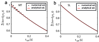
Figure 2: The full numerical Bloch-McConnell solution (dots) with the proposed normalization (Eq. (10)) demonstrates the equivalence of two experiments: chemical exchange saturation transfer (CEST) without preparation pulses (a); spin-lock (SL) with preparation and measurement in the effective frame (b). $\tilde{Z}$ of CEST undergoes oscillations because of residual transversal magnetization in the effective frame. SL shows no oscillations since the transversal magnetization in the effective frame is zero [$\Delta\tilde{Z}$ = 0, see text] (Eq. (24)). Both, SL and CEST, show the same monoexponential decay of the z-magnetization with $\lambda_{1}$ (Eq. (14)) (solid red). For full BM simulations [21] parameters were taken from the amide proton system [3] in brain white matter [22] at $B_{0}$ = 3 T: If not varied, $R_{2a}=14.5$ Hz, $R_{1a}=R_{1b}=0.954$ Hz, $R_{2b}=66.6$ Hz, $f_{b}=1$ %, $k_{b}=25$ Hz, $\delta_{b}=3.5$ ppm, $B_{1}=1~{}\mathrm{\mu T}$, $t_{\mathit{sat}}=1$ s.

As already demonstrated for the SL experiment [14], the eigenvalue, which corresponds to the eigenvector along the $z_{\mathit{eff}}$-axis, is the smallest eigenvalue in modulus of the system. Assuming that all eigenvalues of an arbitrary full-rank matrix $\mathbf{A}$ are much larger in modulus than the smallest eigenvalue, i.e. $|\lambda_{1}|\ll|\lambda_{2...n}|$, we obtain (see B)

$$\lambda_{1}\approx-\frac{c_{0}}{c_{1}},$$ (11)

where $c_{0}$ and $c_{1}$ are the coefficients of the constant and the linear term of the normalized characteristic polynomial, respectively. We derive the full solution for the smallest eigenvalue by employing the solution of the unperturbed system $(f_{b}=0)$. The solution is $\lambda_{\mathit{eff}}=-R_{\mathit{eff}}$ with the decay rate in the effective frame $R_{\mathit{eff}}$ which was shown to be approximately [19]

$$-R_{\mathit{eff}}=R_{1a}\cos^{2}{\theta}+R_{2a}\sin^{2}{\theta}.$$ (12)

With this eigenvalue of the unperturbed system we can rescale the system by

$$\mathbf{A^{\prime}}=\mathbf{A}-\mathbf{I}\cdot\lambda_{\mathit{eff}}$$ (13)

thus shifting the smallest eigenvalue by $R_{\mathit{eff}}$. The smallest eigenvalue of $\mathbf{A^{\prime}}$, still contains terms of $R_{1a}$ and $R_{2a}$, but represents the exchange-induced perturbation of $R_{1\rho}$.

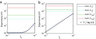
Figure 3: Hierarchy of numerically calculated BM eigenvalues (lines) of the standard system (see caption of Fig. 2). (b) The rescaled matrix $\mathbf{A^{\prime}}$ (eq. (13)) has a much stronger hierarchy in the eigenvalues than matrix $\mathbf{A}$ (a). This improves the approximation of the smallest eigenvalue (x, Eq. (11)).

The result is a strong hierarchy (Fig. 3) in the eigenvalues of $\mathbf{A^{\prime}}$ if the coupling is small ($f_{b}\ll 1$). Now Eq. (11) can be employed to calculate the eigenvalue $\lambda_{1}^{\prime}$ of the matrix $\mathbf{A^{\prime}}$ to obtain the full solution:

$$\lambda_{1}=\lambda_{\mathit{eff}}+\lambda_{1}^{\prime}.$$ (14)

Here $\lambda_{1}^{\prime}=-c_{0}^{\prime}/c_{1}^{\prime}$ is the ratio of the coefficients of the characteristic polynomial of the matrix $\mathbf{A^{\prime}}$. This analytical procedure gives us a very good approximation of the dynamics of the BM system.

For further simplification we assume that relaxation of pool a is well described by $R_{\mathit{eff}}$ and the perturbation is dominated by the exchange and relaxation of pool b. We call the exchange-dependent relaxation rate $R_{\mathit{ex}}=-\lambda_{1}^{\prime}$. The eigenvalue $\lambda_{1}$ is associated with $z_{\mathit{eff}}$ and is therefore an approximation of the relaxation rate in the rotating frame $R_{1\rho}\approx-\lambda_{1}$ given by Eqs. (12) and (14)

$$R_{1\rho}(\Delta\omega)=R_{\mathit{eff}}(\Delta\omega)+R_{\mathit{ex}}(\Delta\omega).$$ (15)

To derive a useful approximation of $R_{\mathit{ex}}$, we neglect all relaxation terms of pool a in matrix $\mathbf{A^{\prime}}$. Furthermore, we assume that $R_{1b}$ is much smaller than $R_{2b}$ and $k_{b}$ and therefore $R_{1b}$ can be neglected in $\mathbf{A^{\prime}}$. In contrast to Trott and Palmer [14], we do not neglect $R_{2b}$, but $k_{a}$. By this means, the obtained eigenvalue approximation by using Eq. (11) is linearized in the small parameter $f_{b}$ giving

$$R_{\mathit{ex}}(\Delta\omega_{b})=\frac{R_{\mathit{ex}}^{\mathit{max}}\frac{\Gamma^{2}}{4}}{\frac{\Gamma^{2}}{4}+\Delta\omega_{b}^{2}}$$ (16)

with maximum value

$$R_{\mathit{ex}}^{\mathit{max}}=f_{b}k_{b}\sin^{2}{\theta}\frac{(\omega_{b}-\omega_{a})^{2}+\frac{R_{2b}}{k_{b}}(\omega_{1}^{2}+\Delta\omega^{2})+R_{2b}(k_{b}+R_{2b})}{\frac{\Gamma^{2}}{4}}$$ (17)

and full width at half maximum (FWHM)

$$\Gamma=2\sqrt{\frac{k_{b}+R_{2b}}{k_{b}}\omega_{1}^{2}+(k_{b}+R_{2b})^{2}}.$$ (18)

For large $|\omega_{b}-\omega_{a}|$

$$R_{\mathit{ex}}^{\mathit{max}}\approx f_{b}k_{b}\cdot\frac{\omega_{1}^{2}}{\omega_{1}^{2}+k_{b}(k_{b}+R_{2b})}.$$ (19)

The $\omega_{1}$-dependent factor yields the amount of labeling of pool b. Hence, we call this factor labeling efficiency, refering to [23]:

$$\alpha=\frac{\omega_{1}^{2}}{\omega_{1}^{2}+k_{b}(k_{b}+R_{2b})}.$$ (20)

For strong $B_{1}$ and small $R_{2b}$ and $k_{b}$, $\alpha$ is approximately one and we obtain the full-saturation limit

$$R_{\mathit{ex}}^{\mathit{max}}\approx f_{b}k_{b}=k_{a}.$$ (21)

3 Results

We obtained numerical values for the eigenvalues computed by means of the full numerical BM matrix solution [21] and compared them to the proposed approximations via

$$R_{\mathit{ex}}=-|\lambda_{1,\text{numerical}}|-R_{\mathit{eff}}.$$ (22)

To verify equations (10,9,14,17) the dynamics of the magnetization vectors of the exchanging spin pools were simulated. The decay rate $R_{\mathit{ex}}$ is obtained from $\tilde{Z}$ (Eq. (10) ) and $R_{\mathit{eff}}$ via

$$R_{\mathit{ex}}=-\frac{\log(\tilde{Z})}{t_{\mathit{sat}}}-R_{\mathit{eff}}.$$ (23)

The simulation parameters for the abundant pool were chosen according to published data for brain white matter [22] including a rare pool attributed to amide protons [2].

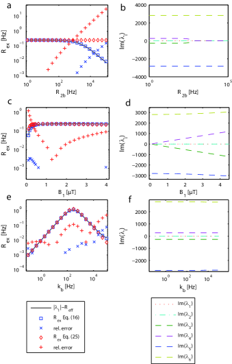
Figure 4: (a,c,e) $R_{\mathit{ex}}$ on-resonant on pool b from smallest eigenvalue in modulus (Eq. (22)) , calculated numerically (line) and analytically by the approximations of Eq. (16) (squares) and the asymmetric population limit of Trott and Palmer [14] (Eq. (25), diamonds). x and + mark the relative error $(1-(R_{\mathit{ex}}^{ana}/R_{\mathit{ex}}^{num}))$ when it is larger than 0.1 %. (a) For small $R_{2b}$, both solutions for $R_{\mathit{ex}}$ agree with the numerical value; if $R_{2b}$ is larger than $k_{b}$ the proposed solution still matches the numerical value. The extension by $R_{2b}$ is important if the CEST pool is not fully saturated, which is the case for small $B_{1}$ (c) or large $k_{b}$ (e). But also for large $B_{1}$ the solution, that includes $R_{2b}$ fits the numerical value with higher accuracy. (b,d,f) Imaginary parts of the numerical eigenvalues. $B_{1}$ and $R_{2b}$ ranges where Eq. (16) (squares) shows deviations from the numerical solution correlate with ranges where the imaginary part becomes small or even zero. In this case, the assumption of a strong hierarchy in the eigenvalues is not valid anymore.

The proposed approximation of $R_{\mathit{ex}}$ by Eq.(16) was compared to the asymmetric population solution of Ref.[14] (Fig. 4). If $R_{2b}$ is non-zero, $R_{\mathit{ex}}$ proposed by Eq.(16) matches the numerical value better than the $R_{\mathit{ex}}$ given in Ref.[14] (see Eq. (25) below). Especially the dependence of $R_{\mathit{ex}}$ on $B_{1}$ (Fig. 4c) changes by taking $R_{2b}$ into account.

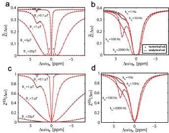
Figure 5: Numerical simulations (dots) of an CEST experiment evaluated for dynamic $\tilde{Z}$-spectra (a, b) and steady-state Z-spectra (c, d) are in agreement with Eqs. (10) and (9) (solid red), respectively. Plots demonstrate high correlation for different $B_{1}(0.1-20~{}\mathrm{\mu T};a,c)$ and $k_{b}(1-2000~{}\mathrm{Hz};b,d)$. Deviations near resonance of pool a for large $B_{1}$ (a) are caused by oscillations of the magnetization in the transverse plane of the effective frame. In the SL experiment these oscillations are suppressed (Fig. 2).

For an CEST experiment, the normalized numerical solution agrees with the theory of dynamic $\tilde{Z}$-spectra (Fig. 5a, b) and steady-state Z-spectra (Fig. 5c, d) for different values of $B_{1}$ and $k_{b}$. The competing direct and exchange-dependent saturation – a central problem in proton CEST [15, 23, 24] – is modeled correctly. Deviations in Fig. 5a for strong $B_{1}$ and $\Delta\omega\rightarrow 0$ result from transversal magnetization in the effective frame which was neglected before. By projection on the transverse plane of the effective frame using Eqs. (6) we obtained the resulting deviation of $\tilde{Z}$

$$\Delta\tilde{Z}(\Delta\omega,\omega_{1},t)=\frac{P_{x}P_{x_{\mathit{eff}}}}{P_{z}P_{z_{\mathit{eff}}}-Z_{ss}}\cdot Re(e^{\lambda_{2}\cdot t}),$$ (24)

with projections $P_{x_{\mathit{eff}}}$ and $P_{x}$ into the transverse plane of the effective frame and back. For MT $P_{x}=P_{x_{\mathit{eff}}}=\sin{\theta}$. Real and imaginary parts of the complex eigenvalue $\lambda_{2}$ are given by $-R_{2\rho}\approx-\frac{1}{2}(R_{2a}+R_{1a}\sin^{2}{\theta}+R_{2a}\cos^{2}{\theta})$ [20] and $\omega_{\mathit{eff}}$, respectively. The implicit neglect of $\Delta\tilde{Z}$ in Eq. (10) is justified if $t_{\mathit{sat}}\gg T_{2\rho}$ or $P_{x}$ and $P_{x_{\mathit{eff}}}$ are small. This can be realized either by SL preparation or by $\omega_{1}\ll\Delta\omega$. The on-resonant case of CEST $(\theta=90^{\circ})$ is not defined, because ${Z^{\mathit{ss}}}$ in Eq. (9) and thus the denominators in Eqs. (10) and (24) vanish. Then the z-axis lies in the transverse plane of the effective frame and Z is described by $M_{\mathit{0,a}}\cdot Re(e^{(-(R_{2\rho}+i\omega_{1})t)})$. Therefore, near resonance SL is preferable to CEST; it also yields in general a higher SNR (given by the projection factors $P_{z}$, $P_{z_{\mathit{eff}}}$). Regarding the experimental realization, CEST is simpler than SL, because $\Delta\omega$ and $\omega_{1}$ and thus $\theta$ can be corrected effectively after the measurement by $B_{0}$ and $B_{1}$ field mapping [23, 25]. In contrast, SL requires knowledge of $B_{1}$ and $B_{0}$ during the scan for proper preparation or techniques that are insensitive to field inhomogeneities such as adiabatic pulses [26, 27].

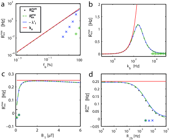
Figure 6: Numerical $R_{\mathit{ex}}^{\mathit{max}}$ (dots), employing Eq. (23), fit to $-\lambda_{1}^{\prime}$ of Eq. (14) (solid blue) and to $R_{\mathit{ex}}^{\mathit{max}}$ of Eq. (17) (dashed green) as a function of $f_{b}$, $k_{b}$, $B_{1}$, and $R_{2b}$. x and + mark the relative error $(1-(R_{\mathit{ex}}^{ana}/R_{\mathit{ex}}^{num}))$ when it is larger than 1 %. (a) As expected, the eigenvalue approximation is insufficient for $f_{b}>5\%$. (b) Contrary to the approximation of Eq.(21) (solid red) the full solution follows the decrease of $R_{\mathit{ex}}^{\mathit{max}}$ with large $k_{b}$. The decrease of deviations for small $B_{1}$ (c) and high $R_{2b}$ (d) may be caused by overdamping in pool b, i.e., eigenvalues become real which reduces the required hierarchy in the set of the eigenvalues. However, the deviation in $R_{\mathit{ex}}$ is too small (Fig. 4) to explain this deviation leading to the conclusion that other eigenvectors are contributing to the relaxation. (d) Inclusion of $R_{2b}$ is relevant for $R_{2b}>100$ Hz.

The values of the rate $R_{\mathit{ex}}^{\mathit{max}}$ obtained by simulations fit well to the full (Eq. (14)) and approximate (Eq. (17)) solution for the observed parameters (Fig. 6). Deviations of simulation and analytical solution were smaller than 1% for rates varied in the ranges: $R_{1b}=0.1-10$ Hz, $R_{1a}=0.1-10$ Hz and $R_{2a}=2-100$ Hz (data not shown).

4 Discussion

4.1 General solution

We showed that our formalism, established by Eqs. (10),(9) and (8) together with the eigenvalue approximation of Eq. (14), is a general solution for CEST experiments. This now allows us to discuss from a general point of view the techniques and theories proposed in the field of chemical exchange saturation transfer. For the SL solution this was already accomplished by Jin et al. [12, 5].

The proposed eigenvalue approximation assumes the case of asymmetric populations. This restricts its application to systems where the water proton pool is much larger than the exchanging pools – which is the case for CEST experiments. There are many analytical approaches for the smallest eigenvalue ($R_{1\rho}$) of the BM matrix besides our approach. They use pertubation theory [19], the stochastic Liouville equation [28], an average magnetization approach [29], and the polynomial root finding algorithm of Laguerre [18]. The latter is even valid in the case of symmetric populations. However, all these treatments neglect the transverse relaxation of the exchanging pool. Since in CEST experiments the exchange rates are often quite small (e.g., $k_{b}\approx 28Hz$ for APT), $R_{2b}$ cannot be neglected against $k_{b}$. We chose therefore a simple approach which is suitable for the condition of asymmetric populations and took $R_{2b}$ into account. Our approach to find the eigenvalue including $R_{2b}$ is similar to that of Trott and Palmer [14]. However, different $R_{1}$ and $R_{2}$ were allowed for the involved pools. In addition, an alternative justification of the relation $\lambda_{1}=-\frac{c_{0}}{c_{1}}$ was obtained, which uses the intrinsic hierarchy of the eigenvalues (B) instead of linearization of the characteristic polynomial. By this means, it turned out that a strong hierarchy of the eigenvalues is necessary for the approximation. The hierarchy was increased by rescaling the system by the unperturbed eigenvalue $R_{\mathit{eff}}$ (Fig.3). Thus the accuracy of the approximation was improved. As the parameter $R_{2b}$ was included and equations were linearized directly in the small parameter $k_{a}$, a formula was obtained (Eq. (15)) that differs from the asymmetric population limit of Ref. [14] reading

$$R_{1\rho}=R_{\mathit{eff}}+\underbrace{\sin^{2}{\theta}\frac{(\omega_{b}-\omega_{a})^{2}\frac{k_{a}k_{b}}{k_{a}+k_{b}}}{\Delta\omega_{b}^{2}+\omega_{1}^{2}+(k_{a}+k_{b})^{2}}}_{R_{\mathit{ex}}}.$$ (25)

Equality is reached if $R_{2b}$ is neglected in our approximation and if Eq. (25) is linearized in $k_{a}$. With our extension simulated CEST Z-spectra could be predicted well in a broad range of parameters. Moreover, it turned out that $R_{2b}$ is important if it is in the range of $k_{b}$ (Fig. 6d). Inclusion of $R_{2b}$ also allows to model macromolecular magnetization transfer effects with large $R_{2b}$ values (Fig. 8c).

Our solution agrees for SL with the existing treatment [12], but only with the correct projection factors SL and CEST can be described by the same theory. This is contrary to the conclusion of Jin et al. [12] that SL theory can be used directly to describe CEST experiments. The deviation is not large for small $\theta$, but for $\omega_{1}\approx\Delta\omega$ the projection factors are crucial as shown in Fig. 7.

With the correct projections the transition to CEST is straightforward and provides a much broader range of validity than previous models developed for CEST which are either appropriate only for small $B_{1}$ [24] or large $B_{1}$ [30] or only for the case of on-resonant irradiation of pool b [23, 15]. The proposed theory (Eq. (8)) gives a model for full Z-spectra for transient and steady-state CEST experiments which enables analytical rather than numerical fitting of experimental data.

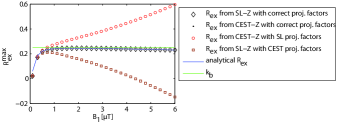
Figure 7: The same plot of $R_{\mathit{ex}}^{\mathit{max}}$ (Eq. (23)) as in Fig. 6c, but now for CEST (dots) and SL (diamonds) employing the corresponding projection factors in Eq. (10) ($P_{z}=P_{z_{\mathit{eff}}}=1$ for SL and $P_{z}=P_{z_{\mathit{eff}}}=\cos\theta$ for CEST). Additionally, the result of an evaluation is shown employing the projection factors of SL for a CEST experiment (circles) and employing the projection factors of CEST for a SL experiment (squares). Only with the correct projection factors both experiments are described by the same theory and yield $R_{\mathit{ex}}$ (solid blue).

4.2 Extension to other systems

As verified for SL [19], the theory can be extended to $n$-site exchanging systems. By simply superimposing the exchange-dependent relaxation rates of several pools one obtains the Z-spectra for a multi-pool system. We applied this to the contrast agent iopamidol in water, which has two exchanging amide proton groups [31], considering a three pool system: water, amide proton B at 4.2 ppm and amide proton C at 5.5 ppm. Assuming for the exchange rates $k_{c}=6\cdot k_{b}$, the superposition of $R_{\mathit{eff}}$ and the two corresponding $R_{\mathit{ex}}$ yields the Z-spectrum of the iopamidol system (Fig. 8a). A three-pool system relevant for in vivo CEST studies includes water protons, amide protons and a macromolecular proton pool. Modeling the macromolecular pool by $R_{\mathit{ex}}^{m}$($R_{2m}$ = 5000 Hz, $k_{m}$ = 40 Hz) with an offset of -2.6 ppm and again superimposing it with $R_{\mathit{ex}}^{amide}$ we are able to model analytically Z-spectra of APT with an underlying symmetric and asymmetric MT effect up to 5% relative concentration $f_{m}$ (Fig. 8b). Hence, the model is able to describe the in vivo situation of several CEST pools and underlying MT competing with direct water saturation. Using the superimposed $R_{\mathit{ex}}$ including $R_{\mathit{ex}}^{m}$ and $R_{\mathit{ex}}^{amide}$ and fitting the obtained Z-spectra $R_{\mathit{ex}}^{amide}$ can be isolated. For macromolecular MT the extension of $R_{\mathit{ex}}$ by $R_{2b}$ is crucial, since $R_{2b}$ can be as large as $\approx 10^{5}$ Hz. The implicitly assumed Lorentzian lineshape of the macromolecular pool is only valid around the water proton resonance, for large offsets a super-Lorentzian lineshape must be included in $R_{\mathit{ex}}^{m}$ [22].

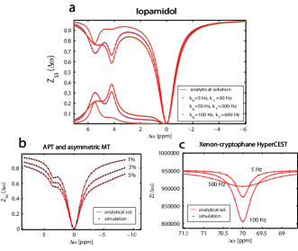
Figure 8: Three applications of the proposed theory:(a) The system of iopamidol with corresponding $\mathrm{MTR}_{\mathrm{asym}}$ evaluation. (b) The system of APT with an asymmetric macromolecular MT pool (for concentration fractions $f_{m}$ =1%, 3%, 5%). (c) The system of exchanging hyperpolarized xenon soluted or encapsulated in cryptophane cages, a biosensor method called HyperCEST.

Hyperpolarized xenon spin ensembles exchanging between the dissolved phase and cryptophane cages (HyperCEST experiment, [32]) can also be described by Eq. (10). Since the initial hyperpolarized magnetization $M_{i}$ is in the order up to $10^{5}...10^{6}M_{0}$, the steady-state can be neglected for depolarization. This yields $Z\approx\tilde{Z}=M_{i}\cdot e^{-R_{1\rho}t_{\mathit{sat}}}$ in agreement with the result in Ref. [33]. Figure  8c shows the simulated Z-spectrum around the cage peak in the HyperCEST experiment of a Xe-cryptophane system for different $k_{b}$.

Pulsed irradiation, employed for saturation in SAR limited clinical scanners [34], was shown to have similar effects on $\mathrm{MTR}_{\mathrm{asym}}$ as cw irradiation with effective $B_{1}$ [35, 36]. The presented solution for CEST Z-spectra can therefore be used for optimization of pulsed saturation transfer experiments.

4.3 Proton transfer ratio

For a CEST experiment the parameters of particular interest are the exchange rate $k_{b}$ of the metabolite proton pool and the relative concentration $f_{b}$. The former is often pH catalyzed and permits pH-weighted imaging; the latter allows molecular imaging with enhanced sensitivity. The ultimate method must allow – with high spectral selectivity – the generation of $k_{b}$ and $f_{b}$ maps separately and for different exchanging groups. Unfortunately, both parameters occur in the water pool BM equations as product, i.e. the back-exchange rate $k_{a}=k_{b}\cdot f_{b}$. There are some approaches which are able to separate $k_{b}$ and $f_{b}$ for specific cases like rotation transfer of amid protons [37] or the method of Dixon et al. [38] applicable to PARACEST agents. CEST experiments are commonly evaluated to yield the proton transfer ratio PTR. PTR is an ideal parameter in the sense that it reflects the decrease of the water pool signal owing to exchange from a labeled exchanging pool only, thus neglecting any direct saturation.

In the following, we assume one CEST pool resonance on the positive $\Delta\omega$ axis.

Employing Eq. (9) with the limit $\theta\rightarrow 0$ we obtain for PTR in steady-state:

$$\text{PTR}=1-{Z^{\mathit{ss}}}(\Delta\omega)\approx\frac{R_{\mathit{ex}}(+\Delta\omega)}{R_{1a}+R_{\mathit{ex}}(+\Delta\omega)}$$ (26)

which yields the maximal value $\frac{k_{a}}{R_{1a}+k_{a}}$ [2] in the full-saturation limit ($R_{\mathit{ex}}\approx k_{a}$ ). Eq. (26) is consistent with PTR including the labeling efficiency $\alpha$ introduced in Ref. [23].

4.4 Z-spectra evaluation - $\mathrm{MTR}$ and $\mathrm{MTR}_{\mathrm{asym}}$

Methods using asymmetry implicitly assume that the full width at half maximum of $R_{\mathit{ex}}$ ($\Delta\omega_{b}$) is narrow compared to the chemical shift of the corresponding pool. This means that $R_{\mathit{ex}}$ ($\Delta\omega_{b}$) can be neglected for the reference scan $Z(-\Delta\omega)$ what is only true in the slow-exchange limit [2]. This limit can be defined more generally by the width of $R_{\mathit{ex}}$ ($\Delta\omega_{b}$) (Eq. (18)):

$$\Gamma=2\sqrt{\frac{k_{b}+R_{2b}}{k_{b}}\cdot\omega_{1}^{2}+(k_{b}+R_{2b})^{2}}\ll|\Delta\omega_{b}-\Delta\omega_{a}|$$ (27)

This new limit depends on $B_{1}$ which affects the ability to distinguish different peaks in the Z-spectrum (Fig. 5c). The limit is therefore a useful parameter for exchange-regime characterization in saturation spectroscopy.

For CEST the common evaluation parameters are the magnetization transfer rate $\mathrm{MTR}(\Delta\omega)=1-Z(\Delta\omega)$ and the asymmetry of the Z-spectrum $\mathrm{MTR}_{\mathrm{asym}}(\Delta\omega)=Z(-\Delta\omega)-Z(+\Delta\omega)$. $\mathrm{MTR}_{\mathrm{asym}}$ is generally employed to estimate PTR. Using Eq. (9) together with Eq. (15) we obtain for steady-state Z-spectrum asymmetry

$$\begin{split}\mathrm{MTR}_{\mathrm{asym}}^{\mathit{ss}}(\Delta\omega)&={Z^{\mathit{ss}}}(-\Delta\omega)-{Z^{\mathit{ss}}}(+\Delta\omega)\\ &=\frac{(R_{\mathit{ex}}(+\Delta\omega)-R_{\mathit{ex}}(-\Delta\omega))\cdot R_{1a}P_{z}\cos{\theta}}{(R_{\mathit{eff}}+R_{\mathit{ex}}(-\Delta\omega))(R_{\mathit{eff}}+R_{\mathit{ex}}(+\Delta\omega))}.\end{split}$$ (28)

The comparison shows that $\mathrm{MTR}_{\mathrm{asym}}^{\mathit{ss}}$ yields PTR of Eq. (26) only if $\theta=0$.

Sun et al. [15] found $\mathrm{MTR}_{\mathrm{asym}}^{\mathit{ss}}=PTR\cdot\alpha\cdot(1-\sigma)$ which combines the labeling efficiency $\alpha$ found by the weak-saturation-pulse approximation and a spillover coefficient $\sigma$ from the strong-saturation-pulse approximation. This formula is only valid on resonance of pool b in contrast to Eq. (28).

Another approach, applicable for small $B_{1}$, eliminates the spillover effect by a probabilistic approach [24]. This Z-spectrum model taken from [24] yields

$$\begin{split}\text{PTR}(\Delta\omega)&\approx\frac{{Z^{\mathit{ss}}(-\Delta\omega)}-{Z^{\mathit{ss}}(+\Delta\omega)}}{{Z^{\mathit{ss}}(-\Delta\omega)}-{Z^{\mathit{ss}}(+\Delta\omega)}+{Z^{\mathit{ss}}(-\Delta\omega)}\cdot{Z^{\mathit{ss}}(+\Delta\omega)}}\\ &=\frac{R_{\mathit{ex}}(+\Delta\omega)}{\cos^{2}\theta\cdot R_{1a}+R_{\mathit{ex}}(+\Delta\omega)}\end{split}$$ (29)

which turns out, after substitution of ${Z^{\mathit{ss}}}$ by Eq.(9), to be an approximation of PTR if $\theta$ is small. The asymmetry normalized by the reference scan was proposed for spillover correction [39]. Applying eq. (9) yields

$$\frac{{Z^{\mathit{ss}}}(-\Delta\omega)-{Z^{\mathit{ss}}(+\Delta\omega)}}{{Z^{\mathit{ss}}(-\Delta\omega)}}=\frac{R_{\mathit{ex}}(+\Delta\omega)}{R_{\mathit{eff}}(+\Delta\omega)+R_{\mathit{ex}}(+\Delta\omega)}$$ (30)

which again approximates PTR if $\theta$ is small.

By use of Eqs. (9) and (8) we obtain for the asymmetry in transient-state a bi-exponential function

$$\begin{split}\mathrm{MTR}_{\mathrm{asym}}(\Delta\omega,t)=&\mathrm{MTR}_{\mathrm{asym}}^{\mathit{ss}}(\Delta\omega)\\ +e^{-R_{1\rho}(-\Delta\omega)t}\cdot&(P_{z}P_{z_{\mathit{eff}}}-Z^{ss}(-\Delta\omega))\\ -e^{-R_{1\rho}(+\Delta\omega)t}\cdot&(P_{z}P_{z_{\mathit{eff}}}-Z^{ss}(+\Delta\omega)).\end{split}$$ (31)

Neglecting direct saturation of pool a and assuming $P_{z}$ = $P_{z_{\mathit{eff}}}$ = 1 yields the mono-exponential approximation at the CEST resonance [2, 40]

$$\mathrm{MTR}_{\mathrm{asym}}(\Delta\omega_{b}=0,t)=\mathrm{MTR}_{\mathrm{asym}}^{\mathit{ss}}(\Delta\omega_{b}=0)\cdot(1-e^{-(R_{1a}+k_{a})t}),$$ (32)

with the rate constant $R_{1\rho}=R_{1a}+k_{a}$. This is valid if $\theta$ is small, leading to $R_{\mathit{eff}}\approx R_{1a}$ and, with the limit of Eq. (21), $R_{\mathit{ex}}\approx k_{a}$ (solid red, Fig. 6b).

The ratiometric analysis approach QUESTRA [41] includes direct saturation and is independent of steady-state. It can be expressed by means of Eq. (10) under the same assumptions $P_{z}$ =$P_{z_{\mathit{eff}}}$ =1 and $R_{\mathit{eff}}\approx R_{1a}$ and $R_{\mathit{ex}}\approx k_{a}$

$$\text{QUESTRA}(t)=\frac{\tilde{Z}(+\Delta\omega,t)}{\tilde{Z}(-\Delta\omega,t)}\approx e^{-k_{a}t}.$$ (33)

Another method, pCEST [13], employs $R_{1\rho}$ in an inversion recovery experiment. The pCEST signal obeys the negative of Eq. (31) if the initial inversion is introduced by $P_{z_{\mathit{eff}}}=-\cos\theta$. Hence, the full dynamics of the $R_{1\rho}$ inversion recovery signal is

$${\color[rgb]{0,0,0}\text{pCEST}(\Delta\omega,t)=-\mathrm{MTR}_{\mathrm{asym}}(\Delta\omega,t,P_{z_{\mathit{eff}}}=-\cos\theta)}$$ (34)

The pCEST signal can be positive in transient-state, but is negative in steady-state. This inversion recovery approach was suggested first to increase SNR for MT effect by Mangia et al. [42] and for SL already by Santyr et al. [43] and again by Jin and Kim [44]. Their iSL signal is in our notation equal to $Z$ ($\Delta\omega$,$\omega_{1}$,t) (Eq.(8)) with $P_{z_{\mathit{eff}}}$ =-1 and their projection factors for CEST and SL are identical with $P_{z}$ and $P_{z_{\mathit{eff}}}$. For $R_{\mathit{ex}}$ the approximation of Ref. [14] is used, assuming $R_{2b}=R_{2a}$. Especially for the quantification employing different $B_{1}$ their approach will benefit from our approximation of $R_{\mathit{ex}}$. By irradiation with Toggling Inversion Preparation (iTIP) Jin and Kim were able to remove ${Z^{\mathit{ss}}}$ which allows for direct exponential fit of the difference signal of SL and iSL and thus promises reduced scanning time [44].

4.5 Separation for $R_{\mathit{ex}}$

The dependence of CEST and SL on exchange is mediated by $R_{\mathit{ex}}$, the exchange-dependent relaxation rate in the rotating frame. Since the discussed evaluation algorithms for PTR depend on direct water saturation, we propose methods which use the underlying structure of the Z-spectrum and solve the solutions for $R_{\mathit{ex}}$. For the transient state QUESTRA can be extended by inclusion of $R_{\mathit{ex}}$ and the projection factors (in $\tilde{Z}$, Eq. (10)) :

$$\text{QUESTRA}_{R_{ex}}(t)=\frac{\tilde{Z}(+\Delta\omega,t)}{\tilde{Z}(-\Delta\omega,t)}=e^{-R_{\mathit{ex}}(\Delta\omega)t}.$$ (35)

which provides direct access to $R_{\mathit{ex}}$. Even without creating $\tilde{Z}$ one can measure the experimental $R_{1\rho}$ ($\Delta\omega$) decay rate and obtains $R_{\mathit{ex}}(\Delta\omega)\approx R_{1\rho}(+\Delta\omega)-R_{1\rho}(-\Delta\omega)$ by asymmetry analysis of the rate $R_{1\rho}$ ($\Delta\omega$). For the evaluation of steady-state measurements we suggest an extension of Eq. (30)

$$\text{MTR}_{R_{ex}}(+\Delta\omega)=\frac{{Z^{\mathit{ss}}(-\Delta\omega)}-{Z^{\mathit{ss}}(+\Delta\omega)}}{{Z^{\mathit{ss}}(-\Delta\omega)}\cdot{Z^{\mathit{ss}}(+\Delta\omega)}}=\\ =\frac{1}{{Z^{\mathit{ss}}(+\Delta\omega)}}-\frac{1}{{Z^{\mathit{ss}}(-\Delta\omega)}}=\frac{R_{\mathit{ex}}(+\Delta\omega)}{\cos\theta\cdot P_{z}\cdot R_{1a}}$$ (36)

which yields $R_{\mathit{ex}}$ in units of $R_{1a}$ and is independent of spillover. $R_{\mathit{ex}}$ can be calculated by determination of $R_{1a}$ and the projection factors . $\theta$ can be determined by $B_{1}$ mapping and $R_{1a}$ can be measured, however $R_{1a}$ is not the same as the observed relaxation rate $R_{\mathit{obs}}$ in a inversion or saturation recovery experiment, especially if a macromolecular pool is present [16]. Since MTR${}_{R_{ex}}$ and QUESTRA${}_{R_{ex}}$ evaluations employ directly Z-spectra data, they are useful saturation transfer evaluation methods for determination of $R_{\mathit{ex}}$ with correction of direct saturation. However, they are still asymmetry-based and are not applicable to systems with pools with opposed resonance frequencies. In this case, the most reliable evaluation is fitting whole Z-spectra by using Eq.(8) including a superimposed $R_{\mathit{ex}}$ of the contributing pools.

4.6 Determination of $R_{2b}$, $k_{b}$ and $f_{b}$

As proposed by Jin et al. [12] the width $\Gamma$ (Eq. (18)) of $R_{\mathit{ex}}$ ($\Delta\omega_{b}$) can be used to obtain $k_{b}$ directly. But especially for small $k_{b}$ the extension by $R_{2b}$ is necessary. Fitting $R_{\mathit{ex}}^{\mathit{max}}$ for different $B_{1}$ yields $f_{b}$ and $k_{b}$ separately similar to the QUESP method [40] and Dixons Omega Plots [38] , but again the neglect of $R_{2b}$ in Eq. (19) will distort the values for $k_{b}$ and $f_{b}$. The width of $R_{\mathit{ex}}$ is a linear function of $\omega_{1}^{2}$:

$$\frac{\Gamma^{2}}{4}(\omega_{1}^{2})=\frac{k_{b}+R_{2b}}{k_{b}}\cdot(\omega_{1}^{2})+(k_{b}+R_{2b})^{2}$$ (37)

and 1/$R_{\mathit{ex}}^{\mathit{max}}$ is a linear function of $\omega_{1}^{-2}$

$$\frac{1}{R_{\mathit{ex}}^{\mathit{max}}(\omega_{1}^{-2})}=\frac{k_{b}+R_{2b}}{f_{b}}\cdot(\omega_{1}^{-2})+\frac{1}{f_{b}k_{b}}.$$ (38)

Hence, also the fit of Z-spectra for different $B_{1}$ yields $f_{b}$, $k_{b}$ and $R_{2b}$, separately.

5 Conclusion

We extended the analytical solution of the BM equations for SL by the relaxation rate $R_{2b}$ and identified the projection factors necessary for application of the theory to CEST experiments. Temporal evolution as well as steady-state magnetization of CEST and SL experiments can be described by one single model governed by the smallest eigenvalue in modulus of the BM equation system which is $-R_{1\rho}$. $R_{1\rho}$ contains the exchange-dependent relaxation rate $R_{\mathit{ex}}$. We extended $R_{\mathit{ex}}$ by the transversal relaxation $R_{2b}$ which allows application of the theory to slow exchange, where $R_{2b}$ is in the order of $k_{b}$ and not negligible. $R_{\mathit{ex}}$ of different pools can be superimposed to a multi-pool model even for a macromolecular MT pool. Compared to methods designed to estimate PTR, estimators of $R_{\mathit{ex}}$ are less dependent on water proton relaxation. Finally, we showed that determination of $R_{\mathit{ex}}$ as a function of $\omega_{1}$ and $\Delta\omega$ allows to determine concentration, exchange rate, and transverse relaxation of the exchanging pool.

Appendix A Eigenvector approximation

We consider the Taylor expansion in $f_{b}$ of the eigenvector $\lambda_{1}$ of the smallest eigenvalue in modulus $\lambda_{1}$. The constant term of this expansion evaluated on the resonance of pool b yields for the components of this eigenvector in pool a

$$\begin{pmatrix}\omega_{1}\\ 0\\ \Delta\omega\end{pmatrix}+\underbrace{\begin{pmatrix}\frac{(R_{1a}+\lambda_{1})(R_{2a}+\lambda_{1})}{\omega_{1}}\\ \frac{\Delta\omega}{\omega_{1}}(R_{1a}+\lambda_{1})\\ 0\end{pmatrix}}_{*}$$ (39)

With the approximation of Eq. (12) $\lambda_{1}=-R_{\mathit{eff}}=R_{1a}+(R_{2a}-R_{1a})\sin^{2}\theta=R_{2a}-(R_{2a}-R_{1a})\cos^{2}\theta$. The first component of (*) can be neglected if

$$|\frac{(R_{1a}-R_{\mathit{eff}})(R_{2a}-R_{\mathit{eff}})}{\omega_{1}}|\ll\omega_{1}.$$ (40)

This yields

$$(R_{2a}-R_{1a})^{2}\ll\frac{\omega_{1}^{2}}{\sin^{2}\theta\cos^{2}\theta}=\frac{\omega_{1}^{2}}{\frac{\omega_{1}^{2}\Delta\omega^{2}}{\omega_{\mathit{eff}}^{4}}}=\frac{\omega_{\mathit{eff}}^{4}}{\Delta\omega^{2}}.$$ (41)

Since $\frac{\omega_{\mathit{eff}}^{4}}{\Delta\omega^{2}}>\omega_{\mathit{eff}}^{2}$ this can be reduced to the condition

$$|R_{2a}-R_{1a}|\ll\omega_{\mathit{eff}}.$$ (42)

The second component of (*) vanishes under the same condition (42). After neglect of (*) and normalization the eigenvector of the smallest eigenvalue (Eq. (39)) simplifies to (Fig. 1a)

$$\vec{v}_{1}=\begin{pmatrix}\sin\theta\\ 0\\ \cos\theta\end{pmatrix}.$$ (43)

Along this eigenvector the Bloch-McConnell equations are one-dimensional

$$\dot{M}_{z_{eff}}=\lambda_{1}\cdot M_{z_{eff}}+C_{z_{eff}}$$ (44)

where the constant part $C_{z_{eff}}$ is the projection of $\vec{C}$ (Eq. (3)) on the eigenvector $\vec{v}_{1}$ (43) giving

$$C_{z_{eff}}=\cos\theta\cdot R_{1a}.$$ (45)

The solution of Eq. (44) is the combination of the general solution of the homogeneous equation (which is an exponential function with rate $\lambda_{1}$) superimposed with a special solution of the inhomogeneous equation. The steady-state is a special solution and is obtained by setting $\dot{M}_{z_{eff}}=0$ which gives

$$-\lambda_{1}\cdot M_{z_{eff}}=\cos\theta\cdot R_{1a}.$$ (46)

By backprojection on the z-axis and normalization by $M_{0}$ one obtains the steady-state solution Eq. (9):

$${Z^{\mathit{ss}}}=\frac{P_{z}R_{1a}\cos\theta}{-\lambda_{1}}$$ (47)

Appendix B Eigenvalue approximation

The eigenvalues $\lambda_{i}$ of a $n\times n$-matrix are the roots of the normalized characteristic polynomial and are defined by

$$\det(\mathbf{A}-\lambda\cdot\mathbf{I})=0\Leftrightarrow\lambda^{n}+c_{n-1}\lambda^{n-1}+...+c_{1}\lambda+c_{0}=0$$ (48)

where

$$c_{0}=(-1)^{n}\det(\mathbf{A})=(-1)^{n}\lambda_{1}\cdot...\cdot\lambda_{n}$$ (49)

and

$$c_{1}=(-1)^{n-1}\sum_{i=1}^{n}\frac{\lambda_{1}\cdot...\cdot\lambda_{n}}{\lambda_{i}}=-c_{0}\cdot\sum_{i=1}^{n}\frac{1}{\lambda_{i}}$$ (50)

The assumption that all eigenvalues are much larger than $|\lambda_{1}|\ll|\lambda_{2}|\leq...\leq|\lambda_{n}|$ leads to

$$c_{1}=-c_{0}\cdot(\frac{1}{\lambda_{1}}+\frac{1}{\lambda_{2}}+...+\frac{1}{\lambda_{n}})\approx-\frac{c_{0}}{\lambda_{1}}$$ (51)

This approximation is also valid for complex eigenvalues, because the conjugate complex is also an eigenvalue and therefore $\frac{1}{\lambda_{j}}+\frac{1}{\lambda_{j}^{*}}=\frac{2Re(\lambda_{j})}{|\lambda_{j}|^{2}}<\frac{2}{|\lambda_{j}|}$. Equations (A.2) and (A.4) allow general approximation of the smallest eigenvalue in modulus by

$$\lambda_{1}=-\frac{c_{0}}{c_{1}}$$ (52)

The error is smaller than $|\frac{\lambda_{1}^{\prime\prime}}{\lambda_{2}^{\prime\prime}\cdot(n-1)}|$. Justified by linearization of the characteristic polynomial, expression (52) was also suggested in Ref. [14].

References

- Wolff and Balaban [1990] S. D. Wolff, R. S. Balaban, NMR imaging of labile proton exchange, J. Magn. Reson. (1969) 86 (1990) 164–169.
- Zhou and Zijl [2006] J. Zhou, P. C. v. Zijl, Chemical exchange saturation transfer imaging and spectroscopy, Progr. Nucl. Magn. Reson. Spect. 48 (2006) 109–136.
- Zhou et al. [2003] J. Zhou, J. Payen, D. A. Wilson, R. J. Traystman, P. C. M. v. Zijl, Using the amide proton signals of intracellular proteins and peptides to detect pH effects in MRI, Nat. Med. 9 (2003) 1085–1090.
- Cai et al. [2012] K. Cai, M. Haris, A. Singh, F. Kogan, J. H. Greenberg, H. Hariharan, J. A. Detre, R. Reddy, Magnetic resonance imaging of glutamate, Nat. Med. 18 (2012) 302–306.
- Jin et al. [2012] T. Jin, P. Wang, X. Zong, S. Kim, Magnetic resonance imaging of the Amine-Proton EXchange (APEX) dependent contrast, NeuroImage 59 (2012) 1218–1227. PMID: 21871570.
- Ling et al. [2008] W. Ling, R. R. Regatte, G. Navon, A. Jerschow, Assessment of glycosaminoglycan concentration in vivo by chemical exchange-dependent saturation transfer (gagCEST), Proceedings of the National Academy of Sciences of the United States of America 105 (2008) 2266–2270. PMID: 18268341.
- Jia et al. [2011] G. Jia, R. Abaza, J. D. Williams, D. L. Zynger, J. Zhou, Z. K. Shah, M. Patel, S. Sammet, L. Wei, R. R. Bahnson, M. V. Knopp, Amide proton transfer MR imaging of prostate cancer: a preliminary study, Journal of Magnetic Resonance Imaging: JMRI 33 (2011) 647–654. PMID: 21563248.
- Schmitt et al. [2011] B. Schmitt, P. Zamecnik, M. Zaiss, E. Rerich, L. Schuster, P. Bachert, H. P. Schlemmer, A new contrast in MR mammography by means of chemical exchange saturation transfer (CEST) imaging at 3 tesla: preliminary results, RoFo 183 (2011) 1030–1036. PMID: 22034086.
- Zhou [2011] J. Zhou, Amide proton transfer imaging of the human brain, Meth. Mol. Bio. 711 (2011) 227–237. PMID: 21279604.
- Gerigk et al. [2012] L. Gerigk, B. Schmitt, B. Stieltjes, F. Roeder, M. Essig, M. Bock, H.-P. Schlemmer, M. Roethke, 7 tesla imaging of cerebral radiation necrosis after arteriovenous malformations treatment using amide proton transfer (APT) imaging, Journal of magnetic resonance imaging: JMRI 35 (2012) 1207–1209. PMID: 22246564.
- Schmitt et al. [2011] B. Schmitt, S. Zbyn, D. Stelzeneder, V. Jellus, D. Paul, L. Lauer, P. Bachert, S. Trattnig, Cartilage quality assessment by using glycosaminoglycan chemical exchange saturation transfer and (23)Na MR imaging at 7 t, Radiology 260 (2011) 257–264. PMID: 21460030.
- Jin et al. [2011] T. Jin, J. Autio, T. Obata, S. Kim, Spin-locking versus chemical exchange saturation transfer MRI for investigating chemical exchange process between water and labile metabolite protons, Magn. Reson. Med. 65 (2011) 1448–1460.
- Vinogradov et al. [2012] E. Vinogradov, T. C. Soesbe, J. A. Balschi, A. D. Sherry, R. E. Lenkinski, pCEST: positive contrast using chemical exchange saturation transfer, Journal of magnetic resonance (San Diego, Calif.: 1997) 215 (2012) 64–73. PMID: 22237630.
- Trott and Palmer [2002] O. Trott, A. G. Palmer, R1rho relaxation outside of the fast-exchange limit, J. Magn. Reson. 154 (2002) 157–160.
- Sun and Sorensen [2008] P. Z. Sun, A. G. Sorensen, Imaging pH using the chemical exchange saturation transfer (CEST) MRI: correction of concomitant RF irradiation effects to quantify CEST MRI for chemical exchange rate and pH, Magn. Reson. Med. 60 (2008) 390–397.
- Desmond and Stanisz [2012] K. L. Desmond, G. J. Stanisz, Understanding quantitative pulsed CEST in the presence of MT, Magnetic Resonance in Medicine: Official Journal of the Society of Magnetic Resonance in Medicine / Society of Magnetic Resonance in Medicine 67 (2012) 979–990. PMID: 21858864.
- McConnell [1958] H. M. McConnell, Reaction rates by nuclear magnetic resonance, J. Chem. Phys. 28 (1958) 430.
- Miloushev and Palmer III [2005] V. Z. Miloushev, A. G. Palmer III, R1rho relaxation for two-site chemical exchange: General approximations and some exact solutions, Journal of Magnetic Resonance 177 (2005) 221–227.
- Trott and Palmer [2004] O. Trott, A. G. Palmer, Theoretical study of r(1rho) rotating-frame and r2 free-precession relaxation in the presence of n-site chemical exchange, J. Magn. Reson. 170 (2004) 104–112.
- Moran and Hamilton [1995] P. R. Moran, C. A. Hamilton, Near-resonance spin-lock contrast, Magn. Reson. Imaging 13 (1995) 837–846.
- Woessner et al. [2005] D. E. Woessner, S. Zhang, M. E. Merritt, A. D. Sherry, Numerical solution of the bloch equations provides insights into the optimum design of PARACEST agents for MRI, Magn. Reson. Med. 53 (2005) 790–799.
- Stanisz et al. [2005] G. J. Stanisz, E. E. Odrobina, J. Pun, M. Escaravage, S. J. Graham, M. J. Bronskill, R. M. Henkelman, T1, t2 relaxation and magnetization transfer in tissue at 3T, Magn. Reson. Med. 54 (2005) 507–512.
- Sun et al. [2007] P. Z. Sun, C. T. Farrar, A. G. Sorensen, Correction for artifacts induced by b(0) and b(1) field inhomogeneities in pH-sensitive chemical exchange saturation transfer (CEST) imaging, Magn. Reson. Med. 58 (2007) 1207–1215.
- Zaiss et al. [2011] M. Zaiss, B. Schmitt, P. Bachert, Quantitative separation of CEST effect from magnetization transfer and spillover effects by lorentzian-line-fit analysis of z-spectra, J. Magn. Reson. 211 (2011) 149–155.
- Kim et al. [2009] M. Kim, J. Gillen, B. A. Landman, J. Zhou, P. C. M. v. Zijl, Water saturation shift referencing (WASSR) for chemical exchange saturation transfer (CEST) experiments, Magn. Reson. Med. 61 (2009) 1441–1450.
- Mangia et al. [2009] S. Mangia, T. Liimatainen, M. Garwood, S. Michaeli, Rotating frame relaxation during adiabatic pulses vs. conventional spin lock: simulations and experimental results at 4 t, Magn. Reson. Imaging 27 (2009) 1074–1087.
- Michaeli et al. [2004] S. Michaeli, D. J. Sorce, D. Idiyatullin, K. Ugurbil, M. Garwood, Transverse relaxation in the rotating frame induced by chemical exchange, J. Magn. Reson. 169 (2004) 293–299.
- Abergel and Palmer [2005] D. Abergel, r. Palmer, Arthur G, A markov model for relaxation and exchange in NMR spectroscopy, The Journal of Physical Chemistry. B 109 (2005) 4837–4844. PMID: 16863137.
- Trott et al. [2003] O. Trott, D. Abergel, A. G. Palmer, An average-magnetization analysis of r 1ρ relaxation outside of the fast exchange limit, Molecular Physics 101 (2003) 753–763.
- Baguet and Roby [1997] E. Baguet, C. Roby, Off-Resonance irradiation effect in Steady-State NMR saturation transfer, J. Magn. Reson. 128 (1997) 149–160.
- Longo et al. [2011] D. L. Longo, W. Dastru, G. Digilio, J. Keupp, S. Langereis, S. Lanzardo, S. Prestigio, O. Steinbach, E. Terreno, F. Uggeri, S. Aime, Iopamidol as a responsive MRI-chemical exchange saturation transfer contrast agent for pH mapping of kidneys: In vivo studies in mice at 7 t, Magnetic resonance in medicine: official journal of the Society of Magnetic Resonance in Medicine / Society of Magnetic Resonance in Medicine 65 (2011) 202–211. PMID: 20949634.
- Schröder et al. [2006] L. Schröder, T. J. Lowery, C. Hilty, D. E. Wemmer, A. Pines, Molecular imaging using a targeted magnetic resonance hyperpolarized biosensor, Science 314 (2006) 446–449.
- Zaiss et al. [2012] M. Zaiss, M. Schnurr, P. Bachert, Analytical solution for the depolarization of hyperpolarized nuclei by chemical exchange saturation transfer between free and encapsulated xenon (HyperCEST), The Journal of Chemical Physics 136 (2012) 144106.
- Schmitt et al. [2011] B. Schmitt, M. Zaiss, J. Zhou, P. Bachert, Optimization of pulse train presaturation for CEST imaging in clinical scanners, Magnetic resonance in medicine: official journal of the Society of Magnetic Resonance in Medicine / Society of Magnetic Resonance in Medicine 65 (2011) 1620–1629. PMID: 21337418.
- Zu et al. [2011] Z. Zu, K. Li, V. A. Janve, M. D. Does, D. F. Gochberg, Optimizing pulsed-chemical exchange saturation transfer imaging sequences, Magnetic resonance in medicine: official journal of the Society of Magnetic Resonance in Medicine / Society of Magnetic Resonance in Medicine 66 (2011) 1100–1108. PMID: 21432903.
- Sun et al. [2011] P. Z. Sun, E. Wang, J. S. Cheung, X. Zhang, T. Benner, A. G. Sorensen, Simulation and optimization of pulsed radio frequency irradiation scheme for chemical exchange saturation transfer (CEST) MRI-demonstration of pH-weighted pulsed-amide proton CEST MRI in an animal model of acute cerebral ischemia, Magnetic resonance in medicine: official journal of the Society of Magnetic Resonance in Medicine / Society of Magnetic Resonance in Medicine 66 (2011) 1042–1048. PMID: 21437977.
- Zu et al. [2012] Z. Zu, V. A. Janve, K. Li, M. D. Does, J. C. Gore, D. F. Gochberg, Multi-angle ratiometric approach to measure chemical exchange in amide proton transfer imaging, Magnetic resonance in medicine: official journal of the Society of Magnetic Resonance in Medicine / Society of Magnetic Resonance in Medicine 68 (2012) 711–719. PMID: 22161770.
- Dixon et al. [2010] W. T. Dixon, J. Ren, A. J. M. Lubag, J. Ratnakar, E. Vinogradov, I. Hancu, R. E. Lenkinski, A. D. Sherry, A concentration-independent method to measure exchange rates in PARACEST agents, Magnetic Resonance in Medicine 63 (2010) 625–632.
- Liu et al. [2010] G. Liu, A. A. Gilad, J. W. M. Bulte, P. C. M. van Zijl, M. T. McMahon, High-throughput screening of chemical exchange saturation transfer MR contrast agents, Contrast Media & Molecular Imaging 5 (2010) 162–170. PMID: 20586030.
- McMahon et al. [2006] M. T. McMahon, A. A. Gilad, J. Zhou, P. Z. Sun, J. W. M. Bulte, P. C. M. van Zijl, Quantifying exchange rates in chemical exchange saturation transfer agents using the saturation time and saturation power dependencies of the magnetization transfer effect on the magnetic resonance imaging signal (QUEST and QUESP): ph calibration for poly-L-lysine and a starburst dendrimer, Magn. Reson. Med. 55 (2006) 836–847.
- Sun [2012] P. Z. Sun, Simplified quantification of labile proton concentration-weighted chemical exchange rate (k(ws) ) with RF saturation time dependent ratiometric analysis (QUESTRA): normalization of relaxation and RF irradiation spillover effects for improved quantitative chemical exchange saturation transfer (CEST) MRI, Magnetic resonance in medicine: official journal of the Society of Magnetic Resonance in Medicine / Society of Magnetic Resonance in Medicine 67 (2012) 936–942. PMID: 21842497.
- Mangia et al. [2011] S. Mangia, F. De Martino, T. Liimatainen, M. Garwood, S. Michaeli, Magnetization transfer using inversion recovery during off-resonance irradiation, Magnetic resonance imaging 29 (2011) 1346–1350. PMID: 21601405.
- Santyr et al. [1994] G. E. Santyr, E. J. Fairbanks, F. Kelcz, J. A. Sorenson, Off-resonance spin locking for MR imaging, Magnetic Resonance in Medicine 32 (1994) 43–51.
- Jin and Kim [2012] T. Jin, S.-G. Kim, Quantitative chemical exchange sensitive MRI using irradiation with toggling inversion preparation, Magnetic Resonance in Medicine 68 (2012) 1056–1064.